Using seafloor heat flow as a tracer to map subseafloorfluid flow in the ocean crust

A. T. FISHER1 AND R. N. HARRIS2

1Earth and Planetary Sciences Department and Institute for Geophysics and Planetary Physics, University of California, Santa

Cruz, Santa Cruz, CA, USA; 2College of Oceanic and Atmospheric Sciences, Oregon State University, Corvallis, OR, USA

ABSTRACT

We describe how seafloor heat flow is determined, review current understanding of advective heat loss from oce-

anic lithosphere, and present results from three field areas to illustrate how heat flow measurements are used

(along with complementary data) to resolve fluid flow rates and patterns. Conductive heat flow through much of

the seafloor is lower than predicted by lithospheric cooling models as a result of hydrothermal circulation; this dis-

crepancy is the basis for global estimates of the magnitude of advective cooling of oceanic lithosphere. Hydro-

thermal circulation also redistributes heat within the ocean crustal aquifer, leading to local variability. Heat flow

studies in Middle Valley, a sedimented spreading center in the northeastern Pacific Ocean, indicate multiple scales

of fluid circulation, delineate conditions at the top of a hydrothermal reservoir, and show the influence of primary

and secondary convection. Heat flow studies on the eastern flank of the Juan de Fuca Ridge document the ther-

mal influence of isolated basement outcrops surrounded by thick, low-permeability sediments. Warm hydrother-

mal fluids seep from the crust through a small volcanic edifice, having flowed into the crust through a larger

outcrop �50 km to the south. These fluids generate a local geothermal anomaly, but have little influence on

regional heat loss from the plate. In contrast, heat flow surveys on part of the Cocos Plate, eastern Equatorial

Pacific Ocean, indicate that regional conductive heat loss is just 10–40% of predictions from lithospheric cooling

models. Basement outcrops in this area focus massive discharge of cool, hydrothermal fluid and associated heat

(4–80 · 103 l s-1 of fluid, 0.8–1.4 GW of heat). Seafloor heat flow studies will be increasingly important in com-

ing years for understanding marine hydrogeologic regimes and the role of fluids in a variety of Earth processes

and settings.

Key words: seafloor heat flow, subseafloor fluid flow, hydrothermal systems, modeling

Received 29 July 2009; accepted 7 November 2009

Corresponding author: A. T. Fisher, Earth and Planetary Sciences Department and Institute for Geophysics and

Planetary Physics, University of California, Santa Cruz, Santa Cruz, CA 95064, USA.

Email: afisher@ucsc.edu. Tel.: +831 459 5598. Fax: +831 459 3074.

Geofluids (2010)

INTRODUCTION

Soon after collection of the first oceanographic heat flow

data (Bullard 1954; Revelle & Maxwell 1952), it was rec-

ognized that seafloor heat flow was generally highest and

most variable near mid-ocean ridges, areas of elevated base-

ment rocks that lacked thick and continuous sediment

cover. At the time when initial heat flow data were col-

lected, theories of seafloor spreading and plate tectonics

were not fully developed or widely accepted, and there was

considerable debate as to how heat flow measurements

should be interpreted (Elder 1965; Langseth et al. 1966;

Sclater 2004). Once convincing evidence for seafloor

spreading became apparent, heat flow data presented a

conundrum. It was expected that the oceanic lithosphere

should release the most heat near spreading centers where

the seafloor is youngest (McKenzie 1967; Lister 1972; Par-

ker & Oldenberg 1973), but the variable heat flow seen at

young sites commonly included low heat flow values. The

difference between theory and observation was resolved by

the realization that seafloor heat flow measurements, which

document the conductive portion of lithospheric heat loss,

generally do not measure the heat that is removed

advectively by hydrothermal circulation. In addition,

Geofluids (2010) doi: 10.1111/j.1468-8123.2009.00274.x

� 2010 Blackwell Publishing Ltd

hydrothermal circulation helps to explain the variability

commonly observed in regional heat flow surveys, which

can result in local redistribution of heat within the crust

(whether or not there is net advective heat loss).

Theoretical seafloor cooling curves were developed ini-

tially in the late 1960s, and have been refined and

extended in decades hence, using bathymetric and heat

flow data to constrain the physical properties and evolu-

tion of oceanic lithosphere as plates age (Davis & Lister

1974; Parsons & Sclater 1977; Stein & Stein 1992).

These cooling curves are important for quantifying the

magnitude of the conductive heat flow deficit associated

with advective heat loss, the extent of local heat redistri-

bution within the lithosphere, the suppression of seafloor

heat flow by rapid sedimentation, and other geologic and

hydrologic processes (e.g., Anderson & Hobart 1976;

Sclater et al. 1980; Davis et al. 1989; Wang & Davis

1992).

The last 10–15 years has seen renewed interest in using

seafloor heat flow to resolve marine hydrogeologic pro-

cesses, contemporaneous with increasing application of

heat as a tracer in surface water and ground water studies

on land (e.g., Anderson 2005; Burow et al. 2005; Con-

stantz et al. 2001). Heat offers many advantages as a tracer

of fluid flow. Variations in fluid temperature and heat flow

occur naturally within many hydrogeologic systems and at

a range of spatial and temporal time scales. Water has a

high heat capacity, so relatively small rates of fluid flow can

result in significant thermal perturbations. The long-term

consistency of bottom water temperatures in the deep

ocean imposes a stable boundary condition at the seafloor

in many areas, simplifying the application of coupled fluid–

thermal flow models. Recent technical advances have made

collection of seafloor thermal data easier, cheaper, and

more reliable, accurate and precise. Finally, improvements

and standardization in ship and instrument navigation

allow co-location of complementary mapping, seismic, and

chemical data, providing a broader geological context for

interpretation of thermal data.

In this paper, we review the basis for marine heat flow

data collection and processing, and discuss how these data

are used to quantify rates and patterns of fluid flow. We

discuss thermal data and interpretations based on global

data summaries and regional studies of three geologic set-

tings to illustrate key concepts. There are many hydrogeo-

logic settings where researchers have used heat to quantify

fluid flow using water column, seafloor, and subseafloor

tools, including studies based on transient variations

in shallow heat flow (e.g., Becker et al. 1983, 1995;

Kinoshita et al. 1996; Veirs et al. 1999; Goto et al. 2005;

Hamamoto et al. 2005). Space limitations preclude a com-

prehensive presentation of these topics; instead, we high-

light studies of rapid lateral fluid flow in permeable

volcanic rocks of the upper oceanic crust using shallow

heat flow measurement surveys.

METHODS

Theoretical basis

Seafloor heat flow measurements are based on application

of a simplified form of Fourier’s first law for vertical heat

transport:

q ¼ ��dT

dzð1Þ

where q = heat flow (W m-2), k = thermal conductivity

(W m-1 �C)1), and dT ⁄ dz = thermal gradient (�C m-1).

Thus determining the conductive seafloor heat flow

requires measurements of both the thermal conductivity

and the thermal gradient. The negative sign on the right-

hand side of Eq. (1) indicates that heat flows in a direction

opposite to the thermal gradient.

In fact, Fourier’s first law is a special case of a more gen-

eral, one-dimensional transient, conduction equation:

o

oz�

oT

oz

� �¼ oT

otð2Þ

where j is the thermal diffusivity, the ratio of thermal con-

ductivity to heat capacity. It is often assumed that heat

flow through the top of a thermal boundary layer (such as

most marine sediments) occurs at steady state, so that the

right-hand side of Eq. (2) is set to zero. However, the

thermal diffusivity can change with depth, leading to varia-

tions in the thermal gradient, even when heat flow is

purely conductive (as discussed later).

If there is also heat advection by fluid, the one-dimen-

sional transient equation becomes:

o

oz�

oT

oz

� �� nvf

�

oT

oz¼ oT

otð3Þ

where n = layer porosity, vf = fluid velocity (nvf is volume

flux ⁄ area = specific discharge), and c = the ratio of fluid

and saturated formation heat capacities. As a practical mat-

ter, it is difficult to resolve the fluid velocity through sea-

floor materials independent of Eq. (3), so a form of this

equation is sometimes used to estimate the fluid flow rate

from thermal observations.

Equation (3) is one-dimensional, vertical, and based on

a constant fluid flow rate. Fluid and heat transport in many

seafloor hydrogeologic systems are transient, occur in two

or three dimensions, and are fully coupled. Modeling of

systems having these complexities may require more

sophisticated analytical or numerical approaches, especially

if there are spatial or temporal changes in fluid and formation

2 A. T. FISHER & R. N. HARRIS

� 2010 Blackwell Publishing Ltd

properties, reactive transport, or other non-linear links

between fluid and heat flow.

Data collection

Seafloor heat flow measurements are made in marine sedi-

ments with two primary kinds of tools: (i) instruments that

penetrate the seafloor and determine temperatures within

shallow sediments (generally <10 m) and (ii) instruments

deployed within sediments while drilling to greater depths

(�30–400 m). Examples of these tools and their use are

summarized briefly in this section.

Multipenetration probes comprise a weight stand and

data logger, a lance that holds thermal sensors, and a

telemetry system that sends data from the seafloor to the

surface (Fig. 1A) (Langseth et al. 1965; Davis 1988). Most

Sensor tube housingthermistors and heater wire

Acoustictelemetry

Weightstand

3.5-m lanceDatalogger

(A)

Battery

Board with A/D converter, microprossor,internal clock and memory

Thermistor

Plastic isolater

Pressure case

(B)

Thermistor

Needleprobes

Insert

Insert

Data logger

Core liner

Thermistorsensor

1.1-m lance

(C)

Insert

Deck box

Serialconnector

APCT-3 shoe

Electronicsstoragecase Thermistor

Batteries

APCT-3tool frame

(E)

Insert

(D)

Fig. 1. Examples of seafloor heat flow instrumentation used in marine sediments above a basement aquifer. Arrows labeled ‘‘Insert’’ in panels A–D indicate

orientation of instruments when pushed into the seafloor. See text for description and citations for more information on tool design, use, and limitations.

(A) Violin-bow, multipenetration heat flow probe used to determine shallow gradients and in-situ thermal conductivity. (B) Autonomous outrigger probes showing

construction of logger (top, sketch) and two styles of probes as deployed (bottom, photograph). Probe with fin and long-style thermistor tube (left), and

probe with short sensor (right) mounted on a piston core barrel. In both cases the data logger and battery are housed inside a protective pressure case that

also functions as a serial connector for programming and data download. (C) Davis–Villinger Temperature Probe used for measurement of sediment tempera-

ture at the base of a borehole. Tool (silver) is mounted inside a core barrel (dark gray) for deployment, then pushed into the sediment using the drillstring.

(D) Third generation of advanced piston coring temperature tool (APCT-3) used to measure sediment temperature while piston coring with a drillship. Tool

frame with thermistor probe (center bottom) is placed inside annular cavity in piston coring shoe (upper right) prior to deployment. (E) Needle probes

inserted through core liner to determine the thermal conductivity of recovered sediments.

Using seafloor heat flow to map subseafloor fluid flow 3

� 2010 Blackwell Publishing Ltd

modern multipenetration systems have thermistors

mounted on outrigger probes attached to a central

strength member, or within a single, long ‘violin bow’ out-

rigger that positions the thermal sensors away from the

central strength member (Hyndman et al. 1979). The pre-

cision of individual thermistor sensors is typically

±0.001�C, and probes commonly have 11 or more therm-

istors distributed along a 2–5 m lance. Shorter versions of

these tools, often with a narrow strength member that

houses the thermal sensors, are used with submersibles and

remotely operated vehicles.

A multipenetration heat flow station begins with the

lowering of the instrument towards the seafloor from a

ship using a trawl wire and winch. The probe is driven by

gravity into sediments and allowed to achieve partial equili-

bration with ambient formation temperatures. If the instru-

ment has the capability to measure in situ thermal

conductivity, a calibrated heat pulse is generated using a

wire that extends along the length of the sensor tube. The

temperature decay of the heat pulse provides a measure of

sediment thermal conductivity at multiple depths. With the

completion of a measurement, the instrument is pulled

from the seafloor and hoisted 100–500 m (depending on

intended measurement spacing), the ship is maneuvered to

a new position, and the process is repeated. In this manner

a transect of heat flow measurements can be obtained rela-

tively quickly.

Multipenetration surveys are typically run along care-

fully navigated transects, often with collocated swath map

and seismic data, during a deployment of 12–48 h. With

some systems there is complete data telemetry, and pro-

cessing can be completed in near real time. But many sys-

tems send back just enough information to evaluate tool

performance and battery power, and to make a rough

estimate of thermal gradients during a survey. More com-

plete and accurate data analysis is completed after the tool

is returned to the surface and data are downloaded from

logger memory.

Some of the earliest oceanographic heat flow measure-

ments were made with temperature probes attached to sed-

iment core barrels, so that a thermal gradient could be

determined at the same place and time that sediment was

sampled. The technique is similar to that involving multi-

penetration systems, except that only one gradient is deter-

mined during each instrument lowering. Modern outrigger

probes used on core barrels are robust, accurate (±0.002–

0.003�C), and autonomous, recording and storing data

without telemetry (Fig. 1B) (Pfender & Villinger 2002).

These systems are ideal for making reconnaissance or sup-

plemental measurements in conjunction with coring opera-

tions, which is particularly useful where sediment cover is

thin or patchy. Outrigger probe systems on core barrels

generally do not provide determinations of sediment ther-

mal conductivity, so the latter measurements must be

made in the laboratory using material recovered during

coring (as described below). There is also a system for

measuring heat flow through bare rock (Johnson & Hut-

nak 1996), but this tool is not widely used at present, and

the vast majority of seafloor heat flow surveys are con-

ducted on sedimented seafloor.

There are two main classes of sediment temperature

probes used during scientific ocean drilling (Fisher &

Becker 1993): push in tools that require a dedicated tool

run, independent of coring operations (Fig. 1C) (Uyeda

& Horai 1980; Davis et al. 1997a); and tools that are

integrated with piston coring operations (Fig. 1D) (Horai

& Von 1985; Fisher et al. 2007). These instruments are

generally deployed 1–10 m beyond the drilled depth of a

borehole within a few hours of drilling, avoiding the ther-

mal (cooling) influence of pumping cold seawater as a

drilling fluid.

Additional subseafloor measurements have been made

during logging operations in open boreholes, either using

sediment instruments on a wireline or using open hole log-

ging instruments made specifically for this purpose (Hynd-

man et al. 1976; Becker et al. 1983; Fisher et al. 1997;

Larson et al. 1993). Strings of thermal sensors have been

deployed in subseafloor borehole observatories as part of

long-term monitoring installations (e.g., Davis & Becker

1994, 2002; Foucher et al. 1997). Tools used during sci-

entific ocean drilling and in boreholes are not discussed in

the rest of this review, which focuses on measurements

made in shallow sediments.

Thermal gradient measurements are commonly aug-

mented with thermal conductivity measurements made in

the laboratory. Even if there is in situ conductivity capa-

bility (as with most modern, multipenetration probes),

lab measurements can be helpful because they allow more

comprehensive assessment of sediment properties at a

scale finer than the spacing between adjacent thermistors

in a multipenetration probe or outriggers on a core bar-

rel. The needle probe method (Fig. 1E) is most com-

monly used for determining the thermal conductivity of

marine sediments (Von Herzen & Maxwell 1959). Marine

sediments are recovered in a plastic core liner. After the

core equilibrates to room temperature, a small hole is

drilled in the side of the liner, and a needle probe is

inserted. The probe contains a wire loop with known

heating characteristics, and a thermistor is positioned near

the middle of the probe. The temperature response of

the probe during continuous or pulse heating through

the wire allows thermal conductivity to be determined by

fitting observational data to an analytical solution to a

radial heat conduction equation. A modified version of

this experiment can be conducted on lithified sediments

or igneous rock using cut pieces of hard rock pressed

against a needle that is backed with a low-conductivity

substrate such as acrylic or epoxy.

4 A. T. FISHER & R. N. HARRIS

� 2010 Blackwell Publishing Ltd

Data processing

Most marine heat flow tools are not kept in the formation

long enough for thermistors to fully equilibrate. Full equil-

ibration would require more time that is commonly avail-

able, and it can be difficult to recover an instrument

pushed into seafloor sediments if the formation around the

tool is allowed to ‘settle in’ for an extended time. Instead,

equilibration temperatures are computed based on model

fits to �6–8 min of temperature data, with the model

response extrapolated to infinite time (Bullard & Maxwell

1956; Villinger & Davis 1987; Hartmann & Villinger

2002). Equilibration models are designed based on tool

geometry and tool and formation properties. Applying

these models requires some understanding of thermal con-

ductivity because statistically equivalent fits of observations

and model calculations can be achieved in many cases using

a range of plausible thermal conductivity values. If in situ

thermal conductivity data are collected, appropriate values

can be assigned to individual thermistors. If no thermal

conductivity data are available, values are estimated based

on earlier surveys in the same (or a similar) area. In either

case, Monte Carlo analysis of possible thermal conductivity

variations and boundaries between layers allows assessment

of uncertainties in equilibrium temperatures associated with

these parameters (Stein & Fisher 2001; Hartmann & Vil-

linger 2002).

If thermal conductivity is constant with depth, conduc-

tive vertical heat flow is calculated with Eq. (1). This equa-

tion is modified to account for changes in thermal

conductivity with depth (negative sign dropped for conve-

nience) (e.g., Bullard 1939; Louden & Wright 1989):

T ¼ qXDz

�ð4Þ

whereP Dz

� is the cumulative thermal resistance, and Dz is

the depth interval represented by each value of k. Conduc-

tive heat flow is calculated as the slope of a line fit through

points on a plot of T versusP Dz

� .

ERRORS AND UNCERTAINTIES

Inexpensive thermistor sensors can be calibrated to provide

resolution and absolute accuracy of £0.001�C across a use-

ful working range of 0–40�C (appropriate for thermal gra-

dient determinations in the upper 5 m of sediment in most

locations). Accurate measurements at higher temperatures

are sometimes desired, especially in borehole applications,

and this can be achieved through selection of thermistors

having the appropriate dynamic range. Sensors are com-

monly calibrated in the lab using a controlled bath, or

cross-calibrated in the field by holding the probe stationary

in bottom water during a survey. Widely used analog-digi-

tal logger components have ‡16 bits of resolution and are

extremely quiet. Thus analytical errors associated with sen-

sors and data loggers tend to be small.

Extrapolation of partial cooling records for the sensors,

and estimation of in situ thermal conductivity values, can

lead to errors in individual temperature values of 0.01–

0.05�C, even for high-quality data. The main difficulty is

that equilibration records can be made to fit a variety of

cooling curves depending on the assumed physical proper-

ties, which are rarely known with confidence. However,

heat flow determinations are more dependent on the ther-

mal gradient than individual temperatures, so measurement

and extrapolation errors for individual sensors are likely to

be greater than those for calculated thermal gradients in

many cases.

When thermal conductivity is measured in situ, the nat-

ure and properties of materials between sensor depths may

be poorly known. This is a particular problem when mak-

ing measurements in thin layers of sediments having large

differences in thermal properties, such as turbidites. Finally,

thermal conductivity is generally not measured with a

geometry that is fully consistent with vertical heat flow.

In situ measurements determine the horizontal (radial)

conductivity, whereas needle probe measurements made on

sediment cores determine the geometric mean of horizon-

tal and vertical values (Pribnow et al. 2000). Fortunately,

anisotropy in thermal conductivity tends to be small in

shallow sediments.

Although it is possible to quantify fit statistics when

cross-plotting temperature and depth (or cumulative ther-

mal resistance), this approach does not provide a conserva-

tive estimate of uncertainty in heat flow measurements.

Repeated measurements made during a single instrument

lowering suggest that precision is often on the order of

3–5% (Harris et al. 2000), but there may be additional

uncertainties associated with undocumented lithologic vari-

ations, thermal refraction, or transient processes such as

slumping or recent changes in bottom water temperatures.

Fortunately for many applications and settings, the hydrog-

eologic processes inferred from thermal data often involve

large differences between measured values and deviations

from standard lithospheric reference curves.

The best way to avoid or resolve complexities associated

with shallow and transient processes is to collect closely

spaced heat flow data co-located with seismic reflection

and swath map data, so that areas of recent mass move-

ment can be avoided, and to verify the consistency of

results through a combination of regional and local mea-

surement campaigns. There may be a nearby oceanographic

buoy, or long-term temperature loggers can be left on the

seafloor in advance to provide a baseline record from

months or years prior to heat flow surveys (Hamamoto

et al. 2005). Bottom water temperature variations tend to

be small at water depths ‡2–3 km (Davis et al. 2003), but

some deep marine environments remain susceptible to

Using seafloor heat flow to map subseafloor fluid flow 5

� 2010 Blackwell Publishing Ltd

changes in seafloor temperature (e.g., Barker & Lawver

2000; Fukasawa et al. 2003).

GLOBAL CONSIDERATIONS

Lithospheric cooling models simulate how the lithosphere

cools, contracts, and subsides as it ages. Lithospheric cool-

ing rates are estimated from bathymetry (related to the

lithospheric heat content) and heat flow measurements

from older seafloor, from which heat transfer is thought to

be dominantly conductive. These models comprise a refer-

ence against which heat flow observations are compared,

providing the basis for quantifying anomalies and calculat-

ing the extent of advective plate cooling. The two main

types of cooling models (constant thickness plate, thicken-

ing half space) make similar predictions for young to mid-

dle aged seafloor heat flow as a function of lithospheric age

(Parker & Oldenberg 1973; Parsons & Sclater 1977; Davis

& Lister 1974; McNutt 1995; Harris & Chapman 2004).

Both classes of model predict seafloor heat flow to vary as

C ⁄ �age initially. The dependence continues to great age

for the half space model, whereas there is an asymptotic

heat flow value for old seafloor predicted by the plate

model. When heat flow is in mW m-2 and age is in millions

of years, the magnitude of the best-fitting value of C is

�475–510, depending on the data and methods used.

The plate model is based on constant plate thickness at

all ages, even at spreading centers where new seafloor is

created. With time the plate cools until equilibrium is

achieved between heating from below and heat loss at

the top. In contrast, the half space model is based on

the lithosphere having zero thickness at the ridge, then

cooling and thickening with age. This model predicts

heat flow less (and depths greater) than commonly

observed on old seafloor. Some differences between the

two models can be reconciled if there are additional

inputs of heat into the base of older lithosphere. There

has been limited recent discussion about the theoretical

basis for lithospheric cooling models, but the fundamen-

tal issues and the global extent of hydrothermal cooling

of the ocean basins are well-established, heavily docu-

mented by observational data, and considered reliable by

the vast majority of active practitioners (e.g., Von Herzen

et al. 2005).

Analysis of the global marine heat flow data set shows

that the conductive heat flow from young lithosphere is

generally lower than predicted by standard cooling models

(Fig. 2A). The heat flow deficit is greatest when the sea-

floor is young, and extends on average to �65 Ma. How-

ever, there are numerous older seafloor sites that appear to

lose some heat advectively, and additional regions of old

seafloor where heat may be redistributed locally by vigor-

ous convection within basement, even if there is no net

advective heat loss from the plate (Von Herzen 2004).

When the marine heat flow deficit is integrated across the

area of the seafloor as a function of age, the global advec-

tive heat loss from the ocean crust is �10 TW, �25% of

Earth’s current geothermal heat output, and �35% of the

heat lost through the seafloor by conduction and advection

combined (Sclater et al. 1980; Stein & Stein 1994; Mottl

2003) (Fig. 2B). Of this advective heat loss, 2–3 TW

occurs at or near seafloor spreading centers, and the

remaining 7–8 TW occurs on ridge flanks, far from the

magmatic influence of lithospheric creation.

The total fluid flux (F) implied by the global advective

heat output (Q adv) is calculated as:

F ¼ Q adv

�cð Þf DTð4Þ

where (qc)f is the heat capacity of hydrothermal fluid, and

DT is the difference in temperature between oceanic bot-

tom water and hydrothermal discharge. Thus the calcu-

lated fluid flux scales linearly with the characteristic

temperature of fluid circulation. Field studies of ridge flank

areas from which a significant fraction of lithospheric heat

loss is advective show that typical basement temperatures

are on the order of 5–40�C, which implies that F = 1015–

1016 kg year-1 (Stein & Stein 1994; Mottl 2003), a flow

rate approaching that of all of rivers and streams into the

ocean.

2

6

10

Cum

ulat

ive

adve

ctiv

ehe

at o

utpu

t (T

W)

Portion of lithospheric

heat output (%)

Ridge-flankhydrothermalcirculation

(B) 5

15

25

35

100

200

Hea

t flo

w, q

(m

W m

–2)

Lithospheric cooling referenceGlobal observations (binned, ±1 s.d.)

10 30 50Seafloor age (Ma)

(A)Heat flow deficit

Fig. 2. (A) Schematic comparison between standard lithospheric cooling

models (solid curve) and global compilations of oceanic heat flow measure-

ments (solid squares = 2 Ma bin averages, error bars = ±1 SD). The differ-

ence between modeled and observed values is the conductive heat flow

deficit, generally attributed to advective heat loss. The observed variability

of measurements is often attributed to local advective redistribution of heat

by vigorous convection in basement. (B) Cumulative global advective heat

output, based on integrated difference between lithospheric and observed

heat flow values, taking into account the area of seafloor occupied by each

age bin. Band indicates a range of values from different studies (Sclater

et al. 1980; Stein et al. 1995; Mottl 2003). Advective heat loss at seafloor

spreading centers comprises a fraction of the total advective heat loss, with

the majority occurring on ridge flanks.

6 A. T. FISHER & R. N. HARRIS

� 2010 Blackwell Publishing Ltd

The comparison of thousands of seafloor heat flow

observations to well-established models of lithospheric

cooling provides a robust estimate of the total amount of

water that must flow between the crust and ocean. This

information can be combined with highly idealized models

to estimate bulk crustal properties on a global or time-

dependent basis (e.g., Fisher & Becker 2000). However,

the comparison of age-binned data to models tells us little

about specific processes or properties at individual field

sites. Resolving these characteristics requires application of

regional and local models. This is especially important for

understanding the variability in heat flow values observed

in many surveys, once considered to be noise but now

understood to result from fundamental physical processes,

as described in the following section.

REGIONAL AND LOCAL CONSIDERATIONS

Regional and local models

Multiple processes can contribute to anomalous seafloor

heat flow (Fig. 3). In locations where there is relatively

flat seafloor and buried basement relief, conductive refrac-

tion tends to increase heat flow immediately above an ele-

vated basement area, because basalt of the upper ocean

crust tends to have a thermal conductivity that is greater

than that of typical marine sediments (Fig. 3A). Heat flow

can be further elevated above a buried basement high if

there is vigorous local convection in the shallow crust,

making uppermost basement isothermal (Davis et al.

1989; Fisher et al. 1990). In practice, it can be difficult

to distinguish between these two processes based on the

general pattern of seafloor heat flow, but modeling can

quantify the extent of the necessary thermal conductivity

contrast or homogeneity in basement temperatures (Davis

et al. 1997b).

Recharge of bottom seawater though areas of basement

exposure, followed by rapid lateral flow and mixing within

the crust, can suppress seafloor heat flow on a regional

basis (Fig. 3B). The extent of suppression can be calculated

through application of the ‘well-mixed aquifer’ (WMA)

model, a one-dimensional representation of vertical heat

flow through a horizontal flow system (Langseth & Her-

man 1981). The upper oceanic crust is idealized as having

a conductive boundary layer (sediments), underlain by an

aquifer (shallow basement), within which there is thermally

significant lateral transport. Recharge to the aquifer occurs

at the temperature of bottom water, and heat is exchanged

with the crust during lateral flow. The aquifer is assumed

to be well mixed vertically, having a temperature deter-

mined by the balance between heat entering from below

and leaving through the conductive upper boundary. Key

information required to compare observations to predic-

tions based on the WMA model includes: measured sea-

floor heat flow, the distance from the measurement points

to the site of recharge, the thicknesses of the conductive

layer and the permeable rock layer through which fluid

flows laterally, estimated heat input from below the aquifer

(often assumed to be lithospheric), and thermal properties

of the sediment and rock ⁄ fluid system. The WMA model

can be extended to include a second conductive boundary

layer below sediments and above permeable basement

(e.g., Rosenberg et al. 2000).

The influence of basement relief, local convection, and

regional advection may be combined if there is outcrop-to-

outcrop circulation (Fig. 3C). Seawater entering the crust,

circulating laterally, then existing the crust can carry a sig-

nificant fraction of lithospheric heat if fluid fluxes are suffi-

ciently large, leaving the conductive seafloor heat flow

suppressed between recharge and discharge sites (Davis

et al. 1992; Villinger et al. 2002; Fisher et al. 2003b). This

process can lead to very low heat flow adjacent to areas

where hydrothermal recharge occurs, and locally elevated

values adjacent to locations where warmed fluids rise rap-

idly and exit the crust, even when the rate of fluid flow is

insufficient to mine heat from the lithosphere regionally

(Fisher et al. 2003a).

For each of the situations described above, the sediments

overlying basement were assumed to act as a conductive

boundary layer, with the most vigorous circulation occur-

ring within underlying basement. Most marine sediments

have a permeability orders of magnitude less than that of

volcanic rocks from the upper oceanic crust (Spinelli et al.

2004). Because of this, and because driving forces for

hydrothermal circulation are limited, there is little fluid

flow through sediments that extracts significant quantities

of lithospheric heat. The vast majority of seafloor heat flow

measurements indicate conductive conditions within shal-

low sediments.

Where there is a component of vertical flow through

sediments that perturbs the local geothermal gradient,

deviations from conductive conditions can be used to esti-

mate the seepage rate. One model used for interpretation

of vertical seepage is based on flow through a layer having

constant temperature boundaries at the top and bottom

(Fig. 3D) (Bredehoeft & Papadopulos 1965). The assump-

tion that upper and lower boundaries have fixed tempera-

tures is most appropriate when the flow through the layer

is modest relative to the size of overlying and underlying

reservoirs. In the case of seafloor hydrologic systems, this

model has been applied most commonly to marine sedi-

ments, bounded at the top by the ocean (essentially an

infinite sink for heat), and at the base by a large hydrother-

mal reservoir. The minimum seepage rate necessary for

detection of deviations from conductive conditions

depends on the thickness of the boundary layer and

the depth extent of measurements. For conductive heat

flow of 2 W m-2 across a layer 20-m thick, a flow rate

Using seafloor heat flow to map subseafloor fluid flow 7

� 2010 Blackwell Publishing Ltd

‡30 mm year-1 may be required. Heat flow measurements

made with shorter probes require greater advective trans-

port in order to be detected.

An alternative application involves a case when the heat

input to the base of the sediment layer is limited, rather

than being infinite (Fig. 3E) (Wolery & Sleep 1975). In

(A)

Sediments

Basement aquifer

q

Regional reference

Recharge site Discharge site

Sediments

Basement aquifer

(C)

C

Sediments

q

Regional reference

Basement aquiferLateral flow and mixing

(B)

q Regional reference ConductionLocal advection

Temperature (°C) Temperature (°C)10 1020 20 3030 40 40 1.0 1.8 2.6

Thermal conductivity (W/m °C)(D)

3 mm

/yr30 m

m/yr

300 mm/yr

3 m/yr

3 mm

/yr30 m

m/yr

300 mm

/yr3 m/yr

Constanttemperaturelowerboundary

Fixedheat flow

lowerboundary

Equivalentthermal

conductivty

3 mm

/yr

16 mm

/yr30 m

m/yr

90 mm/yr

510

1520

0

Dep

th (

m)

(E) (F)

Fig. 3. Illustrations of how regional and local

fluid flow can influence seafloor heat. The

dashed line labeled ‘‘regional reference’’ in pan-

els A–C could be lithospheric, or could be a

lower or higher value that is typical of regional

conditions. (A) Buried basement highs can cause

conductive refraction, increasing heat flow

through overlying sediments. Vigorous local con-

vection can make the sediment–basement inter-

face isothermal, raising heat flow at the seafloor

above the basement high even more, depending

on the extent of relief and isothermal conditions.

B. Recharge of cold bottom water into the sea-

floor lowers heat flow in nearby areas, with heat

flow rising as fluids in the underlying aquifer

flow laterally, mix vertically, and are heated

(Langseth & Herman 1981). (C) Outcrop-to-out-

crop circulation lowers seafloor heat flow imme-

diately adjacent to areas of local recharge, and

raises seafloor heat flow immediately adjacent to

areas of hydrothermal discharge. Regional heat

flow may be suppressed between outcrops if

fluid circulation is sufficiently vigorous and

extensive (e.g., Davis et al. 1992; Fisher et al.

2003b), or regional heat flow may be essentially

unaffected by this form of circulation (Hutnak

et al. 2006). (D) Upward fluid seepage can cause

curvature in thermal gradients, with tempera-

tures held constant at the top and bottom of the

boundary layer (Bredehoeft & Papadopulos

1965). The extent of curvature depends on the

thickness of the layer, background gradient,

thermal properties, and fluid flow rate. In this

example, the layer is 20 m thick, thermal con-

ductivity is 1 W (m �C)-1, background heat flow

is 2 W m-2, and fluid flow rates are as indicated.

(E) As an alternative, the top of the boundary

can be held at constant temperature, and total

heat flow through the layer (advective and con-

ductive) can be fixed (Wolery & Sleep 1975).

Many geological systems are likely to function

somewhere these two end members. (F) Thermal

conductivity variations that would mimic the

flow rates shown by causing curvature in the

conductive thermal gradient based on the Bred-

ehoeft & Papadopulos (1965) model (panel D).

8 A. T. FISHER & R. N. HARRIS

� 2010 Blackwell Publishing Ltd

this case, the conductive gradient is reduced as upward

seepage (and heat advection) increases. Conditions in many

marine hydrologic systems are likely to be somewhere

between these two endmembers. The seafloor boundary

condition can reasonably be assumed constant, but the

lower boundary condition may be neither constant temper-

ature nor constant heat flow.

In practice, interpretations of thermally significant seep-

age through sediments should be applied cautiously,

because the forces available to drive fluids through marine

sediments are limited in many settings, and because sys-

tematic changes in thermal conductivity can lead to curva-

ture in thermal gradients under conditions of conductive

heat flow (Fig. 3F). Vertical analytical models of coupled

fluid-heat flow have been modified to account for lateral

flow (e.g., Lu & Ge 1996), but this is rare in shallow sedi-

ments, because the sedimented seafloor is usually flat or

gently sloped and lateral pressure gradients tend to be

small. An exception to this latter generalization is pre-

sented in the following section, and subsequent sections

show how arrays of heat flow measurements can be used

to resolve lateral flow rates in basement.

Multiple scales of fluid circulation: Middle Valley,

northern Juan de Fuca Ridge

There are few heat flow studies of active seafloor spreading

centers based on measurements of shallow thermal condi-

tions because most such areas are characterized by large

regions of basement exposure and limited sediment cover.

The most common means for assessing hydrothermal out-

put on young seafloor is through measurement of the heat

content of chronic plumes formed by discharge hot, highly

altered hydrothermal fluids (Baker & Hammond 1992;

Veirs et al. 1999). Plume studies have shown that the

advective heat output associated with seafloor spreading

scales with spreading rate, and that the advective heat out-

put of these areas is generally consistent with crystallization

and cooling of the upper 1–2 km of oceanic crust (Baker

2007).

There are three very young (essentially 0–0.1 Ma) sites

where seafloor heat flow surveys have been conducted:

Guaymas Basin in the Gulf of California, Escanaba Trough

on the Gorda Ridge, and Middle Valley at the northern

end of the Juan de Fuca Ridge (Lonsdale & Becker 1985;

Abbott et al. 1986; Davis & Villinger 1992). All three are

sedimented spreading centers, located adjacent to conti-

nental areas where thick sediments trap heat within the

subsurface, compressing thermal and chemical gradients

near the seafloor, focusing hydrothermal recharge and dis-

charge, and allowing thermal and fluid flow regimes to be

characterized through coring, drilling, and heat flow sur-

veys (Davis & Villinger 1992; Gieskes et al. 1982; Kastner

1982; Stein & Fisher 2001; Wheat & Fisher 2007). Stud-

ies from these areas provide unique insights on coupled

fluid–thermal processes within very young seafloor.

Middle Valley (Figs 4A and 5A) is bordered by ridge-

parallel, high-angle normal faults and filled with Pleisto-

cene turbidites and hemipelagic clay deposited when sea

level was lower and terrigeneous sediments were trans-

ported down the continental slope and into Cascadia Basin

(Davis & Villinger 1992). As at other sedimented spread-

ing centers, basaltic magma rises from depth and intrudes

laterally as sills within thick sediments rather than erupting

at the seafloor. Upper lithologic ‘basement’ in this setting

comprises alternating sills and indurated sediments having

bulk permeability much greater than that of overlying sedi-

ments (Becker et al. 1994; Fisher et al. 1994; Langseth &

Becker 1994). This sediment–sill sequence hosts vigorous

hydrothermal circulation that leads to essentially isothermal

(280�C) conditions in uppermost basement (Davis &

Fisher 1994; Davis & Villinger 1992; Davis & Wang

1994). Although Middle Valley remains tectonically and

hydrothermally active, it appears that the primary focus of

seafloor spreading is currently shifting to the adjacent West

Valley.

The total heat flux from a 260 km2 area of Middle Val-

ley suggests heat output at a spatial rate of 16 MW km-1

of ridge (Stein & Fisher 2001), a value consistent with

estimated heat output from other (unsedimented) parts of

Juan

de

Fuc

a R

idge

130°W 126°

50°

48°

46°

50°N

16°N

8°

NorthAmerica

Juande Fuca

Plate 92°W 84°

CocosPlate

Cocos - Nazca

Spreading Center

America

Central

(A)(B)

MV

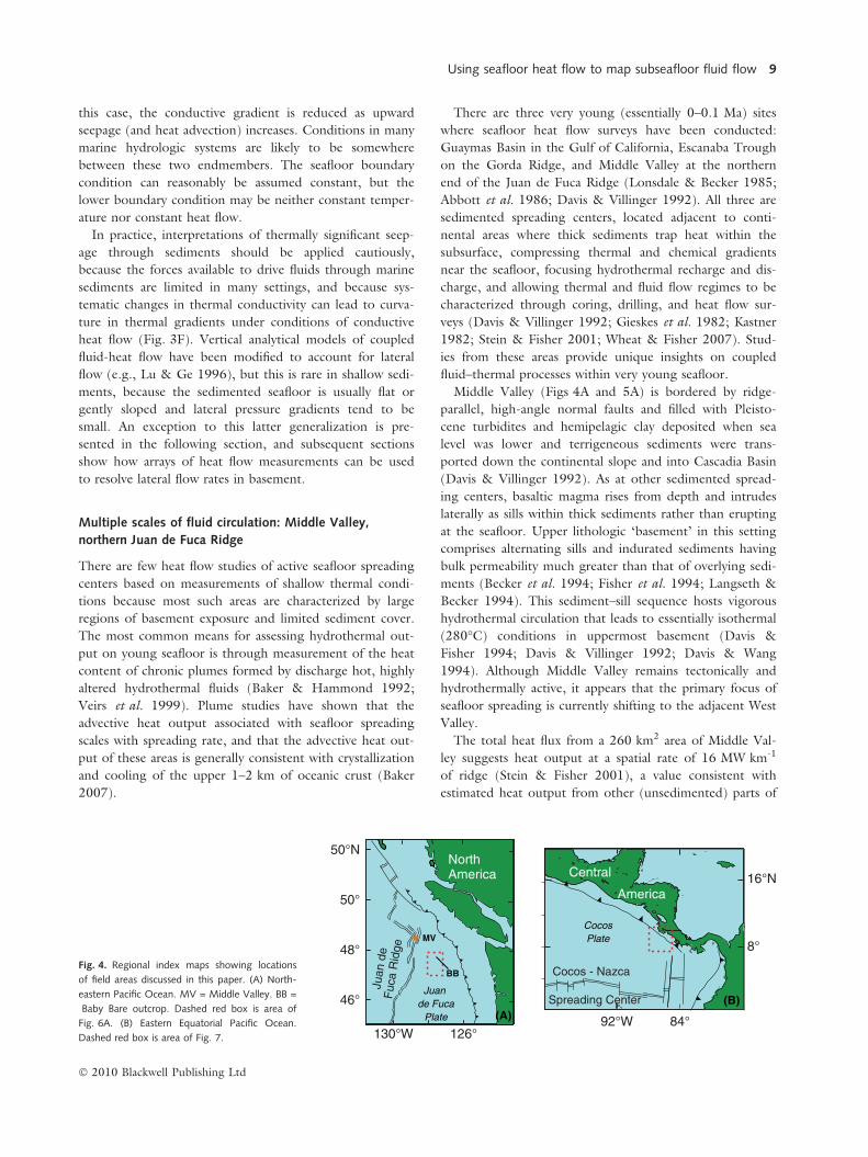
BBFig. 4. Regional index maps showing locations

of field areas discussed in this paper. (A) North-

eastern Pacific Ocean. MV = Middle Valley. BB =

Baby Bare outcrop. Dashed red box is area of

Fig. 6A. (B) Eastern Equatorial Pacific Ocean.

Dashed red box is area of Fig. 7.

Using seafloor heat flow to map subseafloor fluid flow 9

� 2010 Blackwell Publishing Ltd

the Juan de Fuca Ridge (Baker 2007). But in contrast to

more normal seafloor spreading centers, conductive and

advective heat outputs from Middle Valley are about equal

in magnitude. Bare rock spreading centers are thought to

release the vast majority of their heat advectively.

The Dead Dog vent field within Middle Valley has been

explored with numerous instruments, including a side-scan

survey that defined the area of active venting (AAV) based

on high acoustic backscatter (Davis & Villinger 1992)

(Fig. 5B). Within the AAV there are �20 vents discharging

hydrothermal fluid at temperatures up to 280�C. A scien-

tific drill hole placed near the center of this AAV cored

extrusive basaltic rocks below �260 of turbidites and

hemipelagic clay. Repeated heat flow surveys (including

data from multipenetration probes and outriggers probes

attached to core barrels) show that the highest values are

found immediately adjacent to active vents (Fig. 5B).

Interestingly, some of the lowest heat flow values were also

measured close to active vents.

The mean heat flow of �10 W m–2 within the Dead

Dog AAV has been interpreted to result from formation of

a diagenetic and hydrologic cap above a shallow hydrother-

mal reservoir (Davis & Villinger 1992; Davis & Fisher

1994; Stein et al. 1998; Stein & Fisher 2001). Fluid con-

vects vigorously below the cap, helping to maintain iso-

thermal conditions near 280�C at �30 m below the

seafloor. There may be additional focusing of conductive

heat flow because of refraction related to the buried base-

ment edifice and shallow sulfide deposits, both of which

have greater thermal conductivity than typical marine sedi-

ments (Fig. 3A).

The scattering of heat flow values both above and below

the mean of �10 W m-2 within the AAV can be explained

by proximity to active vents, as demonstrated with coupled

numerical modeling (Fig. 5C and D). The vents act as

conductive heat sources as hydrothermal fluid rises to the

seafloor, warming shallow sediments around the vents, and

elevating heat flow to values ‡50 W m-2. In addition, local

recharge associated with secondary convection can suppress

heat flow to <1 W m-2 close to vents. This secondary con-

vection cannot be a significant mechanism for recharging

the main hydrothermal system because fluid samples col-

lected from the vents show no indication of mixing

between hydrothermal fluid and ambient seawater, and

there is little evidence for water–sediment interaction prior

to fluid discharge (Butterfield et al. 1994). Instead, it is

likely that recharge of fluids supporting high-temperature

discharge in Middle Valley occurs mainly along faults and

128o42.8'W 42.6' 42.4'

q (W m–2)<22-44-10>10

(B)

T = 2 oC, Free flow

T =

280

oC

T = 280 oC, No flow

No

flow

A

B

0

10

20

10 20 30 40

Heat flow

(W/m

2)

Distance from vent (m)

No connection to vent

B-13

A-12B-12

A-13

Mean vent field heat flow

Minimum vent field heat flow

(C)

(D)

48o 27.2'

2N

7.6'27.4'

128o 50' W 40'

>1 W m–2

0.2

0.40.6

0.4

0.4

0.6

0.8

0.8 0.4

0.6 0.

4

0.6

0.6

48o

20'

3N

0'

200 m100010 km50

active vent

(A)

Fig. 5. Diagrams showing data and model results from Middle Valley, northern Juan de Fuca Ridge. Figures modified from Davis & Villinger (1992) and Stein

& Fisher (2001). (A) Regional view of Middle Valley, showing valley bounding normal faults (thin lines with ticks) and area of the most complete coverage of

seafloor heat flow measurements (within thicker dashed line). Contours show typical heat flow values (units of W m-2), and grey areas show where heat flow

is ‡1 W m-2. Dotted box shows area of Fig. 5B. (B) Area of active venting (AAV) including the Dead Dog vent field. Edge of AAV identified by side scan

sonar surveys (Davis & Villinger 1992). Open circles indicate location and magnitude of heat flow values, as labeled. Solid squares are individual hydrothermal

vents. Crosses indicate at least one thermistor exceeded maximum temperature range of instrument (40�C). Stars indicate locations where the heat flow

probe fell over without penetrating. (C) Schematic of radial cross-section used in simulations of secondary circulation around a hydrothermal vent. Horizontal

(10 and 20 mbsf) and vertical (20 m from vent) 1-m thick channels were used in some simulations, labeled to show flow paths A and B, respectively.

(D) Surface heat flow versus distance from vent for simulations with secondary hydrothermal convection. Background heat flow is 10 W m-2. Conductive

case is shown for reference with no connection to vent. Cases A and B have a shallower and deeper connection to the hydrothermal vent, respectively, and

each is run with connection permeability of 10-12 m2 and 10-13 m2 as shown. The deeper the horizontal layer and the higher its permeability, the more effi-

cient the local heat flow reduction associated with secondary convection.

10 A. T. FISHER & R. N. HARRIS

� 2010 Blackwell Publishing Ltd

other isolated conduits along the edges of the valley (Davis

& Villinger 1992; Stein & Fisher 2001; Wheat & Fisher

2007). In summary, heat flow and other data from Middle

Valley resolve multiple scales of fluid circulation, delineate

conditions and the depth to the top of a hydrothermal res-

ervoir, and help to define the regional geometry of fluid

flow, including the importance of basement outcrops in

guiding hydrothermal recharge. The extent to which these

results can be applied to more normal (bare rock) seafloor

spreading centers remains to be determined.

FLUID FLOW THROUGH OUTCROPS:EASTERN FLANK OF THE JUAN DE FUCARIDGE

Numerous physical and chemical surveys have been com-

pleted on 0.7–3.6 Ma seafloor on the eastern flank of the

Juan de Fuca Ridge (Davis et al. 1992, 1999; Wheat &

Mottl 1994, 2000; Thomson et al. 1995; Elderfield et al.

1999; Fisher et al. 2003a; Hutnak et al. 2006; Wheat et al.

2004). Oceanic basement rocks in this area were formed at

the unsedimented Endeavour segment of the Juan de Fuca

Ridge, but were subsequently covered at a young age by

hemipelagic clay and turbidites. Basement rocks remain

exposed close to the active spreading center and where sea-

mounts and other basement outcrops are found up to

100 km to the east. Three basement outcrops were identi-

fied initially in this area: Papa Bare, Mama Bare, and Baby

Bare (Fig. 6A) (Davis et al. 1992; Thomson et al. 1995;

Mottl et al. 1998). These outcrops are volcanic cones cre-

ated off-axis on top of preexisting abyssal hill topography.

Baby Bare outcrop is the smallest and most extensively

surveyed of the three outcrops, rising 70 m above the sur-

rounding seafloor and covering an area of 0.5 km2.

Although the elevated area of this feature is small, the bur-

ied Baby Bare edifice rises �600 m above the top of regio-

nal volcanic crustal rocks. Analysis of altered rocks,

sediment pore fluids, and shallow thermal gradients on

Baby Bare outcrop indicate that this feature discharges

5–20 L s-1 of hydrothermal fluid (Thomson et al. 1995;

Mottl et al. 1998; Becker et al. 2000; Wheat et al. 2004).

Mama and Papa Bare outcrops (Fig. 6A) are also sites of

ridge-flank hydrothermal discharge, although these features

have not been surveyed as completely as Baby Bare. Mama

Bare outcrop is located 14 km northeast of Baby Bare out-

crop on the same basement ridge, covers an area of

0.9 km2, and rises 140 m above the surrounding seafloor.

Papa Bare outcrop is located on an adjacent buried

(A) (B)

Fig. 6. Maps of field area on the eastern flank of the Juan de Fuca Ridge (index map shown in Fig. 4A). (A) Regional map showing locations of basement

outcrops on 3.5–3.6 Ma seafloor (modified from Hutnak et al. 2006). Baby Bare, Mama Bare, and Papa Bare outcrops are sites of hydrothermal discharge,

whereas Grizzly Bare is a site of hydrothermal recharge (Fisher et al. 2003a). (B) Fine scale topographic map of Baby Bare outcrop, with locations of heat

flow measurements made with the submersible, Alvin (Wheat et al. 2004). Highest heat flow values are associated with a normal fault on the eastern side of

the outcrop. Several of these heat flow values are based on curved gradients, as shown in the inset diagram. Numbers in the inset indicate apparent seepage

rates, in m year-1, based on application of the model shown in Fig. 3D.

Using seafloor heat flow to map subseafloor fluid flow 11

� 2010 Blackwell Publishing Ltd

basement ridge to the east, covers an area of 2.6 km2, and

rises 240 m above the surrounding seafloor. As with Baby

Bare outcrop, most of the Papa and Mama Bare edifices

are buried by thick sediments. Interestingly, no hydrother-

mal recharge sites have been identified on any of these

three features.

Consideration of ridge-flank hydrothermal driving

forces, basement fluid chemistry, and sediment properties

precludes recharge of Baby Bare outcrop through the sea-

floor surrounding the basement edifice; instead, fluids

recharge through Grizzly Bare outcrop 52 km to the south

(Fig. 6A) (Fisher et al. 2003a). Grizzly Bare outcrop is

conical in shape, 3.5 km in diameter, and rises 450 m

above the surrounding seafloor. The consistency of their

alignment and strike with regional basement topography

(Wilson 1993; Zuhlsdorff et al. 2005) suggests that the

Grizzly, Baby, and Mama Bare outcrops may have formed

along the same buried abyssal hill. Fluid flow in basement

between Grizzly Bare and Baby Bare outcrops may be facil-

itated by enhanced permeability in a direction parallel to

the abyssal hill topography (Fisher et al. 2003a, 2008;

Wheat et al. 2000). Grizzly Bare outcrop was identified as

a site of hydrothermal recharge based initially on patterns

of seafloor heat flow immediately adjacent to the edifice.

Seafloor heat flow is depressed within a few kilometers of

the edge of basement exposure along several transects of

measurements (Fisher et al. 2003a; Hutnak et al. 2006).

Seismic reflection data allow determination of sediment

thicknesses at heat flow measurement locations, and down-

ward continuation of thermal data through the sediment

shows that isotherms are swept downwards by cold,

recharging fluid in the sediments and shallow basement

adjacent to the outcrop edge. In contrast, warm fluid dis-

charge from Baby Bare outcrop causes extremely high sea-

floor heat flow, and an upward sweeping of isotherms,

adjacent to the area of exposed basement (Davis et al.

1992; Fisher et al. 2003a).

Baby Bare outcrop was surveyed repeatedly using the

submersible Alvin, including high-resolution bathymetric

mapping, geological and pore fluid sampling, and heat flow

measurements (Wheat et al. 2004) (Fig. 6B). The Alvin

heat flow probes used on these surveys were �0.60 m long

and contained three or five thermistors. A constant thermal

conductivity of 0.89 W (m �C)-1 was assumed for all Baby

Bare heat flow measurements (Wheat et al. 2004), based

on in situ and needle probe measurements of material

recovered nearby during subsequent surveys (Fisher et al.

2003a; Hutnak et al. 2006). Most heat flow values mea-

sured on Baby Bare outcrop were >1 W m-2, well above

values measured on the adjacent flat seafloor, and the high-

est Baby Bare values were >100 W m-2. There is an area of

elevated heat flow aligned along a linear trend on the

southwest side of the outcrop, adjacent to a normal fault

scarp near the outcrop summit (Fig. 6B). Sediment thick-

ness is not well mapped across Baby Bare outcrop because

of irregular topography, but the depth to the 64�C iso-

therm (consistent with regional basement temperatures

and fluid chemistry) is generally £50 m (Davis et al. 1992;

Elderfield et al. 1999; Hutnak et al. 2006; Wheat & Fisher

2007).

Several thermal profiles from Baby Bare outcrop display

significant curvature with depth. These thermal profiles

were interpreted to indicate fluid flow, through applica-

tion of the Bredehoeft & Papadopulos (1965) model

(Fig. 3D), only if curvature could not be accounted for

by reasonable variations in thermal conductivity, and only

if the apparent seepage rate exceeded 6.5 m year-1

(Fig. 6B, inset, Wheat et al. 2004). Other profiles, indi-

cating apparently conductive thermal conditions, were

evaluated based on nearby geochemical data from push

cores. Geochemical data were fit to an advection–diffusion

model similar to that used for assessing curvature in ther-

mal data. But because chemical diffusivity for solutes is

about three orders of magnitude smaller than thermal dif-

fusivity, chemical data are much more sensitive to fluid

flow. Chemical data were used to estimate seepage rates

between 0.005 and 2 m year-1, above which chemical

concentrations are essentially constant with depth in the

upper 0.5 m of sediment. Total heat flow values were cal-

culated as the sum of conductive and advective compo-

nents (Wheat et al. 2004).

Thermal and chemical data were combined to estimate

point and total seepage rates, and integrated heat output,

from Baby Bare outcrop. These data suggest heat output

of �2 MW for Baby Bare and the immediately surrounding

seafloor, a value similar to that estimated in earlier seafloor

studies (Mottl et al. 1998), and at the lower end of esti-

mates made from thermal anomalies in the overlying water

column (Thomson et al. 1995). Estimated Baby Bare heat

output is about the same as that from a single high-tem-

perature (350�C) hydrothermal vent. The mean heat flow

from Baby Bare outcrop is an order of magnitude greater

than that estimated from lithospheric cooling models for

3.5 Ma seafloor like that upon which Baby Bare is located.

Although there are small areas on Baby Bare outcrop

where shimmering water can be seen rising from the sea-

floor, the thin drape of sediment overlying much of the

basement edifice functions effectively as a thermal bound-

ary layer, with vigorous convection in the underlying base-

ment redistributing heat laterally and enhancing the rate of

conduction through the top of the edifice. Advective heat

loss from Baby Bare outcrop is limited, and the present

day circulation system has virtually no influence on regio-

nal heat flow (Davis et al. 1999; Hutnak et al. 2006),

although it is likely that advective heat loss was consider-

ably greater in the past, before many other outcrops were

covered by thick, low-permeability sediments (Hutnak &

Fisher 2007).

12 A. T. FISHER & R. N. HARRIS

� 2010 Blackwell Publishing Ltd

Massive fluid fluxes resolved with thermal data: Eastern

Cocos Plate

The 18–24 Ma seafloor of the Cocos Plate offshore the

Nicoya Peninsula, Costa Rica (Fig. 4B), comprises a northern

region formed at the East Pacific Rise (EPR), and a south-

ern region formed at the Cocos-Nazca Spreading Center

(CNS) (Fig. 7) (Meschede et al. 1998; Ranero & von

Huene 2000; von Huene et al. 2000; Barckhausen et al.

2001). The boundary between EPR- and CNS-generated

seafloor is a combination of a triple junction trace and a

fracture zone trace, collectively comprising a ‘plate suture.’

Pre-2000 studies in this area revealed variable thermal con-

ditions (e.g., Langseth & Silver 1996; Vacquier et al.

1967; Von Herzen & Uyeda 1963), but the spatial distri-

bution of warmer and cooler seafloor was incomplete, and

the extent and nature of hydrothermal activity was unclear.

Later surveys included swath-mapping to identify basement

outcrops, and multi-channel seismic reflection data to

delineate regional tectonic features, sediment thickness,

and basement relief (Fisher et al. 2003b; Hutnak et al.

2007). Multipenetration heat flow data were co-located on

seismic reflection profiles to assess heat transport and

determine upper basement temperatures; additional heat

flow measurements were made with autonomous tempera-

ture probes attached to core barrels (Pfender & Villinger

2002; Hutnak et al. 2007).

Heat flow surveys documented a thermal transition

between warm and cool areas of the Cocos Plate (Fisher

et al. 2003b; Hutnak et al. 2007) (Fig. 7). The mean heat

flow through CNS- and EPR-generated seafloor on the

warm part of the plate is consistent with lithospheric ther-

mal reference models, 95–120 mW m-2 (Parsons & Sclater

1977; Stein & Stein 1994). In contrast, the seafloor heat

flow through EPR-generated seafloor northwest of the

thermal transition is typically 10–40 mW m-2, just 10–40%

of lithospheric values. The thermal transition between

warm and cool areas of the plate is only a few kilometers

wide (Fig. 8), consistent with advective heat extraction

from the shallow crust on the cool side of the plate (Fisher

et al. 2003b; Hutnak et al. 2007). The thermal transition

coincides with the plate suture near where the Cocos Plate

begins to subduct in the Middle America Trench. But

through most of the survey area, the boundary between

warmer and cooler parts of the plate is spatially associated

with the occurrence of seamounts and other basement out-

crops that penetrate regionally extensive sediments

(Fig. 7).

(A) (B)

Fig. 7. A. Bathymetric map of field area on 18–24 Ma seafloor of the Cocos Plate, eastern Pacific Ocean (index map shown in Fig. 4B) (modified from Hut-

nak et al. 2008). Dorado outcrop is a site of hydrothermal discharge, whereas Tengosed Seamount is a site of hydrothermal recharge. Gray line demarcates

thermal boundary between cooler and warmer parts of the plate. (B) Major tectonic features and results of heat flow surveys. Gray area is cool part of Cocos

Plate. Black circles and ovals are seamounts and other basement outcrops apparent on satellite and swath data. EPR = East Pacific Rise. CNS = Cocos-Nazca

Spreading Center.

Using seafloor heat flow to map subseafloor fluid flow 13

� 2010 Blackwell Publishing Ltd

Heat flow and seismic surveys oriented radially away

from outcrops indicate that some allow hydrothermal

recharge whereas others allow hydrothermal discharge

(Hutnak et al. 2007, 2008), a pattern similar to that seen

on younger seafloor east of the Juan de Fuca Ridge (Davis

et al. 1992; Fisher et al. 2003a; Hutnak et al. 2006). Seis-

mic and heat flow data across Tengosed Seamount and

Dorado ourcrop, areas of basement exposure separated by

20 km, illustrate characteristic features of this circulation

pattern (Figs 7 and 9). Cold fluid recharge is indicated by

14 00012 00010 00080006000

Hea

t flo

w (

mW

m–2

)

20

60

100

CDP

NW SE

Heat loss dominantly conductive

Heat loss dominantly advective

Conductive lithospheric cooling

4000

4400

4800

5200Two-

way

trav

el ti

me

(ms)

10°C

20°C30°C 50°C

Seafloor

Sediments

Basement

4 8 12 km0

Fig. 8. Co-located heat flow and seismic data that cross the thermal transition between cool and warm parts of the Cocos Plate (location shown in Fig. 7A).

Horizontal axis is common depth point (CDP) of the seismic survey. Diagonal band shows range of lithospheric values predicted by standard models for sea-

floor of this age. Transition between cool and warm parts of the plate occurs across �2 km, indicating an abrupt change in mechanisms of heat transport in

the shallow crust, with vigorous hydrothermal cooling on the northwest side of the transition, and conductive (lithospheric) conditions on the southeast side

(Fisher et al. 2003b). Isotherms superimposed on the seismic section were calculated by downward continuing heat flow measurements (Hutnak et al. 2007).

(A) (B)

Fig. 9. (A) Seismic and heat flow data near and across Dorado outcrop (location shown in Fig. 7A). Basement rises to penetrate 400–500 m of regionally

continuous sediment, and is exposed across a small area of seafloor. Isotherms (black lines) created by downward continuation of heat flow data. Heat flow

rises abruptly near the edge of the edifice, but basement temperatures are nearly isothermal at 10–20�C beyond several kilometers from the outcrop.

(B) Seismic and heat flow data adjacent to Tengosed Seamount, 20 km east of Dorado (location shown in Fig. 7A). Note differences in vertical scale relative

to panel A. Tengosed Seamount is a large edifice rising >1 km above the seafloor, 2 km above regional basement. The upper crust here is chilled below thick

sediments by cold bottom water that recharges through exposed basement. Heat flow (and basement temperatures) rise �10 km south of the outcrop, after

passing through the regional thermal transition (dashed red line).

14 A. T. FISHER & R. N. HARRIS

� 2010 Blackwell Publishing Ltd

a decrease in seafloor heat flow and a downward sweeping

of isotherms where sediment thins in proximity to an out-

crop. In contrast, warm fluid discharge results in locally

elevated seafloor heat flow, and an upward sweeping of iso-

therms adjacent to an area of exposed basement. In the lat-

ter case, the temperature of the sediment–basement

contact often remains nearly isothermal as the contact shal-

lows towards the seafloor.

Regional advective power and fluid fluxes from the cold

part of the Cocos Plate were quantified using the conduc-

tive heat flow deficit (Hutnak et al. 2008). There is a

14,500 km2 area of cool lithosphere on the EPR side of

the Cocos Plate. The mean heat flow in this area, away

from the local conductive influence basement outcrops and

buried ridges, is 29 ± 13 mW m-2 (±1 SD), comprising a

regional power deficit of 0.8–1.4 GW. Heat flow profiles

adjacent to five of the ten mapped basement outcrops in

this area indicate recharge through two, discharge through

one (Dorado outcrop), one that both recharges and dis-

charges, and one that shows evidence for neither recharge

nor discharge (Hutnak et al. 2008).

The mean advective power output of individual discharg-

ing outcrops on cooler TicoFlux seafloor is 200–350 MW,

a range similar to that determined from plume and point

studies of high-temperature vent fields on the southern

Cleft segment of the Juan de Fuca Ridge (JdFR) and 21�Non the EPR (at the low end) and the Endeavour Main

Field on the JdFR and 9�50’N on the EPR (at the high

end) (Baker 2007). But in contrast to these ridge-crest sys-

tems, the enormous advection of heat from a few outcrops

on the Cocos Plate is conveyed by fluids having tempera-

tures only 5–40�C warmer than bottom water (Hutnak

et al. 2008). Thermal data from the cool side of the Cocos

Plate indicate 4–80 · 103 L s-1 of fluid enters and exits the

seafloor in this area. If this fluid flow were distributed

across the discharging outcrops, consistent with interpreta-

tions from the heat flow surveys, then each discharging

outcrop vents 1–20 · 103 L s-1 of cool hydrothermal fluid

(Hutnak et al. 2008).

SUMMARY, LESSONS LEARNED, ANDPROSPECTS FOR FUTURE WORK

Marine heat flow measurements have helped to quantify

fluid flow patterns and rates within the seafloor for more

than 30 years. Even before the discovery of seafloor hydro-

thermal vents, researchers used variations in oceanic heat

flow to quantify the extent and nature of hydrogeologic

processes in the deep sea. Heat flow data are most useful

for this purpose when they are carefully navigated and co-

located with reflection seismic and mapping data, so that

thermal measurements can be placed in a broader context.

It is also helpful to combine thermal studies with coring

and chemical analyses, and to obtain high-resolution

images or direct observations of seafloor conditions, so

that the significance of small-scale variations in heat output

can be understood. This has become the standard mode of

operation for modern seafloor heat flow studies.

Although the studies described in this review were com-

pleted in different hydrogeologic settings, they share sev-

eral common themes. Marine sediments generally function

as a conductive boundary layer separating the volcanic

crustal aquifer from the overlying ocean. This is a benefit

for using seafloor heat flow to map fluid flow, because the

(sedimentary) conductive boundary layer provides a rela-

tively continuous medium in which measurements can be

made, and across which thermal conditions can be deter-

mined. There may be thermally significant fluid flow

through marine sediments in some locations, but demon-

strating this requires that curvature in thermal gradients

cannot be explained by reasonable differences in thermal

conductivity.

In fact, thermally significant fluid seepage through sea-

floor sediments is relatively rare, being restricted to locations

where sediments are thin or unusually permeable, or where

driving forces are unusually high. Patterns of conductive

heat flow through marine sediments can be used to map out

directions and assess rates of fluid circulation within the

underlying crust, and are particularly helpful in identifying

locations of fluid recharge and discharge near where base-

ment rocks are exposed. Seafloor heat flow measurements

are less helpful in resolving the nature of fluid pathways at

depth within the crust, but this issue is being addressed to

some extent with analysis of core samples and single-hole

and multi-hole measurements and experiments (e.g., Becker

et al. 1983; Anderson et al. 1985; Bartetzko et al. 2001; Alt

& Teagle 2003; Becker & Davis 2005; Fisher et al. 2008).

The continued interest in using heat as a tracer to map

fluid flow; more common acquisition of complementary

data such as high-resolution digital maps and seismic

reflection profiles; and the development of new instru-

ments, analytical techniques, and models, is bringing new

attention and new practitioners to the field. Most of the

seafloor remains poorly mapped and virtually unexplored

with regard to thermal and hydrogeologic conditions. Sea-

floor heat flow remains an important tool for researchers

studying coupled fluid, thermal, chemical, tectonic, mag-

matic, and biological processes. Heat flow measurements

are particularly helpful for quantifying local and regional

heat and fluid flow rates, and for mapping the plumbing of

subseafloor hydrogeologic systems.

ACKNOWLEDGMENTS

This work was supported by National Science Foundation

grants OCE-0727952 and OCE-0849354 (ATF) and

grants OCE-0637120 and OCE-0849341 (RNH).

The authors appreciate thoughtful comments by two

Using seafloor heat flow to map subseafloor fluid flow 15

� 2010 Blackwell Publishing Ltd

external reviewers that improved the clarity and focus of

this paper.

REFERENCES

Abbott DH, Morton JL, Holmes ML (1986) Heat flow measure-

ments on a hydrothermally active, slow spreading ridge: theEscanaba Trough. Geophysical Research Letters, 13, 678–80.

Alt JC, Teagle DAH (2003) Hydrothermal alteration of upper

oceanic crust formed at a fast spreading ridge: mineral, chemical,and isotopic evidence from ODP Site 801. Chemical Geology,201, 191–211.

Anderson MP (2005) Heat as a ground water tracer. GroundWater, 43, 1–18.

Anderson RN, Hobart MA (1976) The relationship between heat

flow, sediment thickness, and age in the eastern Pacific. Journalof Geophysical Research, 81, 2968–89.

Anderson RN, Zoback MD, Hickman SH, Newmark RL (1985)Permeability versus depth in the upper oceanic crust: in-situ

measurements in DSDP Hole 504B, eastern equatorial Pacific.

Journal of Geophysical Research, 90, 3659–69.Baker ET (2007) Hydrothermal cooling of midocean ridge axes:

Do measured and modeled heat fluxes agree. Earth and Plane-tary Science Letters, 263, 140–50.

Baker ET, Hammond SR (1992) Hydrothermal venting and theapparent magmatic budget of the juan de fuca ridge. Journal ofGeophysical Research, 97, 3443–56.

Baker ET, Massoth GJ, Feely RA, Embly RW, Thomson RE, Burd

BJ (1995) Hydrothermal event plumes from the CoAxial sea-floor eruption site, Juan de Fuca Ridge. Geophysical ResearchLetters, 22, 147–50.

Barckhausen U, Renaro C, von Huene R, Cande SC, Roeser HA(2001) Revised tectonic boundaries in the Cocos Plate off Costa

Rica: implications for the segmentation of the convergent mar-

gin and for plate tectonic models. Journal of GeophysicalResearch, 106, 19.

Barker P, Lawver L (2000) Anomalous temperatures in central

Scotia Sea sediments – bottom water variation or pore water

circulation in old crust. Geophysical Research Letters, 27, 13–6.

Bartetzko A, Pezard P, Goldberg D, Sun Y-F, Becker K (2001)Volcanic stratigraphy of DSDP ⁄ ODP Hole 395A: an interpreta-

tion using well-logging data. Marine Geophysical Researches, 22,

111–27.

Becker K, Davis EE (2005) A review of CORK designs and opera-tions during the Ocean Drilling Program. In: Proc. IODP, Expe-dition Reports (eds Fisher AT, Urabe T, Klaus A) College

Station, TX, Integrated Ocean Drilling Program, 301,doi:10.2204/iodp.proc.2301.2104.

Becker K, Langseth M, Von Herzen RP, Anderson R (1983) Deep

crustal geothermal measurements, Hole 504B, Costa Rica Rift.

Journal of Geophysical Research, 88, 3447–57.Becker K, Morin RH, Davis EE (1994) Permeabilities in the Mid-

dle Valley hydrothermal system measured with packer and flow-

meter experiments. In: Proc. ODP, Sci. Res. (eds Davis EE,

Mottl MJ, Fisher AT, Slack JF) College Station, TX, OceanDrilling Program, 139, 613–26.

Becker NC, Wheat CG, Mottl MJ, Karsten JL, Davis EE (2000) A

geological and geophysical investigation of Baby Bare, locus of aridge flank hydrothermal system in the Cascadia Basin. Journalof Geophysical Research, 105, 23, 557–568.

Bredehoeft JD, Papadopulos IS (1965) Rates of vertical ground-

water movement estimated from the earth’s thermal profile.Water Resources Research, 1, 325–8.

Bullard EC (1939) Heat flow in South Africa. Proceedings of theRoyal Society of London, Series A., 173, 474–502.

Bullard EC (1954) The flow of heat through the floor of the

Atlantic Ocean. Proceedings of the Royal Society of London, SeriesA, 222, 408–29.

Bullard EC, Maxwell AE (1956) Heat flow through the deep sea

floor. Advances in Geophysics, 222, 408–29.

Burow KR, Constantz J, Fujii R (2005) Heat as a tracer to esti-mate dissolved organic carbon flux from a restored wetland.

Ground Water, 43, 545–56.

Butterfield DA, McDuff RE, Franklin J, Wheat CG (1994) Geo-

chemistry of hydrothermal vent fluids from Middle Valley, Juande Fuca Ridge. In: Proc. ODP, Sci. Res. (eds Davis EE, Mottl

MJ, Fisher AT, Slack JF) College Station, TX, Ocean DrillingProgram, 139, 395–410.

Constantz J, Stonestrom D, Stewart AE, Niswonger R, Smith TR(2001) Analysis of streambed temperatures in ephemeral chan-

nels to determine streamflow frequency and duration. WaterResources Research, 37, 317–28.

Davis EE (1988) Oceanic heat-flow density. In: Handbook of Ter-restrial Heat-Flow Density Determination (eds Haenel R, Rybach

L, Stegena L), pp. 223–60. Kluwer, Amsterdam.

Davis EE, Becker K (1994) Formation temperatures and pressuresin a sedimented rift hydrothermal system: 10 months of CORK

observations, Holes 857D and 858G. In: Proc. ODP, Sci. Res.(eds Davis EE, Mottl MJ, Fisher AT, Slack JF) College Station,

TX, Ocean Drilling Program, 139, 649–66.Davis EE, Becker K (2002) Observations of natural-state fluid

pressures and temperatures in young oceanic crust and infer-

ences regarding hydrothermal circulation. Earth and PlanetaryScience Letters, 204, 231–48.

Davis EE, Fisher AT (1994) On the nature and consequences of

hydrothermal circulation in the Middle Valley sedimented rift:

inferences from geophysical and geochemical observations, Leg139. In: Proc. ODP, Sci. Res. (eds Davis EE, Mottl MJ, Fisher

AT, Slack JF) College Station, TX, Ocean Drilling Program,

139, 695–717.

Davis EE, Lister CRB (1974) Fundamentals of ridge crest topog-raphy. Earth and Planetary Science Letters, 21, 405–13.

Davis EE, Villinger H (1992) Tectonic and thermal structure of

the Middle Valley sedimented rift, northern Juan de Fuca Ridge.

In: Proc. ODP, Init. Repts. (eds Davis EE, Mottl M, Fisher AT)College Station, TX, Ocean Drilling Program, 139, 9–41.

Davis EE, Wang K (1994) Present and past temperatures of sedi-

ments at Site 857, Middle Valley, northern Juan de Fuca Ridge.In: Proc. ODP, Sci. Res. (eds Davis EE, Mottl MJ, Fisher AT, Slack

JF) College Station, TX, Ocean Drilling Program, 139, 565–72.

Davis EE, Chapman DS, Forster C, Villinger H (1989) Heat-flow

variations correlated with buried basement topography on theJuan de Fuca Ridge flank. Nature, 342, 533–7.

Davis EE, Chapman DS, Mottl MJ, Bentkowski WJ, Dadey K,

Forster C, Harris R, Nagihara S, Rohr K, Wheat G, Whiticar M

(1992) FlankFlux: an experiment to study the nature of hydro-thermal circulation in young oceanic crust. Canadian Journal ofEarth Sciences, 29, 925–52.

Davis EE, Villinger H, Macdonald RD, Meldrum RD, Grigel J(1997a) A robust rapid-response probe for measuring bottom-

hole temperatures in deep-ocean boreholes. Marine GeophysicalResearches, 19, 267–81.

Davis EE, Wang K, He J, Chapman DS, Villinger H, RosenbergerA (1997b) An unequivocal case for high Nusselt-number hydro-

thermal convection in sediment-buried igneous oceanic crust.

Earth and Planetary Science Letters, 146, 137–50.

16 A. T. FISHER & R. N. HARRIS

� 2010 Blackwell Publishing Ltd

Davis EE, Chapman DS, Wang K, Villinger H, Fisher AT, Robin-son SW, Grigel J, Pribnow D, Stein J, Becker K (1999) Regio-

nal heat-flow variations across the sedimented Juan de Fuca

Ridge eastern flank: constraints on lithospheric cooling and lat-

eral hydrothermal heat transport. Journal of GeophysicalResearch, 104, 17, 675–88.

Davis EE, Wang K, Becker K, Thomson RE, Yashayaev I (2003)

Deep-ocean temperature variations and implications for errors inseafloor heat flow determinations. Journal of GeophysicalResearch, 108, 2034. doi:2110.1029/2001JB001695.

Elder JW (1965) Physical processes in geothermal areas. In: Terres-trial Heat Flow (ed Lee WHK) Washington, DC, AmericanGeophysics Union, 8, 211–39.

Elderfield H, Wheat CG, Mottl MJ, Monnin C, Spiro B (1999)

Fluid and geochemical transport through oceanic crust: a tran-

sect across the eastern flank of the Juan de Fuca Ridge. Earthand Planetary Science Letters, 172, 151–65.

Fisher AT, Becker K (1993) A guide for ODP tools for downhole

measurements, Technical note 10, doi: 10.2973/odp.tn.10.1993. Available at: http://www-odp.tamu.edu/publications/

tnotes/tn10/10toc.html (accessed 31 December 2009).

Fisher AT, Becker K (2000) Channelized fluid flow in oceanic

crust reconciles heat-flow and permeability data. Nature, 403,71–4.

Fisher AT, Becker K, Narasimhan TN, Langseth MG, Mottl MJ

(1990) Passive, off-axis convection on the southern flank of the

Costa Rica Rift. Journal of Geophysical Research, 95, 9343–70.Fisher AT, Fischer K, Lavoie D, Langseth M, Xu J (1994) Hydro-

geological and geotechnical properties of shallow sediments at

Middle Valley, northern Juan de Fuca Ridge. In: Proc. ODP,Sci. Res. (eds Mottl MJ, Davis EE, Fisher AT, Slack JF) College

Station, TX, Ocean Drilling Program, 139, 627–48.

Fisher AT, Becker K, Davis EE (1997) The permeability of young

oceanic crust east of Juan de Fuca Ridge determined using bore-hole thermal measurements. Geophysical Research Letters, 24,

1311–4.

Fisher AT, Davis EE, Hutnak M, Spiess V, Zuhlsdorff L, Cherka-

oui A, Christiansen L, Edwards KM, Macdonald R, Villinger H,Mottl MJ, Wheat CG, Becker K (2003a) Hydrothermal

recharge and discharge across 50 km guided by seamounts on a

young ridge flank. Nature, 421, 618–21.

Fisher AT, Stein CA, Harris RN, Wang K, Silver EA, Pfender M,Hutnak M, Cherkaoui A, Bodzin R, Villinger H (2003b)

Abrupt thermal transition reveals hydrothermal boundary and

role of seamounts within the Cocos Plate. Geophysical ResearchLetters, 30, 1550, doi:1510.1029/2002GL016766.

Fisher AT, Villinger H, Heesemann M (2007) User Manual forthe Third-Generation, Advanced Piston Corer Temperature tool(APCT-3). Integrated Ocean Drilling Program, College Station,TX.

Fisher AT, Davis EE, Becker K (2008) Borehole-to-borehole

hydrologic response across 2.4 km in the upper oceanic crust:

implications for crustal-scale properties. Journal of GeophysicalResearch, 113, B07106, doi:10.1029/2007JB005447.

Foucher J-P, Henry P, Harmegnies F (1997) Long-term observa-

tions of pressure and temperature in Hole 948D, Barbadosaccretionary prism. In: Proc. ODP, Sci. Res. (eds Ogawa Y, Ship-

ley T, Blum P, Bahr J) College Station, TX, Ocean Drilling Pro-gram, 156, 239–46.

Fukasawa M, Freeland H, Perkin R, Wantanabe T, Uchida H,Nishina A (2003) Bottom water warming in the North Pacific

Ocean. Nature, 427, 825–7.

Gieskes J, Kastner M, Einsele G, Kelts K, Niemitz J (1982)

Hydrothermal activity in the Guayman Basin, Gulf of California,

a synthesis. In: Init. Repts., DSDP (eds Curray J, Moore D),U. S. Govt. Printing Office, Washington, D. C., 64, 1159–68.

Goto S, Yamano M, Kinoshita H (2005) Thermal response of sed-

iment with vertical fluid flow to periodic temperature variation

at the surface. Journal of Geophysical Research, 110, B01106,doi:10.1029/2004JB003419.

Hamamoto H, Yamano M, Goto S (2005) Heat flow measure-

ment in shallow seas through long-term temperature monitor-ing. Geophysical Research Letters, 32, L21311.

Harris RN, Chapman DS (2004) Deep-seated oceanic heat flow,

heat deficits, and hydrothermal circulation. In: Hydrogeology ofthe Oceanic Lithosphere (eds Davis EE, Elderfield H), pp. 311–36. Cambridge University Press, Cambridge, UK.

Harris RN, Von Herzen RP, McNutt MK, Garven G, Jordahl K

(2000) Submarine hydrogeology of the Hawaiian archipelagic

apron, Part 1, Heat flow patterns north of Oahu and MaroReef. Journal of Geophysical Research, 105, 21, 353–69.

Hartmann A, Villinger H (2002) Inversion of marine heat flow

measurements by expansion of the temperature decay function.Geophysical Journal International, 148, 628–36.

Horai K, Von Herzen RP (1985) Measurement of heat flow on

Leg 86 of the Deep Sea Drilling Project. In: Init. Repts., DSDP(eds Heath GR, Burckle LH), U. S. Govt. Printing Office,Washington, D. C., 86, 759–77.

von Huene R, Ranero CR, Wienrebe W, Hinz K (2000) Quarter-

nary convergent margin tectonics of Costa Rica, segmentation

of the Cocos Plate, and Central American Volcanism. Tectonics,19, 314–34.

Hutnak M, Fisher AT (2007) The influence of sedimentation,

local and regional hydrothermal circulation, and thermalrebound on measurements of heat flux from young seafloor.

Journal of Geophysical Research, 112, B12101, doi:10.1029/

2007JB005022.

Hutnak M, Fisher AT, Zuhlsdorff L, Spiess V, Stauffer P, GableCW (2006) Hydrothermal recharge and discharge guided by

basement outcrops on 0.7-3.6 Ma seafloor east of the Juan de

Fuca Ridge: observations and numerical models. Geochemistry,Geophysics, and Geosystems, 7, Q07O02, doi:10.1029/2006GC001242.

Hutnak M, Fisher AT, Stein CA, Harris R, Wang K, Silver E, Spi-

nelli G, Pfender M, Villinger H, MacKnight R, Costa Pisani P,

DeShon H, Diamente C (2007) The thermal state of 18-24 Maupper lithosphere subducting below the Nicoya Peninsula,

northern Costa Rica margin. In: MARGINS Theoretical Insti-tute: SIEZE Volume (eds Dixon T, Moore C, Silver E, Stein S,Furlong K, Brown K), pp. 86–122. Columbia University Press,

New York.

Hutnak M, Fisher AT, Harris R, Stein C, Wang K, Spinelli G,

Schindler M, Villinger H, Silver E (2008) Large heat and fluidfluxes driven through mid-plate outcrops on ocean crust. Nat-ure Geoscience, 1, 611–4.

Hyndman RD, Von Herzen RP, Erickson AJ, Jolivet J (1976)

Heat flow measurements in deep crustal holes on the Mid-Atlantic Ridge. Journal of Geophysical Research, 81, 4053–

60.

Hyndman RD, Davis EE, Wright JA (1979) The measurement ofmarine geothermal heat flow by a multipenetration probe with

digital acoustic telemetry and in situ conductivity. Marine Geo-physical Researches, 4, 181–205.

Johnson HP, Hutnak M (1996) Conductive heat flow measuredin unsedimented regions of the seafloor. Transactions, AmericanGeophysical Union, 77, 321–4.

Kastner M (1982) Evidence for two distinct hydrothermal systems

in the Gulf of California. In: Init. Repts., DSDP (eds Curray J,

Using seafloor heat flow to map subseafloor fluid flow 17

� 2010 Blackwell Publishing Ltd

Moore D) U. S. Govt. Printing Office, Washington, D. C., 64,529–42.

Kinoshita M, Matsubayashi O, Von Herzen RP (1996) Sub-bot-

tom temperatrue anomalies detected by long-term temperatrue

monitoring at the TAG hydrothermal mound. GeophysicalResearch Letters, 23, 3467–70.

Langseth M, Becker K (1994) Structure of igneous basement at

Sites 857 and 858 based on Leg 139 downhole logging. In:Proc. ODP, Sci. Res. (eds Davis EE, Mottl MJ, Fisher AT, Slack

JF) College Station, TX, Ocean Drilling Program, 139, 573–

83.

Langseth MG, Herman B (1981) Heat transfer in the oceaniccrust of the Brazil Basin. Journal of Geophysical Research, 86,

10805–19.

Langseth MG, Silver EA (1996) The Nicoya convergent margin –

a region of exceptionally low heat flow. Geophysical Research Let-ters, 23, 891–4.

Langseth MG, Grim PJ, Ewing M (1965) Heat-flow measure-

ments in the east Pacific Ocean. Journal of Geophysical Research,70, 367–80.

Langseth MG, LePichon X, Ewing M (1966) Crustal structure of

the midocean ridges, 5, heat flow through the Atlantic Ocean

floor and convection currents. Journal of Geophysical Research,71, 5321–55.

Larson RL, Fisher AT, Jarrard R, Becker K (1993) Highly perme-

able and layered Jurassic oceanic crust in the western Pacific.

Earth and Planetary Science Letters, 119, 71–83.Lister CRB (1972) On the thermal balance of a mid-ocean ridge.

Geophysical Journal of the Royal Astronomical Society, 26, 515–

35.Lonsdale P, Becker K (1985) Hydrothermal plumes, hot springs,

and conductive heat flow in the southern trough of Guaymas

Basin. Earth and Planetary Science Letters, 73, 211–25.

Louden KE, Wright JA (1989) Marine heat flow data: a new com-pilation of observations and brief review of its analysis. In:

Handbook of Seafloor Heat Flow (eds Wright JA, Louden KE),

pp. 3–67. CRC Press, Boca Raton, FL.

Lu N, Ge S (1996) Effect of horizontal heat and fluid flow on thevertical temperature distribution in a semiconfining layer. WaterResources Research, 32, 1449–53.

McKenzie D (1967) Some remarks on heat flow and gravity

anomalies. Journal of Geophysical Research, 72, 6261–73.McNutt MK (1995) Marine geodynamics: depth-age revisited.

Reviews of Geophysics, 33, 413–8.

Meschede M, Barckhausen U, Worm H-U (1998) Extinct spread-ing on the Cocos Ridge. Terra Nova, 10, 211–6.

Mottl M (2003) Partitioning of energy and mass fluxes between

mid-ocean ridge axes and flanks at high and low temperature.

In: Energy and Mass Transfer in Submarine Hydrothermal Sys-tems (eds Halbach P, Tunnicliffe V, Hein J), pp. 271–86. Uni-

versity Press, Berlin, Germany, Dahlem, DWR 89.

Mottl MJ, Wheat CG, Baker E, Becker N, Davis E, Feeley R, Gre-

han A, Kadko D, Lilley M, Massoth G, Moyer C, Sansone F(1998) Warm springs discovered on 3.5 Ma oceanic crust, east-

ern flank of the Juan de Fuca Ridge. Geology, 26, 51–4.

Parker RL, Oldenberg DW (1973) Thermal model of oceanridges. Nature, 242, 137–9.

Parsons B, Sclater JG (1977) An analysis of the variation of ocean

floor bathymetry and heat flow with age. Journal of GeophysicalResearch, 82, 803–29.

Pfender M, Villinger H (2002) Miniaturized data loggers for deep

sea sediment temperature gradient measurements. Marine Geol-ogy, 186, 557–70.

Pribnow DFC, Davis EE, Fisher AT (2000) Borehole heat flowalong the eastern flank of the Juan de Fuca Ridge, including

effects of anisotropy and temperature dependence of sediment

thermal conductivity. Journal of Geophysical Research, 105,

13449–56.Ranero CR, von Huene R (2000) Subduction erosion along the

Middle America convergent margin. Nature, 404, 748–52.

Revelle R, Maxwell AE (1952) Heat flow through the ocean floor.Nature, 170, 199–200.

Rosenberg N, Fisher AT, Stein J (2000) Large-scale lateral heat

and fluid transport in the seafloor: revisiting the well-mixed

aquifer model. Earth and Planetary Science Letters, 182, 93–101.

Sclater JG (2004) Variability of heat flux through the seafloor: dis-

covery of hydrothermal circulation in oceanic crust. In: Hydroge-ology of the Oceanic Lithosphere (eds Davis EE, Elderfield H), pp.3–27. Cambridge University Press, Cambridge, UK.

Sclater JG, Jaupart C, Galson D (1980) The heat flow through

oceanic and continental crust and the heat loss of the earth.Reviews of Geophysics and Space Physics, 18, 269–311.

Spinelli GA, Giambalvo EG, Fisher AT (2004) Hydrologic proper-

ties and distribution of sediments. In: Hydrogeology of the Oce-anic Lithosphere (eds Davis EE, Elderfield H), pp. 151–88.Cambridge University Press, Cambridge, UK.

Stein JS, Fisher AT (2001) Multiple scales of hydrothermal circula-

tion in Middle Valley, northern Juan de Fuca Ridge: physical

constraints and geologic models. Journal of Geophysical Research,106, 8563–80.

Stein CA, Stein S (1992) A model for the global variation in oce-

anic depth and heat flow with lithospheric age. Nature, 359,123–37.

Stein C, Stein S (1994) Constraints on hydrothermal heat flux

through the oceanic lithosphere from global heat flow. Journalof Geophysical Research, 99, 3081–95.

Stein CA, Stein S, Pelayo AM (1995) Heat flow and hydrothermal

circulation. In: Seafloor Hydrothermal Systems: Physical, Chemi-cal, Biological and Geological Interactions (eds Humphris SE,

Zierenberg RA, Mullineaux LS, Thompson RE) AmericanGeophysical Union, Washington, D. C., 91, 425–45.

Stein J, Fisher AT, Langseth M, Jin W, Iturrino G, Davis E (1998)

Fine-scale heat flow, shallow heat sources, and decoupled circula-

tion systems at two seafloor hydrothermal sites, Middle Valley,northern Juan de Fuca Ridge. Geology, 26, 1115–1118.

Thomson RE, Davis EE, Burd BJ (1995) Hydrothermal venting

and geothermal heating in Cascadia Basin. Journal of GeophysicalResearch, 100, 6121–41.

Uyeda S, Horai K (1980) Heat flow measurements on Deep Sea

Drilling Project Leg 60. In: Init. Repts., DSDP (eds Hussong

D, Uyeda S), U. S. Govt. Printing Office, Washington, D. C.,60, 789–800.

Vacquier V, Sclater JG, Corry CE (1967) Studies in the thermal

state of the earth, the 21st paper: heat-flow, Eastern Pacific.

Bulletin of the Earthquake Research Institute, 45, 375–93.Veirs SR, McDuff RE, Lilley MD, Delaney JR (1999) Locating

hydrothermal vents by detecting buoyant, advected plumes.

Journal of Geophysical Research, 104, 29.Villinger H, Davis EE (1987) A new reduction algorithm for

marine heat-flow measurements. Journal of Geophysical Research,

92, 12846–56.

Villinger H, Grevemeyer I, Kaul N, Hauschild J, Pfender M(2002) Hydrothermal heat flux through aged oceanic crust:

where does the heat escape? Earth and Planetary Science Letters,202, 159–70.

18 A. T. FISHER & R. N. HARRIS

� 2010 Blackwell Publishing Ltd

Von Herzen RP (2004) Geothermal evidence for continuinghydrothermal circulation in older (>60 Ma) ocean crust. In:

Hydrogeology of the Oceanic Lithosphere (eds Davis EE, Elderfield

H), pp. 414–50. Cambridge University Press, Cambridge, UK.

Von Herzen RP, Maxwell AE (1959) The measurement of ther-mal conductivity of deep-sea sediments by a needle probe

method. Journal of Geophysical Research, 64, 1557–63.

Von Herzen R, Uyeda S (1963) Heat flow through the easternPacific floor. Journal of Geophysical Research, 68, 4219–50.

Von Herzen R, Davis EE, Fisher AT, Stein CA, Pollack HN

(2005) Comments on ‘‘Earth’s heat flux revised and linked to

chemistry’’ by A. M. Hoffmeister and R. E. Criss. Tectonophysics,409, 193–8.

Wang K, Davis EE (1992) Thermal effects of marine sedimenta-

tion in hydrothermally active areas. Geophysical Journal Interna-tional, 110, 70–8.

Wheat CG, Fisher AT (2007) Seawater recharge along an eastern

bounding fault in Middle Valley, northern Juan de Fuca Ridge.

Geophysical Research Letters, 34, L20602, doi:10.1029/2007GL031347.

Wheat CG, Mottl MJ (1994) Hydrothermal circulation, Juan de

Fuca Ridge eastern flank: factors controlling basement water

composition. Journal of Geophysical Research, 99, 3067–80.Wheat CG, Mottl M (2000) Composition of pore and spring

waters from Baby Bare: global implications of geochemical

fluxes from a ridge flank hydrothermal system. Geochimica Cos-mochimica Acta, 64, 629–42.

Wheat CG, Elderfield H, Mottl MJ, Monnin C (2000) Chemi-

cal composition of basement fluids within an oceanic ridge

flank: implications for along-strike and across-strike hydrother-mal circulation. Journal of Geophysical Research, 105, 13437–

47.

Wheat CG, Mottl MJ, Fisher AT, Kadko D, Davis EE, Baker E(2004) Heat and fluid flow through a basaltic outcrop on a

ridge flank. Geochemistry, Geophysics and. Geosystems, 5, Q12006,

doi:10.1029/2004GC000700.

Wilson DS (1993) Confidence intervals for motion and deforma-tion of the Juan de Fuca plate. Journal of Geophysical Research,

98, 16.

Wolery TJ, Sleep NH (1975) Hydrothermal reaction at mid-ocean

ridges: some implications and constraints. EOS, Transactions,American Geophysical Union, 56, 1073.

Zuhlsdorff L, Hutnak M, Fisher AT, Spiess V, Davis EE, Nedimo-

vic M, Carbotte S, Villinger H, Becker K (2005) Site Surveysrelated to IODP Expedition 301: ImageFlux (SO149) and Ret-

roFlux (TN116) expeditions and earlier studies. In: Proc. IODP(eds Fisher AT, Urabe T, Klaus A) College Station, TX, Inte-grated Ocean Drilling Program, Expedition 301, doi:10.2204/iodp.proc.2301.2102.2005.

Using seafloor heat flow to map subseafloor fluid flow 19

� 2010 Blackwell Publishing Ltd