COASTAL SALINITY INDEX

User Guidev1.0 – February 2019

Lauren F. Rouen, Kirsten Lackstrom, Matthew D. Petkewich, and Bryan J. McCloskey

1

Contents

1) Cover

2) Contents

3) Purpose and intended audience

4) What is the Coastal Salinity Index (CSI)?

5) Why was the CSI developed?

6) How is the CSI calculated?

7) Computing the CSI using the CSI R package—general steps

8) Example CSI R package workflow

9) Locations of CSIs used in the User Guide

10) R package output—CSI values (CSV files)

11) R package output—departure from mean plots

12) R package output—distribution and cumulative percentage plots

13–15) Creating a stacked CSI plot—step by step

16–17) Creating a stacked CSI plot to show short- to long-term conditions

18) Elements of the CSI stacked plot—legend

19) Elements of the CSI stacked plot—salinity

20) Elements of the CSI stacked plot—right y-axis

21) Reading the CSI stacked plot

22–23) Comparing CSI results

24) References and resources

25) Acknowledgments

2

Purpose and intended audience

This User Guide was created for the following audience: • Resource managers—Those who monitor drought conditions in order to make

decisions and manage resources, such as water, fisheries, wildlife, refuges, preserves, and forests

• The drought monitoring community—Those who monitor drought conditions, make determinations regarding drought status, and disseminate drought information, for example, drought coordinators and response committees, State climatologists, and National Weather Service offices

• Researchers—Those who are interested in studying drought and improving understanding of the drivers and effects of drought in coastal areas

This User Guide provides information about the following: • Why the CSI was developed

• How the CSI is calculated

• CSI graphs and plots

• Links to CSI references and resources

3

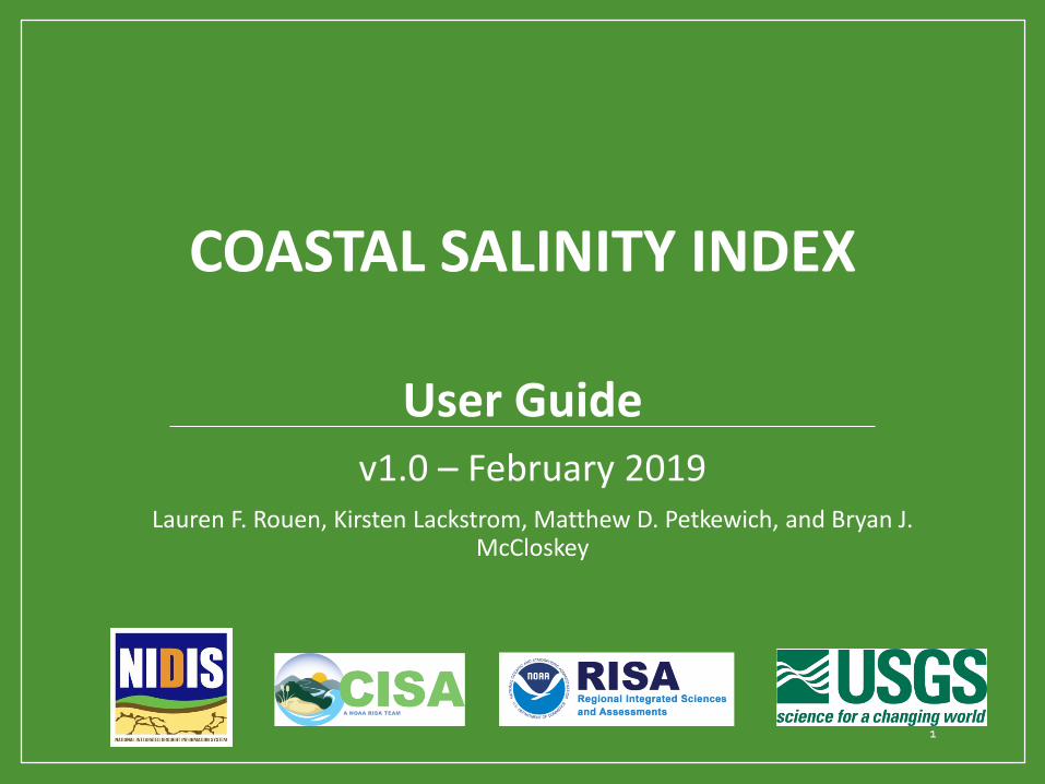
Photograph credits: Green, Chandler and Carolina Integrated Sciences and Assessments. Flying Ahead of Troubled Waters (published August 8, 2016). https://www.youtube.com/watch?v=6DS9bWMsBNM

What is the Coastal Salinity Index (CSI)?

• The CSI is a drought index tool that uses salinity data to characterize saline (drought) and freshwater (wet) conditions in coastal surface waters.

• The CSI uses an approach similar to the Standardized Precipitation Index (SPI) to show the probability of recording a given amount of salinity.

• The CSI can be computed for multiple time intervals from 1 to 24 months to characterize short- and long-term conditions.

• The CSI does not depict hourly to daily salinity fluctuations, but the response to monthly (and longer) precipitation and streamflow conditions.

decreasing salinity

4

Why was the Coastal Salinity Index (CSI) developed?

• Droughts uniquely affect coastal ecosystems and water resources through changes in salinity conditions and the location of the freshwater-saltwater interface.

• Commonly-used drought indices use inputs such as precipitation volume, streamflow, temperature, evaporation, and soil moisture conditions, but these indices do not capture the changing salinity dynamics that affect coastal areas during drought.

• The CSI was developed as a tool to monitor changing salinities in coastal surface water bodies and associated effects on estuarine habitats and freshwater availability for ecological, municipal, and industrial needs.

Conrads, P.A., Rodgers, K.D., Passeri, D.L., Prinos, S.T., Smith, C., Swarzenski, C.M., and Middleton, B.A., 2018, Coastal estuaries and lagoons—The delicate balance at the edge of the sea: U.S. Geological Survey Fact Sheet 2018–3022, 4 p., accessed July 8, 2019, at https://doi.org/10.3133/fs20183022.

High precipitation, such as caused by storms, contributes to high flows, causing decreased salinity levels in the estuary.

Low precipitation, such as caused by drought, contributes to low river flows, causing increased salinity levels in the estuary. Wind patterns can also contribute to changes in the location of the freshwater-saltwater interface. 5

-3 -2 -1 0 1 2 3

• Monthly mean salinity data are fit to a gamma distribution

and then normalized (mean of zero and standard deviation

of one).

• Index values are standard deviations from the normalized

mean values.

• An index value of zero indicates historical mean salinity.

• Negative and positive values represent increasingly saline

and fresh conditions, respectively.

• CD: Coastal drought

• CW: Coastal wet

• SPI threshold values were used to develop the coastal

drought thresholds and designations.

How is the CSI calculated?

2 5 10 20 30 Percentile 70 80 90 95 98

4 3 2 CD1 CD0 Normal CW0 CW1 2 3 4

Reference: Conrads and Darby, 2017

6

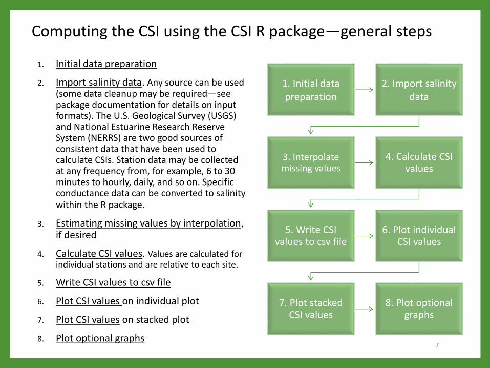
Computing the CSI using the CSI R package—general steps

1. Initial data preparation

2. Import salinity data. Any source can be used (some data cleanup may be required—see package documentation for details on input formats). The U.S. Geological Survey (USGS) and National Estuarine Research Reserve System (NERRS) are two good sources of consistent data that have been used to calculate CSIs. Station data may be collected at any frequency from, for example, 6 to 30 minutes to hourly, daily, and so on. Specific conductance data can be converted to salinity within the R package.

3. Estimating missing values by interpolation, if desired

4. Calculate CSI values. Values are calculated for individual stations and are relative to each site.

5. Write CSI values to csv file

6. Plot CSI values on individual plot

7. Plot CSI values on stacked plot

8. Plot optional graphs

1. Initial data preparation

2. Import salinity data

3. Interpolate missing values

4. Calculate CSI values

5. Write CSI values to csv file

6. Plot individual CSI values

7. Plot stacked CSI values

8. Plot optional graphs

7

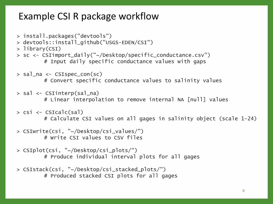
Example CSI R package workflow

> install.packages("devtools")> devtools::install_github("USGS-EDEN/CSI")> library(CSI)> sc <- CSIimport_daily("~/Desktop/specific_conductance.csv")

# Input daily specific conductance values with gaps

> sal_na <- CSIspec_con(sc)# Convert specific conductance values to salinity values

> sal <- CSIinterp(sal_na) # Linear interpolation to remove internal NA [null] values

> csi <- CSIcalc(sal) # Calculate CSI values on all gages in salinity object (scale 1-24)

> CSIwrite(csi, "~/Desktop/csi_values/") # Write CSI values to CSV files

> CSIplot(csi, "~/Desktop/csi_plots/") # Produce individual interval plots for all gages

> CSIstack(csi, "~/Desktop/csi_stacked_plots/") # Produced stacked CSI plots for all gages

8

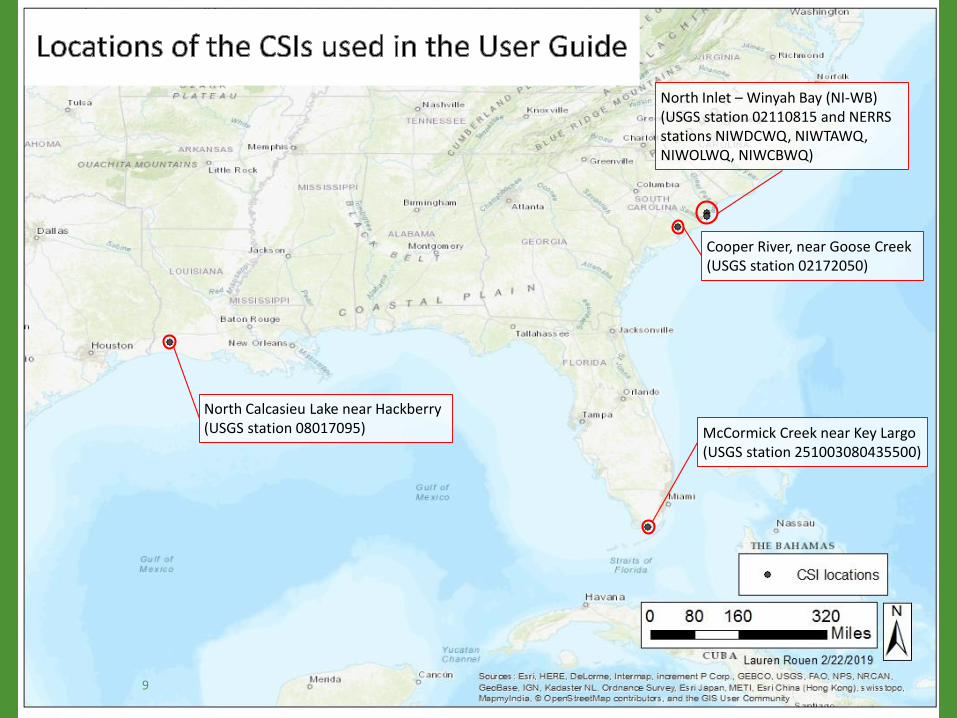
North Calcasieu Lake near Hackberry(USGS station 08017095)

North Inlet – Winyah Bay (NI-WB) (USGS station 02110815 and NERRS stations NIWDCWQ, NIWTAWQ, NIWOLWQ, NIWCBWQ)

McCormick Creek near Key Largo(USGS station 251003080435500)

Cooper River, near Goose Creek(USGS station 02172050)

9

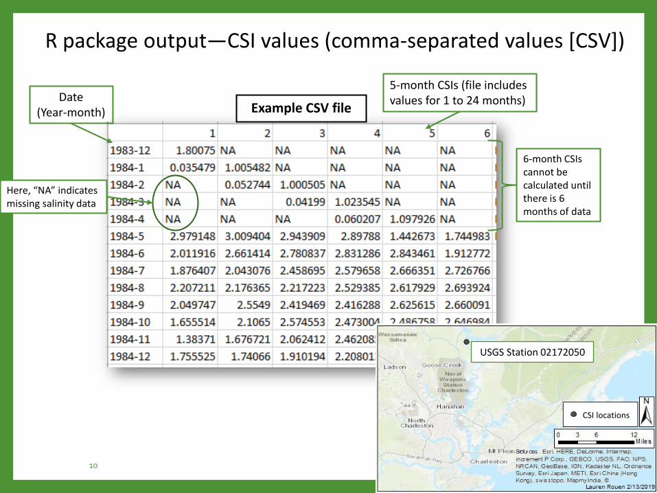
R package output—CSI values (comma-separated values [CSV])

Example CSV fileDate

(Year-month)

5-month CSIs (file includes values for 1 to 24 months)

Here, “NA” indicates missing salinity data

6-month CSIs cannot be calculated until there is 6 months of data

USGS Station 02172050

CSI locations

10

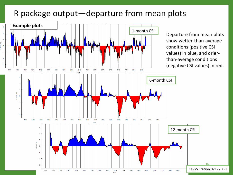
R package output—departure from mean plotsExample plots

1-month CSIDeparture from mean plots show wetter-than-average conditions (positive CSI values) in blue, and drier-than-average conditions (negative CSI values) in red.

6-month CSI

12-month CSI

USGS Station 02172050

11

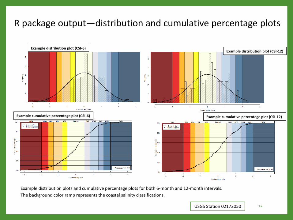
R package output—distribution and cumulative percentage plots

Example distribution plots and cumulative percentage plots for both 6-month and 12-month intervals.

The background color ramp represents the coastal salinity classifications.

USGS Station 02172050

Example distribution plot (CSI-6)Example distribution plot (CSI-12)

Example cumulative percentage plot (CSI-6) Example cumulative percentage plot (CSI-12)

12

Creating a stacked CSI plot—step by step

The CSI plots shown here and for the following “Creating a stacked CSI plot” examples are from McCormick Creek, USGS station 251003080435500, near Key Largo.

• The stacked plot combines all interval plots (from 1 to 24 months) on one plot.

• The left Y-axis shows the computational intervals.

24-month plot

12-month plot

1-month plot Stacked plot24-

12-

1-

CSI locations

13

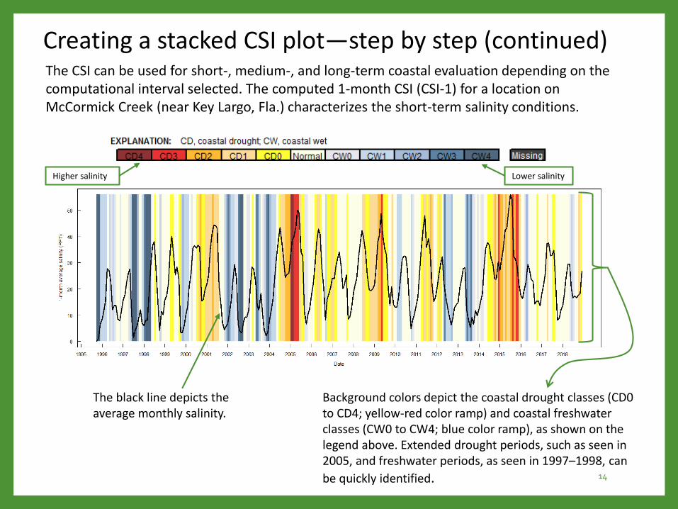
Creating a stacked CSI plot—step by step (continued)The CSI can be used for short-, medium-, and long-term coastal evaluation depending on the computational interval selected. The computed 1-month CSI (CSI-1) for a location on McCormick Creek (near Key Largo, Fla.) characterizes the short-term salinity conditions.

The black line depicts the average monthly salinity.

Lower salinityHigher salinity

Background colors depict the coastal drought classes (CD0 to CD4; yellow-red color ramp) and coastal freshwater classes (CW0 to CW4; blue color ramp), as shown on the legend above. Extended drought periods, such as seen in 2005, and freshwater periods, as seen in 1997–1998, can

be quickly identified. 14

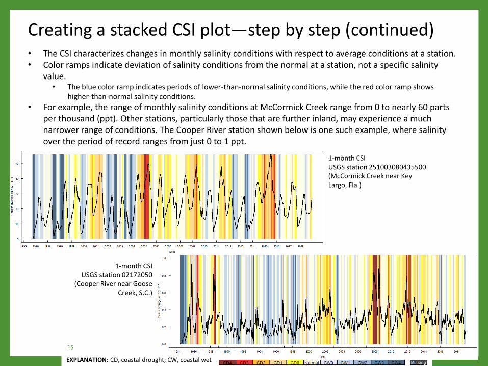
Creating a stacked CSI plot—step by step (continued)• The CSI characterizes changes in monthly salinity conditions with respect to average conditions at a station. • Color ramps indicate deviation of salinity conditions from the normal at a station, not a specific salinity

value. • The blue color ramp indicates periods of lower-than-normal salinity conditions, while the red color ramp shows

higher-than-normal salinity conditions.

• For example, the range of monthly salinity conditions at McCormick Creek range from 0 to nearly 60 parts per thousand (ppt). Other stations, particularly those that are further inland, may experience a much narrower range of conditions. The Cooper River station shown below is one such example, where salinity over the period of record ranges from just 0 to 1 ppt.

1-month CSIUSGS station 251003080435500 (McCormick Creek near Key Largo, Fla.)

1-month CSIUSGS station 02172050

(Cooper River near Goose Creek, S.C.)

EXPLANATION: CD, coastal drought; CW, coastal wet

15

EXPLANATION: CD, coastal drought; CW, coastal wet

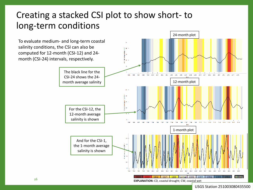
Creating a stacked CSI plot to show short- to long-term conditions

To evaluate medium- and long-term coastal salinity conditions, the CSI can also be computed for 12-month (CSI-12) and 24-month (CSI-24) intervals, respectively.

The black line for the CSI-24 shows the 24-

month average salinity

For the CSI-12, the 12-month average salinity is shown

And for the CSI-1, the 1-month average

salinity is shown

24-month plot

12-month plot

1-month plot

USGS Station 251003080435500

16

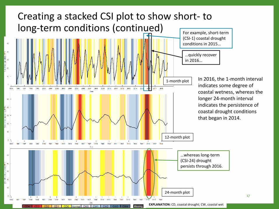
Creating a stacked CSI plot to show short- to long-term conditions (continued)

For example, short-term (CSI-1) coastal drought conditions in 2015…

…quickly recover in 2016…

…whereas long-term (CSI-24) drought persists through 2016.

24-month plot

12-month plot

1-month plot In 2016, the 1-month interval indicates some degree of coastal wetness, whereas the longer 24-month interval indicates the persistence of coastal drought conditions that began in 2014.

EXPLANATION: CD, coastal drought; CW, coastal wet

17

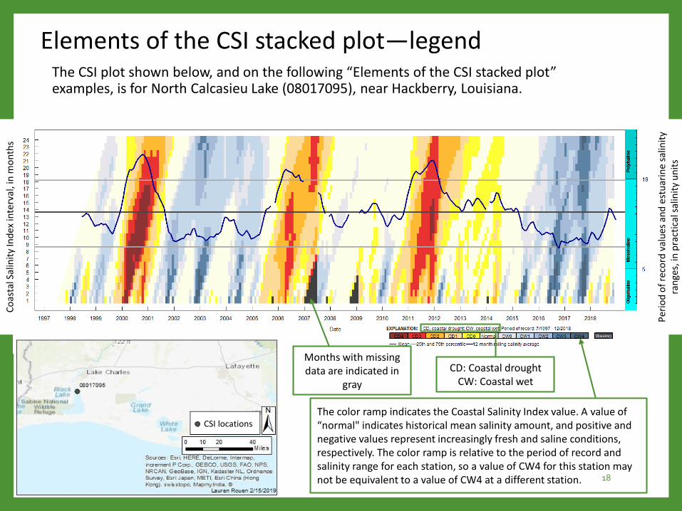
Elements of the CSI stacked plot—legend The CSI plot shown below, and on the following “Elements of the CSI stacked plot” examples, is for North Calcasieu Lake (08017095), near Hackberry, Louisiana.

Co

asta

l Sal

init

y In

dex

inte

rval

, in

mo

nth

s

Per

iod

of

reco

rd v

alu

es a

nd

est

uar

ine

salin

ity

ran

ges,

in p

ract

ical

sal

init

y u

nit

s

The color ramp indicates the Coastal Salinity Index value. A value of “normal" indicates historical mean salinity amount, and positive and negative values represent increasingly fresh and saline conditions, respectively. The color ramp is relative to the period of record and salinity range for each station, so a value of CW4 for this station may not be equivalent to a value of CW4 at a different station.

CD: Coastal droughtCW: Coastal wet

Months with missing data are indicated in

gray

CSI locations

18

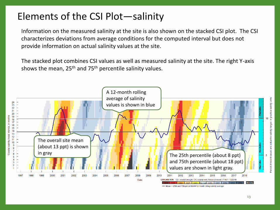
Elements of the CSI Plot—salinity Information on the measured salinity at the site is also shown on the stacked CSI plot. The CSI characterizes deviations from average conditions for the computed interval but does not provide information on actual salinity values at the site.

The stacked plot combines CSI values as well as measured salinity at the site. The right Y-axis shows the mean, 25th and 75th percentile salinity values.

A 12-month rolling average of salinity values is shown in blue

The overall site mean (about 13 ppt) is shown in gray The 25th percentile (about 8 ppt)

and 75th percentile (about 18 ppt) values are shown in light gray.

19

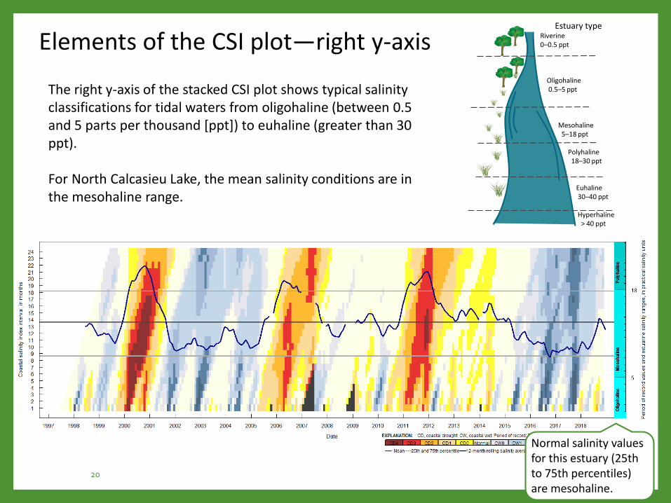
Elements of the CSI plot—right y-axis

The right y-axis of the stacked CSI plot shows typical salinity classifications for tidal waters from oligohaline (between 0.5 and 5 parts per thousand [ppt]) to euhaline (greater than 30 ppt).

For North Calcasieu Lake, the mean salinity conditions are in the mesohaline range.

Normal salinity values for this estuary (25th to 75th percentiles) are mesohaline.

Estuary typeRiverine0–0.5 ppt

Oligohaline0.5–5 ppt

Mesohaline 5–18 ppt

Polyhaline18–30 ppt

Euhaline30–40 ppt

Hyperhaline> 40 ppt

20

Reading the CSI stacked plot

The arrow indicates a period when short-term conditions were fresh, but long-term CSI values indicate drought conditions. The short-term conditions indicate a recovery from longer-term drought conditions.

The wet period that began in 2015 led to long-term wet conditions.

These were some of the driest conditions (CD4) experienced by this station over its history.

The CSI values shown here (CW4) indicate that these were some of the wettest conditions experienced by this station over its history.

Gray indicates missing salinity data in the original record. CSI values cannot be calculated. Average salinity values also

cannot be calculated, indicated by breaks in this line.

21

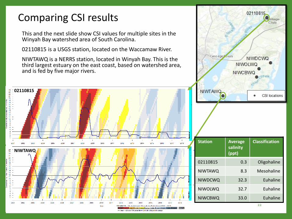
Comparing CSI results

This and the next slide show CSI values for multiple sites in the Winyah Bay watershed area of South Carolina.

02110815 is a USGS station, located on the Waccamaw River.

NIWTAWQ is a NERRS station, located in Winyah Bay. This is the third largest estuary on the east coast, based on watershed area, and is fed by five major rivers.

Station Average salinity (ppt)

Classification

02110815 0.3 Oligohaline

NIWTAWQ 8.3 Mesohaline

NIWDCWQ 32.3 Euhaline

NIWOLWQ 32.7 Euhaline

NIWCBWQ 33.0 Euhaline

NIWTAWQ

02110815

22

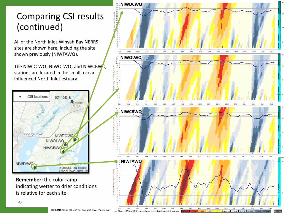
Comparing CSI results (continued)

Remember: the color ramp indicating wetter to drier conditions is relative for each site.

NIWOLWQ

NIWCBWQ

NIWTAWQ

All of the North Inlet-Winyah Bay NERRS sites are shown here, including the site shown previously (NIWTAWQ).

The NIWDCWQ, NIWOLWQ, and NIWCBWQ stations are located in the small, ocean-influenced North Inlet estuary.

NIWDCWQ

EXPLANATION: CD, coastal drought; CW, coastal wet

23

Selected references

Conrads, P.A., and Darby, L.S., 2017, Development of a Coastal Drought Index using salinity data: Bulletin of the American Meteorological Society, v. 98, no. 4, p. 753–766, accessed July 8, 2019, at https://doi.org/10.1175/BAMS-D-15-00171.1.

Conrads, P.A., Rodgers, K.D., Passeri, D.L., Prinos, S.T., Smith, C., Swarzenski, C.M., and Middleton, B.A., 2018, Coastal estuaries and lagoons—The delicate balance at the edge of the sea: U.S. Geological Survey Fact Sheet 2018–3022, 4 p., accessed July 8, 2019, athttps://doi.org/10.3133/fs20183022.

Petkewich, M.D., Lackstrom, K., McCloskey, B.J, Rouen, L.F., and Conrads, P.A., 2019, Coastal Salinity Index along the Gulf of Mexico and the southeastern Atlantic coast, 1983 to 2018: U.S. Geological Survey Open File Report 2019-####, ## p., https/doi.org/###.

• Coastal Salinity Index (CSI) GitHub, https://github.com/USGS-EDEN/CSI

• CSI R package

• The National Integrated Drought Information System (NIDIS) Coastal Carolinas Drought Early Warning System (DEWS), https://www.drought.gov/drought/dews/coastal-carolinas

• Information about the NIDIS program and projects in the Coastal Carolinas

• Conrads, P.A., 2016, Development of a Coastal Drought Index using salinity data: U.S. Geological Survey data release, accessed July 8, 2019, at https://doi.org/10.5066/F7TD9VDB. • U.S. Geological Survey data release that contains all supporting data for the Conrads and Darby (2017) article documenting the development of the CSI. It

provides CSI values for the Hagley Landing and Little Back River stations.

• Petkewich , M.D., McCloskey, B.J, Rouen, L.F., and Conrads, P.A., 2019, Coastal Salinity Index for Monitoring Drought: U.S. Geological Survey data release, accessed July 8, 2019, at https://doi.org/10.5066/P9MQLNL2. • CSI values for 97 stations through September 30, 2018

• USGS Coastal Everglades Depth Estimation Network (EDEN), https://sofia.usgs.gov/eden/coastal.php

• Real-time CSI values for South Florida locations within the EDEN

• USGS South Atlantic Water Science Center (SAWSC), www2.usgs.gov/water/southatlantic/projects/coastalsalinity/home.php

• Real-time CSI values for select stations in North Carolina, South Carolina, and Georgia

Resources

24

Acknowledgments

The CSI Team—Matthew Petkewich1, Bryan McCloskey2, Kirsten Lackstrom3, Lauren Rouen3

• 1U.S. Geological Survey

• 2Cherokee Nation Technology Solutions

• 3Carolinas Integrated Sciences and Assessments (CISA)

Funding and other support

• National Oceanic and Atmospheric Administration National Integrated Drought Information System

• National Oceanic and Atmospheric Administration Regional Integrated Sciences and Assessments

• U.S. Army Corps of Engineers, Jacksonville District

• U.S. Geological Survey Greater Everglades Priority Ecosystems Program

25