Embed Size (px)
Citation preview
June 2008Olav Bolland, EPT
Master of Science in Energy and EnvironmentSubmission date:Supervisor:
Norwegian University of Science and TechnologyDepartment of Energy and Process Engineering
CO2 Capture from Coal fired PowerPlants
Tore DugstadEsben Tonning Jensen

Problem DescriptionBackground and objective
There is an increasing interest in CO2 capture and storage as a measure to reduce man-madeemissions of the greenhouse gas CO2. Several methods have been proposed for how to do CO2capture from power plants, both for natural gas and coal. Looking ahead in time, the mostabundant fossil fuel source is coal. It is likely that in the long-term (decades), coal will be the mainprimary energy source globally for generating electricity. The emission of CO2 from coal-firedpower plants is in the range 700-1300 g CO2/KWh. This is about 2-3 times that of natural gas firedplants. It is very important to acknowledge the importance of coal and not to think that it is anenergy source of the past. For CO2 capture, coal-fired power plants will be very important to focuson, both from the perspective of the amounts of CO2 that will be emitted form such plants, butalso from the fact that the CO2 capture cost is low compared to most other large scaletechnologies, including gas fired power plants. An additional effect of CO2 capture is that in plantswhere CO2 is to be captured, a number of other pollutants can be or have to be reduced as well.
The main area of this investigation will process modelling and simulations, using a tool like HYSYSor PRO/II. The process to be studied is the IGCC (Integrated Gasification Combined Cycle). Thisprocess involves the conversion of the coal energy into a combustible gas that is fed to a gasturbine. The CO2 capture is accomplished as a process step before the combustion of the coal-derived fuel gas.
The project work will be done as cooperation between the two students involved, and only onereport is to be written. The work is to be split so that each student has the responsibility ofdifferent sub-tasks. However, for the report, with the results, the conclusions and in generalquality assurance, both students shall be equally responsible.
One of the candidates shall look into an equilibrium model of coal gasification, and bring that intoa general simulation model. This model has to cover a broad variety of coal compositions, andshould also cover dry-feed and slurry-feed gasifiers.
The other candidate shall look into modelling of an air separation unit, which purpose is to feedoxygen to the gasifier. The model must cover both low and high-pressure air separation units, aswell as LOX and GOX.
Other models, like syngas coolers or quenchers, shift reactors, CO2 capture units, gas turbine andsteam turbine modelling will to a large extent be obtained from previous work at NTNU. However,the students shall integrate the sub-models into a total plant model.
The goal of the project is to make a workable model of and IGCC with CO2 capture, that is able togive a detailed heat and mass balance, as well be able to predict sensitivities of various key

CO2 Capture from Coal fired Power Plants i
Foreword
This master thesis is a co-operation between two master students. The intention was to study a
coal fired power plant with CO2 capture. We think carbon dioxide removal from power
production will play a major role in the years to come according to limit human caused global
warming. We wanted to learn more about the different processes in a power plant and how to
optimize production under a carbon dioxide capture restriction.
The power plant explored and simulated is an Integrated Gasification Combined Cycle
(IGCC) power plant. Coal is reacted with steam and oxygen in a partial combustion and CO2
is removed from the gasified coal before combustion. The main emphasis was placed on
simulations of a gasification unit and production of oxygen to the gasifier. In addition the CO2
capture unit and power island was studied to be get complete IGCC calculations.
To solve the described task a lot of effort were put in studying literature and reports on similar
processes. The subjects of gasification and air separation were new to us and the learning
curve became steep. We found out that collection of relevant information is difficult due to
industry secrets and the fact that there are very few actual IGCC plants in the world.
Through a thorough literature study and computer simulations our understanding of the
processes grew. We feel that we have gained a lot of knowledge about IGCC and its involved
processes. At the same time we realize that the subject is very wide and to look deeply into
every part and every process probably would take a lifetime. In the end we are very satisfied
with the finished product.
There are some persons we would like to give credit for helping us completing the thesis. First
of all we would like to thank our supervisor professor Olav Bolland and co-supervisor Rahul
Anantharaman. Gasification specialist professor Øyvind Skreiberg, MatLab specialist Kjell
Kolsaker, Yasser Ahmed at the Simsci helpdesk and the members of Group Bolland has also
given us helpful information during the development of the report.
Esben Tonning Jensen Tore Dugstad
CO2 Capture from Coal fired Power Plants ii
Abstract
Coal is the most common fossil resource for power production worldwide and generates 40%
of the worlds total electricity production. Even though coal is considered a pollutive resource,
the great amounts and the increasing power demand leads to extensive use even in new
developed power plants. To cover the world's future energy demand and at the same time
limit our effect on global warming, coal fired power plants with CO2 capture is probably a
necessity.
An Integrated Gasification Combined Cycle (IGCC) Power Plant is a utilization of coal which
gives incentives for CO2 capture. Coal is partially combusted in a reaction with steam and
pure oxygen. The oxygen is produced in an air separation process and the steam is generated
in the Power Island. Out of the gasifier comes a mixture of mainly H2 and CO. In a shift
reactor the CO and additional steam are converted to CO2 and more H2. Carbon dioxide is
separated from the hydrogen in a physical absorption process and compressed for storage.
Hydrogen diluted with nitrogen from the air separation process is used as fuel in a combined
cycle similar to NGCC. A complete IGCC Power Plant is described in this report.
The air separation unit is modeled as a Linde two column process. Ambient air is compressed
and cooled to dew point before it is separated into oxygen and nitrogen in a cryogenic
distillation process. Out of the island oxygen is at a purity level of 95.6% and the nitrogen has
a purity of 99.6%. The production cost of oxygen is 0.238 kWh per kilogram of oxygen
delivered at 25°C and 1.4bar. The oxygen is then compressed to a gasification pressure of
42bar.
In the gasification unit the oxygen together with steam is used to gasify the coal. On molar
basis the coal composition is 73.5% C, 22.8% H2, 3.1% O2, 0.3% N2 and 0.3% S. The
gasification temperature is at 1571°C and out of the unit comes syngas consisting of 66.9%
CO, 31.1% H2, 1.4% H2O, 0.3% N2, 0.2% H2S and 0.1% CO2. The syngas is cooled and fed
to a water gas shift reactor. Here the carbon monoxide is reacted with steam forming carbon
dioxide and additional hydrogen. The gas composition of the gas out of the shift reactor is on
dry basis 58.2% H2, 39.0% CO2, 2.4% CO, 0.2% N2 and 0.1% H2S. Both the gasification
process and shift reactor is exothermal and there is no need of external heating. This leads to
CO2 Capture from Coal fired Power Plants iii
an exothermal heat loss, but parts of this heat is recovered. The gasifier has a Cold Gas
Efficiency (CGE) of 84.0%.
With a partial pressure of CO2 at 15.7 bar the carbon dioxide is easily removed by physical
absorption. After separation the solvent is regenerated by expansion and CO2 is pressurized to
110bar to be stored. This process is not modeled, but for the scrubbing part an energy
consumption of 0.08kWh per kilogram CO2 removed is assumed. For the compression of
CO2, it is calculated with an energy consumption of 0.11kWh per kilogram CO2 removed.
Removal of H2S and other pollutive unwanted substances is also removed in the CO2
scrubber.
Between the CO2 removal and the combustion chamber is the H2 rich fuel gas is diluted with
nitrogen from the air separation unit. This is done to increase the mass flow through the
turbine. The amount of nitrogen available is decided by the amount of oxygen produced to the
gasification process. Almost all the nitrogen produced may be utilized as diluter except from a
few percent used in the coal feeding procedure to the gasifier. The diluted fuel gas has a
composition of 50.4% H2, 46.1% N2, 2.1% CO and 1.4% CO2.
In the Power Island a combined cycle with a gas turbine able to handle large H2 amounts is
used. The use of steam in the gasifier and shift reactor are integrated in the heat recovery
steam generator (HRSG) in the steam cycle. The heat removed from the syngas cooler is also
recovered in the HRSG.
The overall efficiency of the IGCC plant modeled is 36.8%. This includes oxygen and
nitrogen production and compression, production of high pressure steam used in the
Gasification Island, coal feeding costs, CO2 removal and compression and pressure losses
through the processes. Other losses are not implemented and will probably reduce the
efficiency.
CO2 Capture from Coal fired Power Plants iv
Sammendrag
Kull er den mest utbredte fossile ressursen for kraftproduksjon i verden og står for 40% av
verdens elektrisitetsproduksjon. Selv om kull er betraktet som en forurensende ressurs,
medfører den store tilgjengeligheten samt verdens økende energibehov til utstrakt bruk også i
nye kraftverk. For å dekke verdens fremtidige energibehov samtidig som vår påvirkning på
global oppvarming begrenses, er kullkraftverk med CO2 innfangning sannsynligvis en
nødvendighet.
Et Integrated Gasification Combined Cycle (IGCC) kraftverk er en utnyttelse av kull som gir
insentiver for CO2 innfangning. Kull reagerer med damp og rent oksygen i en partiell
forbrenning. Oksygen er fremstillet i en luftseparasjonsprosess og dampen er produsert i
kraftsyklusen. Etter gassifiseringen er brenselet en blanding av hovedsakelig H2 og CO. I en
shift reaktor er CO og tilført damp konvertert til CO2 og mer H2. Karbondioksid blir skillet fra
hydrogenet i en fysisk absorpsjonsprosess og komprimert for lagring. Hydrogen fortynnet
med nitrogen fra luftseparasjonsprosessen er brukt som brensel i en kombinert gass- og
dampsyklus tilsvarende som for gasskraftverk. Et komplett IGCC anlegg er presentert i denne
rapport.
Luftseparasjonsenheten modellert tilsvarer Lindes dobbel-kolonne prosess. Luft er
komprimert og kjølnet til duggpunkt før den er separert til oksygen og nitrogen i en
kryogenisk destillasjonsprosess. Ut av enheten kommer oksygen med en renhet på 95.6% og
nitrogen med en renhet på 99.6%. Oksygenets produksjonskostnad er på 0.238kWh per
kilogram oksygen levert ved 25°C og 1.4bar. Oksygenet er deretter komprimert til et
gassifiseringtrykk på 42bar.
I gasifiseringsenheten er oksygen brukt sammen med damp til å gassifisere kull. Kullet har på
molar basis følgende sammensetning, 73.5% C, 22.8% H2, 3.1% O2 og 0.3% av henholdsvis
N2 og S. Gasifiseringen skjer ved 1571°C og ut av prosessen kommer syngas bestående av
66.9% CO, 31.1% H2, 1.4% H2O, 0.3% N2, 0.2% H2S and 0.1% CO2. Gassen er kjølnet og
sendt til en shift reaktor. Her reagerer karbonmonoksidet med damp og danner karbondioksid
og hydrogen. Sammensetningen av gassen ut av shift reaktoren er på tørr basis 58.2% H2,
39.0% CO2, 2.4% CO, 0.2% N2 og 0.1% H2S. Både gasifiserings- og shiftprosessen er
CO2 Capture from Coal fired Power Plants v
eksoterme og har ikke behov for ekstern varmetilførsel. Dette fører til et eksotermt varmetap,
men deler av varmen er gjenvunnet. Gasifiseringsprosessen har en gasifiseringsvirkningsgrad
(CGE) på 84.0%.
Med et partielltrykk på 15.7bar er det relativt enkelt å skille CO2 fra brenselsgassen ved fysisk
absorpsjon. Etter separasjonen er løsningsmiddelet regenerert ved ekspansjon og
karbondioksidet er komprimert til lagringstrykk på 110bar. Denne prosessen er ikke
modellert, men for utskillelsesprosessen er det antatt et energiforbruk på 0.08kWh per
kilogram CO2 fjernet. For kompresjonsarbeidet er det regnet med et energiforbruk på
0.11kWh per kilogram CO2 fjernet. Innfangning av H2S og andre forurensende uønskede
stoffer er også fjernet i denne enheten.
Mellom CO2 fjerningen og brennkammeret er den hydrogenrike brenselsgassen fortynnet med
nitrogen fra luftseparasjonsenheten. Dette er gjort for å øke massestrømmen gjennom
turbinen. Mengden tilgjengelig nitrogen er bestemt av oksygenbehovet i gasifiseringsenheten.
Sett bort fra et par prosent nitrogen brukt i fødeprosedyren for kull til gasifiseringsenheten,
kan all nitrogenet brukes som brenselsgassfortynner. Den fortynnede brenselsgassen har
følgende sammensetning, 50.4% H2, 46.1% N2, 2.1% CO og 1.4% CO2.
I kraftprosessen er det brukt en gassturbin som håndterer høyt innhold av hydrogen i
brenselet. Bruken av damp i gasifiserings- og shiftprosessen er integrert i Heat Recovery
Steam Generatoren (HRSG) i dampsyklusen. Varmen fjernet i syngaskjølingen er også
gjenvunnet i HRSG.
Den totale virkningsgraden for IGCC kraftverket modellert er på 36.8%. Dette inkluderer
oksygen og nitrogen produksjon og kompresjon, produksjon av høytrykks damp brukt i
gasifiseringen, kullfødekostnader, CO2 innfangning og kompresjon og trykktap gjennom
prosessene. Andre tap er ikke medregnet og vil sannsynligvis redusere virkningsgraden
ytterligere.
CO2 Capture from Coal fired Power Plants vi
Index
Foreword……………………………………………………………………………………….i
Abstract………………………………………………………………………………………..ii
Sammendrag………………………………………………………………………………….iv
Index…………………………………………………………………………………………..vi
Figure Index……………………………………………………………………………….…ix
Table Index…………………………………………………………………………………...xi
Abbreviations……………………………………………………………………………….xiii
1 Introduction…………………………………………………………………………...1
1.1 CO2 emissions………………………………………………………………….1
1.2 Coal fired power plants…..………………………………...………..…………2
1.3 Integrated Gasification Combined Cycle………………….…………..……….4
2 Theoretical Background………………………….………………………………...…6
2.1 Air Separation Island……...…………………………………….………..……..6
2.1.1 Distillation theory………………………………………………..……...6
2.1.2 Air separation unit……………………………………………………...16
2.2 Gasification Island.…………………………………………………..………...30
2.2.1 Coal…………………………………………………………………….30
2.2.2 Gasification…………………………………………………………….34
2.2.3 Gasification procedures…………………………………………….….41
2.3 Acid Gas Removal………………………………………………….…...……..52
2.3.1 Properties and technologies…………………………………………….52
2.3.2 Removal of H2S and CO2 in IGCC…………………………………….54
2.4 Power Island………………………………………………………………....…58
2.4.1 Introduction…………………………………………………………….58
2.4.1 Turbines fired with syngas……………………………………………..59
2.4.2 Turbines fired with hydrogen only…………………………………….62
2.5 IGCC Power Plant……………………………………………………………...64
2.5.1 Integration of processes………………………………………………...64
2.5.2 Energy efficiency……………………………………………………….66
CO2 Capture from Coal fired Power Plants vii
3 Method………………………………………………………………………………...67
3.1 Air Separation Island……………………………………………………….…..67
3.1.1 Simulation tool…………………………………………………………67
3.1.2 Gaseous oxygen………………………………………………………...67
3.1.3 Liquid oxygen…………………………………………………………..80
3.1.4 Argon treatment………………………………………………………...83
3.2 Gasification Island……………………………………………………………...84
3.2.1 Simulation tools………………………………………………………...84
3.2.2 MatLab calculations……………………………………………………84
3.2.3 PRO/II testing…………………………………………………………..90
3.2.4 PRO/II simulations……………………………………………………. 95
3.2.5 Chemical equilibrium calculator……………………………………...102
3.2.6 Water shift reforming………………………………………………....103
3.3 Acid Gas Removal……………………………………...……………….……107
3.3.1 Simulation tool………………………………………………………..107
3.3.2 CO2 capture unit………………………………………………………107
3.3.3 H2S capture unit………………………………………………………109
3.4 Power Island…………………………………..………………………..……..111
3.4.1 Simulation tool………………………………………………………..111
3.4.2 Gas Turbine…………………………………………………………...111
3.4.3 HRSG and Steam Turbine…………………………………………….114
3.5 IGCC Power Plant………….......……….…………………………….………117
3.5.1 Integrating the whole plant……………………………………………117
CO2 Capture from Coal fired Power Plants viii
4 Results and discussion………………………………………………………………118
4.1 Air Separation Island…………………………………………………………118
4.1.1 Gaseous oxygen………………………………………………………118
4.1.2 Liquid oxygen…………………………………………………………135
4.2 Gasification Island………………………………………………………...….138
4.2.1 Introduction………………………………………………………...…138
4.2.2 MatLab calculations………………………………………………..…138
4.2.3 PRO/II simulations…………………………………………………....139
4.2.4 Equilibrium calculator………………………………………………...146
4.2.5 Water shift reforming…………………………………………………148
4.3 Acid Gas Removal……………………………………………………………152
4.3.1 Considerations………………………………………………………...152
4.4 Power Island…………………………………………………………………..153
4.4.1 Gas Turbine…………………………..……………………………….153
4.4.2 HRSG and Steam Turbine…………..………………………………...156
4.4.3 Overall view of the Power Island……………………………………..159
4.5 IGCC Power Plant………………………………………………………….…161
4.5.1 Initial calculation…………………………………………………..….161
4.5.2 Deviation from initial calculation……………………………………..163
4.5.3 Main number in favourable units………………………………..……165
5 Conclusion…………………………………………………………………………...166
6 Reference list………………………………………………………………………...168
Appendix……………………………………………………………………………………..171
CO2 Capture from Coal fired Power Plants ix
Figure Index
Figure 1.1. Rankine Cycle.……………………………………………………………………..2
Figure 1.2. Combined Cycle, Brayton and Rankine…………………………………………...3
Figure 1.3. Overview of the main processes in an IGCC Power Plant………………………...4
Figure 2.1. Vapor-liquid separation…………………………………………………………....9
Figure 2.2. Distillation column with condenser and reboiler…………………………………10
Figure 2.3. Rectifier section………………………………………………………………..…11
Figure 2.4. Stripping section………………………………………………………………….12
Figure 2.5. Feed tray………………………………………………………………………….13
Figure 2.6. McCabe Thiele diagram………………………………………………………….15
Figure 2.7. Air separation unit………………………………………………………………..16
Figure 2.8. Main heat exchanger……………………………………………………………...20
Figure 2.9. High pressure column…………………………………………………………….22
Figure 2.10. Low pressure column……………………………………………………………23
Figure 2.11. Combined condenser and reboiler………………………………………………24
Figure 2.12. Air separation unit with after treatment………………………………………...26
Figure 2.13. Liquid oxygen plant…………………………………………………………….27
Figure 2.14. GOX plant with argon treatment………………………………………………..29
Figure 2.15. Transforming coal to syngas……………………………………………………33
Figure 2.16. Influence of heating rate………………………………………………………...34
Figure 2.17. Gasification process……………………………………………………………..35
Figure 2.18. Input and output in a water gas shift reactor…………………………………….40
Figure 2.19. Lurgi Dry Ash Gasifier………………………………………………………….43
Figure 2.20. Top-Fired Dry Coal Feed Slagging Entrained-Flow Gasifier…………………..45
Figure 2.21. Sour water gas shift reaction……………………………………………………54
Figure 2.22. Sweet water gas shift reaction…………………………………………………..55
Figure 3.1. Model of air compressor……………………………………………………….…69
Figure 3.2. Model of the main heat exchanger………………………………………………..71
Figure 3.3. Separation factor for the high pressure column…………………………………..73
Figure 3.4. Model of high pressure column…………………………………………………..74
Figure 3.5. Model of low pressure column…………………………………………………...75
Figure 3.6. Model of combined condenser and reboiler……………………………………...76
CO2 Capture from Coal fired Power Plants x
Figure 3.7. Model of subcooler…………………………………………………………….…78
Figure 3.8. Model of GOX plant without oxygen compression………………………..……..79
Figure 3.9. Model of LOX plant………………………………………………………….…..80
Figure 3.10. Gasification Island………………………………………………………..……..91
Figure 3.11. Model of a gasifier………………………………………………………...…….98
Figure 3.12. Product stream at normal conditions……………………………………………98
Figure 3.13. Model of a slurry feed gasifier………………………………………………...100
Figure 3.14. Two stepped water gas shift reactor………………………………………..….104
Figure 3.15. Model of Gasification Island………………………………………………..…106
Figure 3.16. AGR black box……………………………………………………………..….109
Figure 3.17. Generating steam from exhaust gas and hot syngas………………………..….115
Figure 3.18. Generating steam between the stages in the shift reactor……………………...115
Figure 3.19. Generating steam after the shift reactor……………………………………..…116
Figure 4.1. Model of GOX plant with modified main heat exchanger……………………...124
Figure 4.2. Decrease of total work with increasing compressor steps……………………....126
Figure 4.3. Separation factor for high pressure column with 11 trays……………………....129
Figure 4.4. Separation factor for low pressure column with 16 trays……………………….130
Figure 4.5. Final GOX model……………………………………………………………….134
Figure 4.6. Efficiency deviation by changed CO2 capture cost……………………………..164
CO2 Capture from Coal fired Power Plants xi
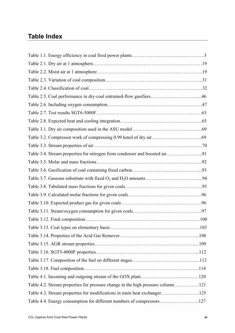
Table Index Table 1.1. Energy efficiency in coal fired power plants……………………………………….3
Table 2.1. Dry air at 1 atmosphere……………………………………………………………19
Table 2.2. Moist air at 1 atmosphere………………………………………………………….19
Table 2.3. Variation of coal composition……………………………………………………..31
Table 2.4. Classification of coal………………………………………………………………32
Table 2.5. Coal performance in dry-coal entrained-flow gasifiers…………………………...46
Table 2.6. Including oxygen consumption……………………………………………………47
Table 2.7. Test results SGT6-5000F………………………………………………………….63
Table 2.8. Expected heat and cooling integration…………………………………………….65
Table 3.1. Dry air composition used in the ASU model……………………………………...69
Table 3.2. Compressor work of compressing 0.99 kmol of dry air…………………………..69
Table 3.3. Stream properties of air……………………………………………………………70
Table 3.4. Stream properties for nitrogen from condenser and boosted air…………………..81
Table 3.5. Molar and mass fractions………………………………………………………….92
Table 3.6. Gasification of coal containing fixed carbon……………………………………...93
Table 3.7. Gaseous substitute with fixed O2 and H2O amounts……………………………....94
Table 3.8. Tabulated mass fractions for given coals………………………………………….95
Table 3.9. Calculated molar fractions for given coals………………………………………..96
Table 3.10. Expected product gas for given coals……………………………………………96
Table 3.11. Steam/oxygen consumption for given coals……………………………………..97
Table 3.12. Final composition…...………………………………………………………..…100
Table 3.13. Coal types on elementary basis…………………………………………………103
Table 3.14. Properties of the Acid Gas Remover…………………………………………...108
Table 3.15. AGR stream properties…………………………………………………………109
Table 3.16. SGT5-4000F properties………………………………………………………...112
Table 3.17. Composition of the fuel on different stages………………………………….....112
Table 3.18. Fuel composition……………………………………………………………….114
Table 4.1. Incoming and outgoing stream of the GOX plant……………………………….120
Table 4.2. Stream properties for pressure change in the high pressure column…………….121
Table 4.3. Stream properties for modifications in main heat exchanger……………………125
Table 4.4. Energy consumption for different numbers of compressors…………………….127
CO2 Capture from Coal fired Power Plants xii
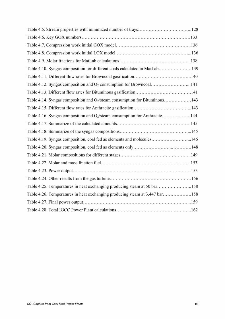
Table 4.5. Stream properties with minimized number of trays………………………….…..128
Table 4.6. Key GOX numbers………………………………………………………………133
Table 4.7. Compression work initial GOX model…………………………………………..136
Table 4.8. Compression work initial LOX model…………………………………………...136
Table 4.9. Molar fractions for MatLab calculations………………………………………...138
Table 4.10. Syngas composition for different coals calculated in MatLab………………….139
Table 4.11. Different flow rates for Browncoal gasification………………………………..140
Table 4.12. Syngas composition and O2 consumption for Browncoal……………………...141
Table 4.13. Different flow rates for Bituminous gasification……………………………….141
Table 4.14. Syngas composition and O2/steam consumption for Bituminous………………143
Table 4.15. Different flow rates for Anthracite gasification………………………………...143
Table 4.16. Syngas composition and O2/steam consumption for Anthracite……………….144
Table 4.17. Summarize of the calculated amounts………………………………………….145
Table 4.18. Summarize of the syngas compositions………………………………………...145
Table 4.19. Syngas composition, coal fed as elements and molecules……………………...146
Table 4.20. Syngas composition, coal fed as elements only……………………..………….148
Table 4.21. Molar compositions for different stages………………………………………..149
Table 4.22. Molar and mass fraction fuel…………………………………………………...153
Table 4.23. Power output……………………………………………………………………153
Table 4.24. Other results from the gas turbine………………………………………………156
Table 4.25. Temperatures in heat exchanging producing steam at 50 bar…………………..158
Table 4.26. Temperatures in heat exchanging producing steam at 3.447 bar……………….158
Table 4.27. Final power output……………………………………………………………...159
Table 4.28. Total IGCC Power Plant calculations…………………………………………..162
CO2 Capture from Coal fired Power Plants xiii
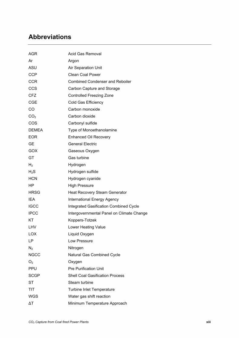
Abbreviations
AGR Acid Gas Removal
Ar Argon
ASU Air Separation Unit
CCP Clean Coal Power
CCR Combined Condenser and Reboiler
CCS Carbon Capture and Storage
CFZ Controlled Freezing Zone
CGE Cold Gas Efficiency
CO Carbon monoxide
CO2 Carbon dioxide
COS Carbonyl sulfide
DEMEA Type of Monoethanolamine
EOR Enhanced Oil Recovery
GE General Electric
GOX Gaseous Oxygen
GT Gas turbine
H2 Hydrogen
H2S Hydrogen sulfide
HCN Hydrogen cyanide
HP High Pressure
HRSG Heat Recovery Steam Generator
IEA International Energy Agency
IGCC Integrated Gasification Combined Cycle
IPCC Intergovernmental Panel on Climate Change
KT Koppers-Totzek
LHV Lower Heating Value
LOX Liquid Oxygen
LP Low Pressure
N2 Nitrogen
NGCC Natural Gas Combined Cycle
O2 Oxygen
PPU Pre Purification Unit
SCGP Shell Coal Gasification Process
ST Steam turbine
TIT Turbine Inlet Temperature
WGS Water gas shift reaction
ΔT Minimum Temperature Approach

CO2 Capture from Coal fired Power Plants xiv
Introduction
CO2 Capture from Coal fired Power Plants 1
1 Introduction
1.1 CO2 emissions
The issue of global warming has been discussed by scientists for 30 years without affecting
the public remarkable. The registered increase in temperature the last 50 years has been
explained by either natural temperature oscillations or man made greenhouse gas emissions.
In the last 10 years the relationship between greenhouse gases and global warming has
become a wide agreement among scientists. In 1997 the Kyoto Protocol was negotiated with a
common goal of the governments ratified the treaty of “achieving stabilization of greenhouse
gas concentrations in the atmosphere at a level that would prevent dangerous anthropogenic
interference with the climate system” [1].
The climate change is today admitted as a problem by almost every scientist, state leader and
random man. According to a conservative assumption by the IPCC there is a 90 percentage
possibility that the global warming originates from man made greenhouse gas emissions [2].
The major greenhouse gas emitted by humans is carbon dioxide. Carbon dioxide is a natural
end product in all kind of combustions from fossil fuel fired power plants to sparkling
firewood in the fireplace. Carbon in wood, natural gas, oil or coal reacts with oxygen and
forms carbon dioxide and water vapor.
Power production is one of the largest contributors to CO2 emissions. Combustion of coal, oil
or natural gas to produce heat and electricity leads to great emission rates of carbon dioxide.
The amount of CO2 emitted varies with type of fuel and combustion technology. Carbon rich
fuels like coal produce most CO2 per amount of energy while hydrogen rich fuels like natural
gas have smaller emissions. In this case it is advantageous to look at the m over n ratio, where
m is carbon and n is hydrogen. Under equal combustion criteria a higher m over n ratio leads
to higher CO2 emissions.
Introduction
CO2 Capture from Coal fired Power Plants 2
coal oil natural gas
m m mn n n
⎛ ⎞ ⎛ ⎞ ⎛ ⎞> >⎜ ⎟ ⎜ ⎟ ⎜ ⎟⎝ ⎠ ⎝ ⎠ ⎝ ⎠
⇒ ( ) ( ) ( )1.1 0.5 0.25coal oil natural gas
≈ > ≈ > ≈ (1.1)
Combustion of coal leads to a remarkable higher emission rate than oil or natural gas. The
exhaust gas from coal combustion contains 12-14 percent carbon dioxide while exhaust gas
from natural gas only contains 3.2-4.2 percent. In amounts this equals to 750-1100 gram per
kilowatt hour of electricity produced in a coal fired power plant compared to 300-350 gram in
a natural gas fired power plant [3] [4].
Although, the great coal resources gives coal a significant role in covering the increasing
global energy demand. And to reduce the worlds total carbon dioxide emissions the reduction
must be done where it matters, combustion of carbon rich fuels.
1.2 Coal fired Power Plants
This report focuses at coal fired power plants. Coal is the fossil fuel there is most of in the
world and it will be one of the main resources for power production in many years to come.
According to BP statistics the world need of coal is covered for 147 years [5]. To satisfy both
the increasing energy demand and the goal of the Kyoto Protocol the technology in the coal
fired power plants need to be improved.
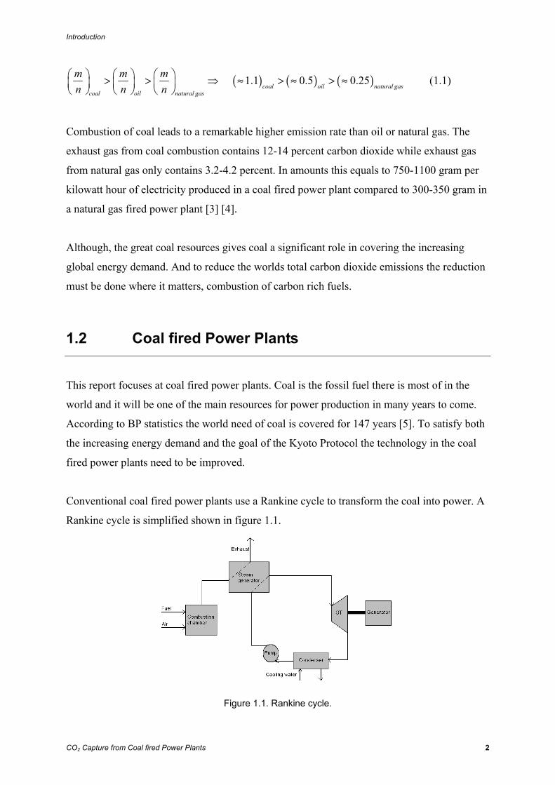
Conventional coal fired power plants use a Rankine cycle to transform the coal into power. A
Rankine cycle is simplified shown in figure 1.1.
Figure 1.1. Rankine cycle.
Introduction
CO2 Capture from Coal fired Power Plants 3
The most efficient power plants based on a Rankine cycle is the Pulverized Coal (PC) plant.
The combustion of the pulverized coal produces exhaust gas which contains CO2 that may be
captured.
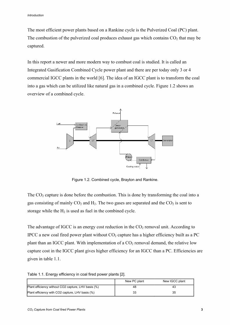
In this report a newer and more modern way to combust coal is studied. It is called an
Integrated Gasification Combined Cycle power plant and there are per today only 3 or 4
commercial IGCC plants in the world [6]. The idea of an IGCC plant is to transform the coal
into a gas which can be utilized like natural gas in a combined cycle. Figure 1.2 shows an
overview of a combined cycle.
Figure 1.2. Combined cycle, Brayton and Rankine.
The CO2 capture is done before the combustion. This is done by transforming the coal into a
gas consisting of mainly CO2 and H2. The two gases are separated and the CO2 is sent to
storage while the H2 is used as fuel in the combined cycle.
The advantage of IGCC is an energy cost reduction in the CO2 removal unit. According to
IPCC a new coal fired power plant without CO2 capture has a higher efficiency built as a PC
plant than an IGCC plant. With implementation of a CO2 removal demand, the relative low
capture cost in the IGCC plant gives higher efficiency for an IGCC than a PC. Efficiencies are
given in table 1.1.
Table 1.1. Energy efficiency in coal fired power plants [2]. New PC plant New IGCC plant
Plant efficiency without CO2 capture, LHV basis (%) 48 43
Plant efficiency with CO2 capture, LHV basis (%) 33 35
Introduction
CO2 Capture from Coal fired Power Plants 4
The efficiency in each case may have some variations with surrounding conditions and
different technologies.
Table 1.1 shows that for plants with capture of carbon dioxide IGCC has a higher efficiency
and is probably a more future oriented type of power plant.
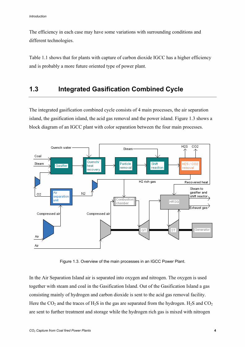
1.3 Integrated Gasification Combined Cycle
The integrated gasification combined cycle consists of 4 main processes, the air separation
island, the gasification island, the acid gas removal and the power island. Figure 1.3 shows a
block diagram of an IGCC plant with color separation between the four main processes.
Figure 1.3. Overview of the main processes in an IGCC Power Plant.
In the Air Separation Island air is separated into oxygen and nitrogen. The oxygen is used
together with steam and coal in the Gasification Island. Out of the Gasification Island a gas
consisting mainly of hydrogen and carbon dioxide is sent to the acid gas removal facility.
Here the CO2 and the traces of H2S in the gas are separated from the hydrogen. H2S and CO2
are sent to further treatment and storage while the hydrogen rich gas is mixed with nitrogen

Introduction
CO2 Capture from Coal fired Power Plants 5
from the air separation unit before entering the combustion chamber. In the Power Island
electricity is generated similar to the power cycle in a natural gas fired power plant.
This report is chronological studying these four main processes in detail. The theory behind
each process is presented before simulations and calculations are made for each island. In the
end the islands are set together in a complete IGCC Power Plant model.
Theoretical Background
CO2 Capture from Coal fired Power Plants 6
2 Theoretical Background
2.1 Air Separation Island
2.1.1 Distillation theory
A distillation column separates two or more components based on the different boiling points
for the given substances. The special case of air separation for an IGCC plant is principally to
separate oxygen and nitrogen. In addition to oxygen and nitrogen, air also contains argon,
water, carbon dioxide and traces of other substances. The traces are normally neglected while
the water and the CO2 should be removed before the distillation column. It is also a question
if the argon should be separated from oxygen and nitrogen or not. If the argon can be utilized
it may be economical beneficial to remove it.
There are several factors that influence the performance of a distillation column. The feed rate
and the feed content play a major role and will affect the design of the column. The main
property of this is the boiling point of the different substances. Small differences in boiling
point require a more advanced separation process. In the case of N2 and O2 the difference in
boiling point at 1 atmosphere is about 13˚C [7]. Argon has boiling point between oxygen and
nitrogen and removal of argon therefore complicates the process. Roughly spoken, the wanted
purity of the products (degree of separation) determines the height of the column while the
amount of feed determines the diameter [8].
In this part of the report a theoretical introduction to distillation is given. Sources for the
derivations are Humphrey [8] and Geankoplis [9]. In chapter 2.1.2 Air Separation Unit the
specific case of oxygen-nitrogen separation is further explained.
2.1.1.1 Equilibrium
Equilibrium between liquid and vapor phase is reached when no further changes in
composition, temperature or pressure occur in a fixed environment. A typical distillation
Theoretical Background
CO2 Capture from Coal fired Power Plants 7
column contains a lot of steps or trays where equilibrium conditions occur. A single step may
be studied as a tank where an external heat source heats the contents and boiling will occur.
The most volatile component will concentrate more in vapor phase while the component with
higher boiling point will concentrate in liquid phase. In a column with many trays the vapor
will move upwards to the next stage, reach å new equilibrium with the down coming liquid
and so on. Likewise the liquid will move downwards and meet the upcoming vapor. The
vapor purity at the top of the column depends on the number of equilibrium trays. This is
likewise for the liquid in the bottom.
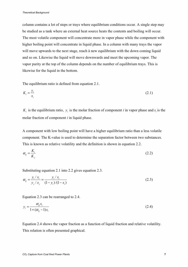
The equilibrium ratio is defined from equation 2.1.
ii
i
yKx
= (2.1)
iK is the equilibrium ratio, iy is the molar fraction of component i in vapor phase and ix is the
molar fraction of component i in liquid phase.
A component with low boiling point will have a higher equilibrium ratio than a less volatile
component. The K-value is used to determine the separation factor between two substances.
This is known as relative volatility and the definition is shown in equation 2.2.
iij
j
KK
α = (2.2)
Substituting equation 2.1 into 2.2 gives equation 2.3.
/ // (1 ) /(1 )
i i i iij
j j i i
y x y xy x y x
α = =− −
(2.3)
Equation 2.3 can be rearranged to 2.4.
1 ( 1)ij i
iij i
xy
xαα
=+ −
(2.4)
Equation 2.4 shows the vapor fraction as a function of liquid fraction and relative volatility.
This relation is often presented graphical.
Theoretical Background
CO2 Capture from Coal fired Power Plants 8
With ideal equilibrium conditions Raoult’s law may be derived.
i i ip P x= (2.5)
In equation 2.5 is ip the partial pressure of component i in the vapor while iP is the vapor
pressure of pure component i. The vapor pressure is tabulated for different substances and ix
is the molar fraction of component i in the liquid.
Another ideal law for systems of vapor and liquid is the Dalton’s law.
i ip Py= (2.6)
Here is P the total pressure. Equation 2.6 can be rearranged and combined with equation 2.5.
i i ii
p P xyP P
= = (2.7)
The same is legal for component j and using yi and yj in equation 2.3 gives 2.8 gives.
1// 1
i i
i i i iij
j jj j j
j
P xy x P x P
P xy x PP x
α = = =i
i (2.8)
From equation 2.8 the separation potential for two substances may be determined. ijα is
decided and through equation 2.4 the vapor fractions may be plotted against the liquid
fractions. Equation 2.8 gives the ijα - value for ideal conditions. For non ideal systems the
behavior is corrected with an activity coefficient γ. The expression for the relative volatility
under non ideal conditions is given in 2.9.
i iij
j j
PP
γαγ
= (2.9)
Theoretical Background
CO2 Capture from Coal fired Power Plants 9
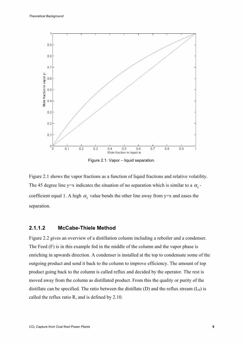
Figure 2.1. Vapor – liquid separation.
Figure 2.1 shows the vapor fractions as a function of liquid fractions and relative volatility.
The 45 degree line y=x indicates the situation of no separation which is similar to a ijα -
coefficient equal 1. A high ijα value bends the other line away from y=x and eases the
separation.
2.1.1.2 McCabe-Thiele Method
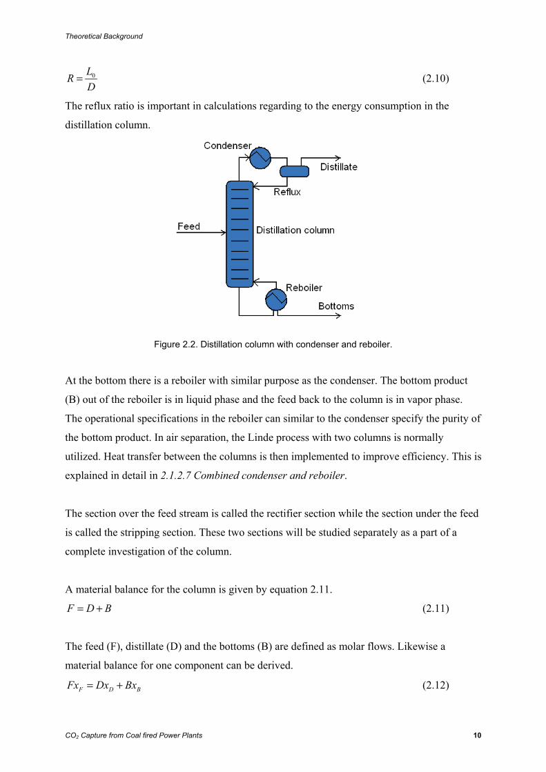
Figure 2.2 gives an overview of a distillation column including a reboiler and a condenser.
The Feed (F) is in this example fed in the middle of the column and the vapor phase is
enriching in upwards direction. A condenser is installed at the top to condensate some of the
outgoing product and send it back to the column to improve efficiency. The amount of top
product going back to the column is called reflux and decided by the operator. The rest is
moved away from the column as distillated product. From this the quality or purity of the
distillate can be specified. The ratio between the distillate (D) and the reflux stream (L0) is
called the reflux ratio R, and is defined by 2.10.
Theoretical Background
CO2 Capture from Coal fired Power Plants 10
0LRD
= (2.10)
The reflux ratio is important in calculations regarding to the energy consumption in the
distillation column.
Figure 2.2. Distillation column with condenser and reboiler.
At the bottom there is a reboiler with similar purpose as the condenser. The bottom product
(B) out of the reboiler is in liquid phase and the feed back to the column is in vapor phase.
The operational specifications in the reboiler can similar to the condenser specify the purity of
the bottom product. In air separation, the Linde process with two columns is normally
utilized. Heat transfer between the columns is then implemented to improve efficiency. This is
explained in detail in 2.1.2.7 Combined condenser and reboiler.
The section over the feed stream is called the rectifier section while the section under the feed
is called the stripping section. These two sections will be studied separately as a part of a
complete investigation of the column.
A material balance for the column is given by equation 2.11.
F D B= + (2.11)
The feed (F), distillate (D) and the bottoms (B) are defined as molar flows. Likewise a
material balance for one component can be derived.
F D BFx Dx Bx= + (2.12)
Theoretical Background
CO2 Capture from Coal fired Power Plants 11
x is the concentration of the most volatile component respectively for feed, distillate and
bottom.
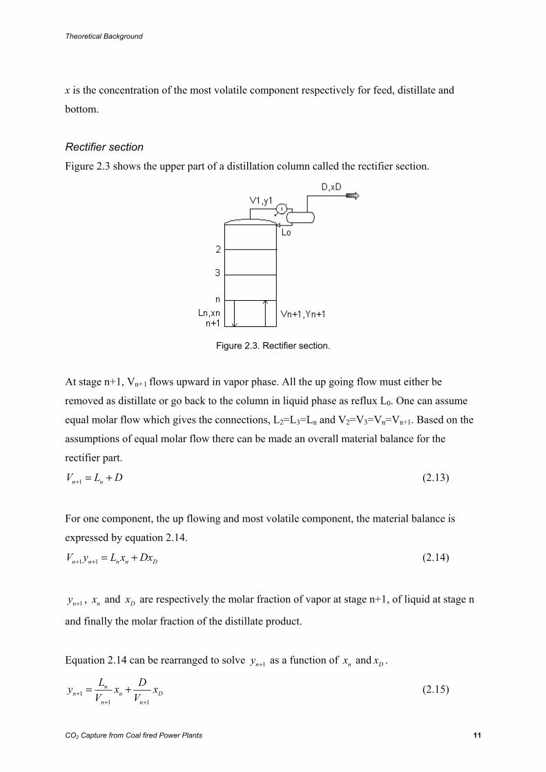
Rectifier section
Figure 2.3 shows the upper part of a distillation column called the rectifier section.
Figure 2.3. Rectifier section.
At stage n+1, Vn+1 flows upward in vapor phase. All the up going flow must either be
removed as distillate or go back to the column in liquid phase as reflux L0. One can assume
equal molar flow which gives the connections, L2=L3=Ln and V2=V3=Vn=Vn+1. Based on the
assumptions of equal molar flow there can be made an overall material balance for the
rectifier part.
1n nV L D+ = + (2.13)
For one component, the up flowing and most volatile component, the material balance is
expressed by equation 2.14.
1 1n n n n DV y L x Dx+ + = + (2.14)
1ny + , nx and Dx are respectively the molar fraction of vapor at stage n+1, of liquid at stage n
and finally the molar fraction of the distillate product.
Equation 2.14 can be rearranged to solve 1ny + as a function of nx and Dx .
11 1
nn n D
n n
L Dy x xV V+
+ +
= + (2.15)
Theoretical Background
CO2 Capture from Coal fired Power Plants 12
Rearranging equation 2.15 and using the definition of reflux ratio from equation 2.10 gives
equation 2.16 and 2.17.
1
11n
DV R+
=+
(2.16)
1 1
11 11 1
n
n n
L D RV V R R+ +
= − = − =+ +
(2.17)
Equation 2.16 and 2.17 put into equation 2.15 gives the equation for the enriching part given
in 2.18.
11
1 1n n DRy x x
R R+ = ++ +
(2.18)
This relation can be plotted in a liquid vapor diagram and it will occur as a straight line for
constant reflux ratio.
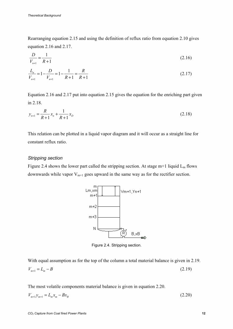
Stripping section
Figure 2.4 shows the lower part called the stripping section. At stage m+1 liquid Lm flows
downwards while vapor Vm+1 goes upward in the same way as for the rectifier section.
Figure 2.4. Stripping section.
With equal assumption as for the top of the column a total material balance is given in 2.19.
1m mV L B+ = − (2.19)
The most volatile components material balance is given in equation 2.20.
1 1m m m m BV y L x Bx+ + = − (2.20)
Theoretical Background
CO2 Capture from Coal fired Power Plants 13
1my + , mx and Bx are still molar fraction in respectively vapor and liquid phase. Equation 2.20
is rearranged for plotting and solving 1my + as a function of mx and Bx .
11 1
mm m B
m m
L By x xV V+
+ +
= − (2.21)
Equation 2.18 and 2.21 present the operating line for the rectifier and the stripping section.
The pitch line between these sections is the feed stream. The section over the feed stream is
the rectifier part while the portion below the feed stream is the stripping section. The location
of the feed is determined by the condition of the feed stream, mainly the thermal condition
expressed in equation 2.22.
V F
V L
H HqH H
−=−
(2.22)
HV is the enthalpy of the feed at the dew point, HL is the enthalpy of the feed at the boiling
point and HF is the enthalpy of the incoming feed. Equation 2.22 expresses the heat required
to vaporize 1 mol of feed compared to vaporize 1 mol of liquid feed. The value of q describes
the conditions. If the feed enters as liquid at boiling point HF=HL and the q value is 1. If the
feed enters as vapor at dew point HV-HF=0 and q=0. q>1 means that the feed enters as a sub
cooled liquid and q<0 indicates a superheated vapor feed stream. The typical situation of q
value is between 0 and 1, part liquid, part vapor.
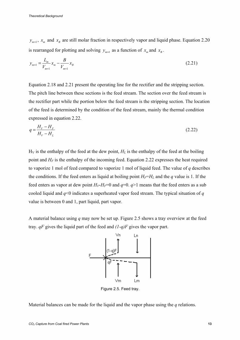
A material balance using q may now be set up. Figure 2.5 shows a tray overview at the feed
tray. qF gives the liquid part of the feed and (1-q)F gives the vapor part.
Figure 2.5. Feed tray.
Material balances can be made for the liquid and the vapor phase using the q relations.
Theoretical Background
CO2 Capture from Coal fired Power Plants 14
m nL L qF= + (2.23)
(1 )n mV V q F= + − (2.24)
Equation 2.14 and 2.20 can be rewritten to 2.25 and 2.26.
n n DV y L x Dx= + (2.25)
m m BV y L x Bx= − (2.26)
Subtracting equation 2.25 from 2.26 gives 2.27.
( ) ( ) ( )m n m n D BV V y L L x Dx Bx− = − − + (2.27)
Rearranging this for y versus x gives equation 2.28.
( ) ( )( ) ( )
m n D B
m n m n
L L Dx Bxy xV V V V
− += −− −
(2.28)
In addition one may include the overall balance D B FDx Bx x+ = and B17 is rewritten to 2.29.
11 1 F
qy x xq q
= −− −
(2.29)
The latest equation is called the q-line equation. This represents the location of the
intersection between the enriching and stripping line. The connection between the equilibrium
line given by equation 2.4, the enriching line given 2.18, the stripping line given by 2.21 and
the q-line given by 2.29, is drawn in figure 2.6.
The equations derived here is the theoretical fundament for air separation. The rest of this
report will focus in a more practical direction in the way of modeling and simulations.
Theoretical Background
CO2 Capture from Coal fired Power Plants 15
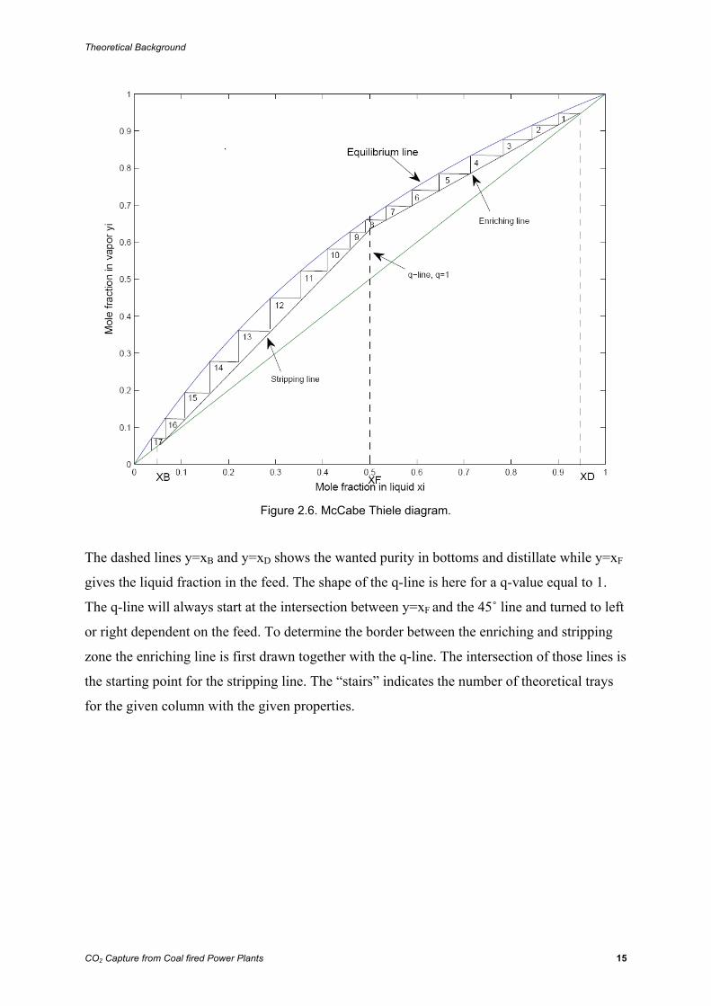
Figure 2.6. McCabe Thiele diagram.
The dashed lines y=xB and y=xD shows the wanted purity in bottoms and distillate while y=xF
gives the liquid fraction in the feed. The shape of the q-line is here for a q-value equal to 1.
The q-line will always start at the intersection between y=xF and the 45˚ line and turned to left
or right dependent on the feed. To determine the border between the enriching and stripping
zone the enriching line is first drawn together with the q-line. The intersection of those lines is
the starting point for the stripping line. The “stairs” indicates the number of theoretical trays
for the given column with the given properties.
Theoretical Background
CO2 Capture from Coal fired Power Plants 16
2.1.2 Air separation unit
2.1.2.1 Introduction
The objective of an air separation unit, ASU, is to convert ambient air to pure oxygen and
pure nitrogen. Normally oxygen is the needed outcome, but in many cases the inert nitrogen
also has a utility value. In air separation for gasification, oxygen is the only utilized product
from the ASU. Although when the gasification is done for power production the nitrogen is
important to dilute the fuel entering the power cycle. In IGCC both oxygen and nitrogen from
the air separation unit is used in the subsequent Gasification Island and Power Island.
An air separation unit may be seen as a cooling machine. Air is compressed, cooled and
choked to remove heat from the cycle. This is done in a temperature area and a pressure level
which leads to liquefied oxygen. The oxygen and nitrogen is separated in a set of distillation
columns. The energy cost of separating oxygen and nitrogen is put on the compression work
of the air compressor. Mature air separation technologies produce oxygen at an energy cost of
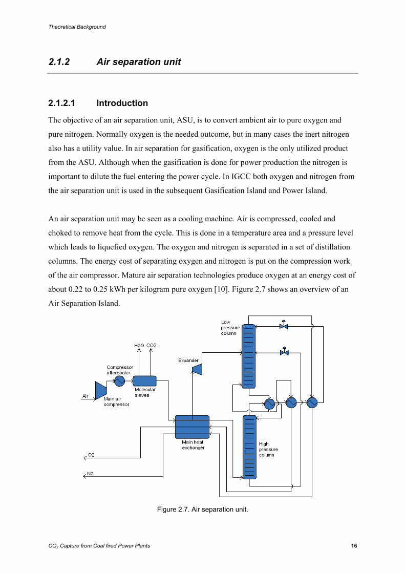
about 0.22 to 0.25 kWh per kilogram pure oxygen [10]. Figure 2.7 shows an overview of an
Air Separation Island.
Figure 2.7. Air separation unit.
Theoretical Background
CO2 Capture from Coal fired Power Plants 17
Figure 2.7 shows a conventional gaseous oxygen (GOX) production plant. When oxygen is
needed at a high pressure it is possible to lower the energy cost with 1-2 percent with a liquid
oxygen (LOX) production plant [7]. The differences between GOX and LOX production are
small and GOX production is first presented before the differences are pointed out in 2.1.2.10
Liquid oxygen.
Ambient air is fed to the main air compressor and compressed to a pressure level at 5-7bar
[10]. The air stream is cooled back to ambient temperature and fed to a molecular sieve for
removal of moisture and carbon dioxide. In the main heat exchanger the air is cooled to a
temperature near dew point before it is fed to the high pressure (HP) column. The column
separates the air into two streams, an almost pure nitrogen stream in the top and an oxygen
rich stream in the bottom. The nitrogen stream is cooled further, chocked to a lower pressure
and fed to the top tray of the low pressure (LP) column. The oxygen stream is choked and fed
about in the middle of the low pressure column. Out of the low pressure column a pure
nitrogen stream is taken out in the top and a pure oxygen stream is taken out in the bottom.
These streams are very cold and are used to cool other parts of the island. Out of the main
heat exchanger the nitrogen and oxygen streams are at ambient temperature and at a pressure
level slightly above atmospheric.
In ASU design, it is important to focus on the outcome of the island. As mentioned, the goal
is to produce pure oxygen and nitrogen. There will always be traces of other substances in a
so called pure gas and one of the main decisions in the design process is to decide the required
purity. It is normal to have oxygen purity between 95 and 99.9 percent dependent on the
subsequent application and the cost of increased purity. For gasification purpose a purity of 95
percent is tolerable [11]. In IGCC nitrogen is diluting the fuel before the power island. To
avoid reaction between oxygen in the nitrogen stream and the fuel before the combustion
chamber a nitrogen purity of 99 percent is demanded [7].
Each of the processes mentioned in the introduction will in the subsequent chapters be closer
explained.
Theoretical Background
CO2 Capture from Coal fired Power Plants 18
2.1.2.2 Compression
At the compressor inlet the air is at ambient conditions. The main air compressor is in real life
a set of several smaller compressors in series. The number of compressors varies with
compression rate and is a question of investment costs versus operating costs. Many
compressors with low lifting height on each compressor give lower operating costs, but larger
investment expenses. On the other hand are fewer compressors with larger lifting heights
cheaper to buy, but demands a larger energy input.
Typical operating pressure for the high pressure column is 5 to 7 bar [11]. The outlet pressure
at the last compressor must be at a level which includes pressure losses in the subsequent
units. This must be done to feed the high pressure column at the wanted pressure.
After compression the air is cooled to a near ambient temperature. The separation island is a
sort of cooling machine and it is advantageous to cool the air as much as possible before the
main heat exchanger. The air cooling after the main compressor is done after each
compression step. The energy demand for compression of cold air is lower than for hot air and
air cooling between each step therefore leads to a lower total energy input.
Cooling of the air gives a 2-3 percent pressure loss in each aftercooler, but decreased energy
consumption for compression of colder air makes it favourable [10].
2.1.2.3 Air cleaning
Before the compressed air enters the main heat exchanger it has to be dried and cleaned. Even
though air mainly consists of nitrogen and oxygen, a small amount of water vapor, argon and
carbon dioxide needs to be taken into account. In addition there are traces of various other
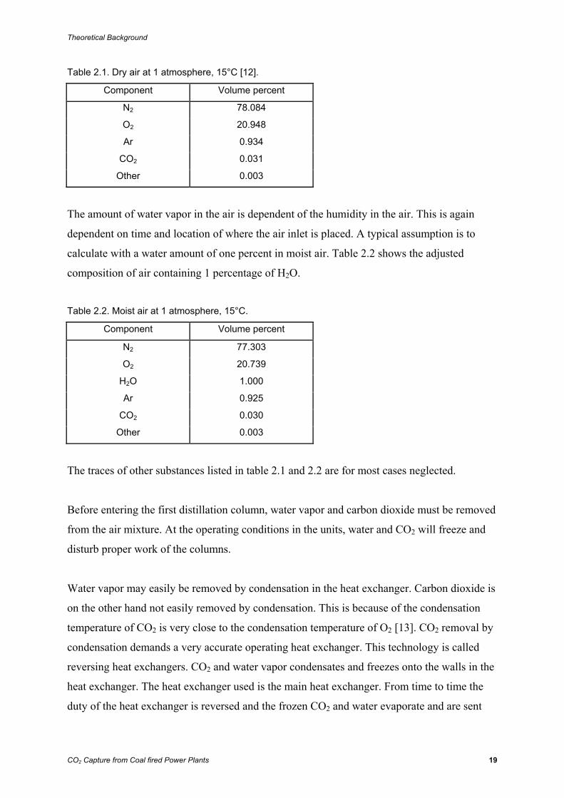
substances, but the amounts of these can be neglected. Table 2.1 gives the composition of 1
atmosphere, 15°C [12].
Theoretical Background
CO2 Capture from Coal fired Power Plants 19
Table 2.1. Dry air at 1 atmosphere, 15°C [12].
Component Volume percent
N2 78.084
O2 20.948
Ar 0.934
CO2 0.031
Other 0.003
The amount of water vapor in the air is dependent of the humidity in the air. This is again
dependent on time and location of where the air inlet is placed. A typical assumption is to
calculate with a water amount of one percent in moist air. Table 2.2 shows the adjusted
composition of air containing 1 percentage of H2O.
Table 2.2. Moist air at 1 atmosphere, 15°C.
Component Volume percent
N2 77.303
O2 20.739
H2O 1.000
Ar 0.925
CO2 0.030
Other 0.003
The traces of other substances listed in table 2.1 and 2.2 are for most cases neglected.
Before entering the first distillation column, water vapor and carbon dioxide must be removed
from the air mixture. At the operating conditions in the units, water and CO2 will freeze and
disturb proper work of the columns.
Water vapor may easily be removed by condensation in the heat exchanger. Carbon dioxide is
on the other hand not easily removed by condensation. This is because of the condensation
temperature of CO2 is very close to the condensation temperature of O2 [13]. CO2 removal by
condensation demands a very accurate operating heat exchanger. This technology is called
reversing heat exchangers. CO2 and water vapor condensates and freezes onto the walls in the
heat exchanger. The heat exchanger used is the main heat exchanger. From time to time the
duty of the heat exchanger is reversed and the frozen CO2 and water evaporate and are sent
Theoretical Background
CO2 Capture from Coal fired Power Plants 20
back to the atmosphere in a waste gas stream. This technology demands a production stop
every time the heat exchanger is cleaned for frozen waste products and is therefore not
optimal for large scale units [14].
The solution for large scale air separators is to use a molecular sieve pre purification unit
(PPU) to remove both water vapor and carbon dioxide. The molecular sieves remove water
vapor and CO2 by adsorption at near ambient conditions. A molecular sieve typically contains
of two vessels where one of the vessels is used to purify the air and the other vessel is being
regenerated. The advantage of molecular sieves is the ability to operate at stationary
conditions with no need for production stop. If the air separation island is located in an
environment with air containing other unwanted components, a molecular sieve can normally
be designed to handle these challenges [14].
After removal of CO2 and water vapor the air is sent to the main heat exchanger.
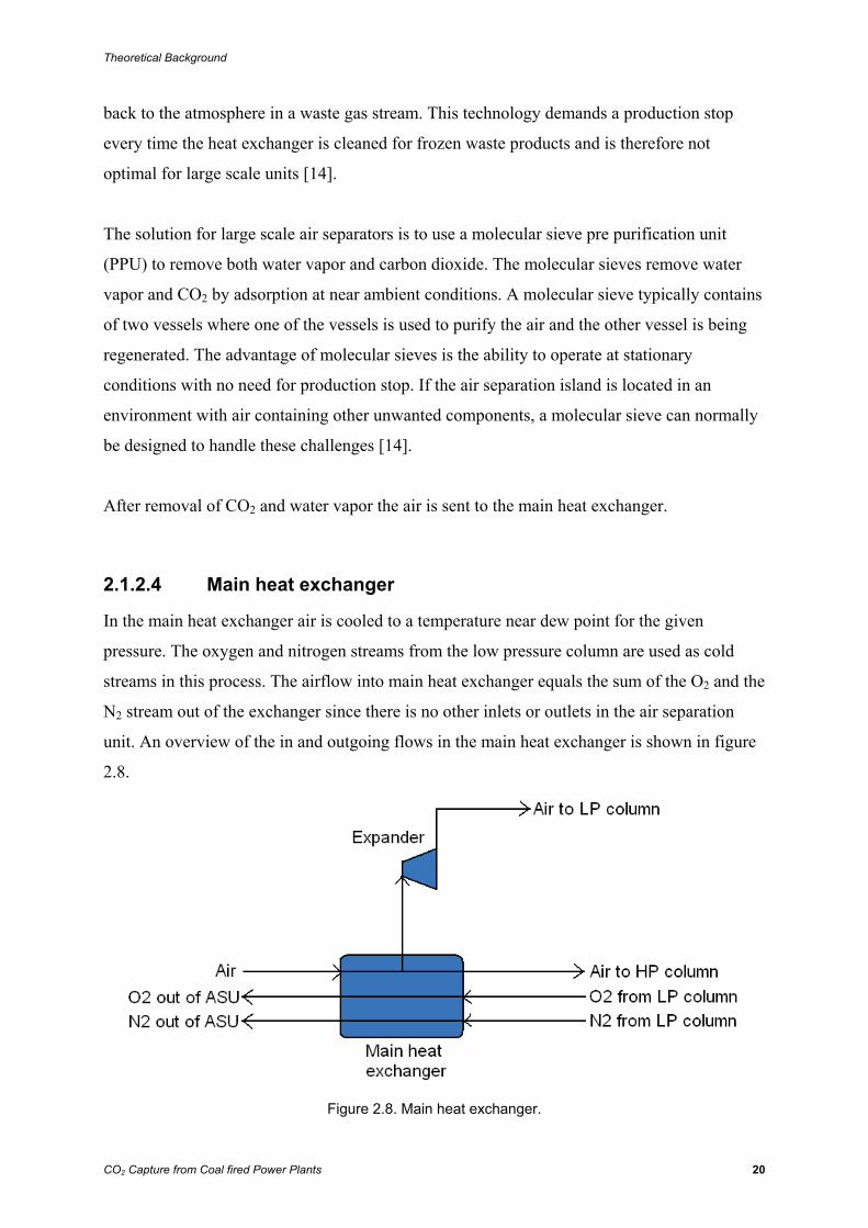
2.1.2.4 Main heat exchanger
In the main heat exchanger air is cooled to a temperature near dew point for the given
pressure. The oxygen and nitrogen streams from the low pressure column are used as cold
streams in this process. The airflow into main heat exchanger equals the sum of the O2 and the
N2 stream out of the exchanger since there is no other inlets or outlets in the air separation
unit. An overview of the in and outgoing flows in the main heat exchanger is shown in figure
2.8.
Figure 2.8. Main heat exchanger.
Theoretical Background
CO2 Capture from Coal fired Power Plants 21
As mentioned in 2.1.2.1 Introduction, an air separation unit may be considered as a cooling
machine. Coldness is produced by compression with aftercooling to near ambient temperature
and choking to achieve temperatures below ambient.
Compression work is the only external energy input to the air separation island. The cold
needed in the unit must be produced by compression, heat exchanging and choking. If there is
an increased demand of coldness, if for example the island is a LOX island instead of a GOX
island, the extra heat removal is produced by a booster compressor with heat exchanging in
the main heat exchanger and choking afterwards. This is closer explained in 2.1.2.10 Liquid
oxygen.
In this heat exchanger a small amount of air is taken out in the exchanger and led to the low
pressure column. This is done to have enough heat in the in the combined condenser and
reboiler between the columns. This is also explained in section 2.1.2.7 Combined condenser
and reboiler. The amount of air sent to the low pressure column is about 10 percent of the
airflow [7].
When designing a heat exchanger an economic consideration about the conduction ability is
required. Heat exchangers with high conduction rates are expensive, but in units with small
temperature differences, like air separators, they are necessary. Due to low temperature
differences in the streams there is no room for low conduction rates. ΔT is the value showing
this minimum temperature difference between hot inlet temperature and cold outlet
temperature, and cold inlet temperature and hot outlet temperature, there can be in a heat
exchanger. ΔT is called minimum temperature approach. A low ΔT gives high conduction
ability, but the heat exchanger is expensive. A high ΔT gives lower conduction ability, but on
the other hand the exchangers are cheaper to buy [15]. As mentioned, air separators normally
have low temperature difference and therefore demands high quality heat exchangers with a
low ΔT. Typical ΔT for exchangers in air separation units are 1-2K [10].
After the main heat exchanger is air at a temperature near dew point for the given pressure
sent to the high pressure column. Pure nitrogen and oxygen are sent out of the air separation
unit to pre treatment.
Theoretical Background
CO2 Capture from Coal fired Power Plants 22
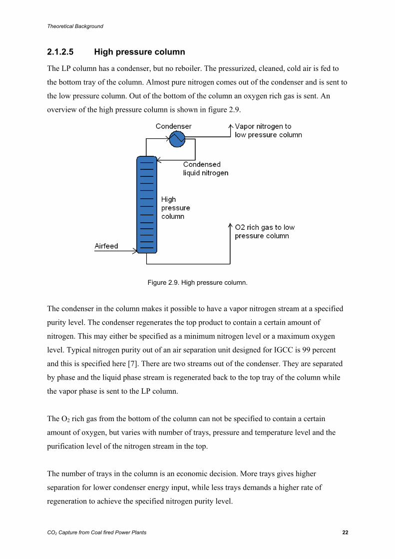
2.1.2.5 High pressure column
The LP column has a condenser, but no reboiler. The pressurized, cleaned, cold air is fed to
the bottom tray of the column. Almost pure nitrogen comes out of the condenser and is sent to
the low pressure column. Out of the bottom of the column an oxygen rich gas is sent. An
overview of the high pressure column is shown in figure 2.9.
Figure 2.9. High pressure column.
The condenser in the column makes it possible to have a vapor nitrogen stream at a specified
purity level. The condenser regenerates the top product to contain a certain amount of
nitrogen. This may either be specified as a minimum nitrogen level or a maximum oxygen
level. Typical nitrogen purity out of an air separation unit designed for IGCC is 99 percent
and this is specified here [7]. There are two streams out of the condenser. They are separated
by phase and the liquid phase stream is regenerated back to the top tray of the column while
the vapor phase is sent to the LP column.
The O2 rich gas from the bottom of the column can not be specified to contain a certain
amount of oxygen, but varies with number of trays, pressure and temperature level and the
purification level of the nitrogen stream in the top.
The number of trays in the column is an economic decision. More trays gives higher
separation for lower condenser energy input, while less trays demands a higher rate of
regeneration to achieve the specified nitrogen purity level.
Theoretical Background
CO2 Capture from Coal fired Power Plants 23
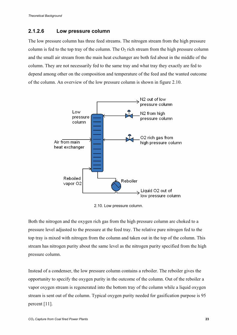
2.1.2.6 Low pressure column
The low pressure column has three feed streams. The nitrogen stream from the high pressure
column is fed to the top tray of the column. The O2 rich stream from the high pressure column
and the small air stream from the main heat exchanger are both fed about in the middle of the
column. They are not necessarily fed to the same tray and what tray they exactly are fed to
depend among other on the composition and temperature of the feed and the wanted outcome
of the column. An overview of the low pressure column is shown in figure 2.10.
2.10. Low pressure column.
Both the nitrogen and the oxygen rich gas from the high pressure column are choked to a
pressure level adjusted to the pressure at the feed tray. The relative pure nitrogen fed to the
top tray is mixed with nitrogen from the column and taken out in the top of the column. This
stream has nitrogen purity about the same level as the nitrogen purity specified from the high
pressure column.
Instead of a condenser, the low pressure column contains a reboiler. The reboiler gives the
opportunity to specify the oxygen purity in the outcome of the column. Out of the reboiler a
vapor oxygen stream is regenerated into the bottom tray of the column while a liquid oxygen
stream is sent out of the column. Typical oxygen purity needed for gasification purpose is 95
percent [11].
Theoretical Background
CO2 Capture from Coal fired Power Plants 24
An analysis on number of trays is done similar to the analysis for the high pressure column.
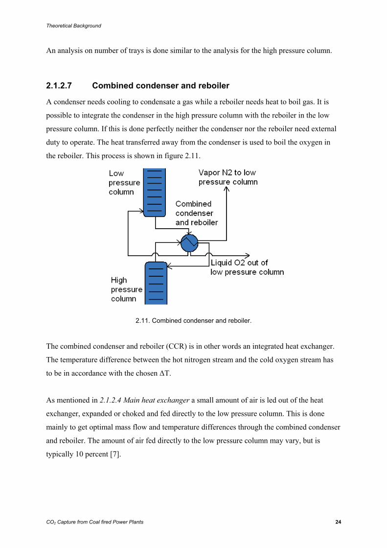
2.1.2.7 Combined condenser and reboiler
A condenser needs cooling to condensate a gas while a reboiler needs heat to boil gas. It is
possible to integrate the condenser in the high pressure column with the reboiler in the low
pressure column. If this is done perfectly neither the condenser nor the reboiler need external
duty to operate. The heat transferred away from the condenser is used to boil the oxygen in
the reboiler. This process is shown in figure 2.11.
2.11. Combined condenser and reboiler.
The combined condenser and reboiler (CCR) is in other words an integrated heat exchanger.
The temperature difference between the hot nitrogen stream and the cold oxygen stream has
to be in accordance with the chosen ΔT.
As mentioned in 2.1.2.4 Main heat exchanger a small amount of air is led out of the heat
exchanger, expanded or choked and fed directly to the low pressure column. This is done
mainly to get optimal mass flow and temperature differences through the combined condenser
and reboiler. The amount of air fed directly to the low pressure column may vary, but is
typically 10 percent [7].
Theoretical Background
CO2 Capture from Coal fired Power Plants 25
2.1.2.8 Subcooler
The nitrogen rich stream between the high pressure and low pressure column needs to be
cooled to a proper temperature level. This level is dependent on many factors as number of
trays in the columns and the duty of the combined condenser and reboiler. To cool the
nitrogen stream, the cold oxygen and nitrogen leaving respectively the bottom and the top of
the low pressure column are utilized. This can be seen in figure 2.7.
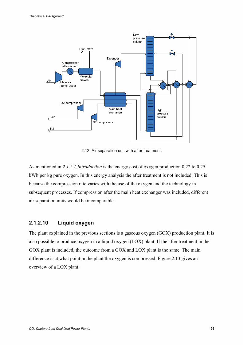
2.1.2.9 After treatment of nitrogen and oxygen
The air separation island described delivers gaseous oxygen and nitrogen at a pressure level
slightly above atmospheric pressure. Typical pressures are 1.5 to 2 bar [11]. The gases are as
mentioned used to cool the incoming air and are therefore heated to about ambient
temperature.
In an IGCC plant both the oxygen and nitrogen are utilized. The oxygen is used in the
gasification process and the nitrogen is used to dilute the H2 rich fuel before the gas turbine.
The gasification pressure is ranging from 20 to 70 bar and even higher for modern gasifiers
[6]. The gas turbine has a pressure level ranging from 10 to 35 depending on technology and
size of the plant [16]. Oxygen and nitrogen both have to be compressed to fulfill their purpose
in the IGCC plant. An overview of a complete air separation island including oxygen and
nitrogen compression is shown in figure 2.12.
Theoretical Background
CO2 Capture from Coal fired Power Plants 26
2.12. Air separation unit with after treatment.
As mentioned in 2.1.2.1 Introduction is the energy cost of oxygen production 0.22 to 0.25
kWh per kg pure oxygen. In this energy analysis the after treatment is not included. This is
because the compression rate varies with the use of the oxygen and the technology in
subsequent processes. If compression after the main heat exchanger was included, different
air separation units would be incomparable.
2.1.2.10 Liquid oxygen
The plant explained in the previous sections is a gaseous oxygen (GOX) production plant. It is
also possible to produce oxygen in a liquid oxygen (LOX) plant. If the after treatment in the
GOX plant is included, the outcome from a GOX and LOX plant is the same. The main
difference is at what point in the plant the oxygen is compressed. Figure 2.13 gives an
overview of a LOX plant.
Theoretical Background
CO2 Capture from Coal fired Power Plants 27
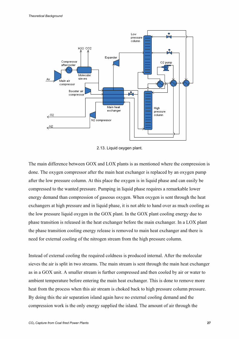
2.13. Liquid oxygen plant.
The main difference between GOX and LOX plants is as mentioned where the compression is
done. The oxygen compressor after the main heat exchanger is replaced by an oxygen pump
after the low pressure column. At this place the oxygen is in liquid phase and can easily be
compressed to the wanted pressure. Pumping in liquid phase requires a remarkable lower
energy demand than compression of gaseous oxygen. When oxygen is sent through the heat
exchangers at high pressure and in liquid phase, it is not able to hand over as much cooling as
the low pressure liquid oxygen in the GOX plant. In the GOX plant cooling energy due to
phase transition is released in the heat exchanger before the main exchanger. In a LOX plant
the phase transition cooling energy release is removed to main heat exchanger and there is
need for external cooling of the nitrogen stream from the high pressure column.
Instead of external cooling the required coldness is produced internal. After the molecular
sieves the air is split in two streams. The main stream is sent through the main heat exchanger
as in a GOX unit. A smaller stream is further compressed and then cooled by air or water to
ambient temperature before entering the main heat exchanger. This is done to remove more
heat from the process when this air stream is choked back to high pressure column pressure.
By doing this the air separation island again have no external cooling demand and the
compression work is the only energy supplied the island. The amount of air through the
Theoretical Background
CO2 Capture from Coal fired Power Plants 28
booster compressor varies with the additional coldness requirement, which again varies with
wanted outcome pressure. The amount is typical 30 percent of the air feed [7].
There is an energy gain from having liquid oxygen pumped to wanted pressure instead of
gaseous oxygen compressed. Almost all the energy gained is lost in the booster air
compressor, but it is possible to reduce the total energy cost with 1 to 2 percent [7]. This
percentage number is dependent on technology and the pressure level the oxygen out of the
island is delivered at. Another advantage with LOX plants is the reduced explosion risk.
There are always some risks when pure oxygen is compressed in gaseous form in a
compressor. The risks are reduced when the pressure rise is done in liquid phase by a pump.
2.1.2.11 Argon treatment
In both the GOX and LOX plants described there is no capture of argon. Argon has its boiling
point very close to oxygen and the separation process is thereby more complex [13]. Including
argon separation demands an extra distillation column and due to the nearby boiling points
between argon and oxygen, the column is a physical large construction. For IGCC purpose the
traces of argon in both the oxygen and nitrogen streams are unimportant.
Argon has no utility value in an IGCC plant, but is used in other processes. It may therefore
be an idea to include argon separation if other industries are willing to buy it. To decide
whether an argon column should be included, an economic analysis concerning the price of
argon compared to the price of an extra column plus the extra energy demand must be
discussed. An air separation island including argon treatment is shown in figure 2.14.
Theoretical Background
CO2 Capture from Coal fired Power Plants 29
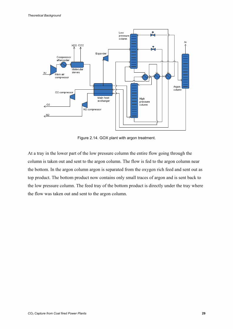
Figure 2.14. GOX plant with argon treatment.
At a tray in the lower part of the low pressure column the entire flow going through the
column is taken out and sent to the argon column. The flow is fed to the argon column near
the bottom. In the argon column argon is separated from the oxygen rich feed and sent out as
top product. The bottom product now contains only small traces of argon and is sent back to
the low pressure column. The feed tray of the bottom product is directly under the tray where
the flow was taken out and sent to the argon column.
Theoretical Background
CO2 Capture from Coal fired Power Plants 30
2.2 Gasification Island
2.2.1 Coal
Coal is the most common source for electricity production all around the world. Coal provides
25% of global primary energy needs and generates 40% of the world's electricity [17].The
consumption of coal is still increasing, especially in China, and it is expected that it will play
a major role as an energy source the next decades. The remaining resources of coal around the
world is proved to be significant larger than for oil and gas. The ratio of reserves to current
production (R/P ratio) is 147, which means that with today's coal consumption the world's
reserves will last 147 years. Corresponding numbers for oil and gas are respectively 40 and 63
[5]. These numbers varies from different sources. Gasification estimates with an R/P ratio for
coal as 216 [6]. Anyhow this demonstrates that coal will be an important part of the energy
market in the upcoming years.
Coal fired power plants are one of the largest source of CO2 world wide. A reduction of coal
consumption in the nearest future seems unrealistic. CO2 capture from coal fired power plants
will probably become one of the main sources to reduce CO2 emissions.
One of the actual technologies of CO2 capture from coal fired power plants is to gasify the
coal and thereafter extract the CO2 before the power cycle. This gasifying process will be
studied closer in the following chapters.
2.2.1.1 Composition
The composition of coal is complex. The resources are distributed all over the world and the
formation process of coal differs and depends on location. Because of the variations in
properties it is hard to make one definition of coal. The varying compositions cause different
properties which affect the performance for instance in a power plant. The main components
in coals are carbon, hydrogen, oxygen, nitrogen and sulfur. The amount of the different
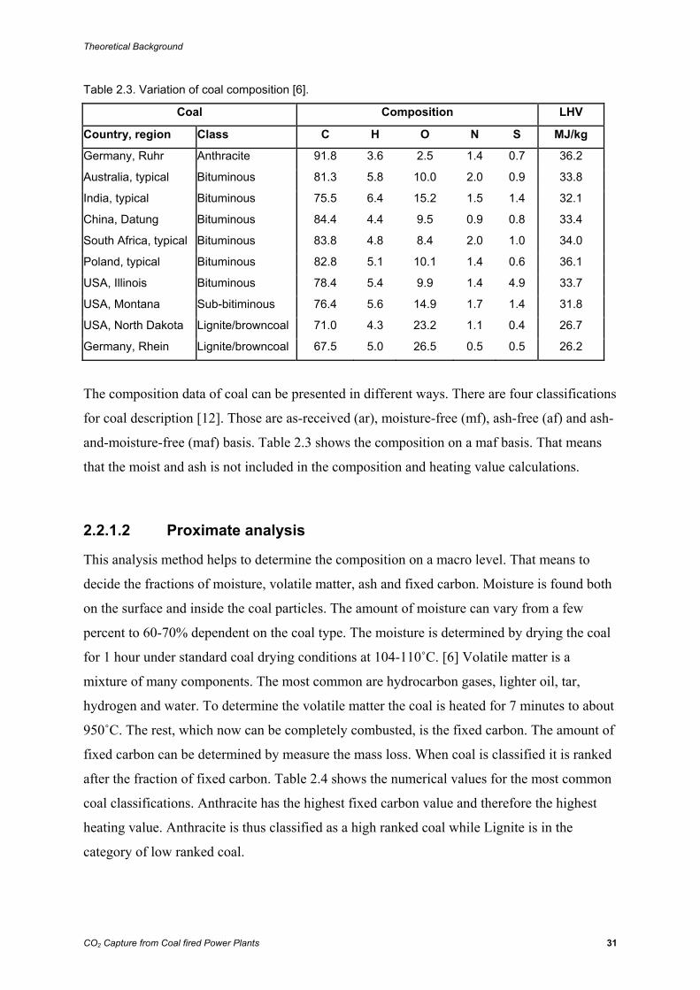
substances decides the heating value of the fuel. Table 2.3 shows the composition and lower
heating value of several types of coal from different regions in the world.
Theoretical Background
CO2 Capture from Coal fired Power Plants 31
Table 2.3. Variation of coal composition [6].
Coal Composition LHV
Country, region Class C H O N S MJ/kg
Germany, Ruhr Anthracite 91.8 3.6 2.5 1.4 0.7 36.2
Australia, typical Bituminous 81.3 5.8 10.0 2.0 0.9 33.8
India, typical Bituminous 75.5 6.4 15.2 1.5 1.4 32.1
China, Datung Bituminous 84.4 4.4 9.5 0.9 0.8 33.4
South Africa, typical Bituminous 83.8 4.8 8.4 2.0 1.0 34.0
Poland, typical Bituminous 82.8 5.1 10.1 1.4 0.6 36.1
USA, Illinois Bituminous 78.4 5.4 9.9 1.4 4.9 33.7
USA, Montana Sub-bitiminous 76.4 5.6 14.9 1.7 1.4 31.8
USA, North Dakota Lignite/browncoal 71.0 4.3 23.2 1.1 0.4 26.7
Germany, Rhein Lignite/browncoal 67.5 5.0 26.5 0.5 0.5 26.2
The composition data of coal can be presented in different ways. There are four classifications
for coal description [12]. Those are as-received (ar), moisture-free (mf), ash-free (af) and ash-
and-moisture-free (maf) basis. Table 2.3 shows the composition on a maf basis. That means
that the moist and ash is not included in the composition and heating value calculations.
2.2.1.2 Proximate analysis
This analysis method helps to determine the composition on a macro level. That means to
decide the fractions of moisture, volatile matter, ash and fixed carbon. Moisture is found both
on the surface and inside the coal particles. The amount of moisture can vary from a few
percent to 60-70% dependent on the coal type. The moisture is determined by drying the coal
for 1 hour under standard coal drying conditions at 104-110˚C. [6] Volatile matter is a
mixture of many components. The most common are hydrocarbon gases, lighter oil, tar,
hydrogen and water. To determine the volatile matter the coal is heated for 7 minutes to about
950˚C. The rest, which now can be completely combusted, is the fixed carbon. The amount of
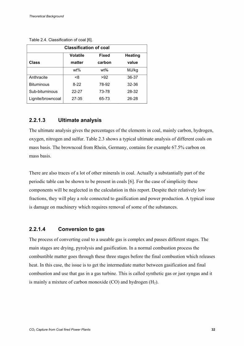
fixed carbon can be determined by measure the mass loss. When coal is classified it is ranked
after the fraction of fixed carbon. Table 2.4 shows the numerical values for the most common
coal classifications. Anthracite has the highest fixed carbon value and therefore the highest
heating value. Anthracite is thus classified as a high ranked coal while Lignite is in the
category of low ranked coal.
Theoretical Background
CO2 Capture from Coal fired Power Plants 32
Table 2.4. Classification of coal [6].
Classification of coal
Class Volatile matter
Fixed carbon
Heating value
wt% wt% MJ/kg
Anthracite <8 >92 36-37
Bituminous 8-22 78-92 32-36
Sub-bituminous 22-27 73-78 28-32
Lignite/browncoal 27-35 65-73 26-28
2.2.1.3 Ultimate analysis
The ultimate analysis gives the percentages of the elements in coal, mainly carbon, hydrogen,
oxygen, nitrogen and sulfur. Table 2.3 shows a typical ultimate analysis of different coals on
mass basis. The browncoal from Rhein, Germany, contains for example 67.5% carbon on
mass basis.
There are also traces of a lot of other minerals in coal. Actually a substantially part of the
periodic table can be shown to be present in coals [6]. For the case of simplicity these
components will be neglected in the calculation in this report. Despite their relatively low
fractions, they will play a role connected to gasification and power production. A typical issue
is damage on machinery which requires removal of some of the substances.
2.2.1.4 Conversion to gas
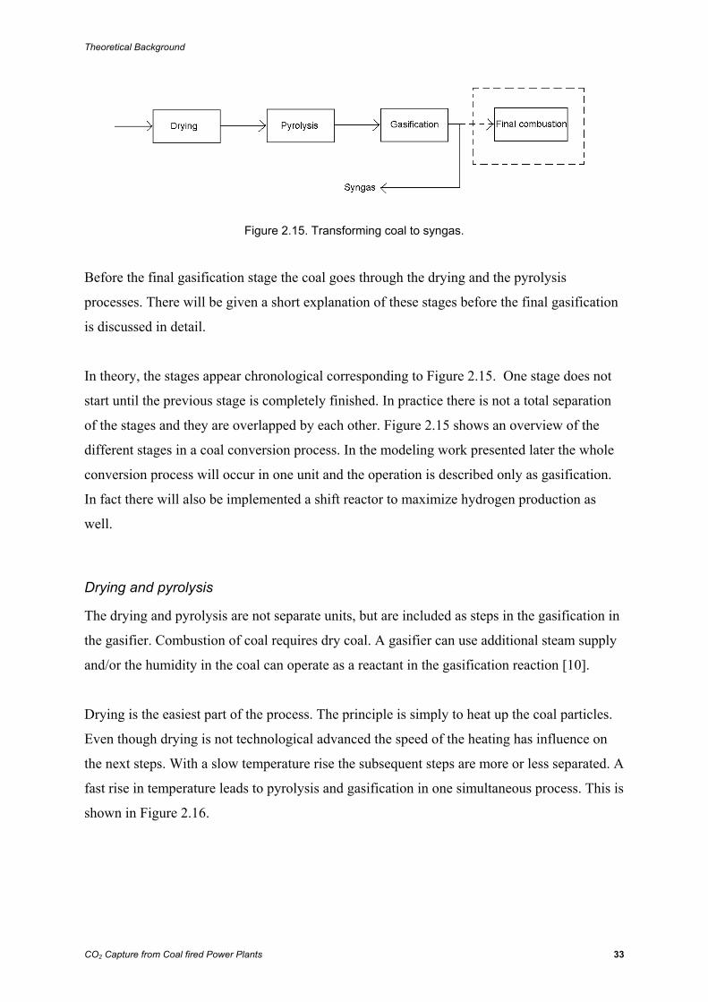
The process of converting coal to a useable gas is complex and passes different stages. The
main stages are drying, pyrolysis and gasification. In a normal combustion process the
combustible matter goes through these three stages before the final combustion which releases
heat. In this case, the issue is to get the intermediate matter between gasification and final
combustion and use that gas in a gas turbine. This is called synthetic gas or just syngas and it
is mainly a mixture of carbon monoxide (CO) and hydrogen (H2).
Theoretical Background
CO2 Capture from Coal fired Power Plants 33
Figure 2.15. Transforming coal to syngas.
Before the final gasification stage the coal goes through the drying and the pyrolysis
processes. There will be given a short explanation of these stages before the final gasification
is discussed in detail.
In theory, the stages appear chronological corresponding to Figure 2.15. One stage does not
start until the previous stage is completely finished. In practice there is not a total separation
of the stages and they are overlapped by each other. Figure 2.15 shows an overview of the
different stages in a coal conversion process. In the modeling work presented later the whole
conversion process will occur in one unit and the operation is described only as gasification.
In fact there will also be implemented a shift reactor to maximize hydrogen production as
well.
Drying and pyrolysis
The drying and pyrolysis are not separate units, but are included as steps in the gasification in
the gasifier. Combustion of coal requires dry coal. A gasifier can use additional steam supply
and/or the humidity in the coal can operate as a reactant in the gasification reaction [10].
Drying is the easiest part of the process. The principle is simply to heat up the coal particles.
Even though drying is not technological advanced the speed of the heating has influence on
the next steps. With a slow temperature rise the subsequent steps are more or less separated. A
fast rise in temperature leads to pyrolysis and gasification in one simultaneous process. This is
shown in Figure 2.16.
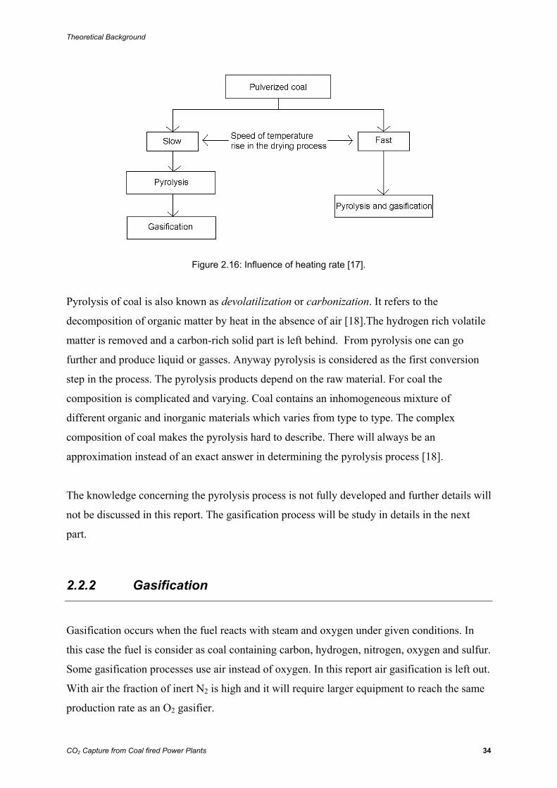
Theoretical Background
CO2 Capture from Coal fired Power Plants 34
Figure 2.16: Influence of heating rate [17].
Pyrolysis of coal is also known as devolatilization or carbonization. It refers to the
decomposition of organic matter by heat in the absence of air [18].The hydrogen rich volatile
matter is removed and a carbon-rich solid part is left behind. From pyrolysis one can go
further and produce liquid or gasses. Anyway pyrolysis is considered as the first conversion
step in the process. The pyrolysis products depend on the raw material. For coal the
composition is complicated and varying. Coal contains an inhomogeneous mixture of
different organic and inorganic materials which varies from type to type. The complex
composition of coal makes the pyrolysis hard to describe. There will always be an
approximation instead of an exact answer in determining the pyrolysis process [18].
The knowledge concerning the pyrolysis process is not fully developed and further details will
not be discussed in this report. The gasification process will be study in details in the next
part.
2.2.2 Gasification
Gasification occurs when the fuel reacts with steam and oxygen under given conditions. In
this case the fuel is consider as coal containing carbon, hydrogen, nitrogen, oxygen and sulfur.
Some gasification processes use air instead of oxygen. In this report air gasification is left out.
With air the fraction of inert N2 is high and it will require larger equipment to reach the same
production rate as an O2 gasifier.
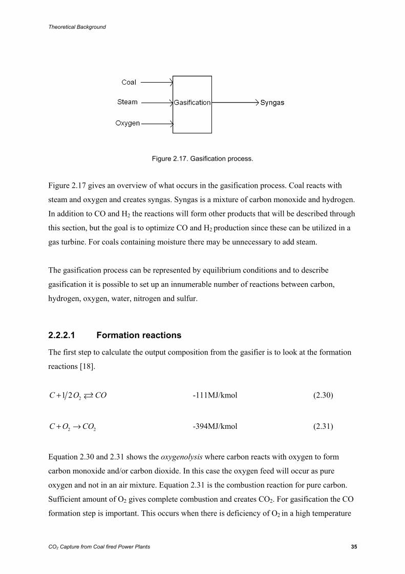
Theoretical Background
CO2 Capture from Coal fired Power Plants 35
Figure 2.17. Gasification process.
Figure 2.17 gives an overview of what occurs in the gasification process. Coal reacts with
steam and oxygen and creates syngas. Syngas is a mixture of carbon monoxide and hydrogen.
In addition to CO and H2 the reactions will form other products that will be described through
this section, but the goal is to optimize CO and H2 production since these can be utilized in a
gas turbine. For coals containing moisture there may be unnecessary to add steam.
The gasification process can be represented by equilibrium conditions and to describe
gasification it is possible to set up an innumerable number of reactions between carbon,
hydrogen, oxygen, water, nitrogen and sulfur.
2.2.2.1 Formation reactions
The first step to calculate the output composition from the gasifier is to look at the formation
reactions [18].
21 2C O CO+ -111MJ/kmol (2.30)
2 2C O CO+ → -394MJ/kmol (2.31)
Equation 2.30 and 2.31 shows the oxygenolysis where carbon reacts with oxygen to form
carbon monoxide and/or carbon dioxide. In this case the oxygen feed will occur as pure
oxygen and not in an air mixture. Equation 2.31 is the combustion reaction for pure carbon.
Sufficient amount of O2 gives complete combustion and creates CO2. For gasification the CO
formation step is important. This occurs when there is deficiency of O2 in a high temperature
Theoretical Background
CO2 Capture from Coal fired Power Plants 36
reactor, above 800˚C [18].The corresponding heat of reaction states if the reactions are
endothermic or exothermic. A negative sign indicates an exothermic reaction meaning that the
reaction will liberate energy, and opposite for a positive sign. The values of the heat of the
reaction are temperature dependent and are here determined for 25˚C (298K). The variation of
the value will though not vary significantly with temperature, as an example the value for
equation 2.30 will increase approximately 5MJ/kmol if the temperature is increased to 1500K.
With deficit of oxygen C may react with CO2 according to the Boudouard reaction [18].
2 2C CO CO+ +172MJ/kmol (2.32)
Methane will also be formed when carbon reacts with hydrogen. This reaction is called
hydrogenolysis. The hydrogen comes from the coal and from the water feed. The later
explained hydrolysis reaction contributes to produce pure H2 [18].
2 42C H CH+ -75MJ/kmol (2.33)
Reaction 2.30 and 2.33 react inverse according to temperature. The production of CO
increases with increasing temperature while the CH4 production is on a maximum level
around 300˚C and decreases with increasing temperature. For power applications with CO2
capture the formation of CO is of interests and reaction 2.30 plays the major role compared to
reaction 2.33. The formation of CO is important because it can react with H2O in a water gas
shift reaction and create H2. This reaction will be discussed in 2.2.2.4 Water gas shift
reaction.
Converting coal to syngas involves water, fed as steam or as a part of the coal. Reaction with
water is called hydrolysis or water gas reaction and it is an endothermic reaction [18].
2 2C H O CO H+ + +131MJ/kmol (2.34)
The water gas reaction also produces more syngas with higher temperature. The partial
pressure of water steam is proportional with syngas production as well.
Theoretical Background
CO2 Capture from Coal fired Power Plants 37
Equation 2.30 and 2.34 describe the most relevant gasification reactions for this case. The
heats of reactions show that reaction 2.30 is exothermic and reaction 2.34 is endothermic.
That indicates that most of the gasification will occur via reaction 2.30. On the other hand
there will be more economical to maximize reaction 2.34. This reaction yields two syngas
molecules per atom of carbon, while the first reaction only gives one syngas molecule.
Another issue is that steam is cheaper than oxygen, so one in this case one will anyway gain
on maximizing the water gas reaction.
Formation of water as a result of hydrogen combustion appears in a well known equation
[18].
2 2 21 2H O H O+ -242MJ/kmol (2.35)
The nitrogen and sulfur will react with the oxygen and form equilibrium with nitric oxide
(NO) and sulfur oxide (SO2) [18].
2 21 2 1 2N O NO+ +90MJ/kmol (2.36)
2 2S O SO+ -362MJ/kmol (2.37)
These substances are represented in small amounts, but they play an important role in the
pollution calculation and they are therefore not neglected.
The sulfur will in a gasification process also react with the hydrogen and create the acid gas
hydrogen sulfide (H2S) [18].
2 2S H H S+ -85MJ/kmol (2.38)
The gasification process occurs as a set of exothermic and endothermic reactions. There will
in a gasification process be an increasing in temperature during the process. This indicates
that some of the chemical energy is transformed to heat. The amount of chemical energy in
the product gas compared to the amount of energy in the feedstock can be expressed as the
cold gas efficiency (CGE).
Theoretical Background
CO2 Capture from Coal fired Power Plants 38
product
feedstock
LHVCGE
LHV= (2.39)
Normal value for CGE is around 0.8 or 80 % [6].
2.2.2.2 Equilibrium equations
The gasification process will roughly appear under equilibrium conditions. Equilibrium states
are helpful for deciding the composition of substances after the gasification. Equation 2.30,
2.31, 2.33, 2.35, 2.36, 2.37 and 2.38 can be rearranged at equilibrium form [18] [19].
[ ]
2
1122
COCO
C O
yK
y y p=⎡ ⎤ ⎡ ⎤⎣ ⎦ ⎣ ⎦
(2.40)
2
2
2
COCO
C O
yK
y y p
⎡ ⎤⎣ ⎦=⎡ ⎤ ⎡ ⎤⎣ ⎦ ⎣ ⎦
(2.41)
2
2
2 2
12
H OH O
H O
yK
y y p
⎡ ⎤⎣ ⎦=⎡ ⎤ ⎡ ⎤⎣ ⎦ ⎣ ⎦
(2.42)
4
4
2
2 2
CHCH
C H
yK
y y p
⎡ ⎤⎣ ⎦=⎡ ⎤ ⎡ ⎤⎣ ⎦ ⎣ ⎦
(2.43)
[ ]
2 2
1 12 2
NONO
O N
yK
y y=⎡ ⎤ ⎡ ⎤⎣ ⎦ ⎣ ⎦
(2.44)
2
2
2
SOSO
S O
yK
y y p
⎡ ⎤⎣ ⎦=⎡ ⎤ ⎡ ⎤⎣ ⎦ ⎣ ⎦
(2.45)
2
2
2
H SH S
S H
yK
y y p
⎡ ⎤⎣ ⎦=⎡ ⎤ ⎡ ⎤⎣ ⎦ ⎣ ⎦
(2.46)
For the equilibrium equations Ki is the equilibrium constant, yi indicates the molar fraction of
the substances and p the pressure. In fact Ki is not constant but temperature dependent. The
values of Ki for a given temperature are tabulated. In a gasification system the temperature
will vary a lot during the process and the equilibrium “constant” has to be modeled as a
function of the temperature.
Theoretical Background
CO2 Capture from Coal fired Power Plants 39
In a reactor producing syngas a lot of reactions occur at the same time. Substances will be
created and broken during the process. Equation 2.30 to 2.38 shows the main reactions in
converting coal, oxygen and steam into synthetic gas. The most interesting component in coal
is the carbon. It is the main energy carrier and its heating value is of interests for the power
production. In fact hydrogen has a higher heating value than carbon on mass basis, but there is
normally significant less amount of it in the coal.
The main product of a gasification process is carbon monoxide and hydrogen. A typical molar
product composition is about 60% CO, 30% H2 and the remaining 10% consist mainly of
CO2, H2O, CH4, NOx, SOx and H2S. The amount of these substances will vary according to
coal type, gasification conditions (temperature and pressure) and the amount of oxygen and
steam in the feed.
The gasification process will be described in more details in 2.2.3 Gasification procedures.
First there will be given short explanation about syngas and the water gas shift reaction.
2.2.2.3 Syngas
Syngas is shorthand for synthesis gas and consist of CO and H2. Other substances in the
product of a gasification process are H2O, CO2 and CH4 etc. The composition is reliant of both
pressure and temperature in the gasifier. For increasing pressure the amount of CO and H2 are
decreasing and the other substances increases correspondingly. For increasing temperature the
amount of CO rise and the amount of H2O, CO2 and CH4 decreases to compensate for the
increase in CO. The H2 quantity is almost constant through temperature oscillations [6].
Syngas is used in a lot of chemical manufacturing processes, for example the production of
ammonia and methanol. In this report the application is focused on power production. Syngas
itself can be utilized in a power cycle using the same principles as a conventional gas turbine.
Syngas can also be converted to a hydrogen rich gas before it enters a power cycle. The
reason for this is to increase the partial pressure of CO2 which makes it easier to remove it. To
manage this, a water gas shift reactor can be installed.
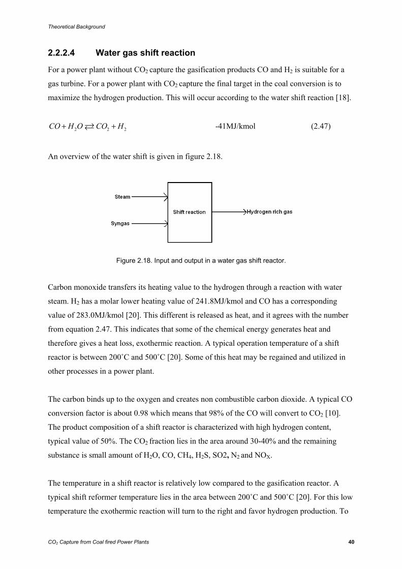
Theoretical Background
CO2 Capture from Coal fired Power Plants 40
2.2.2.4 Water gas shift reaction
For a power plant without CO2 capture the gasification products CO and H2 is suitable for a
gas turbine. For a power plant with CO2 capture the final target in the coal conversion is to
maximize the hydrogen production. This will occur according to the water shift reaction [18].
2 2 2CO H O CO H+ + -41MJ/kmol (2.47)
An overview of the water shift is given in figure 2.18.
Figure 2.18. Input and output in a water gas shift reactor.
Carbon monoxide transfers its heating value to the hydrogen through a reaction with water
steam. H2 has a molar lower heating value of 241.8MJ/kmol and CO has a corresponding
value of 283.0MJ/kmol [20]. This different is released as heat, and it agrees with the number
from equation 2.47. This indicates that some of the chemical energy generates heat and
therefore gives a heat loss, exothermic reaction. A typical operation temperature of a shift
reactor is between 200˚C and 500˚C [20]. Some of this heat may be regained and utilized in
other processes in a power plant.
The carbon binds up to the oxygen and creates non combustible carbon dioxide. A typical CO
conversion factor is about 0.98 which means that 98% of the CO will convert to CO2 [10].
The product composition of a shift reactor is characterized with high hydrogen content,
typical value of 50%. The CO2 fraction lies in the area around 30-40% and the remaining
substance is small amount of H2O, CO, CH4, H2S, SO2, N2 and NOX.
The temperature in a shift reactor is relatively low compared to the gasification reactor. A
typical shift reformer temperature lies in the area between 200˚C and 500˚C [20]. For this low
temperature the exothermic reaction will turn to the right and favor hydrogen production. To

Theoretical Background
CO2 Capture from Coal fired Power Plants 41
maximize the production of H2, the water shift often occurs in two stages with a cooler
between the stages. The temperature from the gasifier can be as high as 1600˚C and a heat
exchanger is required also here to move away heat before the shift reaction [20]. In a
combined cycle this heat can be implemented in the steam cycle to improve efficiency. In a
plant like this were the shift reactor comes after a gasification reactor the pressure will remain
the same in both reactors except the pressure loss.
Particles and acid gases as SO2 and H2S have to be removed before the power cycle. CO2 is
also an acid gas that can be removed together with SO2 and H2S.
2.2.3 Gasification procedures
The gasification process will here be discussed more detailed. This is because the gasification
process has more variables than the water shift. The gasification is very dependent on the
feed, and for coal gasification this is varying for different coal types. The water shift reaction
for H2 production is not varying that much. The products from the gasifier are much the same
since oxygen and steam is regulating the product stream into wanted composition. For power
production this will be about 60% CO and 30% H2 while the last 10% is mainly CO2, N2 H2S
etc [6].
The gasification process occurs as mention as a reaction between the feedstock, oxygen
and/or water steam. It is clear that the amount of the different reactants affect the product. In
addition pressure and temperature also play a role in the gasification. The gasification rate can
be measured as a carbon conversion rate. That means the fraction of carbon that is gasified to
the fraction of carbon in the feedstock [6].
[ ][ ]
productconversion
feedstock
C kmolC
C kmol= (2.48)
The conversion rate lies closed to 1 (100%) for modern gasification reactors.
One can assume the coal feed as a given composition. There will off course appear different
coal types in a gasifier, but for each coal type a modeling/calculation can be done. The coal
feed is given and the gasification process is regulated by the amount of feed, steam and
Theoretical Background
CO2 Capture from Coal fired Power Plants 42
oxygen. 1mol of coal will normally consume from 0.2 to 0.5mol oxygen. The amount of
steam and oxygen regulates the temperature and the wanted composition. The general rule is
that CO production is favored with stoichiometric deficiency of O2 at high temperature
(1500˚C). It is obvious that the hydrogen production will increase with increasing steam rates,
but it is a limit how much of the water that is converted. For optimization the H2 production
rate, the mentioned shift reactor is installed.
Temperature plays a major role in gasification when it directly affects the composition of the
product. At low temperatures production of methane is favored, while higher temperature
increases the syngas (CO + H2) production. Modern gasifiers, which are designed for syngas
production, operate at temperature levels up to 1500˚C and even higher [6]. Increasing the
amount of O2 in the gasifier increases the temperature while injection of water steam works
opposite.
The pressure will not affect the compositions considerably. There are however advantages to
gasify under pressure regarding to equipment size and compression energy. Modern processes
are operated at pressures from 10bar and up to 100bar [6]. For an IGCC application the
normal operating pressure lays in the area between 15bar and 40bar [16]. When CO2 capture
is implemented a high pressure is required to ease the capture procedure [10].
There are different gasification reactors. The reactor type strongly influence the temperature
distribution, and in this way the product composition [18]. The main gasification procedures
are moving-bed gasifiers, fluid-bed gasifiers and entrained flow gasifiers. The last one is most
relevant for IGCC applications. In the upcoming chapters the moving-bed and the fluidized
bed methods will be discussed briefly, before the entrained flow gasification system will be
discussed closer.
2.2.3.1 Moving-bed gasifiers
Moving-bed is the oldest gasification process and it played an important role of producing
syngas from coal in the early stages of gasification. This technology is often called fixed-bed
gasifier. The principle of this process is that the gravity drags the feedstock (here coal) slowly
downwards and the gasification occur when a counter-current blast reacts with the coal. The
gasification products (syngas) flow upwards and preheat the down flowing coal. An overview

Theoretical Background
CO2 Capture from Coal fired Power Plants 43
of this process is given in figure 2.19. Moving-bed process is characterized with low oxygen
consumption and a relatively low outlet temperature. A negative factor of this process is that
the low temperature and the low oxygen consumption affect the gasification rate. Not all of
the feed is gasified and there are pyrolysis products presented in the syngas. Moving-bed
gasifiers have moving parts like for example a stirrer. These equipments required a relatively
high amount of maintenance [6].
Figure 2.19. Lurgi Dry Ash Gasifier.
A very common moving-bed patent is the Lurgi Dry Ash Gasifier. The principles here are the
same as for a general moving-bed facility. The Lurgi process is however using pure O2 in the
gasification process instead of air and it operates under higher pressure than atmospheric.
Pulverized coal is fed from the top via a lock hopper. The lock hopper technology will be
discussed closer in chapter 2.2.3.5 Feeding procedures for a gasifier. The coal is spread in the
reactor by a mechanical distribution device and moves slowly downwards undergoing the
gasification process reacting with O2 and water steam. The Lurgi reactor vessel is a double-
walled room where the space between the walls is filled with boiling water. This is used as
cooling as well as reactant in the gasification process [6].
The composition of the product gas from a Lurgi gasifier depends on the composition of the
feedstock. For coal gasification this means the ranking of the coal according to carbon
content, hydrogen content etc. A rough estimate of the product gases from this type of a
gasifier gives around 30% CO2, 20% CO and 40% H2 on molar basis. The last 10% is a
Theoretical Background
CO2 Capture from Coal fired Power Plants 44
mixture of CH4, N2 and other trace elements. These numbers varies though according to coal
type, but it gives a useable overview. Carbon conversion rate can be as high as 99% [6].
Lurgi gasifiers are spread all over the world. The SASOL complex in South Africa is the
largest gasification plant in the world according to Higmans Gasification edition from 2003.
This plant uses Lurgi dry ash gasifiers and produces 55million Nm3 per day.
Other commercial Moving-bed gasifiers are British Gas/Lurgi (BGL) Slagging Gasifier and
the Ruhr 100 gasifier. The BGL is an improvement of the Lurgi gasifiers designed for
slagging conditions. This gives an increasing in CO production and a reduction in the steam
consumption. The Ruhr 100 gasifier is a version of the Lurgi gasifier constructed to handle
high pressure, 100 bar[6].
2.2.3.2 Fluid-bed gasifiers
Fluidized bed gasifiers are fed with pulverized coal and this is lifted by feed and product
gasses. Steam/oxygen is fed near bottom and mixes with the pulverized coal and reacts while
the fluidized state is kept.
This technology gives a good mixing between feed and oxygen/air and steam. It operates at
relatively low temperature as low as 800˚C for biomass and 950˚C for coal. For coal
gasification the carbon conversion rate is low. The best of existing facilities have a rate up to
97%. Low ranked coal and biomass are more suitable for a fluid-bed gasifier. These are
reactive feedstock which not requires too high temperature and the conversion rate may then
exceed 99%. Problem with fluidizing coal is the case that coal differs so much in shape and
composition. The particles should not be larger than 10 mm. However too small particles will
entrain in the syngas and not get satisfactory gasified. A more detailed description will not be
given here because for the purpose of IGCC plants, this technology is not relevant [6] [18].
2.2.3.3 Entrained-flow gasifiers
Entrained-flow gasifiers are the most common for using in IGCC plants. It operates under
high temperature and requires considerable amounts of oxygen. The gasifier is very flexible
according to feedstock and all coal types can be fed. However, coals with high moisture will
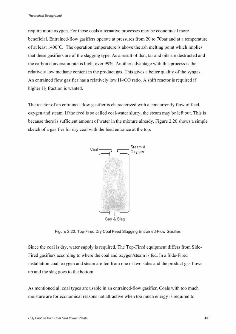
Theoretical Background
CO2 Capture from Coal fired Power Plants 45
require more oxygen. For those coals alternative processes may be economical more
beneficial. Entrained-flow gasifiers operate at pressures from 20 to 70bar and at a temperature
of at least 1400˚C. The operation temperature is above the ash melting point which implies
that these gasifiers are of the slagging type. As a result of that, tar and oils are destructed and
the carbon conversion rate is high, over 99%. Another advantage with this process is the
relatively low methane content in the product gas. This gives a better quality of the syngas.
An entrained flow gasifier has a relatively low H2/CO ratio. A shift reactor is required if
higher H2 fraction is wanted.
The reactor of an entrained-flow gasifier is characterized with a concurrently flow of feed,
oxygen and steam. If the feed is so called coal-water slurry, the steam may be left out. This is
because there is sufficient amount of water in the mixture already. Figure 2.20 shows a simple
sketch of a gasifier for dry coal with the feed entrance at the top.
Figure 2.20. Top-Fired Dry Coal Feed Slagging Entrained-Flow Gasifier.
Since the coal is dry, water supply is required. The Top-Fired equipment differs from Side-
Fired gasifiers according to where the coal and oxygen/steam is fed. In a Side-Fired
installation coal, oxygen and steam are fed from one or two sides and the product gas flows
up and the slag goes to the bottom.
As mentioned all coal types are usable in an entrained-flow gasifier. Coals with too much
moisture are for economical reasons not attractive when too much energy is required to
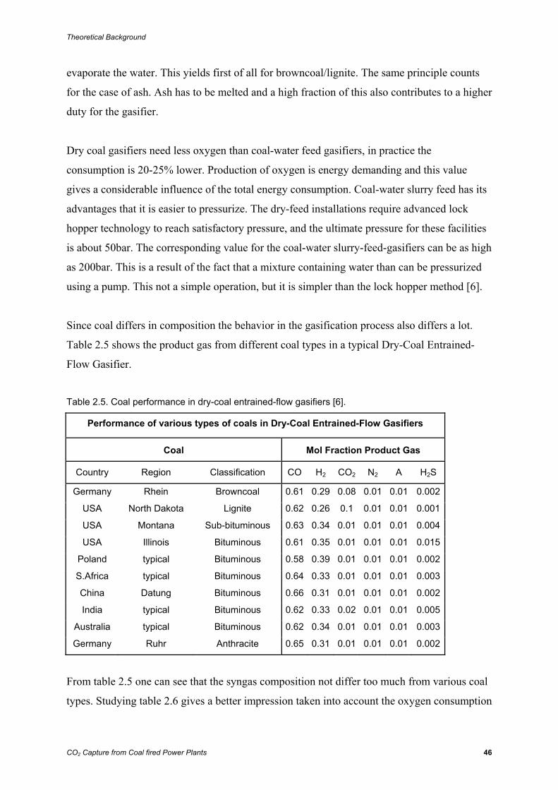
Theoretical Background
CO2 Capture from Coal fired Power Plants 46
evaporate the water. This yields first of all for browncoal/lignite. The same principle counts
for the case of ash. Ash has to be melted and a high fraction of this also contributes to a higher
duty for the gasifier.
Dry coal gasifiers need less oxygen than coal-water feed gasifiers, in practice the
consumption is 20-25% lower. Production of oxygen is energy demanding and this value
gives a considerable influence of the total energy consumption. Coal-water slurry feed has its
advantages that it is easier to pressurize. The dry-feed installations require advanced lock
hopper technology to reach satisfactory pressure, and the ultimate pressure for these facilities
is about 50bar. The corresponding value for the coal-water slurry-feed-gasifiers can be as high
as 200bar. This is a result of the fact that a mixture containing water than can be pressurized
using a pump. This not a simple operation, but it is simpler than the lock hopper method [6].
Since coal differs in composition the behavior in the gasification process also differs a lot.
Table 2.5 shows the product gas from different coal types in a typical Dry-Coal Entrained-
Flow Gasifier.
Table 2.5. Coal performance in dry-coal entrained-flow gasifiers [6].
Performance of various types of coals in Dry-Coal Entrained-Flow Gasifiers
Coal Mol Fraction Product Gas
Country Region Classification CO H2 CO2 N2 A H2S
Germany Rhein Browncoal 0.61 0.29 0.08 0.01 0.01 0.002
USA North Dakota Lignite 0.62 0.26 0.1 0.01 0.01 0.001
USA Montana Sub-bituminous 0.63 0.34 0.01 0.01 0.01 0.004
USA Illinois Bituminous 0.61 0.35 0.01 0.01 0.01 0.015
Poland typical Bituminous 0.58 0.39 0.01 0.01 0.01 0.002
S.Africa typical Bituminous 0.64 0.33 0.01 0.01 0.01 0.003
China Datung Bituminous 0.66 0.31 0.01 0.01 0.01 0.002
India typical Bituminous 0.62 0.33 0.02 0.01 0.01 0.005
Australia typical Bituminous 0.62 0.34 0.01 0.01 0.01 0.003
Germany Ruhr Anthracite 0.65 0.31 0.01 0.01 0.01 0.002
From table 2.5 one can see that the syngas composition not differ too much from various coal
types. Studying table 2.6 gives a better impression taken into account the oxygen consumption
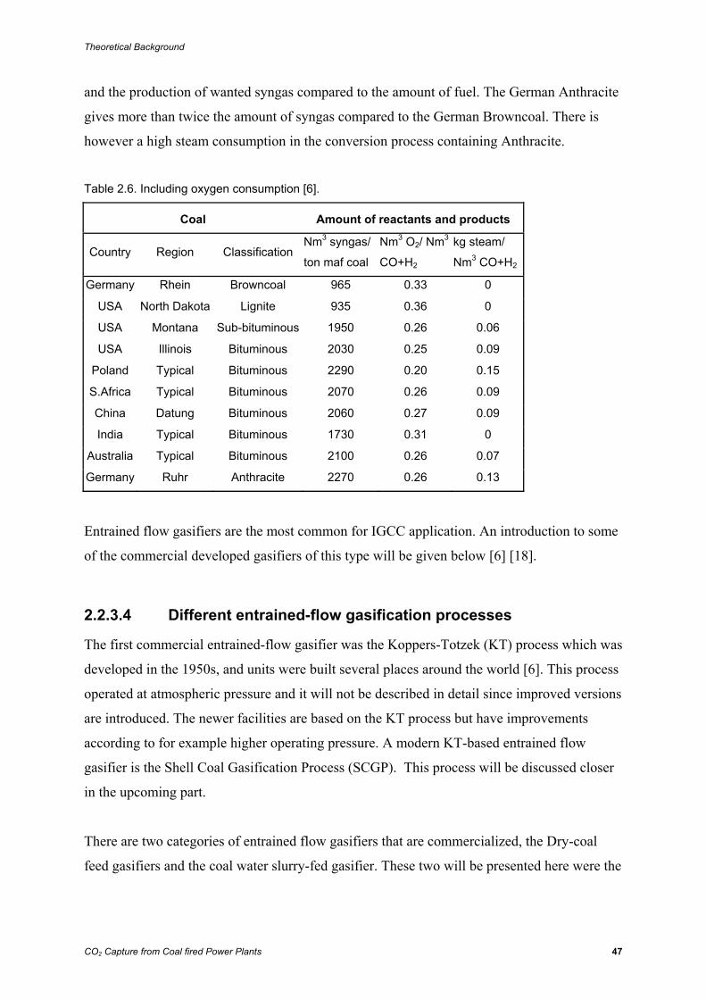
Theoretical Background
CO2 Capture from Coal fired Power Plants 47
and the production of wanted syngas compared to the amount of fuel. The German Anthracite
gives more than twice the amount of syngas compared to the German Browncoal. There is
however a high steam consumption in the conversion process containing Anthracite.
Table 2.6. Including oxygen consumption [6].
Coal Amount of reactants and products
Country Region Classification Nm3 syngas/
ton maf coal
Nm3 O2/ Nm3
CO+H2
kg steam/
Nm3 CO+H2
Germany Rhein Browncoal 965 0.33 0
USA North Dakota Lignite 935 0.36 0
USA Montana Sub-bituminous 1950 0.26 0.06
USA Illinois Bituminous 2030 0.25 0.09
Poland Typical Bituminous 2290 0.20 0.15
S.Africa Typical Bituminous 2070 0.26 0.09
China Datung Bituminous 2060 0.27 0.09
India Typical Bituminous 1730 0.31 0
Australia Typical Bituminous 2100 0.26 0.07
Germany Ruhr Anthracite 2270 0.26 0.13
Entrained flow gasifiers are the most common for IGCC application. An introduction to some
of the commercial developed gasifiers of this type will be given below [6] [18].
2.2.3.4 Different entrained-flow gasification processes
The first commercial entrained-flow gasifier was the Koppers-Totzek (KT) process which was
developed in the 1950s, and units were built several places around the world [6]. This process
operated at atmospheric pressure and it will not be described in detail since improved versions
are introduced. The newer facilities are based on the KT process but have improvements
according to for example higher operating pressure. A modern KT-based entrained flow
gasifier is the Shell Coal Gasification Process (SCGP). This process will be discussed closer
in the upcoming part.
There are two categories of entrained flow gasifiers that are commercialized, the Dry-coal
feed gasifiers and the coal water slurry-fed gasifier. These two will be presented here were the
Theoretical Background
CO2 Capture from Coal fired Power Plants 48
SCGP represents the dry-fed and the Texaco process represents the slurry fed. Some other
processes will also be discussed.
Shell Coal Gasification Process (SCGP)
This is a pressurized version of KT and was developed as a co-operation between Kopper and
Shell. Two commercial plants are built so far as parts in ICGG plants. These have a
production capacity of 2000 and 3000 tons per day. Shell has in addition several ongoing
projects in China.
The SGCP is an up flowing gasifier meaning that the product gas leaves the reactor at the top.
It is a dry-coal process so the feed has to be pressurized using a lock hopper. The coal is sized
below 90μm and mixed with a transportation gas, normally nitrogen. The pressurized coal is
than fed at typical four burners at the side walls where it reacts with oxygen. The reactions are
fast (0.5-4 seconds) and bring along an up flowing syngas and a down flowing slag. The
gasification temperature is about 1500˚C and the pressure is 30-40bar. The product
composition is typically two thirds CO, and one third H2. There will also here be other
substances as CO2, CH4 etc, but the production of CO and H2 is maximized. An almost similar
process is the so called Prenflo process. The SCGP and the Prenflo is often mentioned in the
same descriptions [6].
The Texaco Process
The Texaco process was developed in the late 1940s mainly focused on natural gas. In the
1970s Texaco developed the technology to focus on coal gasification. Several plants for
production of ammonia, methanol and town gas are placed in Japan, China and USA. The
technology is also used in some IGCC units for instance the Polk Power Station in Florida [6].
The Texaco process is a slurry-feed gasifier were moist coal and oxygen enters at the top of
the reactor. It is a down flowing entrained reactor were syngas and slag leave at the bottom.
The feedstock is sized to about 100μm, slurried and pressurized with using a pump. The
reactor pressure varies depending of it is a chemical plant or an IGCC facility. The slurry feed
makes it possible to reach high pressure and for chemical application the pressure may be up
to 80bar. For IGCC plants a typical operation pressure is about 40bar. The temperature is
typically 1500˚C [6].
Theoretical Background
CO2 Capture from Coal fired Power Plants 49
The Texaco gasifier is the most inexpensive design on the market [6]. It is however very
maintenance-intensive and to maximize production an extra standby reactor may be
necessary. This will make the plant more expensive, so an economical calculation must be
done to determine if it is a good investment all in all.
Recently the Texaco gasifier is better known as the GE gasifier when GE bought the
gasification technology from Texaco.
Other gasifying processes
There are some other gasifying processes in the market, both older technology and brand new
ones under construction. The Noell Process was developed by Deutsches Brennstoffinstitut
Freiberg in 1975 and is better known under the name GSP. This is a dry-feed down flowing
system with different variations of reactor design for different feedstocks.
The E-Gas Process is a two stage gasifier with coal-slurry feed. This gasifier handles low
ranked coal and operating temperature at the first stage is 1400˚C. There are built a couple of
IGCC plants in the USA using this technology [6].
There are two modern gasification processes recently developed in Japan for IGCC
application. This is a gasifier constructed by Clean Coal Power R&D Company (CCP) and the
gasifier is named the CCP Gasifier. The CCP combines the pressurized dry-feed technology
with a two stage feeding using air as oxidant. In other word a combination of the SCGP and
the E-Gas processes. The outlet temperature is about 1000˚C and the carbon conversion rate is
closed to 100%. The other gasifier is under construction and is called the Eagle gasifier. This
is a two stage gasifier using oxygen as oxidant and it has a high operation temperature at the
first stage, 1600˚C [6].
Shell and the Texaco (GE) have most commercial experience on gasifiers, and these two
processes are the most common around the world. They represent the two feeding processes
and are therefore well usable examples of entrained flow gasifiers. The two processes have
their advantages and disadvantages. The slurry fed Texaco gasifier can operate on very high
pressure and the pressurizing system is simpler to handle than the Lock hopes system used in
the Shell gasifier. In the other end it needs more oxygen. That both increases the energy
consumption regarding to oxygen production and reduces the cold gas efficiency. The Shell

Theoretical Background
CO2 Capture from Coal fired Power Plants 50
system requires less oxygen per produced amount of syngas but it can not operate on much
higher pressure than 40bar. For IGCC applications this pressure is high enough. In addition is
the oxygen consumption a considerably part of the total energy balance, so a minimum
consumption is preferred. A high pressure is however profitably when it comes to CO2
removal. About 40bar is anyway high since the molar fraction of CO2 is over 0.3 after the
gasification and shift reactor [6].
2.2.3.5 Feeding procedures for a gasifier
The gasification process operates at different pressure depending on the application area
downstream the gasifier. For power production the gasification pressure normally lays in the
range 20 to 40 bar [6]. A challenge for this kind of process is to feed the coal into an area with
that pressure level. The problem occurs because of the fact that coal is a solid matter.
Different techniques are developed to manage this duty. There are two approaches for
pressurizing coal, Dry-Coal Feeding with Lock Hoppers and Pumping Coal as a Coal-Water
Slurry [6]. The feed in a Dry-Coal gasifier is considered as dry, but in practice it will contain
some humidity. This is not a problem for the gasification process since water anyway is a part
of the gasification reaction
The Lock Hopper method is in short a three vessel system where each vessel operates at
different pressure. They are connected to each other with valves and can be seen as a sluicing
system. The solid matter is fed together with an inert gas from top at atmospheric pressure.
The valve between the top hopper and the middle one (the lock hopper) is than open while the
valve between the middle one and the bottom one is closed. After the lock hopper has been
filled the upper valve is closed and the valve at the bottom is open. The pressure at the bottom
hopper is high and the opening of the valve results in a pressure rise in the lock hopper.
In the Lock Hopper feeding method pulverized coal is fed with a transport gas often presented
as nitrogen, syngas or carbon dioxide. For IGCC application nitrogen is the most common
transport gas. Nitrogen is available from the air separation unit (ASU) and it will not affect
the overall gasification efficiency considerable. The use of transport gasses makes it less
attractive to rise the pressure in the gasification process when that results in a higher
consumption of the given transport gas. Normally a dry-coal feed gasifier will not run at
Theoretical Background
CO2 Capture from Coal fired Power Plants 51
higher pressure than 40 bar. This will not affect the case of IGCC while the pressure here
normally is about 20 bar [6].
Pumping Coal as a Coal-Water Slurry is another method for pressurization coal. Slurry of coal
and water is pressurized using a pump. This has its advantage on higher pressure rate and less
advanced equipment than the Dry Feed Gasifyer. A slurry pump can deliver an outlet pressure
as high as 200bar. This increases the capacity and higher pressure is also beneficial regarding
to the CO2 removal downstream the gasifier [20]. The disadvantages using this feeding
technology is that it requires more oxygen since vaporization of water needs more heat.
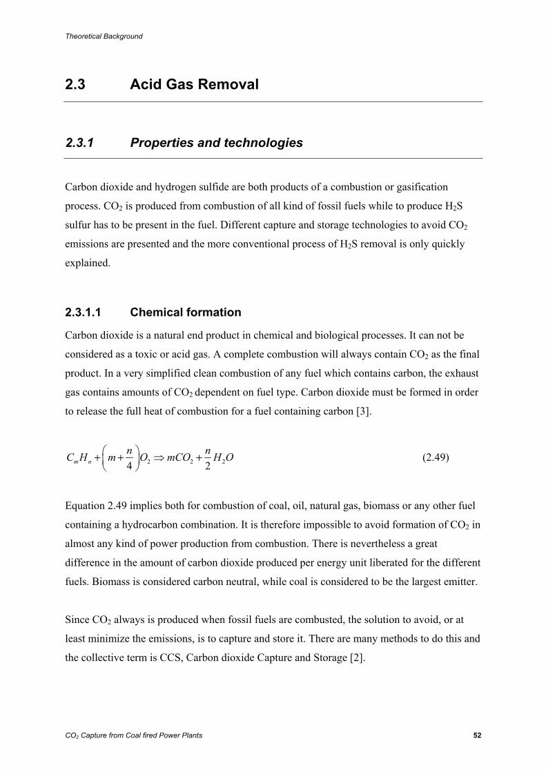
Theoretical Background
CO2 Capture from Coal fired Power Plants 52
2.3 Acid Gas Removal
2.3.1 Properties and technologies
Carbon dioxide and hydrogen sulfide are both products of a combustion or gasification
process. CO2 is produced from combustion of all kind of fossil fuels while to produce H2S
sulfur has to be present in the fuel. Different capture and storage technologies to avoid CO2
emissions are presented and the more conventional process of H2S removal is only quickly
explained.
2.3.1.1 Chemical formation
Carbon dioxide is a natural end product in chemical and biological processes. It can not be
considered as a toxic or acid gas. A complete combustion will always contain CO2 as the final
product. In a very simplified clean combustion of any fuel which contains carbon, the exhaust
gas contains amounts of CO2 dependent on fuel type. Carbon dioxide must be formed in order
to release the full heat of combustion for a fuel containing carbon [3].
2 2 24 2m nn nC H m O mCO H O⎛ ⎞+ + ⇒ +⎜ ⎟
⎝ ⎠ (2.49)
Equation 2.49 implies both for combustion of coal, oil, natural gas, biomass or any other fuel
containing a hydrocarbon combination. It is therefore impossible to avoid formation of CO2 in
almost any kind of power production from combustion. There is nevertheless a great
difference in the amount of carbon dioxide produced per energy unit liberated for the different
fuels. Biomass is considered carbon neutral, while coal is considered to be the largest emitter.
Since CO2 always is produced when fossil fuels are combusted, the solution to avoid, or at
least minimize the emissions, is to capture and store it. There are many methods to do this and
the collective term is CCS, Carbon dioxide Capture and Storage [2].
Theoretical Background
CO2 Capture from Coal fired Power Plants 53
2.3.1.2 Combustion and capture methods
There are many technologies for both capture and storage of carbon dioxide. The technologies
vary from research phase and demonstration plants to well-developed technologies.
Main capture technologies according to power production are post-combustion-, pre-
combustion- and oxyfuel combustion capture [2]. In post-combustion CO2 capture the carbon
dioxide is captured from the exhaust gas after the combustion. The drawback of this
technology is the relative low CO2 concentration in the exhaust gas due to nitrogen in the air.
Pre-combustion capture is CO2 capture before the combustion. This is the method utilized in
IGCC where fuel is transformed into a gas containing mainly H2 and CO2. The carbon dioxide
is separated from the hydrogen before the hydrogen is sent to the combustion chamber.
Oxyfuel combustion is combustion with pure oxygen instead of air. The exhaust gas from
oxyfuel-combustion contains mainly water and CO2 and the substances are easily separated
by condensing the water. The drawback is the cost of producing pure oxygen and the fact that
combustion with pure oxygen requires new types of turbines and technology.
A common drawback for all the capture technologies is the extra energy consumption
required. As a rule of thumb, a power plant with CO2 capture consumes about 15 to 30
percent more fuel to produce the same amount of electricity and heat as an equal plant without
capture facilities. This equals a reduction of 7 to 15 percent points in efficiency [16] [21].
The most explored and most likely to be the common storage technology in the future is
geological storage. This may be done by storage in empty gas or oil fields or in saline
formations. It is also possible to use CO2 to increase the pressure in oil fields by Enhanced Oil
Recovery (EOR). In addition to store carbon dioxide this technology increases the production
from a well. Another technology with a large potential in the future is deep sea storage. The
ocean is capable to receive great amounts of carbon dioxide and keep it there [2].
As mentioned above, IGCC with CO2 capture utilizes pre-combustion capture technology. It
is of cause possible to use post-combustion technology in an IGCC plant, but this gives a
remarkable energy efficiency reduction. In the subsequent part the different methods to
separate the hydrogen and carbon dioxide is looked further into. The issue of storage is
independent of capture technology and storage location is not further discussed in this report.
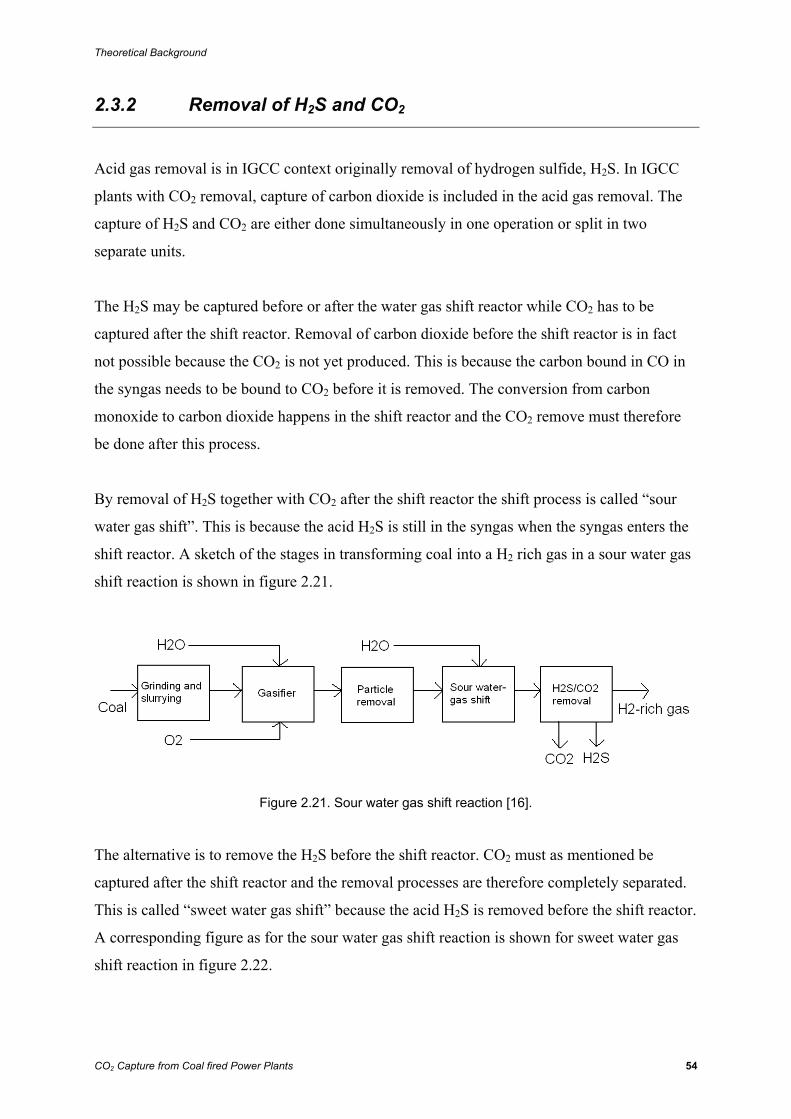
Theoretical Background
CO2 Capture from Coal fired Power Plants 54
2.3.2 Removal of H2S and CO2
Acid gas removal is in IGCC context originally removal of hydrogen sulfide, H2S. In IGCC
plants with CO2 removal, capture of carbon dioxide is included in the acid gas removal. The
capture of H2S and CO2 are either done simultaneously in one operation or split in two
separate units.
The H2S may be captured before or after the water gas shift reactor while CO2 has to be
captured after the shift reactor. Removal of carbon dioxide before the shift reactor is in fact
not possible because the CO2 is not yet produced. This is because the carbon bound in CO in
the syngas needs to be bound to CO2 before it is removed. The conversion from carbon
monoxide to carbon dioxide happens in the shift reactor and the CO2 remove must therefore
be done after this process.
By removal of H2S together with CO2 after the shift reactor the shift process is called “sour
water gas shift”. This is because the acid H2S is still in the syngas when the syngas enters the
shift reactor. A sketch of the stages in transforming coal into a H2 rich gas in a sour water gas
shift reaction is shown in figure 2.21.
Figure 2.21. Sour water gas shift reaction [16].
The alternative is to remove the H2S before the shift reactor. CO2 must as mentioned be
captured after the shift reactor and the removal processes are therefore completely separated.
This is called “sweet water gas shift” because the acid H2S is removed before the shift reactor.
A corresponding figure as for the sour water gas shift reaction is shown for sweet water gas
shift reaction in figure 2.22.
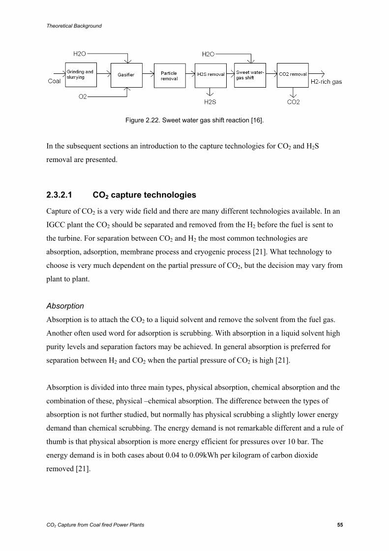
Theoretical Background
CO2 Capture from Coal fired Power Plants 55
Figure 2.22. Sweet water gas shift reaction [16].
In the subsequent sections an introduction to the capture technologies for CO2 and H2S
removal are presented.
2.3.2.1 CO2 capture technologies
Capture of CO2 is a very wide field and there are many different technologies available. In an
IGCC plant the CO2 should be separated and removed from the H2 before the fuel is sent to
the turbine. For separation between CO2 and H2 the most common technologies are
absorption, adsorption, membrane process and cryogenic process [21]. What technology to
choose is very much dependent on the partial pressure of CO2, but the decision may vary from
plant to plant.
Absorption
Absorption is to attach the CO2 to a liquid solvent and remove the solvent from the fuel gas.
Another often used word for adsorption is scrubbing. With absorption in a liquid solvent high
purity levels and separation factors may be achieved. In general absorption is preferred for
separation between H2 and CO2 when the partial pressure of CO2 is high [21].
Absorption is divided into three main types, physical absorption, chemical absorption and the
combination of these, physical –chemical absorption. The difference between the types of
absorption is not further studied, but normally has physical scrubbing a slightly lower energy
demand than chemical scrubbing. The energy demand is not remarkable different and a rule of
thumb is that physical absorption is more energy efficient for pressures over 10 bar. The
energy demand is in both cases about 0.04 to 0.09kWh per kilogram of carbon dioxide
removed [21].

Theoretical Background
CO2 Capture from Coal fired Power Plants 56
After the liquid solvent is removed from the fuel gas the CO2 is removed from the solvent.
This is done to regenerate the solvent. How to remove the carbon dioxide from the solvent
depends on what kind of absorption method used. For physical scrubbing the solvent with
CO2 must be expanded and for chemical scrubbing it must be heated. For physical-chemical
absorption the solvent is regenerated by a combination of pressure drop and increasing
temperature. This correlates with the rule of thumb that high pressure fuel gas gives incentives
for physical absorption.
Adsorption
As the word indicates adsorption has similarities with absorption. While absorption is to
attach the carbon dioxide to a liquid solvent, adsorption is to attach the CO2 to a solid solvent.
Also adsorption is divided between physical and chemical with a corresponding difference for
regenerating of the solvent. Physical adsorption has regeneration through pressure drop,
chemical adsorption has regeneration through a temperature swing and physical-chemical
adsorption has a combination of pressure drop and increasing temperature.
Adsorption has an energy demand of 0.16 to 0.20kWh per kg CO2 removed and requires very
large equipment. It is therefore only suitable for some occurrences with small gas streams
[21].
Membrane processes
A membrane separates H2 and CO2 by slipping one of the gases through and letting the other
one stay behind. As a general rule is it easier to let gases with small molecular weight through
the membrane than heavier molecules. Hydrogen has a remarkable lower molecular weight
than carbon dioxide and CO2 removal from the fuel gas is in this case therefore hydrogen
removal. Although, the hydrogen stream let through the membrane is off course the utilized
product for power production.
The main energy losses with membrane processes are the pressure drop between the two sides
of the membrane and H2 losses in CO2 stream. Hydrogen in the waste CO2 stream leads to
lesser fuel fed to turbine per amount of coal fed to the gasifier.

Theoretical Background
CO2 Capture from Coal fired Power Plants 57
Membrane processes has an energy demand of about 0.17 to 0.29kWh per kilogram of carbon
dioxide removed [21].
Cryogenic processes
A cryogenic process removes the carbon dioxide by direct condensation, sublimation or
distillation. This may be done with or without a solvent, but no solvent require low
temperature or high pressure.
Direct condensation with no solvent requires 88bar at -56°C and at 0°C the pressure must be
minimum 592bar to condensate the carbon dioxide. This is to energy demanding to be
economic feasible.
Below the triple point of carbon dioxide of -56.6°C gaseous CO2 sublimes direct into solid
state. Exxon has designed a commercial process for CO2 freezing called Controlled Freezing
Zone (CFZ). This process operates at 4bar with a temperature of -100°C and for a 90%
capture ratio the energy consumption is about 0.37kWh per kilogram of CO2 removed [21].
2.3.2.2 H2S capture technology
Removal of hydrogen sulfide is done by converting the H2S into elemental sulfur, S. To do
this the hydrogen sulfide reacts with oxygen forming elemental sulfur and water. The reaction
is shown in equation 2.49.
2 2 21/ 2H S O S H O+ → + (2.49)
This is called the Claus process and was discovered for the first time about 100 years ago.
Today it is the standard hydrogen sulfide removal procedure used in H2S scrubbers [22].
The Claus process is equal even if the H2S scrubber is placed before or after the water gas
shift reactor.
Theoretical Background
CO2 Capture from Coal fired Power Plants 58
2.4 Power Island
2.4.1 Introduction
The gasification products can be used in several industries. In this report there will be focused
on the use of syngas as fuel in power plants, IGCC. There are mainly two different fuels that
are relevant for IGCC plants depending if it is with or without CO2 capture. A power plant
without CO2 capture can use a mixture of CO and H2 from the gasifier as fuel. That differs
from plants with CO2 capture where the syngas goes through a shift reactor where conversion
to CO2 and more H2 occur. This results in a high partial pressure of CO2 which can be
removed relatively easily. The heating value part of the fuel will then exists of H2 only in
addition to some traces of CO.
The power island in an IGCC has roughly the same principles as other combined cycles where
power is generated in a gas cycle and a steam cycle. Compressed air and fuel are fed to the
gas turbine where combustion occurs and chemical energy is converted to mechanical energy.
The exhaust gas from this process is again used to run the steam cycle.
The gas cycles performance depends on the turbine inlet temperature (TIT) and the mass flow.
A higher inlet temperature at the turbine gives a higher temperature drop, which again directly
affects the change in enthalpy. There are however restrictions in how high the temperature can
be caused by the protection of the materials. A higher mass flow also increases the power
output, but also here there are limitations. These will be discussed more in 2.4.2 Turbine fired
with syngas.
The exhaust gas from the gas turbine is used to produce steam. Typical exhaust temperature is
450-650˚C and much of the energy in the exhaust gas can therefore be recovered in a heat
recovery steam generator, HRSG. In a HRSG high pressure vapor is produced at 30-120bar
with temperatures in the range of 450-560˚C. The high pressure water vapor is used in a steam
turbine to generate more power. The output pressure is typical 0.03-0.07bar [19]. After the
steam turbine the mixed phase flow enters a condenser which condenses the remaining vapor,
making the water ready to be pumped up to the mentioned high pressure. The high pressure
Theoretical Background
CO2 Capture from Coal fired Power Plants 59
water enters the HRSG and the cycle starts over. The exhaust gas is through the HRSG cooled
to 80-200˚C dependent on the size and technology of the equipment [21]. In addition to the
exhaust gas, steam can also be generated from the heat liberated in the gasification process.
The overall efficiency will then increase.
In a combined cycle power plant, the gas turbine usually contributes to about 2/3 of the total
power production and the steam turbine contributes to the remaining 1/3 [21]. When
designing combined cycles it may be a helpful rule of thumb to check if the ratios are in the
mentioned areas.
For both syngas fueled and H2 fueled turbines there are challenges compared to natural gas
fired power plant, NGCC. A short introduction to syngas and H2 fired gas turbines will be
given here. There is more available theory about syngas turbines than about H2 fired
equipment. Hydrogen fired turbines is still not a very conventional technology.
2.4.2 Turbines fired with syngas
2.4.2.1 Turbine conditions
In traditional gas turbines the fuel is premixed with air to lower the peak flame temperature
and to reduce the formation of thermal NOX. Hydrogen has a high flame propagation speed
and therefore the pre mixing is not useful for syngas turbines. There is a danger of flashback
caused by the properties of the hydrogen [20]. For IGCC application dilution of the fuel is a
method for temperature and NOX control. Typical diluters are nitrogen and water steam. An
advantage for IGCC plants are the availability of N2 from the air separation unit.
The fuel in gas fired power plants are usual a mixture where methane is the major component.
Methane has a lower heating value (LHV) of about 800MJ/kmol [19]. Mixtures of CO and H2
have a corresponding value of about 250MJ/kmol depending on the distribution between the
substances. A product stream from a gasifier also contains other substances without heating
values. This bring along an even lower volumetric LHV. The volumetric heating value for
syngas is in literature often set to only 25% of the natural gas. The consequence of this is that
a syngas turbine requires about four times higher fuel flow rate to maintain the same turbine
Theoretical Background
CO2 Capture from Coal fired Power Plants 60
inlet temperature [20]. Higher flow rate increases the power output but it can also contribute
to problems for existing turbines. This can be explained using the equation of continuity 2.50
and the ideal gas law 2.51 [16].
cm uAρ= (2.50)
Rp TM
ρ= (2.51)
With constant speed u, equation 2.52 is formed by rearranging equation 2.51 and combine it
with equation 2.50.
cMpm ART
∼ (2.52)
m = flow rate
M = molar weight
p = pressure
R = the universal gas constant
T = temperature
Ac = cross section flow area
ρ = density
The relation in 2.52 can be expanded to give the relation between a known standard condition
and another condition.
,
ref ref c
ref ref ref c ref
R T Am M pm M p R T A
= (2.53)
If the p and the T represent the inlet pressure and the inlet temperature of the turbine, one can
from this equation see the relation for a given fuel (the same M) and a constant cross section
area. Increasing in the flow rate will then either reduce the inlet temperature or increase the
inlet pressure for the turbine. The TIT is however supposed to be kept as high as possible so
the increasing in pressure is the main consequence of increasing the mass flow [20]. The inlet
pressure of the turbine is assumed to be the same as the outlet pressure of the compressor. A
higher mass flow may ergo increase the back pressure at the compressor so much that it goes
into surge. When a compressor is surging the back pressure is higher than normal and the
Theoretical Background
CO2 Capture from Coal fired Power Plants 61
pressure rate decreases. This will again reduce the air flow through the compressor [20].
When this occurs depends on the compressor surge margin which depends on the turbine type.
Another problem that may occur with syngas fuel is that the increased mass flow increases the
power output. This will directly raise the torque and the rotors have to handle with this higher
force.
When handling with natural gas compared to syngas the molecular weight M will also differ.
Pure methane has a molecular weight of about 16.04kg/kmol and a mixture of CO and H2 will
typically has a corresponding value of about 20kg/kmol. These numbers will differ a bit in
real life since natural gas is not pure methane and the syngas mixture also contains other
substances.
It should be mentioned that in a gas turbine the fuel is mixed with air with a fuel/air ratio in
the range of 0.02 for a typical natural gas fired turbine [23]. These numbers are calculated on
mass basis. That implies that the dominating part for the mass flow and the total molar
fraction is the air. A syngas fueled turbine requires a much higher fuel/air ratio. The
volumetric LHV for syngas is as mentioned about 25% of methane. The fuel/air ratio operates
on a mass basis and therefore other factors also affect the fuel/air ratio for a syngas fueled
turbine. The molar weight is higher and the need of inert gasses also contributes to a higher
fuel/air ratio. A large gas turbine can have an air flow of about 600kg/s. The total mass flow
through the turbine will for a natural gas fired turbine be given in equation 2.54.
600 600 0.02 612 kgs
⎡ ⎤+ = ⎢ ⎥⎣ ⎦i (2.54)
For a syngas fired turbine with a fuel/air ratio assumed to be 0.12 the equivalent value is
given by equation 2.55.
600 600 0.12 672 kgs
⎡ ⎤+ = ⎢ ⎥⎣ ⎦i (2.55)
From these relations one can see that the mass flow through the turbine will increase with
about 10% when the fuel is changed from natural gas to syngas.
Theoretical Background
CO2 Capture from Coal fired Power Plants 62
2.4.2.2 Modification of the equipment to handle syngas
A method to avoid surging is to increase the cross sectional area to handle a higher flow rate.
There is also a possibility to add an extra compressor stage. Then the equipment can operate
on a higher overall pressure ratio and avoid surge problems [20].
Another method is to integrate the gas turbine with the air separation unit. One can then take
some of the compressed air and send it directly to the ASU. Some of this air can be
compensated with nitrogen from the ASU. If the N2 flow is lower than the amount of air taken
from the compressor, the overall mass flow is reduced. This technology is used in the
Buggenum plant in the Netherlands [20].
2.4.3 Turbines fired with hydrogen only
One of the main challenges for IGCC plants with CO2 capture is to get turbines running on
hydrogen only. H2 turbines will reach a high temperature which is damaging for the materials.
It also has the case of moisture in the exhaust gas that also contributes to thermal challenges
caused by the physical properties of water [20]. Water has a high heat capacity, and a high
amount of water will increase the heat transfer in the turbine and put more strain on the
materials. Cooling is required to reduce the NOX formation. Use of water for cooling purpose
will increase the amount of moisture even more.
Recent developed turbines seem to handle with diluted hydrogen as fuel. Siemens has for
example their type SGT6-5000F that according to their report handles both syngas and
hydrogen [24]. This turbine has been tested for different fuel compositions and the results are
shown in table 2.7.
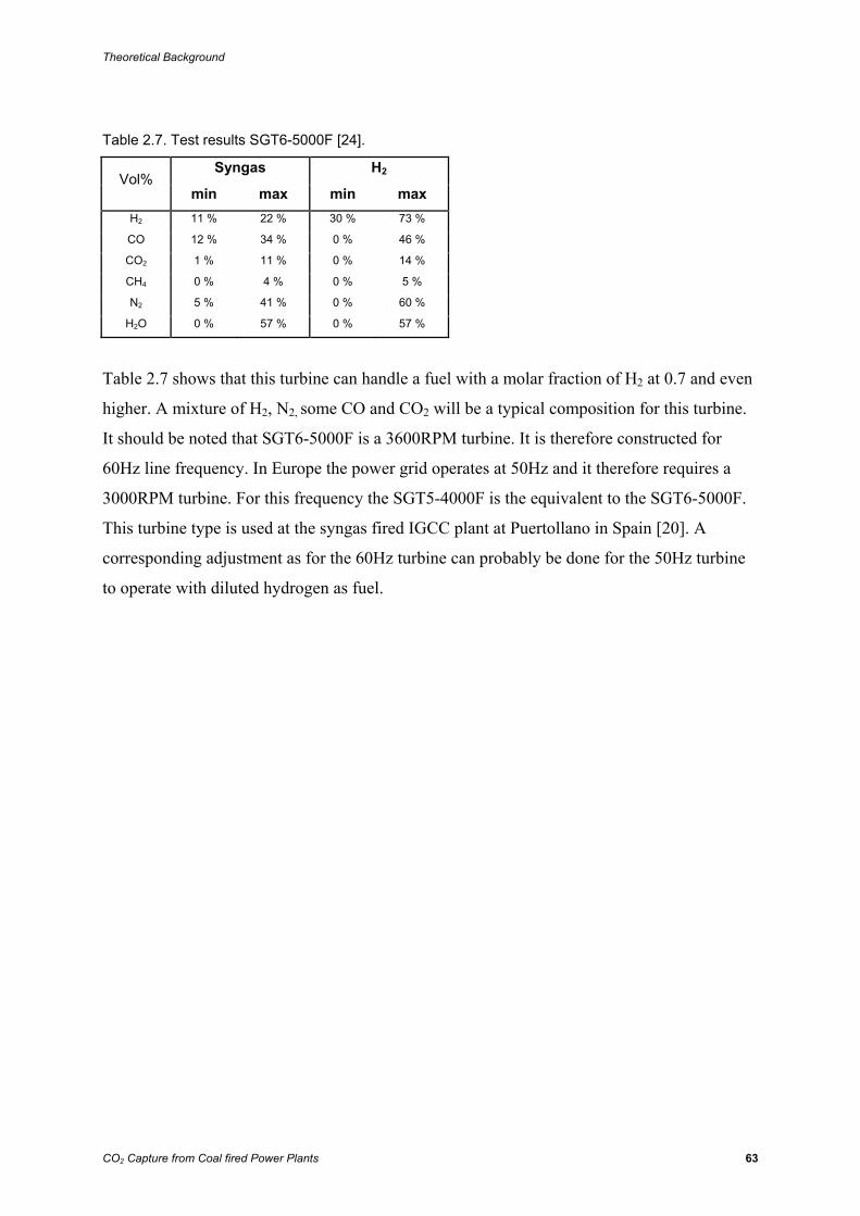
Theoretical Background
CO2 Capture from Coal fired Power Plants 63
Table 2.7. Test results SGT6-5000F [24].
Syngas H2 Vol%
min max min max H2 11 % 22 % 30 % 73 %
CO 12 % 34 % 0 % 46 %
CO2 1 % 11 % 0 % 14 %
CH4 0 % 4 % 0 % 5 %
N2 5 % 41 % 0 % 60 %
H2O 0 % 57 % 0 % 57 %
Table 2.7 shows that this turbine can handle a fuel with a molar fraction of H2 at 0.7 and even
higher. A mixture of H2, N2, some CO and CO2 will be a typical composition for this turbine.
It should be noted that SGT6-5000F is a 3600RPM turbine. It is therefore constructed for
60Hz line frequency. In Europe the power grid operates at 50Hz and it therefore requires a
3000RPM turbine. For this frequency the SGT5-4000F is the equivalent to the SGT6-5000F.
This turbine type is used at the syngas fired IGCC plant at Puertollano in Spain [20]. A
corresponding adjustment as for the 60Hz turbine can probably be done for the 50Hz turbine
to operate with diluted hydrogen as fuel.
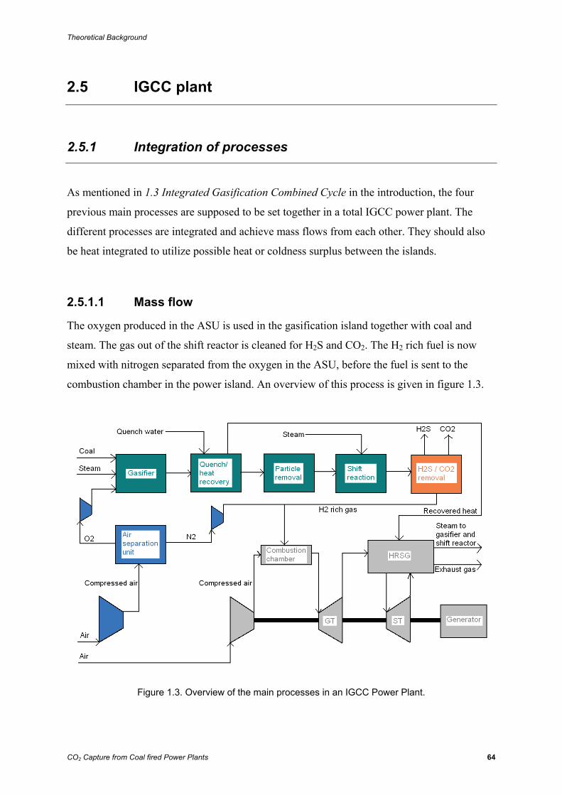
Theoretical Background
CO2 Capture from Coal fired Power Plants 64
2.5 IGCC plant
2.5.1 Integration of processes
As mentioned in 1.3 Integrated Gasification Combined Cycle in the introduction, the four
previous main processes are supposed to be set together in a total IGCC power plant. The
different processes are integrated and achieve mass flows from each other. They should also
be heat integrated to utilize possible heat or coldness surplus between the islands.
2.5.1.1 Mass flow
The oxygen produced in the ASU is used in the gasification island together with coal and
steam. The gas out of the shift reactor is cleaned for H2S and CO2. The H2 rich fuel is now
mixed with nitrogen separated from the oxygen in the ASU, before the fuel is sent to the
combustion chamber in the power island. An overview of this process is given in figure 1.3.
Figure 1.3. Overview of the main processes in an IGCC Power Plant.
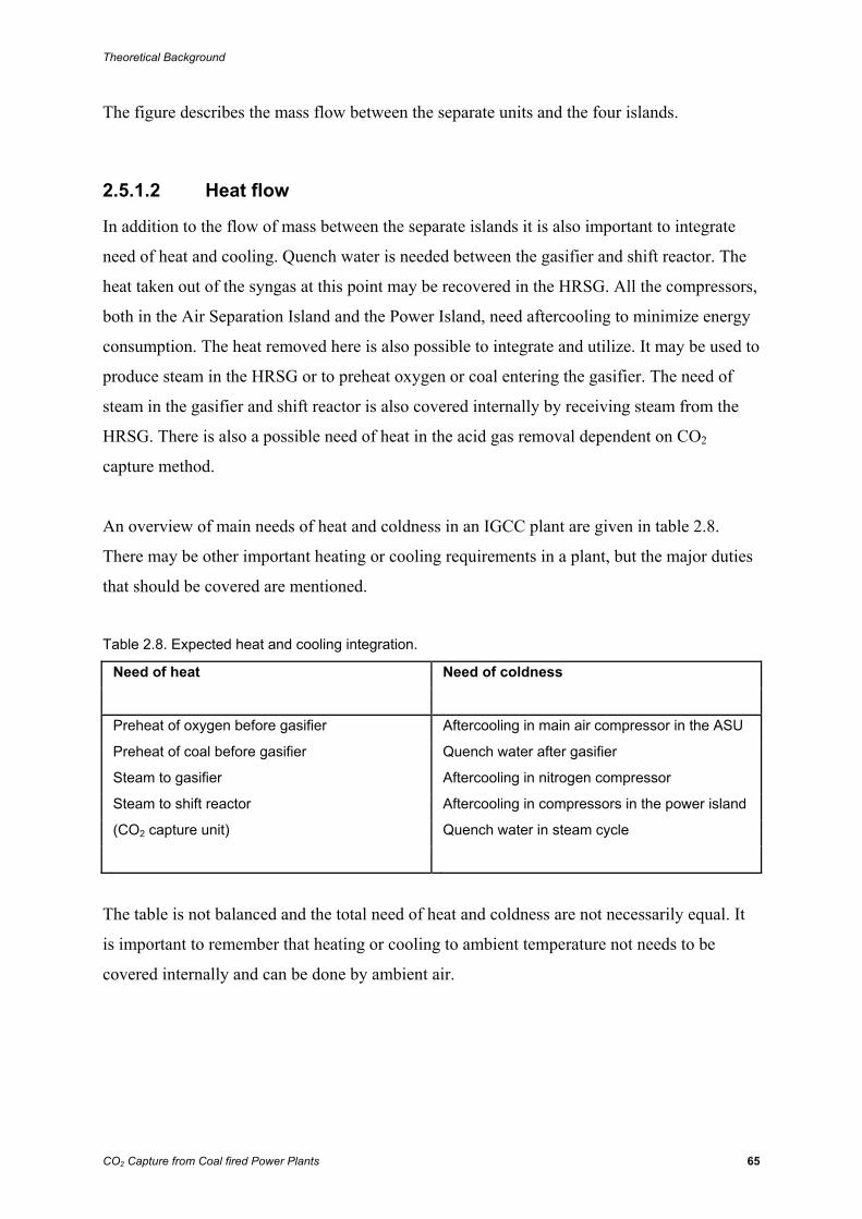
Theoretical Background
CO2 Capture from Coal fired Power Plants 65
The figure describes the mass flow between the separate units and the four islands.
2.5.1.2 Heat flow
In addition to the flow of mass between the separate islands it is also important to integrate
need of heat and cooling. Quench water is needed between the gasifier and shift reactor. The
heat taken out of the syngas at this point may be recovered in the HRSG. All the compressors,
both in the Air Separation Island and the Power Island, need aftercooling to minimize energy
consumption. The heat removed here is also possible to integrate and utilize. It may be used to
produce steam in the HRSG or to preheat oxygen or coal entering the gasifier. The need of
steam in the gasifier and shift reactor is also covered internally by receiving steam from the
HRSG. There is also a possible need of heat in the acid gas removal dependent on CO2
capture method.
An overview of main needs of heat and coldness in an IGCC plant are given in table 2.8.
There may be other important heating or cooling requirements in a plant, but the major duties
that should be covered are mentioned.
Table 2.8. Expected heat and cooling integration.
Need of heat Need of coldness
Preheat of oxygen before gasifier Aftercooling in main air compressor in the ASU
Preheat of coal before gasifier Quench water after gasifier
Steam to gasifier Aftercooling in nitrogen compressor
Steam to shift reactor Aftercooling in compressors in the power island
(CO2 capture unit) Quench water in steam cycle
The table is not balanced and the total need of heat and coldness are not necessarily equal. It
is important to remember that heating or cooling to ambient temperature not needs to be
covered internally and can be done by ambient air.
Theoretical Background
CO2 Capture from Coal fired Power Plants 66
2.5.2 Energy efficiency
Energy efficiencies in IGCC plants are not easy to find. Involved companies are careful with
information sharing and many technologies are considered company secrets. Efficiency
information available is mainly given by independent non-commercial organizations like
IPCC and IEA.
To calculate the total efficiency of an IGCC plant with CO2 capture, all the processes in the
power plant must be included. If it is assumed that the plant only generates electricity and do
not produce heat for external use equation 2.56 gives the total plant efficiency [19].
netplant
in
WQ
η = (2.56)
Wnet is the net electricity production of the power plant and Qin is the total heating value of the
fuel fed to the plant.
To calculate Wnet a total energy analysis of the plant must be done. Wnet equals the electricity
output from the generator minus all internal electricity demands. This mainly different
compressor and pump work. Qin is the lower heating value (LHV) of the fuel multiplied with
the amount fed to give the specific Wnet.
According to IPCC, a new IGCC plant with CO2 capture has typical an efficiency around
35%. Future IGCC plants of this kind may although have efficiency up to 40 percent [2]. This
is supported by the U.S Department of Energy saying the plant efficiency dependent on
technology utilized and capture ratio is ranging from around 30 to 38 percent. A typical IGCC
plant with relative high CO2 capture ratio and optimal combination of gasifier and capture
method is in the area of 36% [21].
Method
CO2 Capture from Coal fired Power Plants 67
3 Method
3.1 Air Separation Island
3.1.1 Simulation tool
The air separation island is modeled in PRO/II 8.0 by Simsci-esscor. The model is used to
calculate the energy cost of producing oxygen to the gasifier and nitrogen to dilute the fuel
before the Power Island. The needed amount of oxygen depends on the type of gasifier and
type of coal used. The need of nitrogen is not as accurate as the need of oxygen. Nitrogen is
used as a diluter and the amount mixed with the fuel is only regulating the heating value of
the fuel fed to the gas turbine. In the method part of the report the amount of oxygen and
nitrogen operates in percent of one mole of air. The modeled production of oxygen and
nitrogen are therefore measured in mole percent.
To model the air separation unit a lot of optimization and adjustments where continuous
made. This is done mainly by manually iteration. Only the major changes are presented in the
report, small adjustments and iteration steps are not shown. The final model shown in 4.1.1.6
Overall GOX considerations is although not changed after presented.
Ambient conditions are set to 298K and 1bar.
3.1.2 Gaseous oxygen
An air separation unit is modeled by stepwise expansion and manual iteration. The GOX
model is presented similar as the plant in 2.1.2 Air separation unit in the theoretical
background. The presentation of the model is following the air, oxygen and nitrogen streams
chronological and not the stepwise and iterating development of the model.
Method
CO2 Capture from Coal fired Power Plants 68
3.1.2.1 Compression
The compressor work is the only external energy input to the Air Separation Island. Cooling
water may also be looked upon as an external energy demand, but this is described in 3.1.2.3
Air cleaning. It is by this important to minimize the work done by the main compressor.
In figure 2.7 in 2.1.2.1 Introduction the compressor is drawn as one large unit. To have one
compressor handle the whole lifting work is very energy ineffective. The use of energy falls
with an increasing number of compressors. The head on each compressor is reduced and the
total work decreases. To decide the optimal number of compressors the relationship between
reduced energy input of including one extra compressor and the investment cost of this extra
compressor must be studied. This is done in 4.1.1.4 Investment cost considerations. It is
decided to use 4 compressors and in the following sections the models are presented like this.
The compression rate is decided from the pressure level in the columns. The pressure in the
columns is further decided by the temperature difference in the combined condenser and
reboiler. A pressure loss in the aftercoolers, the molecular sieves and the main heat exchanger
has to be added on to the feed pressure to the high pressure column. The pressure in the
bottom of the high pressure column is initially set to 6bar. To handle a high pressure column
feed pressure of 6bar, the compressors are set to deliver air at 6.43bars. How the pressure loss
distributes between the units before the HP column is explained when the unit is looked into.
The polytrophic efficiency was for the compressors set to 85 % [10].
3.1.2.2 Air cleaning
After compression and aftercooling the compressed air is cleaned for carbon dioxide and
moisture in the molecular sieves. Molecular sieves remove the unwanted substances by
adsorption and are not easily modeled in PRO/II. The water vapor and carbon dioxide are
therefore left out of the model and the pressure loss in molecular sieves is included in the
pressure loss in the main heat exchanger. Table 3.1 shows the simplified air composition used
in the model. The composition presented is not as accurate as the composition presented in
table 2.1, but the small derogation has neglectable impact on the air separation model
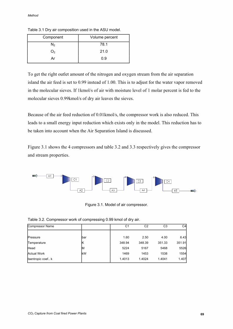
Method
CO2 Capture from Coal fired Power Plants 69
Table 3.1 Dry air composition used in the ASU model.
Component Volume percent
N2 78.1
O2 21.0
Ar 0.9
To get the right outlet amount of the nitrogen and oxygen stream from the air separation
island the air feed is set to 0.99 instead of 1.00. This is to adjust for the water vapor removed
in the molecular sieves. If 1kmol/s of air with moisture level of 1 molar percent is fed to the
molecular sieves 0.99kmol/s of dry air leaves the sieves.
Because of the air feed reduction of 0.01kmol/s, the compressor work is also reduced. This
leads to a small energy input reduction which exists only in the model. This reduction has to
be taken into account when the Air Separation Island is discussed.
Figure 3.1 shows the 4 compressors and table 3.2 and 3.3 respectively gives the compressor
and stream properties.
Figure 3.1. Model of air compressor.
Table 3.2. Compressor work of compressing 0.99 kmol of dry air. Compressor Name C1 C2 C3 C4
Pressure bar 1.60 2.50 4.00 6.43
Temperature K 348.94 348.39 351.33 351.91
Head M 5224 5167 5468 5526
Actual Work kW 1469 1453 1538 1554
Isentropic coef.. k 1.4013 1.4024 1.4041 1.407
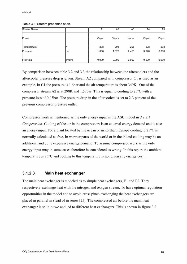
Method
CO2 Capture from Coal fired Power Plants 70
Table 3.3. Stream properties of air. Stream Name A1 A2 A3 A4 A5
Phase Vapor Vapor Vapor Vapor Vapor
Temperature K 298 298 298 298 298
Pressure bar 1.000 1,570 2,450 3,920 6,300
Flowrate kmol/s 0,990 0,990 0,990 0,990 0,990
By comparison between table 3.2 and 3.3 the relationship between the aftercoolers and the
aftercooler pressure drop is given. Stream A2 compared with compressor C1 is used as an
example. In C1 the pressure is 1.6bar and the air temperature is about 349K. Out of the
compressor stream A2 is at 298K and 1.57bar. This is equal to cooling to 25°C with a
pressure loss of 0.03bar. The pressure drop in the aftercoolers is set to 2-3 percent of the
previous compressor pressure outlet.
Compressor work is mentioned as the only energy input in the ASU model in 3.1.2.1
Compression. Cooling of the air in the compressors is an external energy demand and is also
an energy input. For a plant located by the ocean or in northern Europe cooling to 25°C is
normally calculated as free. In warmer parts of the world or in the inland cooling may be an
additional and quite expensive energy demand. To assume compressor work as the only
energy input may in some cases therefore be considered as wrong. In this report the ambient
temperature is 25°C and cooling to this temperature is not given any energy cost.
3.1.2.3 Main heat exchanger
The main heat exchanger is modeled as to simple heat exchangers, E1 and E2. They
respectively exchange heat with the nitrogen and oxygen stream. To have optimal regulation
opportunities in the model and to avoid cross pinch exchanging the heat exchangers are
placed in parallel in stead of in series [25]. The compressed air before the main heat
exchanger is split in two and led to different heat exchangers. This is shown in figure 3.2.
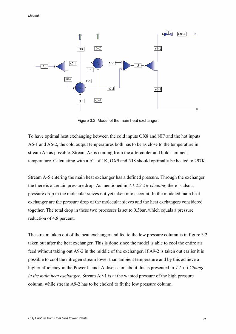
Method
CO2 Capture from Coal fired Power Plants 71
Figure 3.2. Model of the main heat exchanger.
To have optimal heat exchanging between the cold inputs OX8 and NI7 and the hot inputs
A6-1 and A6-2, the cold output temperatures both has to be as close to the temperature in
stream A5 as possible. Stream A5 is coming from the aftercooler and holds ambient
temperature. Calculating with a ΔT of 1K, OX9 and NI8 should optimally be heated to 297K.
Stream A-5 entering the main heat exchanger has a defined pressure. Through the exchanger
the there is a certain pressure drop. As mentioned in 3.1.2.2 Air cleaning there is also a
pressure drop in the molecular sieves not yet taken into account. In the modeled main heat
exchanger are the pressure drop of the molecular sieves and the heat exchangers considered
together. The total drop in these two processes is set to 0.3bar, which equals a pressure
reduction of 4.8 percent.
The stream taken out of the heat exchanger and fed to the low pressure column is in figure 3.2
taken out after the heat exchanger. This is done since the model is able to cool the entire air
feed without taking out A9-2 in the middle of the exchanger. If A9-2 is taken out earlier it is
possible to cool the nitrogen stream lower than ambient temperature and by this achieve a
higher efficiency in the Power Island. A discussion about this is presented in 4.1.1.3 Change
in the main heat exchanger. Stream A9-1 is at the wanted pressure of the high pressure
column, while stream A9-2 has to be choked to fit the low pressure column.
Method
CO2 Capture from Coal fired Power Plants 72
Since air is a non ideal gas, choking between A9-2 and A10-2 causes a temperature fall in the
stream [19]. The choking is done in a valve and adjusts the pressure to low pressure column
pressure. The pressure may also be reduced by an expander. An expander will lead to an even
lower temperature at A10-2 and does also produce a small energy amount that may be
utilized. Use of valve or expander is also closely connected to the topic of where in the heat
exchanger A9-2 is taken out. As mentioned above, a closer analysis of this is presented in
4.1.1.3 Change in the main heat exchanger.
3.1.2.4 High pressure column
Stream A9-1 enters the bottom tray of the high pressure column at 6bar. The column has a
pressure drop upwards the column and the pressure drop is set to 0.5bar. The condenser in the
column makes it advantageous to specify the nitrogen purity in the stream leaving the
condenser. This purity is set to be 99 percent and the condenser duty is varied by PRO/II to
achieve this. At the bottom of the column an oxygen rich stream leaves the column, but no
specifications of purity or mass rate are made for this stream. The mentioned pressure
assumption gives a pressure at 5.5bar in the top stream and 6bar in the bottom stream.
It also has to be decided on how many trays needed to achieve the wanted separation. To
decide the tray number the column is initially set to have 40 trays. This is probably too many
trays, but with a conservative assumption it is easier to adjust the number of trays to an
optimal level afterwards. Figure 3.3 shows the separation factor plotted against the number of
trays. The figure is plotted in PRO/II.
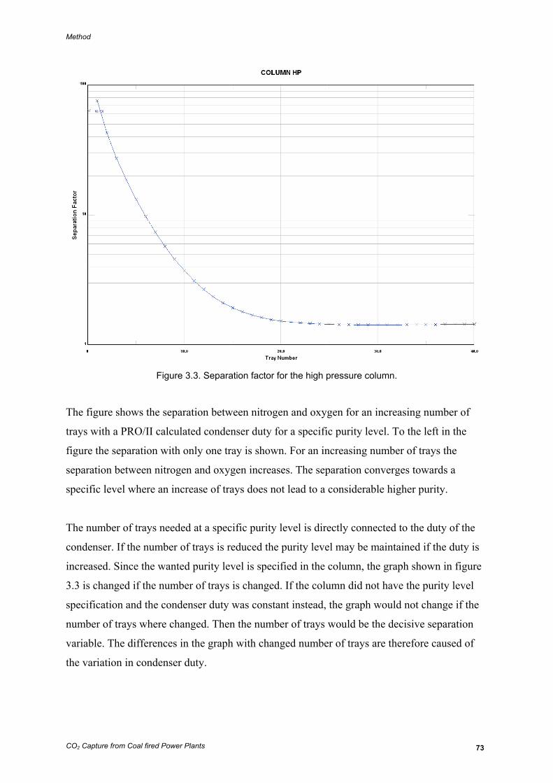
Method
CO2 Capture from Coal fired Power Plants 73
Figure 3.3. Separation factor for the high pressure column.
The figure shows the separation between nitrogen and oxygen for an increasing number of
trays with a PRO/II calculated condenser duty for a specific purity level. To the left in the
figure the separation with only one tray is shown. For an increasing number of trays the
separation between nitrogen and oxygen increases. The separation converges towards a
specific level where an increase of trays does not lead to a considerable higher purity.
The number of trays needed at a specific purity level is directly connected to the duty of the
condenser. If the number of trays is reduced the purity level may be maintained if the duty is
increased. Since the wanted purity level is specified in the column, the graph shown in figure
3.3 is changed if the number of trays is changed. If the column did not have the purity level
specification and the condenser duty was constant instead, the graph would not change if the
number of trays where changed. Then the number of trays would be the decisive separation
variable. The differences in the graph with changed number of trays are therefore caused of
the variation in condenser duty.
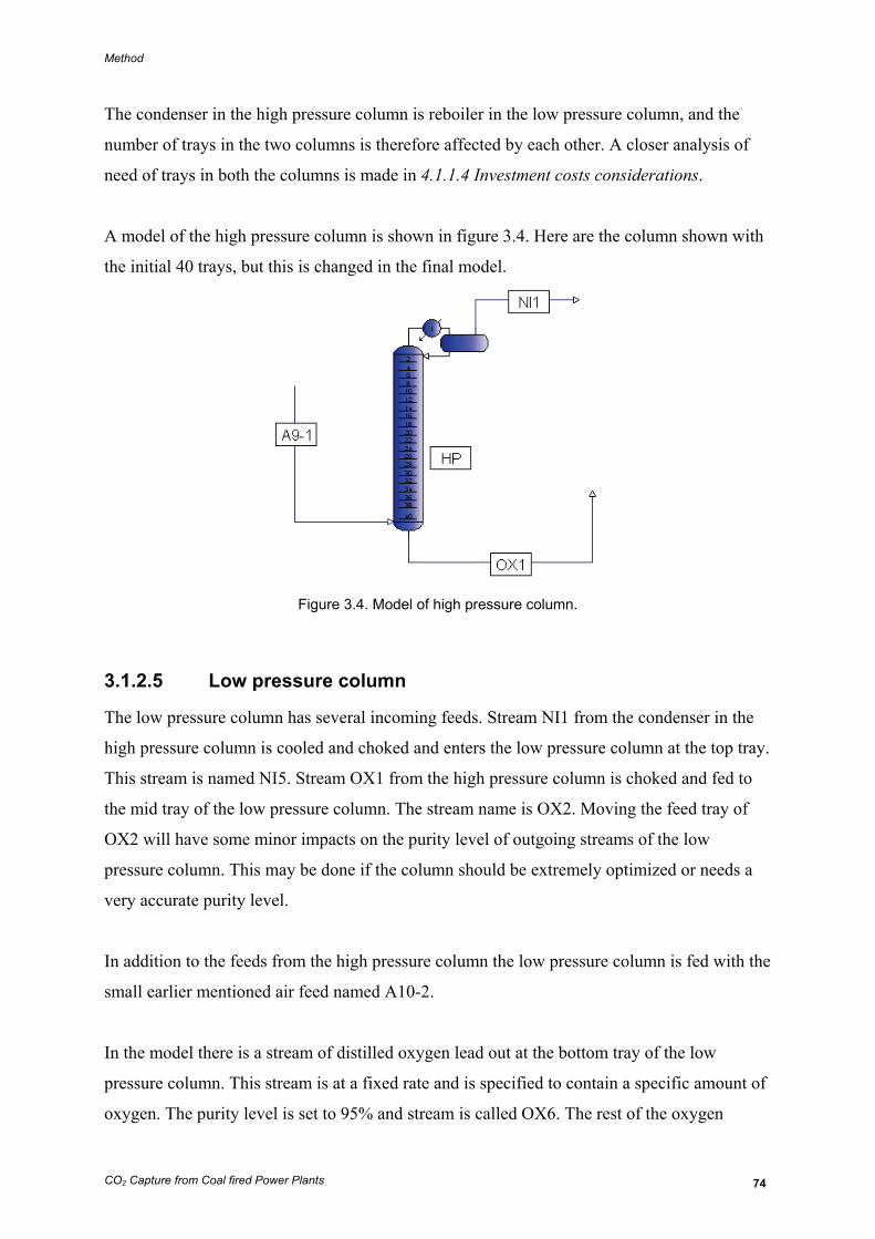
Method
CO2 Capture from Coal fired Power Plants 74
The condenser in the high pressure column is reboiler in the low pressure column, and the
number of trays in the two columns is therefore affected by each other. A closer analysis of
need of trays in both the columns is made in 4.1.1.4 Investment costs considerations.
A model of the high pressure column is shown in figure 3.4. Here are the column shown with
the initial 40 trays, but this is changed in the final model.
Figure 3.4. Model of high pressure column.
3.1.2.5 Low pressure column
The low pressure column has several incoming feeds. Stream NI1 from the condenser in the
high pressure column is cooled and choked and enters the low pressure column at the top tray.
This stream is named NI5. Stream OX1 from the high pressure column is choked and fed to
the mid tray of the low pressure column. The stream name is OX2. Moving the feed tray of
OX2 will have some minor impacts on the purity level of outgoing streams of the low
pressure column. This may be done if the column should be extremely optimized or needs a
very accurate purity level.
In addition to the feeds from the high pressure column the low pressure column is fed with the
small earlier mentioned air feed named A10-2.
In the model there is a stream of distilled oxygen lead out at the bottom tray of the low
pressure column. This stream is at a fixed rate and is specified to contain a specific amount of
oxygen. The purity level is set to 95% and stream is called OX6. The rest of the oxygen
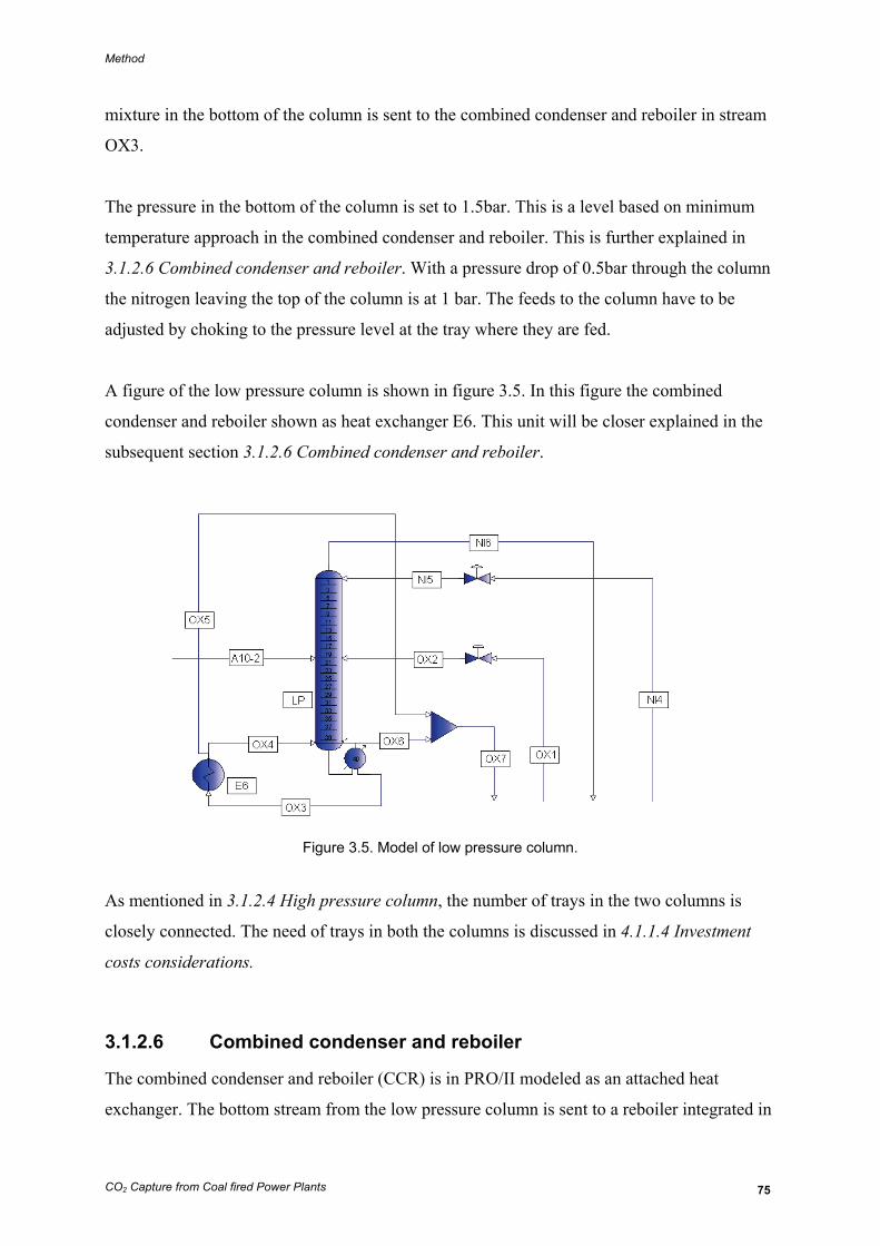
Method
CO2 Capture from Coal fired Power Plants 75
mixture in the bottom of the column is sent to the combined condenser and reboiler in stream
OX3.
The pressure in the bottom of the column is set to 1.5bar. This is a level based on minimum
temperature approach in the combined condenser and reboiler. This is further explained in
3.1.2.6 Combined condenser and reboiler. With a pressure drop of 0.5bar through the column
the nitrogen leaving the top of the column is at 1 bar. The feeds to the column have to be
adjusted by choking to the pressure level at the tray where they are fed.
A figure of the low pressure column is shown in figure 3.5. In this figure the combined
condenser and reboiler shown as heat exchanger E6. This unit will be closer explained in the
subsequent section 3.1.2.6 Combined condenser and reboiler.
Figure 3.5. Model of low pressure column.
As mentioned in 3.1.2.4 High pressure column, the number of trays in the two columns is
closely connected. The need of trays in both the columns is discussed in 4.1.1.4 Investment
costs considerations.
3.1.2.6 Combined condenser and reboiler
The combined condenser and reboiler (CCR) is in PRO/II modeled as an attached heat
exchanger. The bottom stream from the low pressure column is sent to a reboiler integrated in
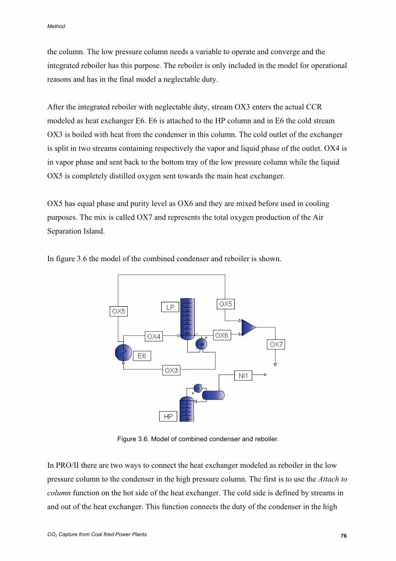
Method
CO2 Capture from Coal fired Power Plants 76
the column. The low pressure column needs a variable to operate and converge and the
integrated reboiler has this purpose. The reboiler is only included in the model for operational
reasons and has in the final model a neglectable duty.
After the integrated reboiler with neglectable duty, stream OX3 enters the actual CCR
modeled as heat exchanger E6. E6 is attached to the HP column and in E6 the cold stream
OX3 is boiled with heat from the condenser in this column. The cold outlet of the exchanger
is split in two streams containing respectively the vapor and liquid phase of the outlet. OX4 is
in vapor phase and sent back to the bottom tray of the low pressure column while the liquid
OX5 is completely distilled oxygen sent towards the main heat exchanger.
OX5 has equal phase and purity level as OX6 and they are mixed before used in cooling
purposes. The mix is called OX7 and represents the total oxygen production of the Air
Separation Island.
In figure 3.6 the model of the combined condenser and reboiler is shown.
Figure 3.6. Model of combined condenser and reboiler.
In PRO/II there are two ways to connect the heat exchanger modeled as reboiler in the low
pressure column to the condenser in the high pressure column. The first is to use the Attach to
column function on the hot side of the heat exchanger. The cold side is defined by streams in
and out of the heat exchanger. This function connects the duty of the condenser in the high

Method
CO2 Capture from Coal fired Power Plants 77
pressure column to the duty delivered on hot side of the exchanger. The other is to define a
FORTRAN subroutine in the specification of the heat exchanger. In the modeled developed
for this report the Attach to column function is used.
When using the Attach to column function it is important to be aware of the minimum
temperature approach, ΔT. The Attach to column function only use the duty in the condenser
to boil stream OX3 without concerning about temperatures. A model with heat transferred
from cold to hot side would therefore be operational in PRO/II with this function. This is not
legal according to the second law of thermodynamics and the temperature difference needs to
be taken care of manually. With a ΔT value of 1K the stream OX3 always has to be 1K below
the temperature out of the condenser. This temperature is equal to the temperature of NI1. For
the island to be operational in real life NI1 must always be at least 1K above OX3.
The parameters deciding the temperature of NI1 and OX3 is the top pressure of the high
pressure column and the bottom pressure of the low pressure column. NI1 is directly
dependent on the pressure in the condenser as long as the purity level is defined. Likewise is
OX3 directly dependent on the pressure in the reboiler for a specific purity level. With
nitrogen purity of minimum 99% in NI1 and oxygen purity of minimum 95% in OX3 the
pressure in the columns directly decides the temperatures.
A change in purity level will not have major impacts on the temperatures, but in a system with
very small temperature differences it is important to be aware of the great sensitivity.
3.1.2.7 Subcooler
The nitrogen stream leaving the high pressure column needs to be cooled before entering the
low pressure column. This is done in heat exchanger E3 and E4. They are not a part of the
main heat exchanger and may be considered as a subcooler for the nitrogen stream. This is
shown in figure 3.7.
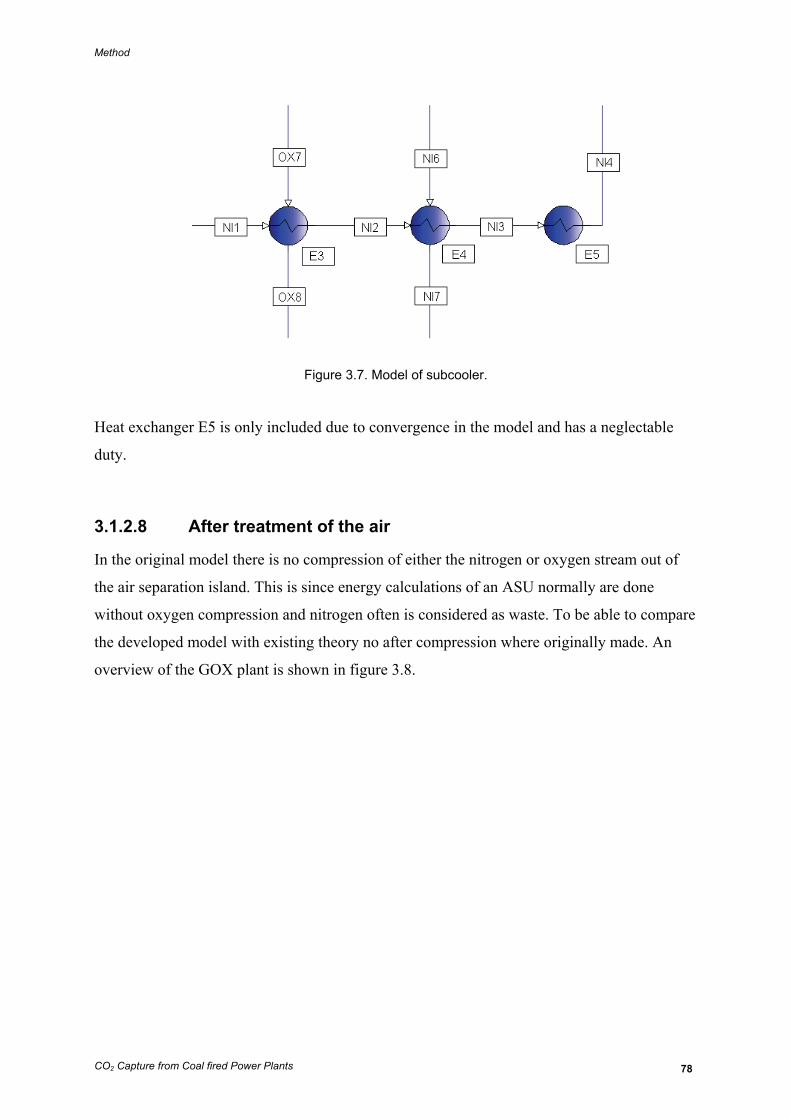
Method
CO2 Capture from Coal fired Power Plants 78
Figure 3.7. Model of subcooler.
Heat exchanger E5 is only included due to convergence in the model and has a neglectable
duty.
3.1.2.8 After treatment of the air
In the original model there is no compression of either the nitrogen or oxygen stream out of
the air separation island. This is since energy calculations of an ASU normally are done
without oxygen compression and nitrogen often is considered as waste. To be able to compare
the developed model with existing theory no after compression where originally made. An
overview of the GOX plant is shown in figure 3.8.

Method
CO2 Capture from Coal fired Power Plants 79
Figure 3.8. Model of GOX plant without oxygen compression.
To compare a GOX island with a LOX island the oxygen in both cases needs to be
compressed to a wanted level. To compare the developed GOX and LOX models with each
other and given literature, compressors are added on OX9.
In the final model used for energy considerations for a total power plant, compression of both
the oxygen used for gasification and nitrogen used to dilute the fuel are compressed to a
desirable level. The oxygen feed to the gasifier has a pressure level at 42bar and the fuel feed
to the turbine has a pressure level at about 26bar.
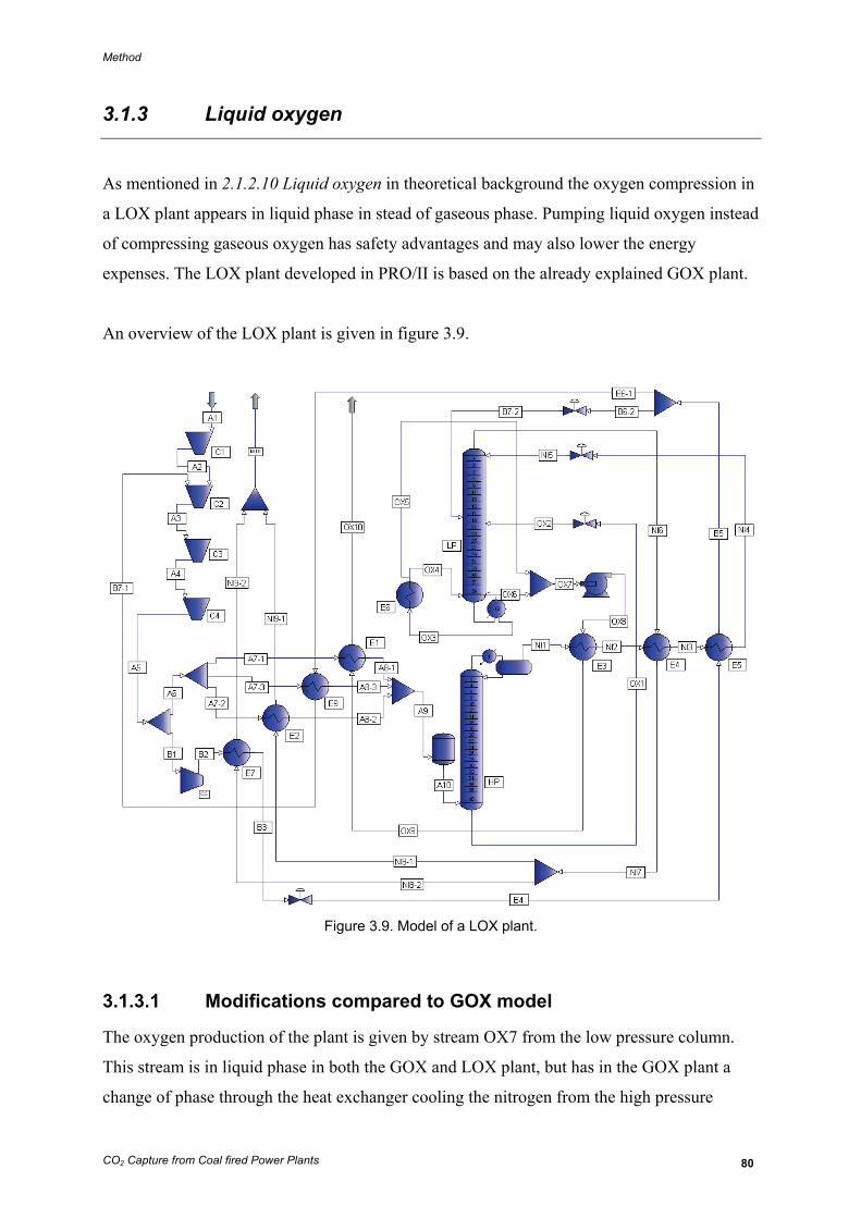
Method
CO2 Capture from Coal fired Power Plants 80
3.1.3 Liquid oxygen
As mentioned in 2.1.2.10 Liquid oxygen in theoretical background the oxygen compression in
a LOX plant appears in liquid phase in stead of gaseous phase. Pumping liquid oxygen instead
of compressing gaseous oxygen has safety advantages and may also lower the energy
expenses. The LOX plant developed in PRO/II is based on the already explained GOX plant.
An overview of the LOX plant is given in figure 3.9.
Figure 3.9. Model of a LOX plant.
3.1.3.1 Modifications compared to GOX model
The oxygen production of the plant is given by stream OX7 from the low pressure column.
This stream is in liquid phase in both the GOX and LOX plant, but has in the GOX plant a
change of phase through the heat exchanger cooling the nitrogen from the high pressure

Method
CO2 Capture from Coal fired Power Plants 81
column. At the entrance of E1 in the main heat exchanger the oxygen stream is in vapor
phase.
In the LOX plant a pump is installed before the heat exchanging in E3 which causes phase
change. Stream OX7 is therefore pumped to wanted pressure before entering heat exchanger
E3. Because of the pressure rise there is no change of phase through heat exchanger E3. This
leads to a very low heat exchanging in heat exchanger E3 and a subsequent need of cooling in
the nitrogen stream between the high pressure and low pressure column. The oxygen stream
entering the main heat exchanger in E1 is now in liquid phase and the phase change appears
through this exchanger.
The need of cooling in the nitrogen stream between the high pressure and low pressure
column must be covered by an internal made increase in heat removed from the island. This is
done by installing a splitter after the main compressor and compress parts of the air further.
The air is sent through heat exchanger E7, which is a part of the main heat exchanger, before
it is choked to achieve more coldness. The coldness is then used to cool the nitrogen stream
between the high pressure and low pressure column by heat exchanger E5.
3.1.3.2 Minimum temperature approach problems
As presented in the theoretical background the booster compressed air is choked to a pressure
equal to high pressure column pressure. In the model developed for this report, it is not
possible to cool the nitrogen stream with air at high pressure column pressure. If the air is
choked to high pressure column level the temperature in the air is higher than the temperature
in the nitrogen stream. This is shown in table 3.4.
Table 3.4. Stream properties for nitrogen from condenser and boosted air.
Stream Name NI3 B4 – 6.00bar B4 – 1.57bar
Phase Mixed Mixed Mixed
Temperature K 95.305 98.543 83.336
Pressure bar 5.500 6.000 1.570
Flowrate kmol/s 0.429 0.300 0.300
Composition
O2 0.005 0.210 0.210
N2 0.990 0.781 0.781
AR 0.005 0.009 0.009
Method
CO2 Capture from Coal fired Power Plants 82
Air in mixed phase at 6bar, B4 – 6.0bar, has a higher temperature than the nitrogen that need
to be cooled, NI3. One solution is to cool air at 6bar to a temperature which makes it possible
to heat exchange with NI3. Because air is in mixed phase and has its critical temperature at
98.543K at 6bar, this would demand an unacceptable energy amount. To be able to cool NI3
the air needs to be choked further, to a pressure level lower than the high pressure column.
If the air is choked lower than the pressure level in the high pressure column it can not be fed
directly to the high pressure column. The solution for this is to feed parts of the air to the low
pressure column and recompress the rest. The recompression may either be done by an extra
compressor, by mixing the low pressured air stream with booster compressed air to a suitable
pressure level, or by feeding the air back to the main compressor. The most energy efficient
solution is to feed the low pressured air back to the main compressor. Without need of extra
compressors this is also a less maintenance demanding.
At what pressure B4 should be choked to is dependent on the energy amount that needs to be
exchanged with NI3 and how the pressure should be increased again afterwards. Because of
the energy that need to be exchanged between NI3 and B4 it was found out that the pressure
had to be equal to or below 2bar. To match one of the steps in the main air compressor for
recompression the pressure is set to 1.57bar, see table 3.2 and 3.3. Stream properties of
boosted air is shown as B4 – 1.5bar in table 3.4.
In the GOX model, heat exchanger E5 is independent and included for the model to converge.
Heat exchanger E5 is in the LOX model integrated and the duty is covered internally. The
flash tank before the high pressure column is therefore included to have an independent unit
"helping" the model converge. The purpose of the flash tank is to set the temperature of the
outgoing air stream to dew point. This flash tank may be seen as a heat exchanger setting the
temperature of the stream to dew point. The air stream entering the flash tank is very near dew
point and the duty of the tank is neglectable. It is possible to run the model without the flash
tank, but even minor input changes then leads to convergence problems.

Method
CO2 Capture from Coal fired Power Plants 83
3.1.4 Argon treatment
Argon removal is not handled in the developed models. The slightly raised purity level in the
oxygen and nitrogen achieved by removal of argon has no major improvements on either the
Gasification Island or the Power Island. To justify implementation of an argon column in an
ASU for IGCC purpose, the argon captured has to be sold at an acceptable price. This report
does not focus on economic profits by operating in the argon market and the additional
column is therefore not implemented.
Method
CO2 Capture from Coal fired Power Plants 84
3.2 Gasification Island
3.2.1 Simulation tools
The Gasification Island is also simulated in PRO/II 8.0.
PRO/II is normally used for fluids and the first approach is to verify if the program could
handle solid fuels like coal. There are run simulations on a self made coal composition and on
a structure where coal is defined as a gas. The testing of PRO/II was a part of the project work
during autumn 2007. A short repetition of this work is presented here. Thereafter modeling of
different coal types is presented.
There are also done calculations in MatLab version R2007a. The calculations performed are
equilibrium calculations on the gasification procedure. This is done to solve a gasification
problem from simple formation reactions to finished syngas composition.
In addition to MatLab and PRO/II, an online chemical equilibrium calculator is used [26].
This tool is utilized to check the validity of simulations and calculations performed.
3.2.2 MatLab calculations
The formation reactions are the heart of the gasifier. From the formation reactions together
with mass balances, a set of equations giving the syngas composition may be derived. To
solve such a complex equation set the mathematical computer tool MatLab is used.
Calculating a syngas composition in MatLab demands manually equation derivation. MatLab
is only an equation solver and the derivation from formation reaction to a solvable equation
set is done manually. The reason for doing this is to show that the results calculated from
simple formation reactions corresponds to calculated values from more advanced computer
tools as PRO/II and the chemical equilibrium calculator.
Method
CO2 Capture from Coal fired Power Plants 85
3.2.2.1 Complete equation set
From the formation reactions presented in the theoretical background it is possible to calculate
the syngas composition. The conversion of coal, oxygen and steam to syngas is decided by
these formation reactions together with input values as temperature, pressure and coal
composition. The coal composition is assumed to be a combination of C, H, O, N and S. The
seven independent formation reactions are presented in 2.2.2.1 Formation reactions and are
repeated below.
21 2C O CO+ -111 MJ/kmol (2.30)
2 2C O CO+ → -394 MJ/kmol (2.31)
2 42C H CH+ -75 MJ/kmol (2.33)
2 2 21 2H O H O+ -242 MJ/kmol (2.35)
2 21 2 1 2N O NO+ +90 MJ/kmol (2.36)
2 2S O SO+ -362 MJ/kmol (2.37)
2 2S H H S+ -85 MJ/kmol (2.38)
The reactions contain a total of 12 substances. In theory traces of all 12 substances is found in
the syngas composition and the equation set therefore contains a minimum of 12 unknown. In
calculations it is not necessary to include all 12 substances in the equilibrium. This is due to
neglectable amount of several of the substances. A method containing all 12 substances is
although presented before the set of equations is reduced to containing only the relevant ones.
All the reactions have belonging equilibrium equations presented in chapter 2.2.2.2
Equilibrium equations. The equilibrium equations are derived from the formation reactions
and the deriving procedure is described in Appendix A. The equilibrium equations are
repeated below.
[ ]
2
1122
COCO
C O
yK
y y p=⎡ ⎤ ⎡ ⎤⎣ ⎦ ⎣ ⎦
(2.40)
2
2
2
COCO
C O
yK
y y p
⎡ ⎤⎣ ⎦=⎡ ⎤ ⎡ ⎤⎣ ⎦ ⎣ ⎦
(2.41)
Method
CO2 Capture from Coal fired Power Plants 86
2
2
2 2
12
H OH O
H O
yK
y y p
⎡ ⎤⎣ ⎦=⎡ ⎤ ⎡ ⎤⎣ ⎦ ⎣ ⎦
(2.42)
4
4
2
2 2
CHCH
C H
yK
y y p
⎡ ⎤⎣ ⎦=⎡ ⎤ ⎡ ⎤⎣ ⎦ ⎣ ⎦
(2.43)
[ ]
2 2
1 12 2
NONO
O N
yK
y y=⎡ ⎤ ⎡ ⎤⎣ ⎦ ⎣ ⎦
(2.44)
2
2
2
SOSO
S O
yK
y y p
⎡ ⎤⎣ ⎦=⎡ ⎤ ⎡ ⎤⎣ ⎦ ⎣ ⎦
(2.45)
2
2
2
H SH S
S H
yK
y y p
⎡ ⎤⎣ ⎦=⎡ ⎤ ⎡ ⎤⎣ ⎦ ⎣ ⎦
(2.46)
The 12 unknown molar fractions are implemented in equation 2.40 to 2.46. Equation 2.40 to
2.46 are also the first 7 equations in the equation set. The equilibrium constants K are
tabulated for given temperatures.
The element mass balances for the five feed substances are independent equations and are
implemented in the equation set. An element mass balance equation gives that the amount of
an element fed to a process must equal the amount of the element going out of the process. If
1kmol/s of C is fed to the gasifier the sum of C, CO, CO2 and CH4 also must equal to
1kmol/s. In this process there are five elements in the feed giving five element mass balances.
2 4( )
FeedC C CO CO CHy y y y y n= + + + (3.1)
4 2 2 2(4 2 2 2 )
FeedH CH H H O H Sy y y y y n= + + + (3.2)
2 2 2 2( 2 2 0.5 2 )
FeedO CO CO O H O NO SOy y y y y y y n= + + + + + (3.3)
2(2 )
FeedN N NOy y y n= + (3.4)
2 2( )
FeedS S SO H Sy y y y n= + + (3.5)
C, N and S are in theory fed to the gasifier process only through the coal. H and O are fed
both through the coal and through the feeds of oxygen and steam. When calculating the
element feeds it is therefore important to include the H and O feed from steam and oxygen in
Method
CO2 Capture from Coal fired Power Plants 87
addition to the feed from the coal. If the calculation should be extremely precise the few
percent of nitrogen in the oxygen feed from the ASU and possible pollution in the water also
needs to be taken into account.
The equation set now contains 12 equations, but the introduction of the variable giving the
total number of moles in the equilibrium gas mixture, n, makes need for an extra equation.
This is solved by the equation of the total mass balance.
2 4 2 2 2 2 2 2
1C CO CO CH O H H O N NO S SO H Sy y y y y y y y y y y y+ + + + + + + + + + + = (3.6)
The equation set now contains 13 equations with 13 unknown.
3.2.2.2 Reduction of the equation set
The equation set containing 13 equations and 13 unknown is very complex to solve. In fact,
the extremely small amount of some of the substances makes a MatLab model not able to
solve the equation set. When the molar fractions get this close to zero and other mole fractions
are divided by these the model is unsolvable. The solution is to reduce the set of equations to
a set containing only the substances with practical influence of the syngas composition.
The amount of CH4, NO, H2S and SO2 are considered to small to have major impact on the
syngas composition. The remaining independent formation reactions are then 2.30, 2.31 and
2.35.
21 2C O CO+ (2.30)
2 2C O CO+ → (2.31)
2 2 21 2H O H O+ (2.35)
This assumption also gives that there is no nitrogen or sulfur in the coal composition. This is a
simplification need to be done to get the MatLab model to converge. The coal is then
containing of a combination of carbon, hydrogen and oxygen.
Method
CO2 Capture from Coal fired Power Plants 88
It is also assumed that all the oxygen is consumed in the gasification process and there is no
oxygen left in the syngas. This reduces the three independent formation reactions to two new
formation reactions. These reactions are independent of each other, but are dependent of the
previous three.
The first new formation reaction, 2.32, is derived by subtracting 2.31 from 2.30 multiplied
with two.
2 2C CO CO+ (2.32)
The other new formation reaction, 2.24, is derived by subtracting 2.35 from 2.30.
2 2C H O CO H+ + (2.34)
It is further assumed that all the carbon is gasified and there is no pure carbon left in the
syngas. In real life some of the carbon is not gasified and leaves the gasifier together with ash
and slag. It is although a legal approximation assuming no carbon in the syngas.
Subtraction of 2.34 from 2.32 gives a formation reaction without pure carbon.
2 2 2CO H O CO H+ + (3.10)
From 3.10 the following equilibrium constant can be set up.
2 2
2
CO H
CO H O
y yK
y y
⎡ ⎤ ⎡ ⎤⎣ ⎦ ⎣ ⎦=⎡ ⎤ ⎡ ⎤⎣ ⎦ ⎣ ⎦
(3.11)
Equation 3.11 contains five unknown. First of all the K value is derived.
[ ]2
2
1122
2 1122
1 2 COCO CO CO C O
C O
yC O CO K y K y y p
y y p⎡ ⎤ ⎡ ⎤ ⎡ ⎤+ ⇒ = ⇒ =⎣ ⎦ ⎣ ⎦ ⎣ ⎦
⎡ ⎤ ⎡ ⎤⎣ ⎦ ⎣ ⎦
(3.12)
Method
CO2 Capture from Coal fired Power Plants 89
2
2 2 2 2
2
2 2CO
CO CO CO C OC O
yC O CO K y K y y p
y y p
⎡ ⎤⎣ ⎦ ⎡ ⎤ ⎡ ⎤ ⎡ ⎤+ → ⇒ = ⇒ =⎣ ⎦ ⎣ ⎦ ⎣ ⎦⎡ ⎤ ⎡ ⎤⎣ ⎦ ⎣ ⎦ (3.13)
2
2 2 2 2 2
2 2
12
2 2 2 12
1 2 H OH O H O H O H O
H O
yH O H O K y K y y p
y y p
⎡ ⎤⎣ ⎦ ⎡ ⎤ ⎡ ⎤ ⎡ ⎤+ ⇒ = ⇒ =⎣ ⎦ ⎣ ⎦ ⎣ ⎦⎡ ⎤ ⎡ ⎤⎣ ⎦ ⎣ ⎦
(3.14)
The K value is found by inserting 3.12, 3.13 and 3.14 in 3.11.
2 2 2 2 2 2
222 2 2 2
1 112 22
CO H CO C O H CO
CO H OCO H OCO C O H O H O
y y K y y p y KK
K Ky y K y y p K y y p
⎡ ⎤ ⎡ ⎤ ⎡ ⎤ ⎡ ⎤ ⎡ ⎤⎣ ⎦ ⎣ ⎦ ⎣ ⎦ ⎣ ⎦ ⎣ ⎦= = =⎡ ⎤ ⎡ ⎤⎣ ⎦ ⎣ ⎦ ⎡ ⎤ ⎡ ⎤ ⎡ ⎤ ⎡ ⎤⎣ ⎦ ⎣ ⎦ ⎣ ⎦ ⎣ ⎦
i (3.15)
This gives an equation with four unknown.
2 22
2 2
CO HCO
CO H O CO H O
y yKK K y y
⎡ ⎤ ⎡ ⎤⎣ ⎦ ⎣ ⎦=⎡ ⎤ ⎡ ⎤⎣ ⎦ ⎣ ⎦i
(3.16)
KCO2, KCO and KH2O are tabulated for specific temperatures. In some literature the equilibrium
constant in equation 3.11 are tabulated directly and the derivations performed in 3.12 to 3.16
are not necessary. It is although shown here to give the entire derivation from the elementary
formation reaction to the calculated syngas composition.
The next three equations are given by element mass balance and form a new unknown, n.
2( )
FeedC CO COy y y n= + (3.17)
2 2(2 2 )
FeedH H H Oy y y n= + (3.18)
2 2( 2 0.5 )
FeedO CO CO H Oy y y y n= + + (3.19)
Here is yC,Feed the number of moles of carbon in the coal. yH,Feed is moles of hydrogen in the
coal plus the moles of steam multiplied with two. The addition of two times the number of
moles of steam is to add on the two hydrogen atoms in H2O. Equally yO,Feed is moles of
Method
CO2 Capture from Coal fired Power Plants 90
oxygen in the coal plus to times the number of moles of O2 plus the number of moles of
steam.
The last equation which completes the equation set and is the total mass balance.
2 2 21CO CO H H Oy y y y+ + + = (3.20)
The equation set then consists of five equations with five unknown. This is a set of equations
solvable in MatLab and a script using the fsolve function is made.
The script with the function to solve the five equations is given in Appendix B. The script
which runs the function is given in Appendix C. Results from the calculations are presented
and compared with results from other computer tools in the discussion part of the report.
3.2.3 PRO/II testing
In this part the validity of PRO/II are tested. The goal is to prove that PRO/II could handle
solid fuels. PRO/II is normally used in models containing fluids.
The first challenge is to create a gasification island that produced syngas. The purpose of the
gasifier is to convert coal, water and oxygen into useful gasses. Syngas is mainly a mix of
carbon monoxide and hydrogen. Both CO and H2 have heating value. They can react with
oxygen and release energy. Because of the CO2 removal, the goal for this model is to
maximize the hydrogen production and remove the carbon before the gas turbine cycle.
Figure 3.10 shows a gasification island that involves a gasifier and a shift reactor. The syngas
cooler between the gasifier and the shift reactor reduces the temperature before the water shift
reaction to maximize the production of H2. The heat extracted from this heat exchanging can
be used in the steam cycle. This will be discussed later when a complete plant is described.
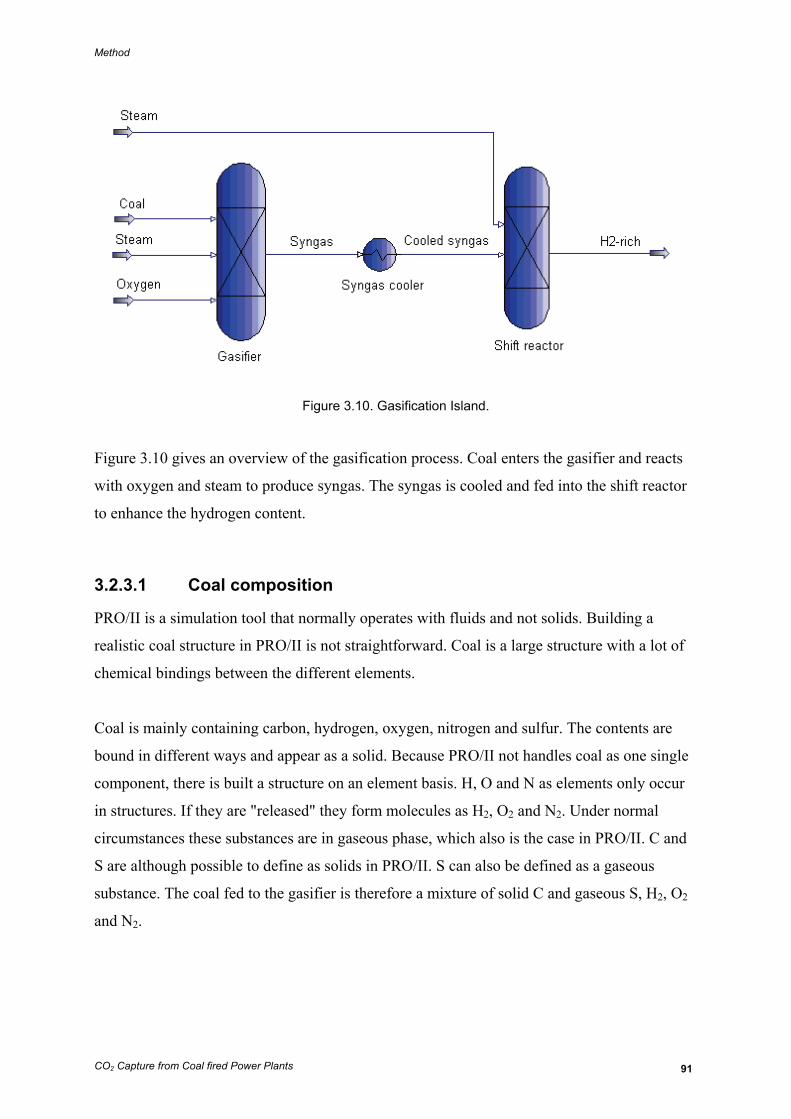
Method
CO2 Capture from Coal fired Power Plants 91
Figure 3.10. Gasification Island.
Figure 3.10 gives an overview of the gasification process. Coal enters the gasifier and reacts
with oxygen and steam to produce syngas. The syngas is cooled and fed into the shift reactor
to enhance the hydrogen content.
3.2.3.1 Coal composition
PRO/II is a simulation tool that normally operates with fluids and not solids. Building a
realistic coal structure in PRO/II is not straightforward. Coal is a large structure with a lot of
chemical bindings between the different elements.
Coal is mainly containing carbon, hydrogen, oxygen, nitrogen and sulfur. The contents are
bound in different ways and appear as a solid. Because PRO/II not handles coal as one single
component, there is built a structure on an element basis. H, O and N as elements only occur
in structures. If they are "released" they form molecules as H2, O2 and N2. Under normal
circumstances these substances are in gaseous phase, which also is the case in PRO/II. C and
S are although possible to define as solids in PRO/II. S can also be defined as a gaseous
substance. The coal fed to the gasifier is therefore a mixture of solid C and gaseous S, H2, O2
and N2.
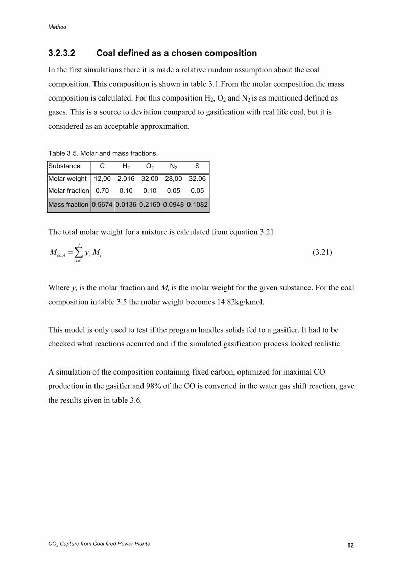
Method
CO2 Capture from Coal fired Power Plants 92
3.2.3.2 Coal defined as a chosen composition
In the first simulations there it is made a relative random assumption about the coal
composition. This composition is shown in table 3.1.From the molar composition the mass
composition is calculated. For this composition H2, O2 and N2 is as mentioned defined as
gases. This is a source to deviation compared to gasification with real life coal, but it is
considered as an acceptable approximation.
Table 3.5. Molar and mass fractions.
Substance C H2 O2 N2 S
Molar weight 12,00 2.016 32,00 28,00 32.06
Molar fraction 0.70 0.10 0.10 0.05 0.05
Mass fraction 0.5674 0.0136 0.2160 0.0948 0.1082
The total molar weight for a mixture is calculated from equation 3.21.
1
j
coal i ii
M y M=
=∑ (3.21)
Where yi is the molar fraction and Mi is the molar weight for the given substance. For the coal
composition in table 3.5 the molar weight becomes 14.82kg/kmol.
This model is only used to test if the program handles solids fed to a gasifier. It had to be
checked what reactions occurred and if the simulated gasification process looked realistic.
A simulation of the composition containing fixed carbon, optimized for maximal CO
production in the gasifier and 98% of the CO is converted in the water gas shift reaction, gave
the results given in table 3.6.
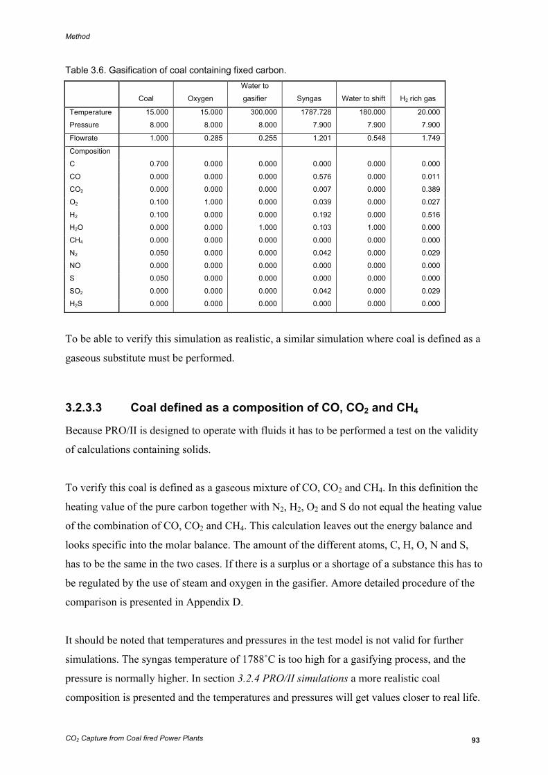
Method
CO2 Capture from Coal fired Power Plants 93
Table 3.6. Gasification of coal containing fixed carbon.
Coal Oxygen
Water to
gasifier Syngas Water to shift H2 rich gas
Temperature 15.000 15.000 300.000 1787.728 180.000 20.000
Pressure 8.000 8.000 8.000 7.900 7.900 7.900
Flowrate 1.000 0.285 0.255 1.201 0.548 1.749
Composition
C 0.700 0.000 0.000 0.000 0.000 0.000
CO 0.000 0.000 0.000 0.576 0.000 0.011
CO2 0.000 0.000 0.000 0.007 0.000 0.389
O2 0.100 1.000 0.000 0.039 0.000 0.027
H2 0.100 0.000 0.000 0.192 0.000 0.516
H2O 0.000 0.000 1.000 0.103 1.000 0.000
CH4 0.000 0.000 0.000 0.000 0.000 0.000
N2 0.050 0.000 0.000 0.042 0.000 0.029
NO 0.000 0.000 0.000 0.000 0.000 0.000
S 0.050 0.000 0.000 0.000 0.000 0.000
SO2 0.000 0.000 0.000 0.042 0.000 0.029
H2S 0.000 0.000 0.000 0.000 0.000 0.000
To be able to verify this simulation as realistic, a similar simulation where coal is defined as a
gaseous substitute must be performed.
3.2.3.3 Coal defined as a composition of CO, CO2 and CH4
Because PRO/II is designed to operate with fluids it has to be performed a test on the validity
of calculations containing solids.
To verify this coal is defined as a gaseous mixture of CO, CO2 and CH4. In this definition the
heating value of the pure carbon together with N2, H2, O2 and S do not equal the heating value
of the combination of CO, CO2 and CH4. This calculation leaves out the energy balance and
looks specific into the molar balance. The amount of the different atoms, C, H, O, N and S,
has to be the same in the two cases. If there is a surplus or a shortage of a substance this has to
be regulated by the use of steam and oxygen in the gasifier. Amore detailed procedure of the
comparison is presented in Appendix D.
It should be noted that temperatures and pressures in the test model is not valid for further
simulations. The syngas temperature of 1788˚C is too high for a gasifying process, and the
pressure is normally higher. In section 3.2.4 PRO/II simulations a more realistic coal
composition is presented and the temperatures and pressures will get values closer to real life.
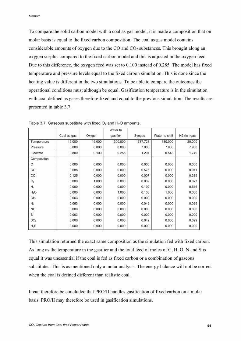
Method
CO2 Capture from Coal fired Power Plants 94
To compare the solid carbon model with a coal as gas model, it is made a composition that on
molar basis is equal to the fixed carbon composition. The coal as gas model contains
considerable amounts of oxygen due to the CO and CO2 substances. This brought along an
oxygen surplus compared to the fixed carbon model and this is adjusted in the oxygen feed.
Due to this difference, the oxygen feed was set to 0.100 instead of 0.285. The model has fixed
temperature and pressure levels equal to the fixed carbon simulation. This is done since the
heating value is different in the two simulations. To be able to compare the outcomes the
operational conditions must although be equal. Gasification temperature is in the simulation
with coal defined as gases therefore fixed and equal to the previous simulation. The results are
presented in table 3.7.
Table 3.7. Gaseous substitute with fixed O2 and H2O amounts.
Coal as gas Oxygen
Water to
gasifier Syngas Water to shift H2 rich gas
Temperature 15.000 15.000 300.000 1787.728 180.000 20.000
Pressure 8.000 8.000 8.000 7.900 7.900 7.900
Flowrate 0.800 0.100 0.255 1.201 0.548 1.749
Composition
C 0.000 0.000 0.000 0.000 0.000 0.000
CO 0.688 0.000 0.000 0.576 0.000 0.011
CO2 0.125 0.000 0.000 0.007 0.000 0.389
O2 0.000 1.000 0.000 0.039 0.000 0.027
H2 0.000 0.000 0.000 0.192 0.000 0.516
H2O 0.000 0.000 1.000 0.103 1.000 0.000
CH4 0.063 0.000 0.000 0.000 0.000 0.000
N2 0.063 0.000 0.000 0.042 0.000 0.029
NO 0.000 0.000 0.000 0.000 0.000 0.000
S 0.063 0.000 0.000 0.000 0.000 0.000
SO2 0.000 0.000 0.000 0.042 0.000 0.029
H2S 0.000 0.000 0.000 0.000 0.000 0.000
This simulation returned the exact same composition as the simulation fed with fixed carbon.
As long as the temperature in the gasifier and the total feed of moles of C, H, O, N and S is
equal it was unessential if the coal is fed as fixed carbon or a combination of gaseous
substitutes. This is as mentioned only a molar analysis. The energy balance will not be correct
when the coal is defined different than realistic coal.
It can therefore be concluded that PRO/II handles gasification of fixed carbon on a molar
basis. PRO/II may therefore be used in gasification simulations.
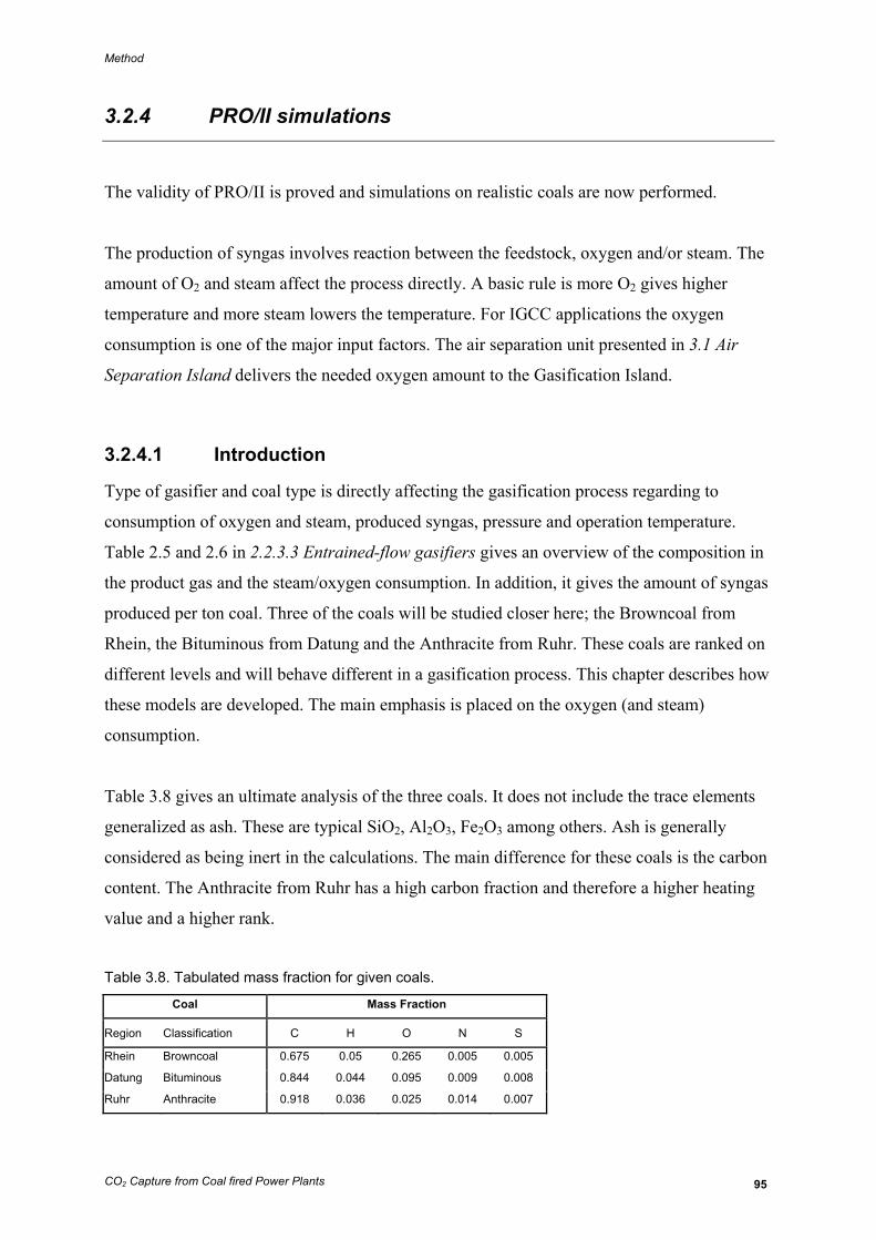
Method
CO2 Capture from Coal fired Power Plants 95
3.2.4 PRO/II simulations
The validity of PRO/II is proved and simulations on realistic coals are now performed.
The production of syngas involves reaction between the feedstock, oxygen and/or steam. The
amount of O2 and steam affect the process directly. A basic rule is more O2 gives higher
temperature and more steam lowers the temperature. For IGCC applications the oxygen
consumption is one of the major input factors. The air separation unit presented in 3.1 Air
Separation Island delivers the needed oxygen amount to the Gasification Island.
3.2.4.1 Introduction
Type of gasifier and coal type is directly affecting the gasification process regarding to
consumption of oxygen and steam, produced syngas, pressure and operation temperature.
Table 2.5 and 2.6 in 2.2.3.3 Entrained-flow gasifiers gives an overview of the composition in
the product gas and the steam/oxygen consumption. In addition, it gives the amount of syngas
produced per ton coal. Three of the coals will be studied closer here; the Browncoal from
Rhein, the Bituminous from Datung and the Anthracite from Ruhr. These coals are ranked on
different levels and will behave different in a gasification process. This chapter describes how
these models are developed. The main emphasis is placed on the oxygen (and steam)
consumption.
Table 3.8 gives an ultimate analysis of the three coals. It does not include the trace elements
generalized as ash. These are typical SiO2, Al2O3, Fe2O3 among others. Ash is generally
considered as being inert in the calculations. The main difference for these coals is the carbon
content. The Anthracite from Ruhr has a high carbon fraction and therefore a higher heating
value and a higher rank.
Table 3.8. Tabulated mass fraction for given coals.
Coal Mass Fraction
Region Classification C H O N S
Rhein Browncoal 0.675 0.05 0.265 0.005 0.005
Datung Bituminous 0.844 0.044 0.095 0.009 0.008
Ruhr Anthracite 0.918 0.036 0.025 0.014 0.007
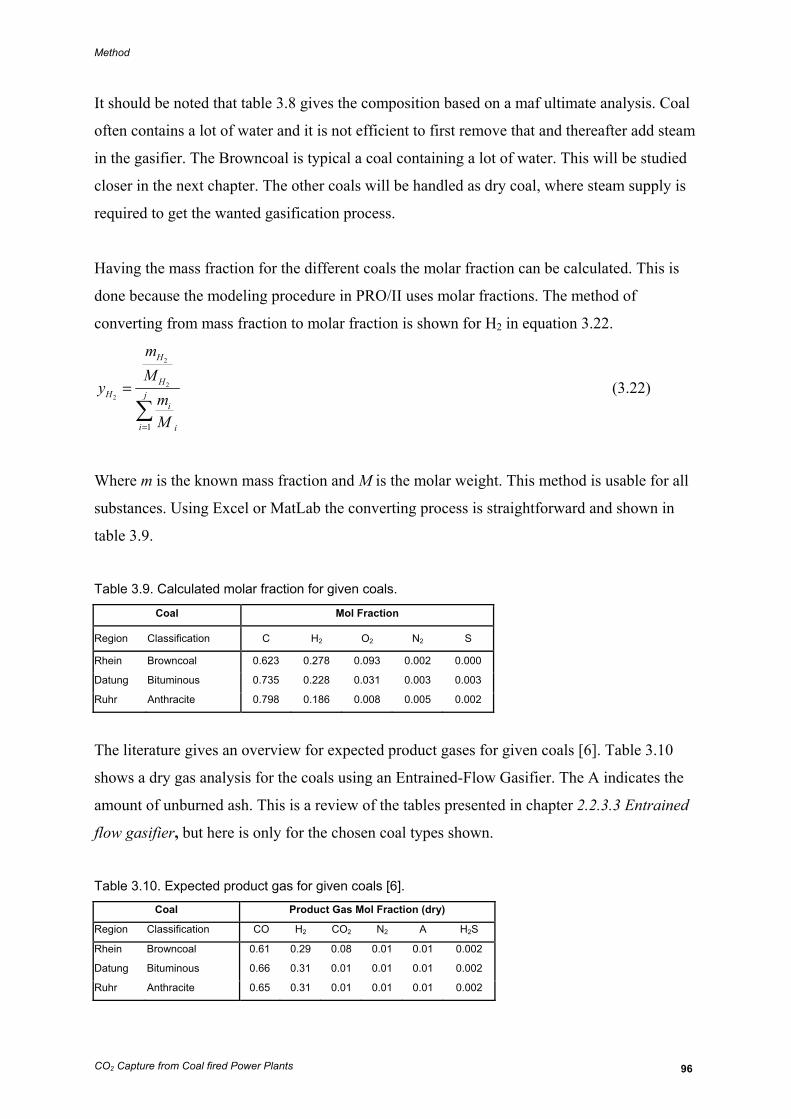
Method
CO2 Capture from Coal fired Power Plants 96
It should be noted that table 3.8 gives the composition based on a maf ultimate analysis. Coal
often contains a lot of water and it is not efficient to first remove that and thereafter add steam
in the gasifier. The Browncoal is typical a coal containing a lot of water. This will be studied
closer in the next chapter. The other coals will be handled as dry coal, where steam supply is
required to get the wanted gasification process.
Having the mass fraction for the different coals the molar fraction can be calculated. This is
done because the modeling procedure in PRO/II uses molar fractions. The method of
converting from mass fraction to molar fraction is shown for H2 in equation 3.22.
2
2
2
1
H
HH j
i
i i
mM
ymM=
=∑
(3.22)
Where m is the known mass fraction and M is the molar weight. This method is usable for all
substances. Using Excel or MatLab the converting process is straightforward and shown in
table 3.9.
Table 3.9. Calculated molar fraction for given coals.
Coal Mol Fraction
Region Classification C H2 O2 N2 S
Rhein Browncoal 0.623 0.278 0.093 0.002 0.000
Datung Bituminous 0.735 0.228 0.031 0.003 0.003
Ruhr Anthracite 0.798 0.186 0.008 0.005 0.002
The literature gives an overview for expected product gases for given coals [6]. Table 3.10
shows a dry gas analysis for the coals using an Entrained-Flow Gasifier. The A indicates the
amount of unburned ash. This is a review of the tables presented in chapter 2.2.3.3 Entrained
flow gasifier, but here is only for the chosen coal types shown.
Table 3.10. Expected product gas for given coals [6].
Coal Product Gas Mol Fraction (dry)
Region Classification CO H2 CO2 N2 A H2S
Rhein Browncoal 0.61 0.29 0.08 0.01 0.01 0.002
Datung Bituminous 0.66 0.31 0.01 0.01 0.01 0.002
Ruhr Anthracite 0.65 0.31 0.01 0.01 0.01 0.002
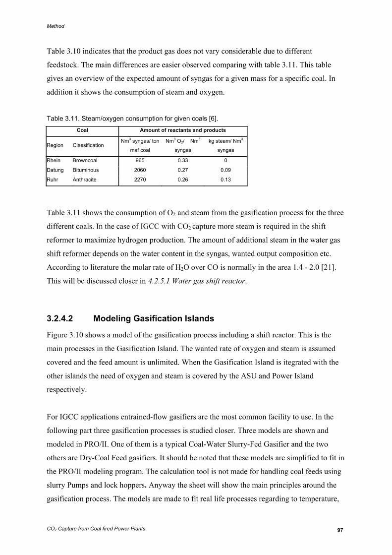
Method
CO2 Capture from Coal fired Power Plants 97
Table 3.10 indicates that the product gas does not vary considerable due to different
feedstock. The main differences are easier observed comparing with table 3.11. This table
gives an overview of the expected amount of syngas for a given mass for a specific coal. In
addition it shows the consumption of steam and oxygen.
Table 3.11. Steam/oxygen consumption for given coals [6].
Coal Amount of reactants and products
Region Classification Nm3 syngas/ ton
maf coal
Nm3 O2/ Nm3
syngas
kg steam/ Nm3
syngas
Rhein Browncoal 965 0.33 0
Datung Bituminous 2060 0.27 0.09
Ruhr Anthracite 2270 0.26 0.13
Table 3.11 shows the consumption of O2 and steam from the gasification process for the three
different coals. In the case of IGCC with CO2 capture more steam is required in the shift
reformer to maximize hydrogen production. The amount of additional steam in the water gas
shift reformer depends on the water content in the syngas, wanted output composition etc.
According to literature the molar rate of H2O over CO is normally in the area 1.4 - 2.0 [21].
This will be discussed closer in 4.2.5.1 Water gas shift reactor.
3.2.4.2 Modeling Gasification Islands
Figure 3.10 shows a model of the gasification process including a shift reactor. This is the
main processes in the Gasification Island. The wanted rate of oxygen and steam is assumed
covered and the feed amount is unlimited. When the Gasification Island is itegrated with the
other islands the need of oxygen and steam is covered by the ASU and Power Island
respectively.
For IGCC applications entrained-flow gasifiers are the most common facility to use. In the
following part three gasification processes is studied closer. Three models are shown and
modeled in PRO/II. One of them is a typical Coal-Water Slurry-Fed Gasifier and the two
others are Dry-Coal Feed gasifiers. It should be noted that these models are simplified to fit in
the PRO/II modeling program. The calculation tool is not made for handling coal feeds using
slurry Pumps and lock hoppers. Anyway the sheet will show the main principles around the
gasification process. The models are made to fit real life processes regarding to temperature,
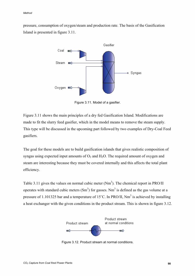
Method
CO2 Capture from Coal fired Power Plants 98
pressure, consumption of oxygen/steam and production rate. The basis of the Gasification
Island is presented in figure 3.11.
Figure 3.11. Model of a gasifier.
Figure 3.11 shows the main principles of a dry fed Gasification Island. Modifications are
made to fit the slurry feed gasifier, which in the model means to remove the steam supply.
This type will be discussed in the upcoming part followed by two examples of Dry-Coal Feed
gasifiers.
The goal for these models are to build gasification islands that gives realistic composition of
syngas using expected input amounts of O2 and H2O. The required amount of oxygen and
steam are interesting because they must be covered internally and this affects the total plant
efficiency.
Table 3.11 gives the values on normal cubic meter (Nm3). The chemical report in PRO/II
operates with standard cubic meters (Sm3) for gasses. Nm3 is defined as the gas volume at a
pressure of 1.101325 bar and a temperature of 15˚C. In PRO/II, Nm3 is achieved by installing
a heat exchanger with the given conditions in the product stream. This is shown in figure 3.12.
Figure 3.12. Product stream at normal conditions.
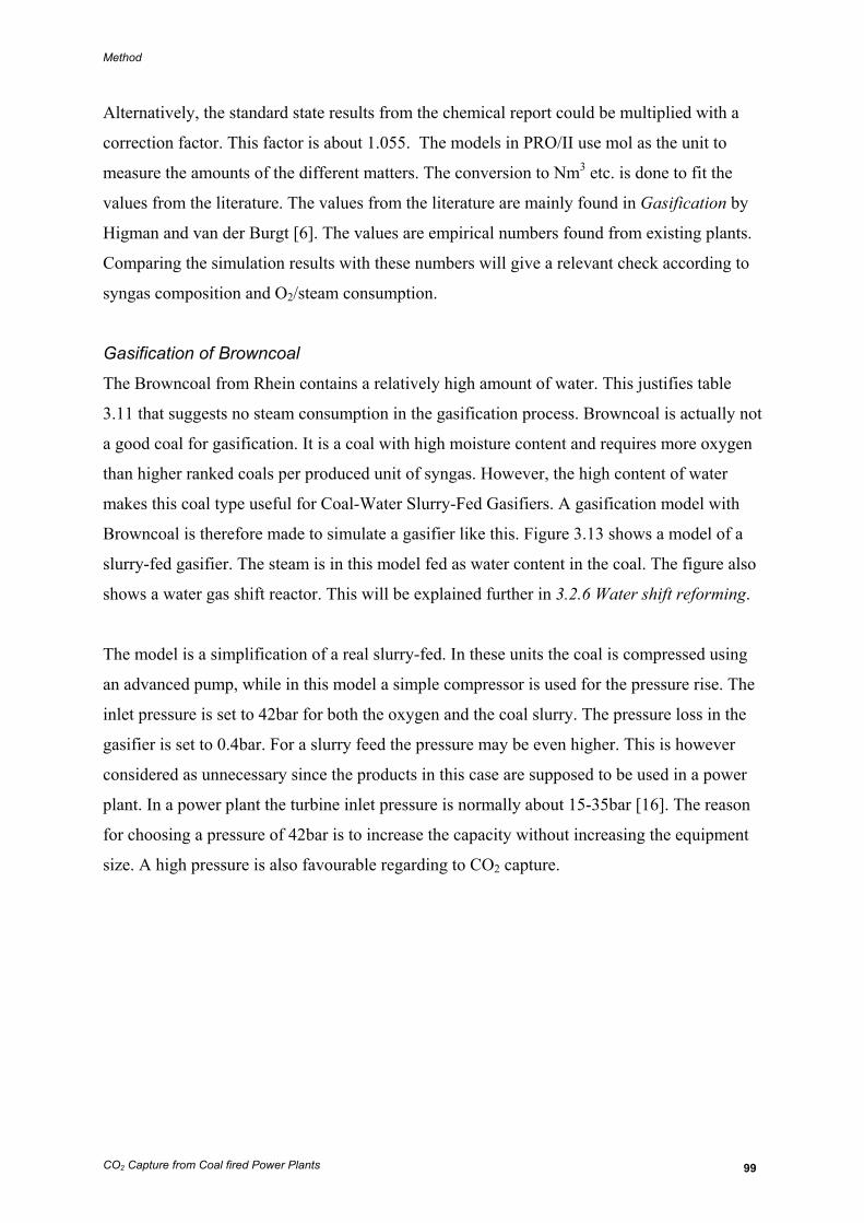
Method
CO2 Capture from Coal fired Power Plants 99
Alternatively, the standard state results from the chemical report could be multiplied with a
correction factor. This factor is about 1.055. The models in PRO/II use mol as the unit to
measure the amounts of the different matters. The conversion to Nm3 etc. is done to fit the
values from the literature. The values from the literature are mainly found in Gasification by
Higman and van der Burgt [6]. The values are empirical numbers found from existing plants.
Comparing the simulation results with these numbers will give a relevant check according to
syngas composition and O2/steam consumption.
Gasification of Browncoal
The Browncoal from Rhein contains a relatively high amount of water. This justifies table
3.11 that suggests no steam consumption in the gasification process. Browncoal is actually not
a good coal for gasification. It is a coal with high moisture content and requires more oxygen
than higher ranked coals per produced unit of syngas. However, the high content of water
makes this coal type useful for Coal-Water Slurry-Fed Gasifiers. A gasification model with
Browncoal is therefore made to simulate a gasifier like this. Figure 3.13 shows a model of a
slurry-fed gasifier. The steam is in this model fed as water content in the coal. The figure also
shows a water gas shift reactor. This will be explained further in 3.2.6 Water shift reforming.
The model is a simplification of a real slurry-fed. In these units the coal is compressed using
an advanced pump, while in this model a simple compressor is used for the pressure rise. The
inlet pressure is set to 42bar for both the oxygen and the coal slurry. The pressure loss in the
gasifier is set to 0.4bar. For a slurry feed the pressure may be even higher. This is however
considered as unnecessary since the products in this case are supposed to be used in a power
plant. In a power plant the turbine inlet pressure is normally about 15-35bar [16]. The reason
for choosing a pressure of 42bar is to increase the capacity without increasing the equipment
size. A high pressure is also favourable regarding to CO2 capture.
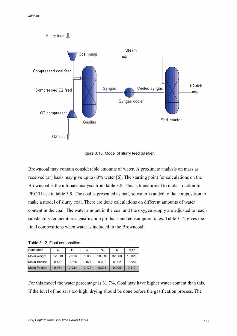
Method
CO2 Capture from Coal fired Power Plants 100
Figure 3.13. Model of slurry feed gasifier.
Browncoal may contain considerable amounts of water. A proximate analysis on mass as
received (ar) basis may give up to 60% water [6]. The starting point for calculations on the
Browncoal is the ultimate analysis from table 3.8. This is transformed to molar fraction for
PRO/II use in table 3.9. The coal is presented as maf, so water is added to the composition to
make a model of slurry coal. There are done calculations on different amounts of water
content in the coal. The water amount in the coal and the oxygen supply are adjusted to reach
satisfactory temperatures, gasification products and consumption rates. Table 3.12 gives the
final compositions when water is included in the Browncoal.
Table 3.12. Final composition.
Substance C H2 O2 N2 S H2O
Molar weight 12.010 2.016 32.000 28.010 32.060 18.020
Molar fraction 0.487 0.215 0.071 0.002 0.002 0.223
Mass fraction 0.461 0.034 0.179 0.004 0.005 0.317
For this model the water percentage is 31.7%. Coal may have higher water content than this.
If the level of moist is too high, drying should be done before the gasification process. The
Method
CO2 Capture from Coal fired Power Plants 101
drying process should occur naturally without external energy supply, for example by using
air.
The calculations around the gasification of Browncoal is shown and discussed in 4.2.3.1
Gasification of Browncoal.
Calculations on oxygen and steam consumption for Bituminous and Anthracite
Bituminous and Anthracite are high ranked coals which are suitable for gasification. The
oxygen consumption is relatively low. Typical values for this is presented in table 3.11.
A gasification model like the one shown in figure 3.11 is built to gasify coal types similar to
Bituminous and Anthracite, given in table 3.8 and 3.9. In this model the amount of coal and
the gasification pressure is defined as constant. 1kmol of coal is pressurized and fed to the
gasifier with a gasification pressure at 42bar. Pressurizing of coal is described in 2.2.3.5
Feeding procedures for a gasifier. In the model the feeding procedure is modeled as a
compressor. When the overall energy balance of a whole IGCC is calculated, there is added
an adjusted work for the feeding procedure. From literature the energy consumption for this is
suggested to be 11 MJ for 100 kg maf coal intake [6]. This is included in the overall
calculation in 4.5.1 Initial calculations.
The oxygen and steam are used as variables to reach a satisfactory composition of syngas. In
addition the gasification temperature must not exceed possible level for these facilities. A rule
of thumb says that more oxygen increases the temperature and more steam reduces the
temperature.
To make a relevant comparison, the production rate, the oxygen/steam consumption, the
syngas composition and the gasification temperature should not vary too much from the
values in table 3.10 and 3.11. These values are calculated doing iteration between the input
factors.
The first step is to find a production rate, which means amount of Nm3 syngas per ton of maf
coal. This number is expected to vary from the literature since the gasification model deals
with coal as a composition of five elements and not a complete material. A heat exchanger is,
Method
CO2 Capture from Coal fired Power Plants 102
similar to figure 3.12, implemented in the model to get normal conditions. The Bituminous
coal with given molar/mass fractions has for example a molecular weight of 10.45kg/kmol.
Since the model operates with a coal feed of 1kmol the feed rate has the same value,
10.45kg/s. This numbers may be calculated, but in PRO/II it can be red directly from a
chemical report. The amount of syngas is found by adding the molar fractions of CO and H2
and multiply the numbers with the normalized amount of syngas. When the volume of syngas
and the weight of the coal are known, the ratio Nm3 syngas/ton coal can be set up. The values
are comparable with the values found in literature.
The next step is to get the right amounts of oxygen and steam. The oxygen to syngas rate
could be calculated directly from the chemical report at standard conditions since the
correlation between Nm3 and Sm3 is the same for both gasses. The amount of oxygen is
regulated to reach a close to real life rate, but not exceeding a realistic gasification
temperature. A too high gasification temperature could be regulated with steam, but also here
there are limits. Too much steam will cause too high water content in the product gas. The
steam consumption is in literature calculated as kg steam/ Nm3 syngas. The chemical report
gives the rate on mass basis and the amount of syngas at normal state is found using the same
method as mentioned earlier. The same number could not be used since the change in input
regarding to oxygen and steam also contributes to a change in the amount of syngas and in the
composition.
These operations are repeated until acceptable levels of oxygen, steam, syngas composition
and temperature are reached. The numbers are shown and discussed in chapter 4.2.3 PRO/II
simulations.
3.2.5 Chemical equilibrium calculator
In addition to PRO/II calculations there are done some direct calculations using an online
chemical equilibrium calculator. The chemical equilibrium calculator gives the molar and
mass fractions for given reactants at given temperatures and pressure. It is a tool where the
users define two constant constraints among pressure, volume, temperature, entropy, enthalpy
and internal energy. In this case constant volume and constant pressure are assumed. This is
because in a gasifier the volume is fixed by the control volume. Constant pressure is also valid

Method
CO2 Capture from Coal fired Power Plants 103
since the reactants all are fed at the gasification pressure. There is be pressure loss in the
gasification reaction, as in all other reactions, but this can be consider it as negligible for
chemical equilibrium calculation purposes. The temperature is calculated using two initial
values. The calculator names them starting temperature and estimated equilibrium
temperature. The chemical equilibrium calculator handles coal in the same way as PRO/II,
which means that the coal is defined as a mixture of C, H2, O2, S and N2. The calculator also
handles pure elements like H instead of H2. It is therefore done calculations on both atomic
and molecular level. On an atomic level the molar fraction differ since the molar weight is
halved for the hydrogen, oxygen and nitrogen. Table 3.13 gives the fractions for this special
case.
Table 3.13. Coal types on elementary basis.
Coal Mol Fraction
Region Classification C H O N S H2O
Rhein Browncoal 0.471 0.387 0.137 0.003 0.002 0.000
Rhein with water 0,387 0.318 0.113 0.003 0.002 0.178
Datung Bituminous 0.596 0.346 0.050 0.005 0.002 0.000
Ruhr Anthracite 0.683 0.296 0.014 0.009 0.002 0.000
Molar fractions of the coal, H2O and pure O2 are given to the calculator and set to the same
gasification pressure as in PRO/II. The gasification temperature is calculated in the program,
and therefore some trial and failure among initial temperature and estimated equilibrium
temperature is done to reach the same temperature as in the other model.
3.2.6 Water shift reforming
3.2.6.1 Water gas shift reactor
The procedure after the gasification is independent of the coal feed. The product gas contains
much the same fractions of CO and H2. In further calculation it is only focused on one coal.
The principles are though the same for all the coals, with some minor modifications. The
Bituminous coal from Datung, China, is studied through the rest of the calculations. This is a
good coal for gasification and there are available literature about composition and heating
values.
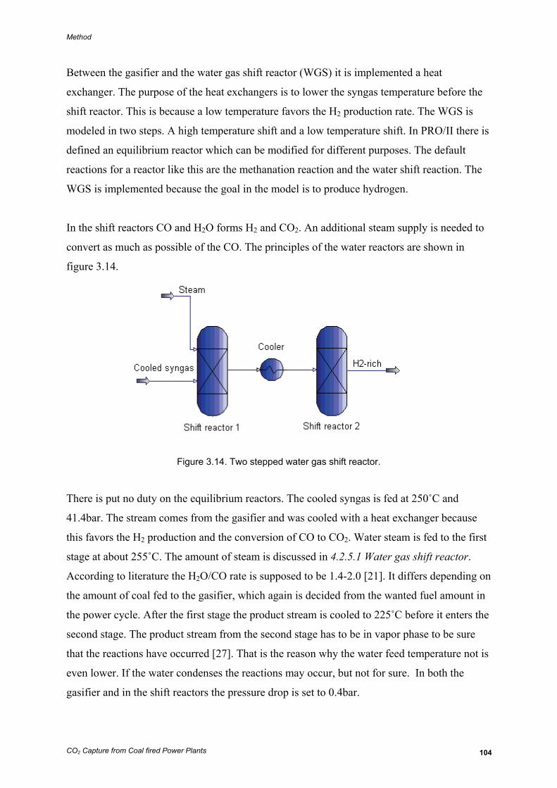
Method
CO2 Capture from Coal fired Power Plants 104
Between the gasifier and the water gas shift reactor (WGS) it is implemented a heat
exchanger. The purpose of the heat exchangers is to lower the syngas temperature before the
shift reactor. This is because a low temperature favors the H2 production rate. The WGS is
modeled in two steps. A high temperature shift and a low temperature shift. In PRO/II there is
defined an equilibrium reactor which can be modified for different purposes. The default
reactions for a reactor like this are the methanation reaction and the water shift reaction. The
WGS is implemented because the goal in the model is to produce hydrogen.
In the shift reactors CO and H2O forms H2 and CO2. An additional steam supply is needed to
convert as much as possible of the CO. The principles of the water reactors are shown in
figure 3.14.
Figure 3.14. Two stepped water gas shift reactor.
There is put no duty on the equilibrium reactors. The cooled syngas is fed at 250˚C and
41.4bar. The stream comes from the gasifier and was cooled with a heat exchanger because
this favors the H2 production and the conversion of CO to CO2. Water steam is fed to the first
stage at about 255˚C. The amount of steam is discussed in 4.2.5.1 Water gas shift reactor.
According to literature the H2O/CO rate is supposed to be 1.4-2.0 [21]. It differs depending on
the amount of coal fed to the gasifier, which again is decided from the wanted fuel amount in
the power cycle. After the first stage the product stream is cooled to 225˚C before it enters the
second stage. The product stream from the second stage has to be in vapor phase to be sure
that the reactions have occurred [27]. That is the reason why the water feed temperature not is
even lower. If the water condenses the reactions may occur, but not for sure. In both the
gasifier and in the shift reactors the pressure drop is set to 0.4bar.
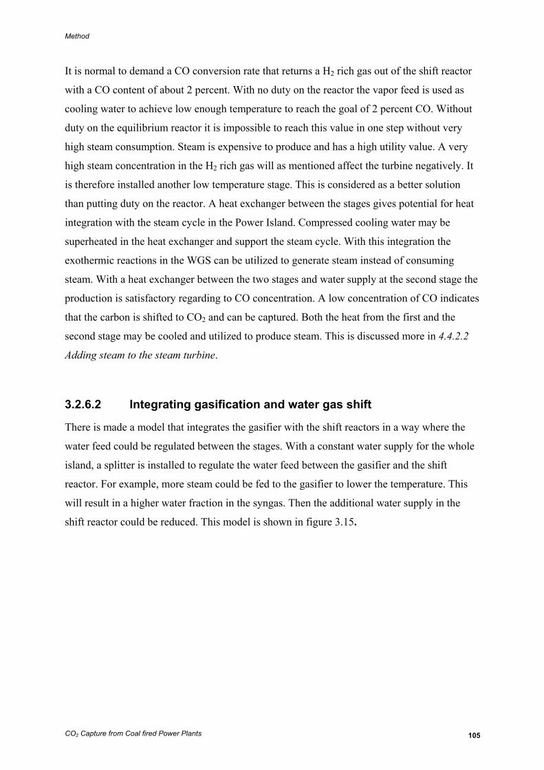
Method
CO2 Capture from Coal fired Power Plants 105
It is normal to demand a CO conversion rate that returns a H2 rich gas out of the shift reactor
with a CO content of about 2 percent. With no duty on the reactor the vapor feed is used as
cooling water to achieve low enough temperature to reach the goal of 2 percent CO. Without
duty on the equilibrium reactor it is impossible to reach this value in one step without very
high steam consumption. Steam is expensive to produce and has a high utility value. A very
high steam concentration in the H2 rich gas will as mentioned affect the turbine negatively. It
is therefore installed another low temperature stage. This is considered as a better solution
than putting duty on the reactor. A heat exchanger between the stages gives potential for heat
integration with the steam cycle in the Power Island. Compressed cooling water may be
superheated in the heat exchanger and support the steam cycle. With this integration the
exothermic reactions in the WGS can be utilized to generate steam instead of consuming
steam. With a heat exchanger between the two stages and water supply at the second stage the
production is satisfactory regarding to CO concentration. A low concentration of CO indicates
that the carbon is shifted to CO2 and can be captured. Both the heat from the first and the
second stage may be cooled and utilized to produce steam. This is discussed more in 4.4.2.2
Adding steam to the steam turbine.
3.2.6.2 Integrating gasification and water gas shift
There is made a model that integrates the gasifier with the shift reactors in a way where the
water feed could be regulated between the stages. With a constant water supply for the whole
island, a splitter is installed to regulate the water feed between the gasifier and the shift
reactor. For example, more steam could be fed to the gasifier to lower the temperature. This
will result in a higher water fraction in the syngas. Then the additional water supply in the
shift reactor could be reduced. This model is shown in figure 3.15.
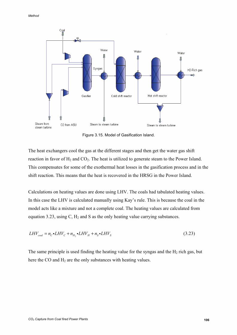
Method
CO2 Capture from Coal fired Power Plants 106
Figure 3.15. Model of Gasification Island.
The heat exchangers cool the gas at the different stages and then get the water gas shift
reaction in favor of H2 and CO2. The heat is utilized to generate steam to the Power Island.
This compensates for some of the exothermal heat losses in the gasification process and in the
shift reaction. This means that the heat is recovered in the HRSG in the Power Island.
Calculations on heating values are done using LHV. The coals had tabulated heating values.
In this case the LHV is calculated manually using Kay’s rule. This is because the coal in the
model acts like a mixture and not a complete coal. The heating values are calculated from
equation 3.23, using C, H2 and S as the only heating value carrying substances.
2coal C C H H S SLHV n LHV n LHV n LHV= + +i i i (3.23)
The same principle is used finding the heating value for the syngas and the H2 rich gas, but
here the CO and H2 are the only substances with heating values.
Method
CO2 Capture from Coal fired Power Plants 107
3.3 Acid Gas Removal
3.3.1 Simulation tool
There are not performed any simulations on an acid gas remover. To calculate the energy
demand of the island, capture costs based on energy consumption per captured amount of
carbon dioxide is used. The calculations are done in Microsoft Excel.
Stream properties out of the AGR unit are also calculated in Microsoft Excel. The fuel
composition into the unit is calculated in 3.2 Gasification Island and with a capture efficiency
presented in the subsequent section the cleaned fuel stream is found.
3.3.2 CO2 capture unit
When choosing a CO2 capture process, the partial pressure of carbon dioxide and the scale of
the plant are important decision factors. An IGCC plant is in most occasions considered as
large scale plants and the capture process chosen need to handle large amounts of CO2. The
fuel gas from the water gas shift reactor contains mainly hydrogen and carbon dioxide. The
distribution is on dry basis 58.2% H2, 39.0% CO2, 2.4% CO, 0.2% N2 and 0.1% H2S. The
pressure after the shift reactor is at 40.2bar. This gives a partial pressure of carbon dioxide of
about 15.7bar which is considered as high.
On behalf of the large scale of the plant and the high CO2 partial pressure it is decided to use
an absorber in the capture process. Because of the relatively high pressure in the fuel stream
physical absorption is preferred before chemical absorption [21].
In this report there are not done any simulations or tests on the CO2 capture unit. A capture
method is chosen and energy consumption per kilogram captured carbon dioxide is used to
calculate plant efficiency reduction and unit energy consumption.
Method
CO2 Capture from Coal fired Power Plants 108
The gasifier chosen in 3.2 Gasification Island is an entrained flow gasifier. The most common
entrained flow gasifier is the shell gasifier. The gas from a shell gasifier performs desirable
with selexol used as solvent in a physical absorption process. The following key numbers are
therefore used in further calculations on the acid gas remover.
Table 3.14. Properties of the Acid Gas Remover [21].
Gasification method Shell CO2 capture technology Physical absorption CO2/H2 separation method Selexol CO2 capture ratio 96 % CO2 scrubbing cost 0.06-0.11 kWh/kg CO2 captured CO2 compression cost 0.11-0.13 kWh/kg CO2 captured
The total amount of captured carbon dioxide must be found to calculate the total energy
consumption in the acid gas remover. This is done in the calculations of the entire IGCC
plant.
The scrubbing cost presented in table 3.14 is mainly the cost of pressurize the solvent to fuel
gas pressure. The solvent is sent to the fuel gas and the CO2 is absorbed to the selexol. Selexol
with attached carbon dioxide is then removed from the fuel gas. The separation of selexol and
CO2 is done by expansion to atmospheric pressure. Then the selexol is regenerated and the
carbon dioxide must be compressed to a desirable storage pressure. The compression cost of a
pressure rise to 110bar is given in table 3.14. This energy demand must be implemented in the
total energy cost calculation of CO2 capture.
The capture ratio of CO2 is also given in table 3.14. 96% of the carbon dioxide is led out of
the black box in a separate stream. The remaining CO2 is sent to the turbine together with H2
and the other substances in the fuel gas. As an end product with no heating value, the carbon
dioxide is inert and do not react in the combustion chamber. The remaining 4% of the CO2 is
therefore emitted to the environment.
Figure 3.16 in 3.3.2 H2S capture unit is showing a black box overview and table 3.15 is
giving the stream properties.
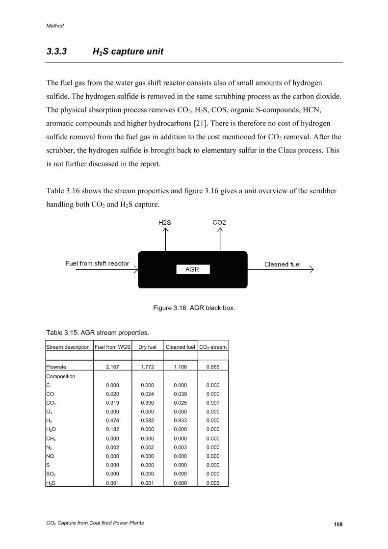
Method
CO2 Capture from Coal fired Power Plants 109
3.3.3 H2S capture unit
The fuel gas from the water gas shift reactor consists also of small amounts of hydrogen
sulfide. The hydrogen sulfide is removed in the same scrubbing process as the carbon dioxide.
The physical absorption process removes CO2, H2S, COS, organic S-compounds, HCN,
aromatic compounds and higher hydrocarbons [21]. There is therefore no cost of hydrogen
sulfide removal from the fuel gas in addition to the cost mentioned for CO2 removal. After the
scrubber, the hydrogen sulfide is brought back to elementary sulfur in the Claus process. This
is not further discussed in the report.
Table 3.16 shows the stream properties and figure 3.16 gives a unit overview of the scrubber
handling both CO2 and H2S capture.
Figure 3.16. AGR black box.
Table 3.15. AGR stream properties.
Stream description Fuel from WGS Dry fuel Cleaned fuel CO2-stream
Flowrate 2.167 1.772 1.106 0.666
Composition
C 0.000 0.000 0.000 0.000
CO 0.020 0.024 0.039 0.000
CO2 0.319 0.390 0.025 0.997
O2 0.000 0.000 0.000 0.000
H2 0.476 0.582 0.933 0.000
H2O 0.182 0.000 0.000 0.000
CH4 0.000 0.000 0.000 0.000
N2 0.002 0.002 0.003 0.000
NO 0.000 0.000 0.000 0.000
S 0.000 0.000 0.000 0.000
SO2 0.000 0.000 0.000 0.000
H2S 0.001 0.001 0.000 0.003

Method
CO2 Capture from Coal fired Power Plants 110
It is assumed no leakage of H2 or other substances in the CO2 and H2S stream. In a real plant
there will probably be some minor amounts of the other substances in the waste streams
reducing the fuel stream.
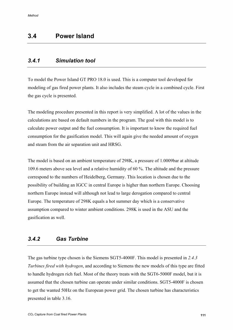
Method
CO2 Capture from Coal fired Power Plants 111
3.4 Power Island
3.4.1 Simulation tool
To model the Power Island GT PRO 18.0 is used. This is a computer tool developed for
modeling of gas fired power plants. It also includes the steam cycle in a combined cycle. First
the gas cycle is presented.
The modeling procedure presented in this report is very simplified. A lot of the values in the
calculations are based on default numbers in the program. The goal with this model is to
calculate power output and the fuel consumption. It is important to know the required fuel
consumption for the gasification model. This will again give the needed amount of oxygen
and steam from the air separation unit and HRSG.
The model is based on an ambient temperature of 298K, a pressure of 1.0009bar at altitude
109.6 meters above sea level and a relative humidity of 60 %. The altitude and the pressure
correspond to the numbers of Heidelberg, Germany. This location is chosen due to the
possibility of building an IGCC in central Europe is higher than northern Europe. Choosing
northern Europe instead will although not lead to large derogation compared to central
Europe. The temperature of 298K equals a hot summer day which is a conservative
assumption compared to winter ambient conditions. 298K is used in the ASU and the
gasification as well.
3.4.2 Gas Turbine
The gas turbine type chosen is the Siemens SGT5-4000F. This model is presented in 2.4.3
Turbines fired with hydrogen, and according to Siemens the new models of this type are fitted
to handle hydrogen rich fuel. Most of the theory treats with the SGT6-5000F model, but it is
assumed that the chosen turbine can operate under similar conditions. SGT5-4000F is chosen
to get the wanted 50Hz on the European power grid. The chosen turbine has characteristics
presented in table 3.16.
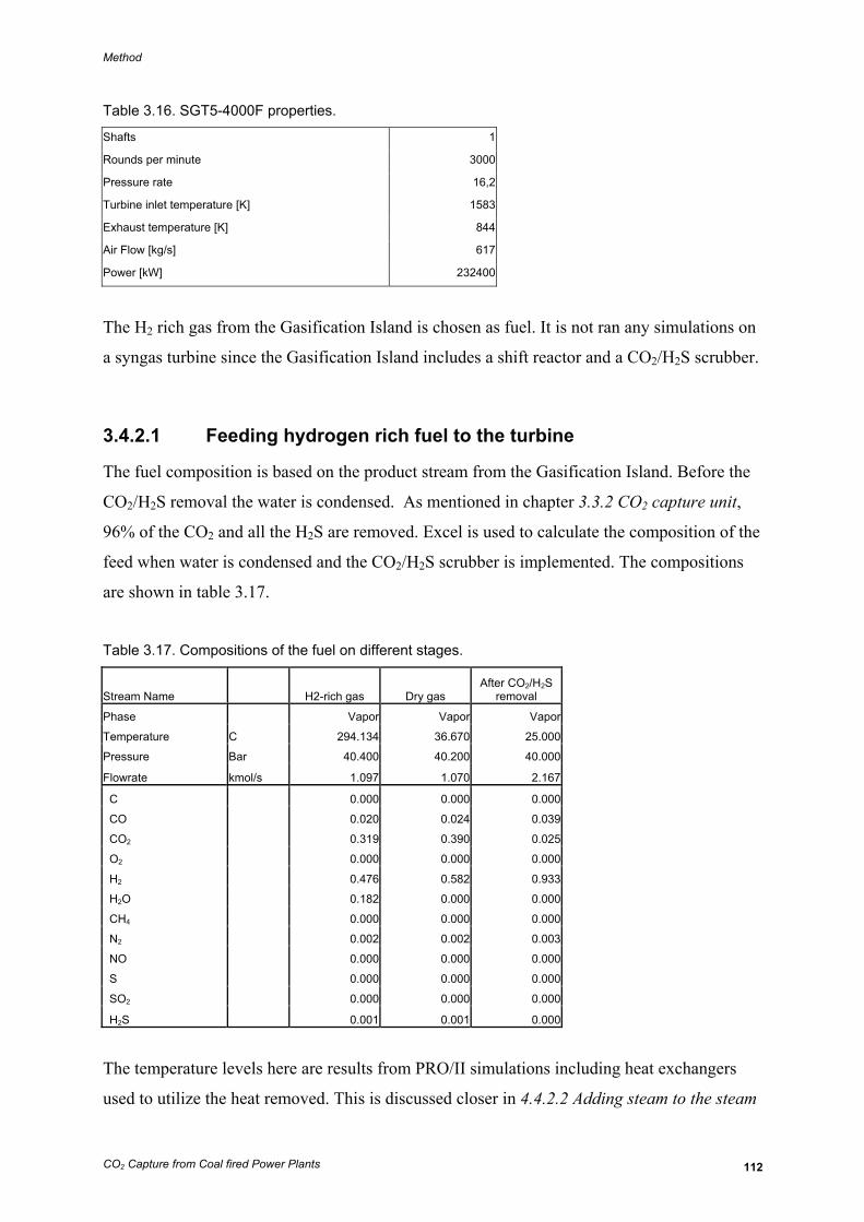
Method
CO2 Capture from Coal fired Power Plants 112
Table 3.16. SGT5-4000F properties. Shafts 1
Rounds per minute 3000
Pressure rate 16,2
Turbine inlet temperature [K] 1583
Exhaust temperature [K] 844
Air Flow [kg/s] 617
Power [kW] 232400
The H2 rich gas from the Gasification Island is chosen as fuel. It is not ran any simulations on
a syngas turbine since the Gasification Island includes a shift reactor and a CO2/H2S scrubber.
3.4.2.1 Feeding hydrogen rich fuel to the turbine
The fuel composition is based on the product stream from the Gasification Island. Before the
CO2/H2S removal the water is condensed. As mentioned in chapter 3.3.2 CO2 capture unit,
96% of the CO2 and all the H2S are removed. Excel is used to calculate the composition of the
feed when water is condensed and the CO2/H2S scrubber is implemented. The compositions
are shown in table 3.17.
Table 3.17. Compositions of the fuel on different stages.
Stream Name H2-rich gas Dry gas After CO2/H2S
removal
Phase Vapor Vapor Vapor
Temperature C 294.134 36.670 25.000
Pressure Bar 40.400 40.200 40.000
Flowrate kmol/s 1.097 1.070 2.167
C 0.000 0.000 0.000
CO 0.020 0.024 0.039
CO2 0.319 0.390 0.025
O2 0.000 0.000 0.000
H2 0.476 0.582 0.933
H2O 0.182 0.000 0.000
CH4 0.000 0.000 0.000
N2 0.002 0.002 0.003
NO 0.000 0.000 0.000
S 0.000 0.000 0.000
SO2 0.000 0.000 0.000
H2S 0.001 0.001 0.000
The temperature levels here are results from PRO/II simulations including heat exchangers
used to utilize the heat removed. This is discussed closer in 4.4.2.2 Adding steam to the steam
Method
CO2 Capture from Coal fired Power Plants 113
turbine. There is still some CO2 in the mass flow. The carbon dioxide act as an inert and
increase the mass flow through the turbine. So for the power production it is not negative, but
it will lead to a small CO2 emission. The CO contains heating value and is converted to CO2
in the combustion process. Because of the very high fraction of H2 the fuel stream is diluted
with nitrogen from the Air Separation Island.
In ordinary gas turbines water steam can be utilized as a diluter. For hydrogen turbines this is
not the case. It contributes to higher moisture in the turbine that again affects the heat transfer
and put more strain on the materials. When also CO2 capture is included the water removal
contributes to a higher fraction of CO2 before the removing process.
Table 2.7 in 2.4.3 Turbines fired with hydrogen shows that the chosen turbine can handle a
hydrogen fraction at 70 % and even higher. It is therefore run a simulation with 70 % H2 with
N2 used as an extra diluter in addition to the small CO2 amounts. That gave a relatively low
demand of nitrogen. Nitrogen is available from the ASU. The ASU produces the required
amount of oxygen for the gasification process and this gives a considerable amount of N2. It is
therefore beneficial to consume this nitrogen in the turbine to increase the mass flow and
regulate the temperature. GTPRO gives the required mass fraction for each fuel composition.
The wanted amount of hydrogen can then be calculated. When the required amount of
hydrogen is calculated, the necessary amount of oxygen for the given coal in the given
gasifier is found. That amount of O2 will again give the amount of N2 that is produced for the
given amount of O2 in the ASU.
The 70% H2 fuel gave a considerable lower N2 demand than the appurtenant production of N2
in the ASU based on the O2 demand for the gasification. The N2 amount is therefore
increased. When increasing the N2 amount in the fuel flow it is important to keep the same
scale between the other substances so the overall mass balance is correct. This is done in
Excel. Several iterations are performed to get a suitable amount of hydrogen and nitrogen that
corresponded to the O2/N2 production in the ASU. The final composition of fuel diluted with
N2 is shown in table 3.18.
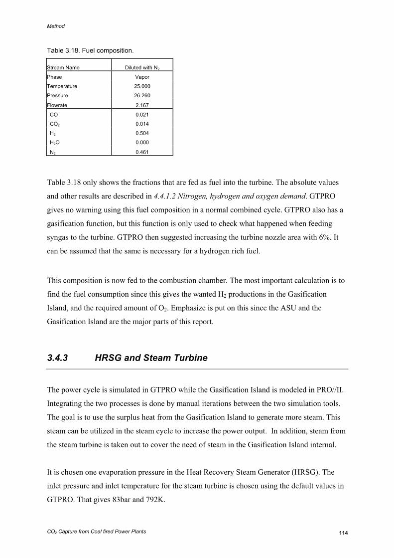
Method
CO2 Capture from Coal fired Power Plants 114
Table 3.18. Fuel composition.
Stream Name Diluted with N2
Phase Vapor
Temperature 25.000
Pressure 26.260
Flowrate 2.167
CO 0.021
CO2 0.014
H2 0.504
H2O 0.000
N2 0.461
Table 3.18 only shows the fractions that are fed as fuel into the turbine. The absolute values
and other results are described in 4.4.1.2 Nitrogen, hydrogen and oxygen demand. GTPRO
gives no warning using this fuel composition in a normal combined cycle. GTPRO also has a
gasification function, but this function is only used to check what happened when feeding
syngas to the turbine. GTPRO then suggested increasing the turbine nozzle area with 6%. It
can be assumed that the same is necessary for a hydrogen rich fuel.
This composition is now fed to the combustion chamber. The most important calculation is to
find the fuel consumption since this gives the wanted H2 productions in the Gasification
Island, and the required amount of O2. Emphasize is put on this since the ASU and the
Gasification Island are the major parts of this report.
3.4.3 HRSG and Steam Turbine
The power cycle is simulated in GTPRO while the Gasification Island is modeled in PRO//II.
Integrating the two processes is done by manual iterations between the two simulation tools.
The goal is to use the surplus heat from the Gasification Island to generate more steam. This
steam can be utilized in the steam cycle to increase the power output. In addition, steam from
the steam turbine is taken out to cover the need of steam in the Gasification Island internal.
It is chosen one evaporation pressure in the Heat Recovery Steam Generator (HRSG). The
inlet pressure and inlet temperature for the steam turbine is chosen using the default values in
GTPRO. That gives 83bar and 792K.
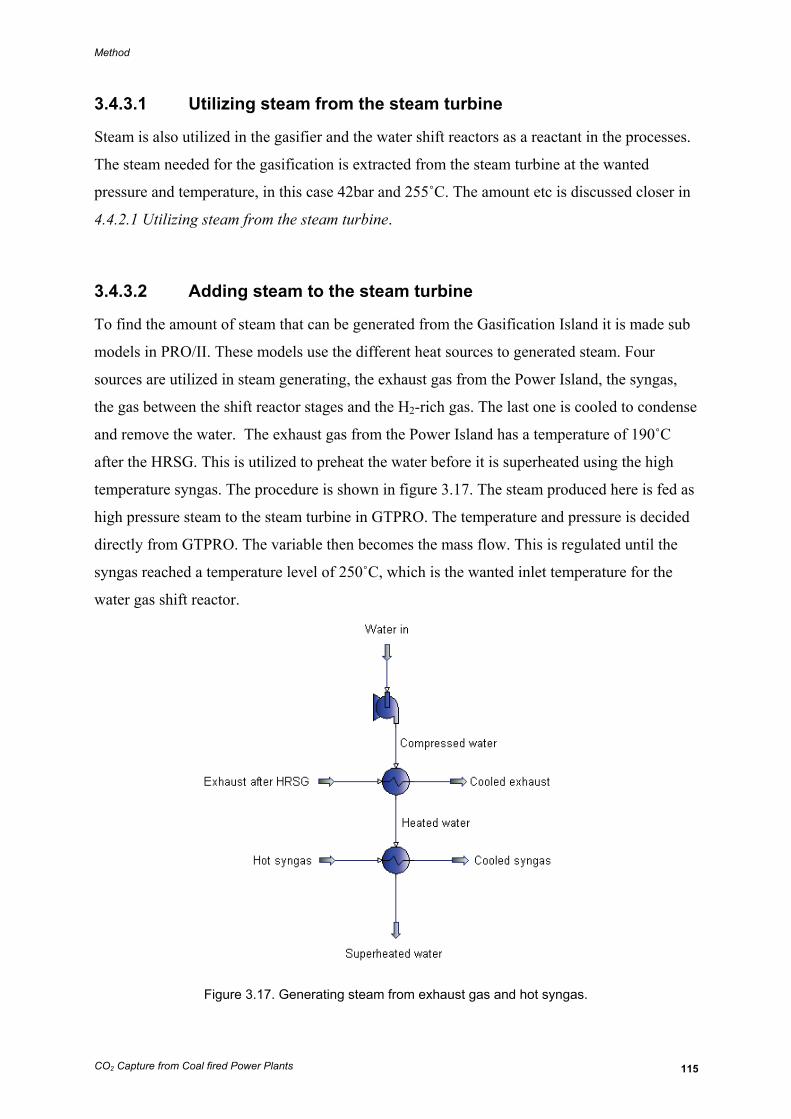
Method
CO2 Capture from Coal fired Power Plants 115
3.4.3.1 Utilizing steam from the steam turbine
Steam is also utilized in the gasifier and the water shift reactors as a reactant in the processes.
The steam needed for the gasification is extracted from the steam turbine at the wanted
pressure and temperature, in this case 42bar and 255˚C. The amount etc is discussed closer in
4.4.2.1 Utilizing steam from the steam turbine.
3.4.3.2 Adding steam to the steam turbine
To find the amount of steam that can be generated from the Gasification Island it is made sub
models in PRO/II. These models use the different heat sources to generated steam. Four
sources are utilized in steam generating, the exhaust gas from the Power Island, the syngas,
the gas between the shift reactor stages and the H2-rich gas. The last one is cooled to condense
and remove the water. The exhaust gas from the Power Island has a temperature of 190˚C
after the HRSG. This is utilized to preheat the water before it is superheated using the high
temperature syngas. The procedure is shown in figure 3.17. The steam produced here is fed as
high pressure steam to the steam turbine in GTPRO. The temperature and pressure is decided
directly from GTPRO. The variable then becomes the mass flow. This is regulated until the
syngas reached a temperature level of 250˚C, which is the wanted inlet temperature for the
water gas shift reactor.
Figure 3.17. Generating steam from exhaust gas and hot syngas.
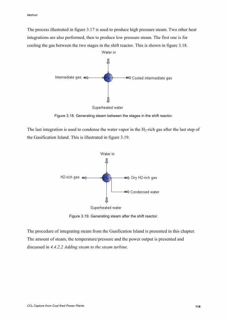
Method
CO2 Capture from Coal fired Power Plants 116
The process illustrated in figure 3.17 is used to produce high pressure steam. Two other heat
integrations are also performed, then to produce low pressure steam. The first one is for
cooling the gas between the two stages in the shift reactor. This is shown in figure 3.18.
Figure 3.18. Generating steam between the stages in the shift reactor.
The last integration is used to condense the water vapor in the H2-rich gas after the last step of
the Gasification Island. This is illustrated in figure 3.19.
Figure 3.19. Generating steam after the shift reactor.
The procedure of integrating steam from the Gasification Island is presented in this chapter.
The amount of steam, the temperature/pressure and the power output is presented and
discussed in 4.4.2.2 Adding steam to the steam turbine.
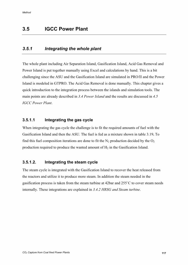
Method
CO2 Capture from Coal fired Power Plants 117
3.5 IGCC Power Plant
3.5.1 Integrating the whole plant
The whole plant including Air Separation Island, Gasification Island, Acid Gas Removal and
Power Island is put together manually using Excel and calculations by hand. This is a bit
challenging since the ASU and the Gasification Island are simulated in PRO/II and the Power
Island is modeled in GTPRO. The Acid Gas Removal is done manually. This chapter gives a
quick introduction to the integration process between the islands and simulation tools. The
main points are already described in 3.4 Power Island and the results are discussed in 4.5
IGCC Power Plant.
3.5.1.1 Integrating the gas cycle
When integrating the gas cycle the challenge is to fit the required amounts of fuel with the
Gasification Island and then the ASU. The fuel is fed as a mixture shown in table 3.19. To
find this fuel composition iterations are done to fit the N2 production decided by the O2
production required to produce the wanted amount of H2 in the Gasification Island.
3.5.1.2. Integrating the steam cycle
The steam cycle is integrated with the Gasification Island to recover the heat released from
the reactors and utilize it to produce more steam. In addition the steam needed in the
gasification process is taken from the steam turbine at 42bar and 255˚C to cover steam needs
internally. These integrations are explained in 3.4.2 HRSG and Steam turbine.
Results and Discussion
CO2 Capture from Coal fired Power Plants 118
4 Results and Discussion
4.1 Air Separation Island
4.1.1 Gaseous oxygen
In this part of the report, results achieved in the PRO/II models presented in 3.1. Air
Separation Island are discussed. The results of the GOX plant are first analyzed and
optimized. Variations and sensitivity are discussed. Afterwards the produced oxygen is
compressed to compare the GOX and LOX plant.
4.1.1.1 Energy consumption considerations
A figure of the initial developed GOX plant is shown in figure 3.8 in 3.1.2.8 After treatment
of oxygen and nitrogen. Stream properties for all the streams in the model are given in
Appendix E.
The only work added to the island is the compressor work of the four compressors forming
the main air compressor. The properties of the compressors are given in table 3.2 first shown
in 3.1.2.2 Air cleaning.
Table 3.2. Compressor work of compressing 0.99 kmol of dry air. Compressor Name C1 C2 C3 C4
Pressure bar 1.60 2.50 4.00 6.43
Temperature K 348.94 348.39 351.33 351.91
Head m 5224 5167 5468 5526
Actual Work kW 1469 1453 1538 1554
Isentropic coef.. k 1.4013 1.4024 1.4041 1.407
By adding the compressor work from the compressors it is found that the total work is
6014kW. The optimal distribution of work is from theory achieved when the compressors
Results and Discussion
CO2 Capture from Coal fired Power Plants 119
have equal work. It is although found that the work is slightly lower when the two first
compressors have a little lower individual work than the two last ones [10].
The distribution of work done by compressors given in table 3.2 is found by trying and failure
method. The total work done by the compressors might be a little more optimized by further
trying and failure with other pressure levels. The solution given is although near optimal and
close enough for the purpose of this report.
As mentioned in 3.1.2.2 Air cleaning, the amount of air compressed is 0.99kmol. This is
because of the assumption of one mole percent of water vapor content in air. To use a splitter
to model the molecular sieves and include the water vapor content in air through the
compressors intuitive seems like the optimal solution. This is unfortunately not possible due
to limitations in PRO/II. Therefore the compression of the water vapor needs to be calculated
separately and added on the dry air compression work. The additional work is estimated by a
simple calculation.
2 20.01 18.02 /
6014 380.99 28.96 /
H O H O
Air Air
kmol kg kmolkW kW
kmol kg kmol=i i (4.1)
This is a simplification of the actual process. To get an exact value for the additional work,
condensation of water vapor should be included. The content of water vapor in the air is not
influentially large, and a simplified estimate of additional work is good enough.
The total work done by the main air compressor is then 6052kW for 1kmol of moist air.
To draw conclusions of the GOX plant, the incoming air stream and the outgoing oxygen and
nitrogen streams need to be analyzed. The streams are shown in table 4.1.
Results and Discussion
CO2 Capture from Coal fired Power Plants 120
Table 4.1. Incoming and outgoing streams of the GOX plant.
Stream Name A1 OX9 NI8
Phase Vapor Vapor Vapor
Temperature K 298.000 296.977 297.000
Pressure bar 1.000 1.500 1.000
Flowrate kmol/s 0.990 0.216 0.774
Composition
O2 0.210 0.956 0.002
N2 0.781 0.011 0.996
AR 0.009 0.033 0.002
Stream A1 is the air inlet of the island. OX9 and NI8 is respectively the oxygen and the
nitrogen produced.
The specifications set in the columns are minimum 95% purity in the oxygen stream and
minimum 99% purity in the nitrogen stream. With 95.6% oxygen in OX9 and 99.6% nitrogen
in NI8 this is maintained.
The most important factor in an ASU after achieved the wanted purity is the energy
consumption. To compare different production rates and technologies this is normally given
in energy consumption per produced kilogram of oxygen. For the GOX plant the calculated
energy consumption is given by 4.2.
2
2 2 2
6052 0.254 /0.216 / 0.956 / 32.00 / 3600 / O
O O O
kW kW kgkmol s kmol kmol kg kmol s h
=i i i
(4.2)
To be able to compare numbers for air separation plants with different oxygen purity, the unit
of the energy consumption is in pure oxygen.
The GOX plant delivers oxygen requiring 0.254kW per kilogram of oxygen. Conventional air
separation plants produce oxygen at an energy price of 0.25kW per kilogram oxygen and
modern facilities have a production costs down to 0.22. The model developed is thereby on a
satisfying energy consumption level, but improvements are possible.
Results and Discussion
CO2 Capture from Coal fired Power Plants 121
4.1.1.2 Pressure considerations
To optimize the model, the compression work of the main air compressor must be decreased.
There are two ways to this, either by lower the inlet pressure of the high pressure column or to
install better equipments with lower pressure losses before the entrance of the first distillation
column. Decreasing of the pressure in the high pressure column has direct impact of the
temperatures of the streams out of the column. A pressure reduction leads to a lower
temperature of stream NI1 which gives the temperature for the heat stream in the combined
condenser and reboiler. This temperature has to be above the cold stream OX3 entering the
combined condenser and reboiler. NI1 has to be not only above OX3, but enough above to
satisfy the given constraint of ΔT at 1K.
Table 4.2 gives stream NI1 and OX3 for the initial pressure in the top of the column of 5.5 bar
and the streams with a pressure reduction of 0.5bar to 5.0bar.
Table 4.2. Stream properties for pressure change in the high pressure column. Stream Name NI1 OX3 NI1 OX3
Phase Vapor Liquid Vapor Liquid
Temperature K 95.338 93.642 94.126 93.485
Pressure bar 5.500 1.500 5.000 1.500
Flowrate kmol/s 0.437 0.447 0.365 0.344
Composition
O2 0.005 0.950 0.006 0.950
N2 0.990 0.014 0.990 0.020
AR 0.005 0.036 0.004 0.030
Table 4.2 shows that the ΔT is reduced from 1.696K to 0.641K for the 0.5bar pressure drop.
Having only 0.641K in temperature difference in the combined condenser and reboiler is
indeed possible, but it requires better and more expensive heat exchanging equipment. If this
investment is done the compression work is reduced to about 5800 kW. There are also some
minor changes in the outgoing oxygen composition and the new energy consumption per
kilogram produced oxygen is given by 4.3.
2
2 2 2
5786 0.246 /0.213 / 0.957 / 32.00 / 3600 / O
O O O
kW kW kgkmol s kmol kmol kg kmol s h
=i i i
(4.3)
Results and Discussion
CO2 Capture from Coal fired Power Plants 122
Stream properties and compressor work for this case is given in Appendix F.
Equation 4.3 shows a reduction in energy consumption per kilogram oxygen produced that
have to be taken into account when the quality of the heat transfer equipment in the combined
condenser and reboiler is economical analyzed.
The optimal solution is to find a minimized top column pressure level which also maintains
the ΔT demand of 1K. This is discussed further in 4.1.1.6 Overall GOX considerations.
It is of course also possible to lower the bottom pressure in the low pressure column, here
given by OX3, instead of the top pressure of the high pressure column. The problem with this
is that the pressure in OX3 is difficult to get lower. A lower pressure in OX3 would demand
an even lower pressure in the top of the low pressure column where the pressure already is
near ambient.
Another option to lower the compressor work is to decrease the pressure losses before the
high pressure column. The aftercoolers in the main compressor have a pressure loss of 2-3
percent. The pressure loss between the last air compressor and the high pressure column is
initially 0.3bar. This is about 5% and covers both the pressure drop in the main heat
exchanger and in the molecular sieves. These losses are difficult to optimize further, but small
improvements can be made. The improvements are not as large as the ones for column
pressure reductions. This is because the pressure losses are smaller than the pressure reduction
in the high pressure column.
It is also possible to decrease the total work by reduction of the pressure losses in the
columns. The pressure loss is set to 0.5bar in both the HP and LP column. In the HP column
this equals a loss of 8.3 percent and a reduction here is directly leading to a lower
compression work. In the LP column the same 0.5bar pressure loss gives a considerable loss
in the column. The LP column pressure loss is higher because of several incoming and
outgoing streams compared with the HP column. Lower pressure loss here gives only indirect
reduction of compressor work. A reduction of LP column losses gives either lower reboiler
pressure or higher top tray pressure or a combination of these. Lower reboiler pressure leads
to lower temperature which gives higher temperature difference between OX3 and NI1.
Results and Discussion
CO2 Capture from Coal fired Power Plants 123
Higher top tray pressure does not give any direct energy advantages, but is necessary to
“push” the nitrogen stream out of the ASU.
The pressure adjustments are also influencing the purity levels. All changes have impact on
each other and the final pressure solution is presented in 4.1.1.6 Overall GOX considerations.
4.1.1.3 Change in the main heat exchanger
As mentioned in 3.1.2.3 Main heat exchanger in the method the model of the main heat
exchanger is a little different than the theory presented in 2.1.2.4 Main heat exchanger in the
theoretical background. In the theory the stream to the low pressure column is taken out
somewhere inside the main heat exchanger and the pressure is decreased by an expander. In
the model presented the main air stream is split in two streams after the main heat exchanger,
A9-2 at 0.09kmol/s choked and fed to the low pressure column and A9-1 at 0.90kmol/s fed
directly to the high pressure column. Because A9-2 is cooled through the whole main heat
exchanger there is no need for an expander before the low pressure column, and the
temperature of A10-2 is decreased enough by a valve.
From table 4.1 the properties of the outgoing oxygen and nitrogen stream are presented. With
a ΔT at 1K and ambient assumptions of 298K, OX9 and NI8 are at their maximal temperature
at 297K. In air separation for IGCC application, it is favorable to have a high temperature of
the oxygen stream and a low temperature of the nitrogen stream. The oxygen is used in the
gasifier and hot oxygen uses less energy from the coal to achieve gasification temperature.
The nitrogen is utilized as a fuel diluter in the power cycle. Low temperature of the nitrogen
gives lower fuel temperature and higher temperature differences in the turbine. This again
leads to more power output.
It is not possible to raise the oxygen temperature in the ASU without removing aftercoolers.
This is not efficient and the maximal temperature of OX9 is the already achieved 297K. By
changing the main heat exchanger NI8 may not be heated as much as the original model and
the nitrogen to the power island can be at a lower temperature.
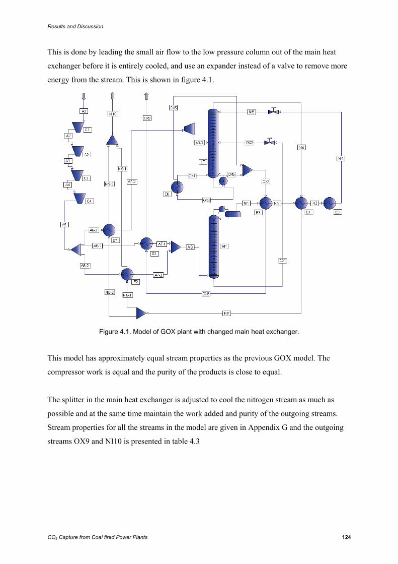
Results and Discussion
CO2 Capture from Coal fired Power Plants 124
This is done by leading the small air flow to the low pressure column out of the main heat
exchanger before it is entirely cooled, and use an expander instead of a valve to remove more
energy from the stream. This is shown in figure 4.1.
Figure 4.1. Model of GOX plant with changed main heat exchanger.
This model has approximately equal stream properties as the previous GOX model. The
compressor work is equal and the purity of the products is close to equal.
The splitter in the main heat exchanger is adjusted to cool the nitrogen stream as much as
possible and at the same time maintain the work added and purity of the outgoing streams.
Stream properties for all the streams in the model are given in Appendix G and the outgoing
streams OX9 and NI10 is presented in table 4.3
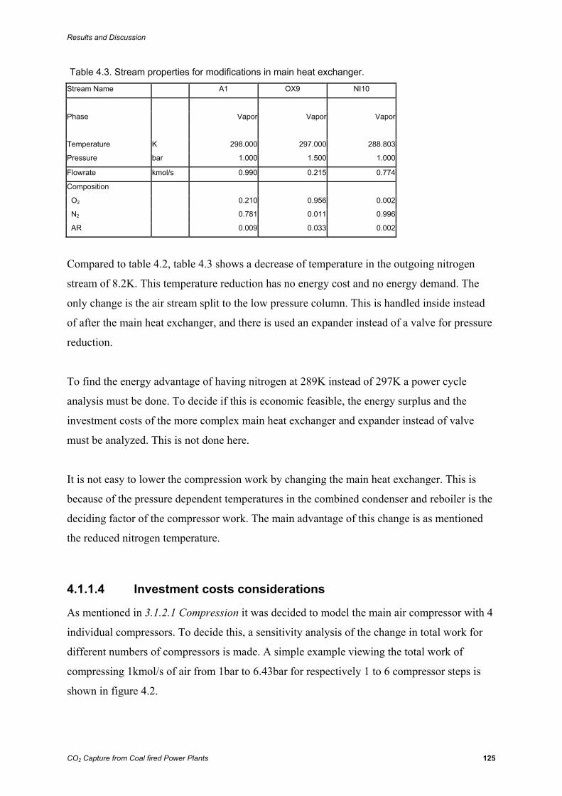
Results and Discussion
CO2 Capture from Coal fired Power Plants 125
Table 4.3. Stream properties for modifications in main heat exchanger.
Stream Name A1 OX9 NI10
Phase Vapor Vapor Vapor
Temperature K 298.000 297.000 288.803
Pressure bar 1.000 1.500 1.000
Flowrate kmol/s 0.990 0.215 0.774
Composition
O2 0.210 0.956 0.002
N2 0.781 0.011 0.996
AR 0.009 0.033 0.002
Compared to table 4.2, table 4.3 shows a decrease of temperature in the outgoing nitrogen
stream of 8.2K. This temperature reduction has no energy cost and no energy demand. The
only change is the air stream split to the low pressure column. This is handled inside instead
of after the main heat exchanger, and there is used an expander instead of a valve for pressure
reduction.
To find the energy advantage of having nitrogen at 289K instead of 297K a power cycle
analysis must be done. To decide if this is economic feasible, the energy surplus and the
investment costs of the more complex main heat exchanger and expander instead of valve
must be analyzed. This is not done here.
It is not easy to lower the compression work by changing the main heat exchanger. This is
because of the pressure dependent temperatures in the combined condenser and reboiler is the
deciding factor of the compressor work. The main advantage of this change is as mentioned
the reduced nitrogen temperature.
4.1.1.4 Investment costs considerations
As mentioned in 3.1.2.1 Compression it was decided to model the main air compressor with 4
individual compressors. To decide this, a sensitivity analysis of the change in total work for
different numbers of compressors is made. A simple example viewing the total work of
compressing 1kmol/s of air from 1bar to 6.43bar for respectively 1 to 6 compressor steps is
shown in figure 4.2.
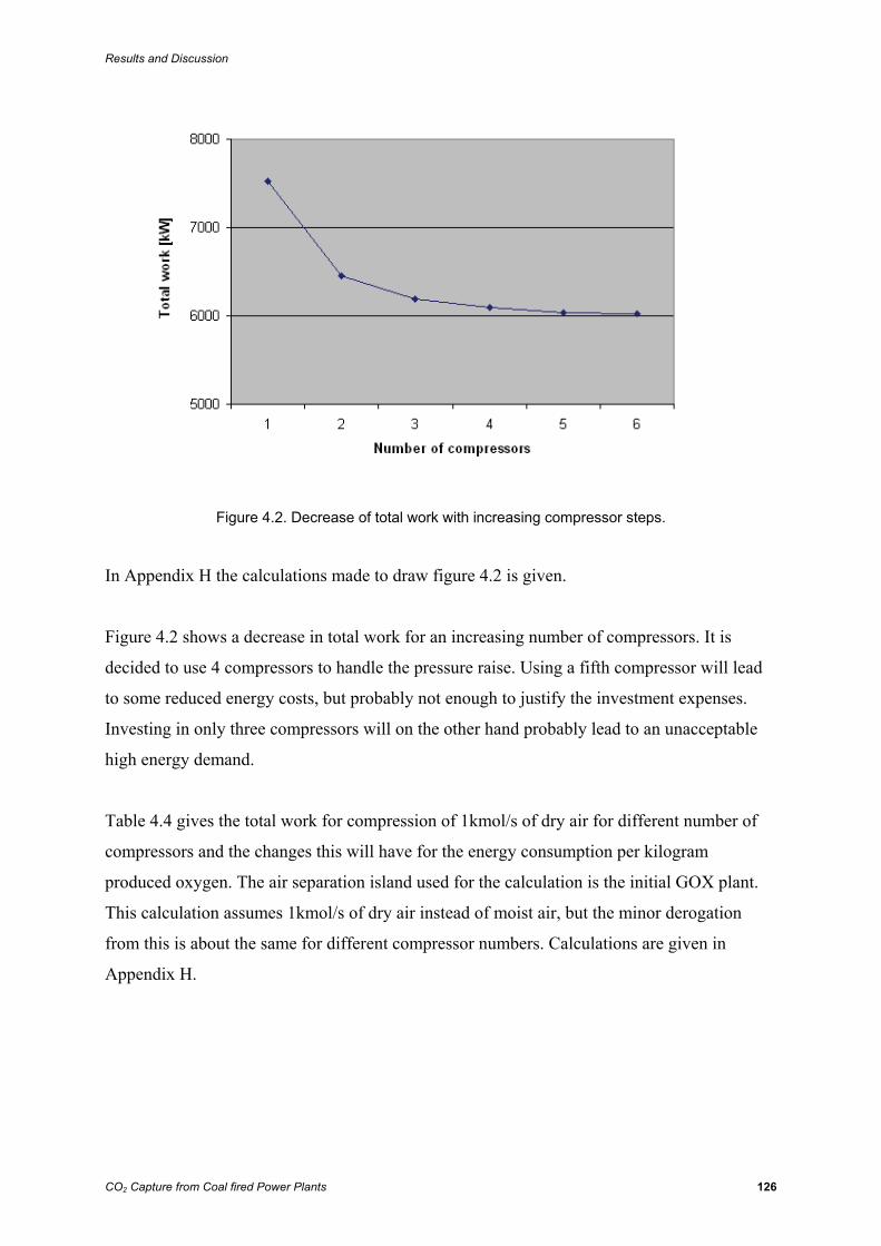
Results and Discussion
CO2 Capture from Coal fired Power Plants 126
Figure 4.2. Decrease of total work with increasing compressor steps.
In Appendix H the calculations made to draw figure 4.2 is given.
Figure 4.2 shows a decrease in total work for an increasing number of compressors. It is
decided to use 4 compressors to handle the pressure raise. Using a fifth compressor will lead
to some reduced energy costs, but probably not enough to justify the investment expenses.
Investing in only three compressors will on the other hand probably lead to an unacceptable
high energy demand.
Table 4.4 gives the total work for compression of 1kmol/s of dry air for different number of
compressors and the changes this will have for the energy consumption per kilogram
produced oxygen. The air separation island used for the calculation is the initial GOX plant.
This calculation assumes 1kmol/s of dry air instead of moist air, but the minor derogation
from this is about the same for different compressor numbers. Calculations are given in
Appendix H.
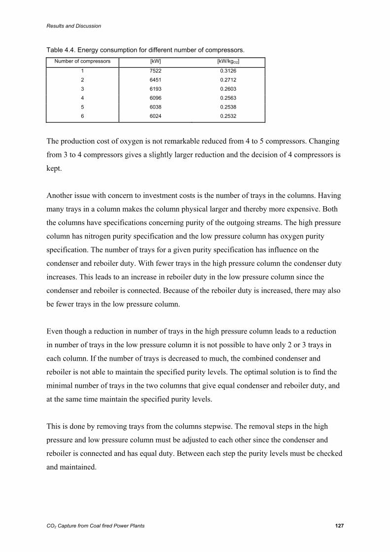
Results and Discussion
CO2 Capture from Coal fired Power Plants 127
Table 4.4. Energy consumption for different number of compressors. Number of compressors [kW] [kW/kgO2]
1 7522 0.3126
2 6451 0.2712
3 6193 0.2603
4 6096 0.2563
5 6038 0.2538
6 6024 0.2532
The production cost of oxygen is not remarkable reduced from 4 to 5 compressors. Changing
from 3 to 4 compressors gives a slightly larger reduction and the decision of 4 compressors is
kept.
Another issue with concern to investment costs is the number of trays in the columns. Having
many trays in a column makes the column physical larger and thereby more expensive. Both
the columns have specifications concerning purity of the outgoing streams. The high pressure
column has nitrogen purity specification and the low pressure column has oxygen purity
specification. The number of trays for a given purity specification has influence on the
condenser and reboiler duty. With fewer trays in the high pressure column the condenser duty
increases. This leads to an increase in reboiler duty in the low pressure column since the
condenser and reboiler is connected. Because of the reboiler duty is increased, there may also
be fewer trays in the low pressure column.
Even though a reduction in number of trays in the high pressure column leads to a reduction
in number of trays in the low pressure column it is not possible to have only 2 or 3 trays in
each column. If the number of trays is decreased to much, the combined condenser and
reboiler is not able to maintain the specified purity levels. The optimal solution is to find the
minimal number of trays in the two columns that give equal condenser and reboiler duty, and
at the same time maintain the specified purity levels.
This is done by removing trays from the columns stepwise. The removal steps in the high
pressure and low pressure column must be adjusted to each other since the condenser and
reboiler is connected and has equal duty. Between each step the purity levels must be checked
and maintained.
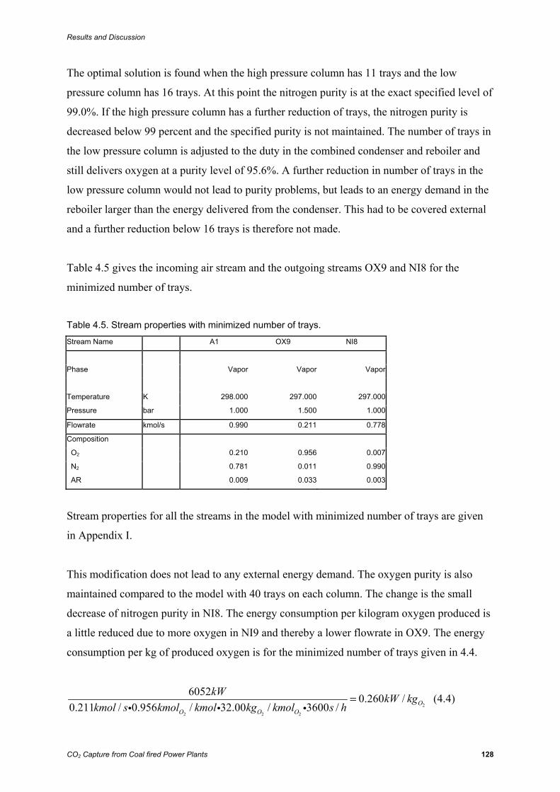
Results and Discussion
CO2 Capture from Coal fired Power Plants 128
The optimal solution is found when the high pressure column has 11 trays and the low
pressure column has 16 trays. At this point the nitrogen purity is at the exact specified level of
99.0%. If the high pressure column has a further reduction of trays, the nitrogen purity is
decreased below 99 percent and the specified purity is not maintained. The number of trays in
the low pressure column is adjusted to the duty in the combined condenser and reboiler and
still delivers oxygen at a purity level of 95.6%. A further reduction in number of trays in the
low pressure column would not lead to purity problems, but leads to an energy demand in the
reboiler larger than the energy delivered from the condenser. This had to be covered external
and a further reduction below 16 trays is therefore not made.
Table 4.5 gives the incoming air stream and the outgoing streams OX9 and NI8 for the
minimized number of trays.
Table 4.5. Stream properties with minimized number of trays.
Stream Name A1 OX9 NI8
Phase Vapor Vapor Vapor
Temperature K 298.000 297.000 297.000
Pressure bar 1.000 1.500 1.000
Flowrate kmol/s 0.990 0.211 0.778
Composition
O2 0.210 0.956 0.007
N2 0.781 0.011 0.990
AR 0.009 0.033 0.003
Stream properties for all the streams in the model with minimized number of trays are given
in Appendix I.
This modification does not lead to any external energy demand. The oxygen purity is also
maintained compared to the model with 40 trays on each column. The change is the small
decrease of nitrogen purity in NI8. The energy consumption per kilogram oxygen produced is
a little reduced due to more oxygen in NI9 and thereby a lower flowrate in OX9. The energy
consumption per kg of produced oxygen is for the minimized number of trays given in 4.4.
2
2 2 2
6052 0.260 /0.211 / 0.956 / 32.00 / 3600 / O
O O O
kW kW kgkmol s kmol kmol kg kmol s h
=i i i
(4.4)
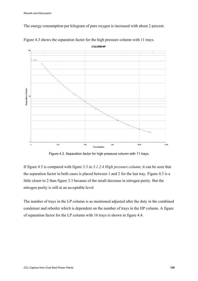
Results and Discussion
CO2 Capture from Coal fired Power Plants 129
The energy consumption per kilogram of pure oxygen is increased with about 2 percent.
Figure 4.3 shows the separation factor for the high pressure column with 11 trays.
Figure 4.3. Separation factor for high pressure column with 11 trays.
If figure 4.3 is compared with figure 3.3 in 3.1.2.4 High pressure column, it can be seen that
the separation factor in both cases is placed between 1 and 2 for the last tray. Figure 4.3 is a
little closer to 2 than figure 3.3 because of the small decrease in nitrogen purity. But the
nitrogen purity is still at an acceptable level.
The number of trays in the LP column is as mentioned adjusted after the duty in the combined
condenser and reboiler which is dependent on the number of trays in the HP column. A figure
of separation factor for the LP column with 16 trays is shown in figure 4.4.
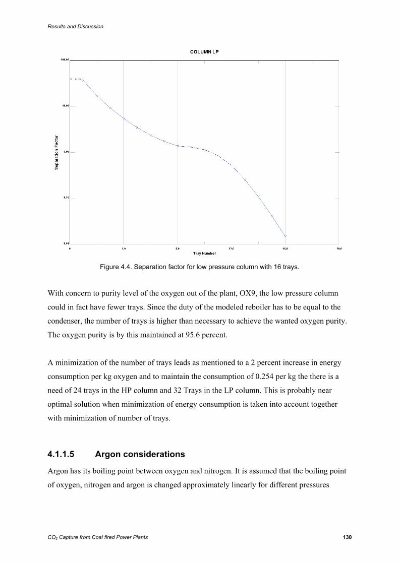
Results and Discussion
CO2 Capture from Coal fired Power Plants 130
Figure 4.4. Separation factor for low pressure column with 16 trays.
With concern to purity level of the oxygen out of the plant, OX9, the low pressure column
could in fact have fewer trays. Since the duty of the modeled reboiler has to be equal to the
condenser, the number of trays is higher than necessary to achieve the wanted oxygen purity.
The oxygen purity is by this maintained at 95.6 percent.
A minimization of the number of trays leads as mentioned to a 2 percent increase in energy
consumption per kg oxygen and to maintain the consumption of 0.254 per kg the there is a
need of 24 trays in the HP column and 32 Trays in the LP column. This is probably near
optimal solution when minimization of energy consumption is taken into account together
with minimization of number of trays.
4.1.1.5 Argon considerations
Argon has its boiling point between oxygen and nitrogen. It is assumed that the boiling point
of oxygen, nitrogen and argon is changed approximately linearly for different pressures
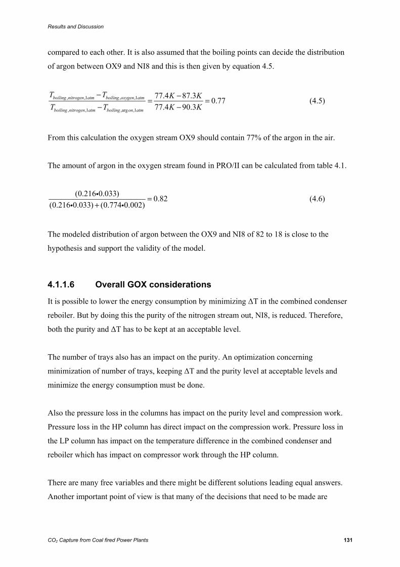
Results and Discussion
CO2 Capture from Coal fired Power Plants 131
compared to each other. It is also assumed that the boiling points can decide the distribution
of argon between OX9 and NI8 and this is then given by equation 4.5.
, ,1 , ,1
, ,1 ,arg ,1
77.4 87.3 0.7777.4 90.3
boiling nitrogen atm boiling oxygen atm
boiling nitrogen atm boiling on atm
T T K KT T K K
− −= =− −
(4.5)
From this calculation the oxygen stream OX9 should contain 77% of the argon in the air.
The amount of argon in the oxygen stream found in PRO/II can be calculated from table 4.1.
(0.216 0.033) 0.82(0.216 0.033) (0.774 0.002)
=+i
i i (4.6)
The modeled distribution of argon between the OX9 and NI8 of 82 to 18 is close to the
hypothesis and support the validity of the model.
4.1.1.6 Overall GOX considerations
It is possible to lower the energy consumption by minimizing ΔT in the combined condenser
reboiler. But by doing this the purity of the nitrogen stream out, NI8, is reduced. Therefore,
both the purity and ΔT has to be kept at an acceptable level.
The number of trays also has an impact on the purity. An optimization concerning
minimization of number of trays, keeping ΔT and the purity level at acceptable levels and
minimize the energy consumption must be done.
Also the pressure loss in the columns has impact on the purity level and compression work.
Pressure loss in the HP column has direct impact on the compression work. Pressure loss in
the LP column has impact on the temperature difference in the combined condenser and
reboiler which has impact on compressor work through the HP column.
There are many free variables and there might be different solutions leading equal answers.
Another important point of view is that many of the decisions that need to be made are
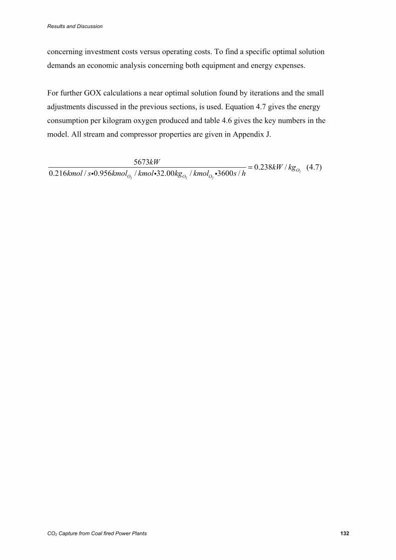
Results and Discussion
CO2 Capture from Coal fired Power Plants 132
concerning investment costs versus operating costs. To find a specific optimal solution
demands an economic analysis concerning both equipment and energy expenses.
For further GOX calculations a near optimal solution found by iterations and the small
adjustments discussed in the previous sections, is used. Equation 4.7 gives the energy
consumption per kilogram oxygen produced and table 4.6 gives the key numbers in the
model. All stream and compressor properties are given in Appendix J.
2
2 2 2
5673 0.238 /0.216 / 0.956 / 32.00 / 3600 / O
O O O
kW kW kgkmol s kmol kmol kg kmol s h
=i i i
(4.7)
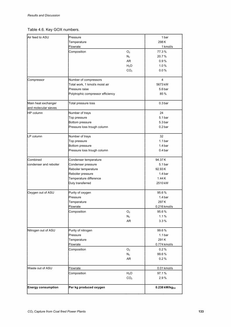
Results and Discussion
CO2 Capture from Coal fired Power Plants 133
Table 4.6. Key GOX numbers.
Air feed to ASU Pressure 1 bar Temperature 298 K Flowrate 1 kmol/s Composition O2 77.3 % N2 20.7 % AR 0.9 % H2O 1.0 % CO2 0.0 % Compressor Number of compressors 4 Total work, 1 kmol/s moist air 5673 kW Pressure raise 5.6 bar Polytrophic compressor efficiency 85 % Main heat exchanger Total pressure loss 0.3 bar and molecular sieves HP column Number of trays 24 Top pressure 5.1 bar Bottom pressure 5.3 bar Pressure loss trough column 0.2 bar LP column Number of trays 32 Top pressure 1.1 bar Bottom pressure 1.4 bar Pressure loss trough column 0.4 bar Combined Condenser temperature 94.37 K condenser and reboiler Condenser pressure 5.1 bar Reboiler temperature 92.93 K Reboiler pressure 1.4 bar Temperature difference 1.44 K Duty transferred 2510 kW Oxygen out of ASU Purity of oxygen 95.6 % Pressure 1.4 bar Temperature 297 K Flowrate 0.216 kmol/s Composition O2 95.6 % N2 1.1 % AR 3.3 % Nitrogen out of ASU Purity of nitrogen 99.6 % Pressure 1.1 bar Temperature 291 K Flowrate 0.774 kmol/s Composition O2 0.2 % N2 99.6 % AR 0.2 % Waste out of ASU Flowrate 0.01 kmol/s Composition H2O 97.1 % CO2 2.9 % Energy consumption Per kg produced oxygen 0.238 kW/kgO2
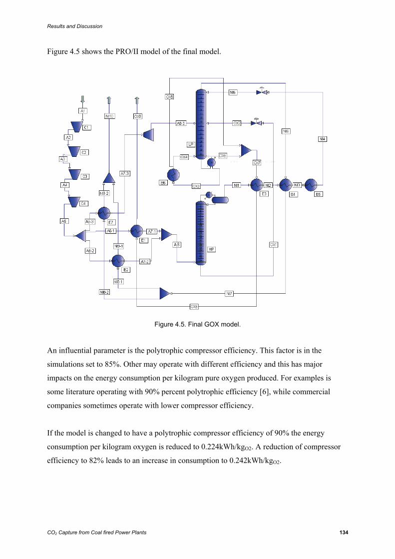
Results and Discussion
CO2 Capture from Coal fired Power Plants 134
Figure 4.5 shows the PRO/II model of the final model.
Figure 4.5. Final GOX model.
An influential parameter is the polytrophic compressor efficiency. This factor is in the
simulations set to 85%. Other may operate with different efficiency and this has major
impacts on the energy consumption per kilogram pure oxygen produced. For examples is
some literature operating with 90% percent polytrophic efficiency [6], while commercial
companies sometimes operate with lower compressor efficiency.
If the model is changed to have a polytrophic compressor efficiency of 90% the energy
consumption per kilogram oxygen is reduced to 0.224kWh/kgO2. A reduction of compressor
efficiency to 82% leads to an increase in consumption to 0.242kWh/kgO2.
Results and Discussion
CO2 Capture from Coal fired Power Plants 135
4.1.2 Liquid oxygen
The LOX model is as mentioned in 3.1.3 Liquid oxygen, an expansion of the GOX model.
The energy consumption per kilogram oxygen produced is not as straight forward presented
as for a GOX plant. The GOX model has an energy consumption given for oxygen at about
ambient conditions. The point of a LOX plant is to deliver oxygen out of ASU at high
pressure and to compare direct with a GOX model is unfair. To be able to compare, the
oxygen flow from the GOX model needs to be compressed to an equal pressure to the LOX
model.
The chosen pressure level is adjusted to the pressure wanted in the gasifier. This pressure is
set to 42bar. To compare the models, the pump in the LOX model and the oxygen compressor
in the end of the GOX model, are both set to have an outcome pressure of 42bar.
The LOX plant has initially the same specifications as the initial GOX plant. 40 trays in both
HP and LP column and the same pressure levels and losses. The LOX model developed is
very sensitive and small adjustments or regulations may give convergence problems. The
developed LOX model is therefore compared with the GOX plant with equal specifications
and if the results from the LOX look good, the model is optimized.
With equal specifications, the outcome of the two models is also quite similar. The purity and
amount of oxygen and nitrogen is in fact exact equal. Stream specifications for all streams in
the LOX model are given in Appendix K and a figure of the model is shown in 3.1.3 Liquid
oxygen.
Because of equal amounts and purities in the two models, compression work is the only factor
needed to be compared. The GOX model has compression work in the main heat exchanger
and in the oxygen compressor. To model an as comparable model as possible, the oxygen
compressor is modeled in two steps. This is done to have comparable lifting heights in the
booster air compressor in the LOX model and the oxygen compressor in the GOX model.

Results and Discussion
CO2 Capture from Coal fired Power Plants 136
The LOX model has compression work in the main heat exchanger, the mentioned booster air
compressor and a small pump work in the oxygen pump. The compressor information for the
two models is presented in table 4.7 and 4.8.
Table 4.7. Compression work initial GOX model.
Compressor Name C1 C2 C3 C4 C5 C6
Main Main Main Main Air Air
Pressure bar 1.600 2.500 4.000 6.430 6.300 42.000
Temperature K 348.940 348.389 351.332 351.905 476.891 554.210
Head m 5224.165 5166.875 5468.312 5525.645 16895.041 24386.836
Actual Work kW 1469.220 1453.108 1537.882 1554.007 1153.192 1663.127
Isentropic coef., k 1.401 1.402 1.404 1.407 1.396 1.406
Table 4.8. Compression work initial LOX model.
Compressor Name C1 C2 C3 C4 C5 P1
Main Main Main Main Booster Pump
Pressure bar 1.600 2.500 4.000 6.430 40.000 42.000
Temperature K 348.940 348.193 351.332 351.905 550.815 n/a
Head m 5224.165 5163.930 5468.312 5525.645 26404.031 200.084
Actual Work kW 1469.220 1745.669 1848.566 1867.947 2250.226 15.146
Isentropic coef., k 1.401 1.402 1.404 1.407 1.417 n/a
This gives a total work demand of 8831 kW for the GOX model and 9197 kW for the LOX
model. This equals a 4 percent higher energy demand in the LOX model than the GOX
model.
The LOX production method described in 2.1.2.10 Liquid oxygen in the theoretical
background feeds the booster compressed air to the high pressure column. This is not possible
in the model developed in this report. The model developed here has a need of cooling in the
subcooler, in the nitrogen stream between the HP and LP column. As mentioned in 3.1.3.2
Minimum temperature approach problems, the booster compressed air is not cold enough to
cool the nitrogen stream when choked to HP pressure level. Therefore it has to be choked
lower than HP pressure and a need of recompression occurs. This leads to increased work in
the main compressor making the LOX model more energy demanding than the GOX model.

Results and Discussion
CO2 Capture from Coal fired Power Plants 137
Due to higher energy demand in the LOX model compared to the initial GOX model, further
optimization of the LOX model is not prioritized. The solution of 0.238 kWh per kilogram of
produced oxygen presented in 4.1.1.6 Overall GOX considerations is used in further
calculations.
Results and Discussion
CO2 Capture from Coal fired Power Plants 138
4.2 Gasification Island
4.2.1 Introduction
Calculations and modeling on gasification of three different coals are described in the method
part. Here the results will be presented and discussed. Results from MatLab calculations,
PRO/II and GTPRO simulations and other calculations are presented in the upcoming
chapters.
4.2.2 MatLab calculations
The MatLab program calculates the equilibrium conditions based on elements and not as
molecules. This will give other molar fractions since H2, O2 and N2 have other molecular
weights than H, O and N. The compositions of the three coals as elements are presented in
table 4.9. The amount of O2 and H2O for the gasification process is the same as the amounts
found from the PRO/II simulations. These numbers are discussed closer in 4.2.3 Pro/II
simulations.
Table 4.9. Molar fractions for MatLab calculations.
Coal Mol Fraction Reactants
Region Classification C H O N S H2O O2 H2O
Rhein Browncoal 0.569 0.126 0.041 0.001 0.002 0.261 0.179 0.000
Datung Bituminous 0.597 0.346 0.050 0.005 0.002 0.000 0.280 0.130
Ruhr Anthracite 0.679 0.296 0.014 0.009 0.002 0.000 0.300 0.200
It should be noted that for the Browncoal the H2O is included in the total composition. This
indicates that it is a model of a wet slurry coal feed.
The feed from table 4.9 calculated with the MatLab equilibrium calculator give the following
molar fractions of syngas. These calculations only show the CO, CO2, H2 and H2O because of
the mentioned convergence problems using all the elements. It is however the most relevant
gasses that is presented here.
Results and Discussion
CO2 Capture from Coal fired Power Plants 139
Table 4.10. Syngas composition for different coals calculated in MatLab.
Coal Browncoal Browncoal Bituminous Bituminous Anthracite Anthracite
Temperature C 1481 1481 1572 1572 1233 1233
Pressure Bar 42 42 42 42 42 42
syngas composition Mole fraction
Dry mole fraction Mole fraction
Dry mole fraction Mole fraction
Dry mole fraction
CO 0.601 0.643 0.601 0.666 0.600 0.645
CO2 0.037 0.040 0.062 0.069 0.061 0.066
H2 0.298 0.319 0.239 0.265 0.269 0.289
H2O 0.065 0.000 0.098 0.000 0.070 0.000
The temperatures here are equivalent with the ones from the PRO/II simulations discussed in
the next chapter. The literature handles with gas analysis on dry basis. Therefore the water is
removed to get comparable results. The shaded columns show the molar fractions on dry
basis. To calculate the dry gas composition the water content in the syngas is removed. An
example of this calculation is shown for CO and H2 for the Browncoal in table 4.10.
2
0.601 0.6431 1 0.065dry
coco
H O
yyy
= = =− −
(4.8)
2
2
2
0.298 0.3191 1 0.065dry
HH
H O
yy
y= = =
− − (4.9)
4.2.3 PRO/II simulations
The results from the PRO/II simulations on three different coals will be presented here.
Finding the oxygen (and steam) amount and to get a syngas composition close to the one
found in literature is the main goal for these calculations.
4.2.3.1 Gasification of Browncoal
Table 4.11 gives the different flow rates from the PRO/II calculation of the Browncoal. The
coal contains considerable amount of water and the only gasification agent is therefore the
oxygen. The column to the right is showing the syngas at normal state. This is calculated
using the method presented in 3.2.4.2 Modeling Gasification Island, and is only interesting

Results and Discussion
CO2 Capture from Coal fired Power Plants 140
for comparing with given literature. A heat exchanger that normalizes the product gas will not
be included in a gasification plant and is only used as a calculation tool.
Table 4.11. Different flow rates for Browncoal gasification. Coal Oxygen Syngas Nm3 Syngas
Temperature C 25.000 25.000 1480.743 15.000
Pressure Bar 42.000 42.000 41.600 1.013
Rate kmol/s 1.000 0.179 0.931 0.931
kg/s 12.692 5.728 18.420 18.420
Actual Rate m3/s 0.173 0.104 3.276 17.359
Standard Vapor Rate m3/s 6.460 4.012 20.862 16.452
The amounts of oxygen (and steam) were found doing iteration between syngas composition,
temperature and amount of the different feed. The results from this will be presented here.
Nm3 syngas / ton maf coal The rate of produced syngas can be calculated from table 4.11 and table 4.12. Syngas is
defined as CO and H2 and therefore will only these substances be included in the calculation.
From Table 4.12 the syngas fraction can be found, 0.502CO + 0.246H2 = 0.748syngas. The
normalized flow is found from table 4.11 to be 17.359 and the volume flow of syngas at
normal conditions then becomes 17.359·0.748 = 12.985 Nm3. The mass flow is taken directly
from Table 4.11, 12.692 kg/s. These numbers are then adjusted to get the rate at Nm3/ton
form.
[ ]3 312.985
1000 102312.692
Nm kg Nmkg ton ton
⎡ ⎤ ⎡ ⎤⎡ ⎤⎣ ⎦ = ⎢ ⎥⎢ ⎥⎣ ⎦ ⎣ ⎦i (4.10)
Nm3 O2 / Nm3 Syngas The consumption of oxygen per m3 syngas can be calculated directly from the table using the
standard vapor rate since the correlation between standard and normal condition is the same
for O2 and syngas. 3
3
4.0120.326
0.748 16.452
Sm
Sm
⎡ ⎤⎣ ⎦ =⎡ ⎤⎣ ⎦i
(4.11)
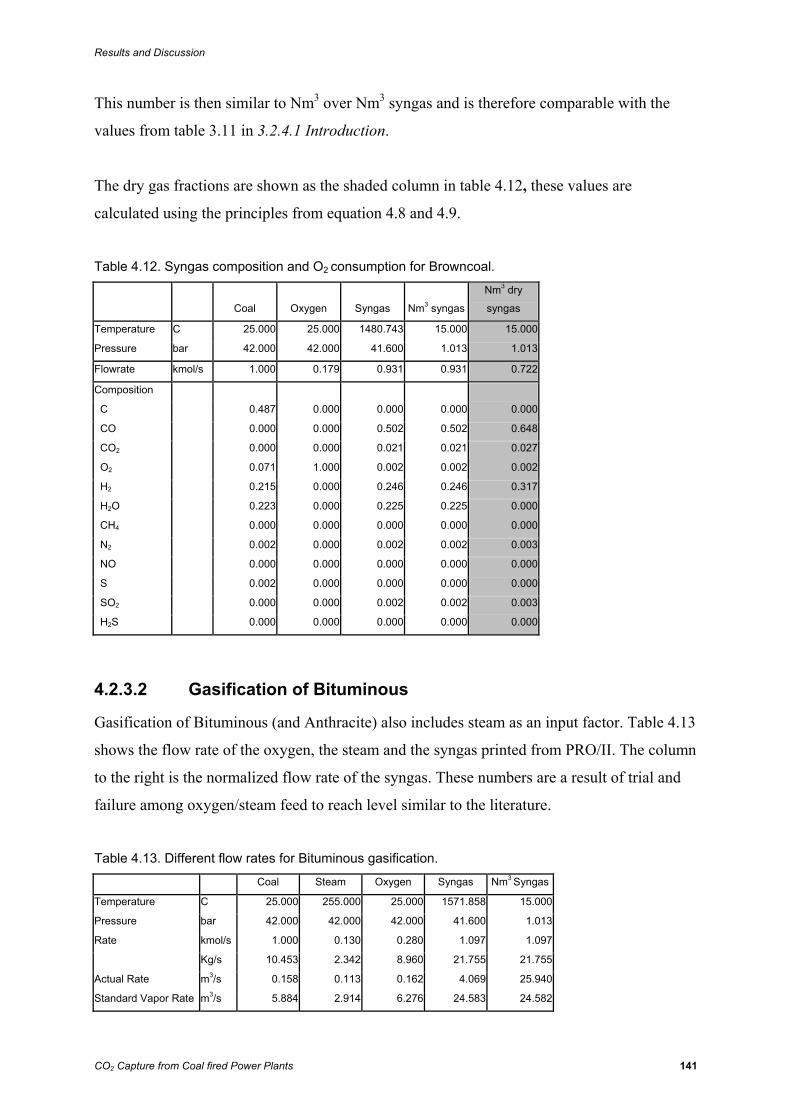
Results and Discussion
CO2 Capture from Coal fired Power Plants 141
This number is then similar to Nm3 over Nm3 syngas and is therefore comparable with the
values from table 3.11 in 3.2.4.1 Introduction.
The dry gas fractions are shown as the shaded column in table 4.12, these values are
calculated using the principles from equation 4.8 and 4.9.
Table 4.12. Syngas composition and O2 consumption for Browncoal.
Coal Oxygen Syngas Nm3 syngas
Nm3 dry
syngas
Temperature C 25.000 25.000 1480.743 15.000 15.000
Pressure bar 42.000 42.000 41.600 1.013 1.013
Flowrate kmol/s 1.000 0.179 0.931 0.931 0.722
Composition
C 0.487 0.000 0.000 0.000 0.000
CO 0.000 0.000 0.502 0.502 0.648
CO2 0.000 0.000 0.021 0.021 0.027
O2 0.071 1.000 0.002 0.002 0.002
H2 0.215 0.000 0.246 0.246 0.317
H2O 0.223 0.000 0.225 0.225 0.000
CH4 0.000 0.000 0.000 0.000 0.000
N2 0.002 0.000 0.002 0.002 0.003
NO 0.000 0.000 0.000 0.000 0.000
S 0.002 0.000 0.000 0.000 0.000
SO2 0.000 0.000 0.002 0.002 0.003
H2S 0.000 0.000 0.000 0.000 0.000
4.2.3.2 Gasification of Bituminous
Gasification of Bituminous (and Anthracite) also includes steam as an input factor. Table 4.13
shows the flow rate of the oxygen, the steam and the syngas printed from PRO/II. The column
to the right is the normalized flow rate of the syngas. These numbers are a result of trial and
failure among oxygen/steam feed to reach level similar to the literature.
Table 4.13. Different flow rates for Bituminous gasification. Coal Steam Oxygen Syngas Nm3 Syngas
Temperature C 25.000 255.000 25.000 1571.858 15.000
Pressure bar 42.000 42.000 42.000 41.600 1.013
Rate kmol/s 1.000 0.130 0.280 1.097 1.097
Kg/s 10.453 2.342 8.960 21.755 21.755
Actual Rate m3/s 0.158 0.113 0.162 4.069 25.940
Standard Vapor Rate m3/s 5.884 2.914 6.276 24.583 24.582
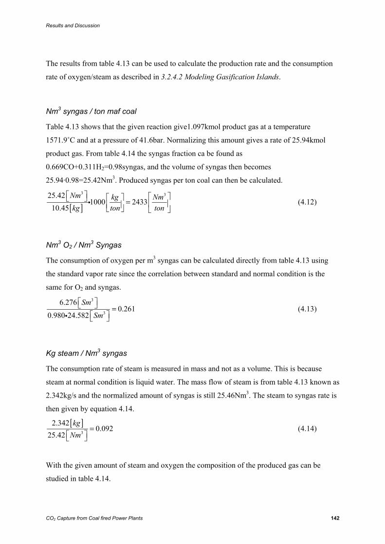
Results and Discussion
CO2 Capture from Coal fired Power Plants 142
The results from table 4.13 can be used to calculate the production rate and the consumption
rate of oxygen/steam as described in 3.2.4.2 Modeling Gasification Islands.
Nm3 syngas / ton maf coal
Table 4.13 shows that the given reaction give1.097kmol product gas at a temperature
1571.9˚C and at a pressure of 41.6bar. Normalizing this amount gives a rate of 25.94kmol
product gas. From table 4.14 the syngas fraction ca be found as
0.669CO+0.311H2=0.98syngas, and the volume of syngas then becomes
25.94·0.98=25.42Nm3. Produced syngas per ton coal can then be calculated.
[ ]3 325.42
1000 243310.45
Nm kg Nmkg ton ton
⎡ ⎤ ⎡ ⎤⎡ ⎤⎣ ⎦ = ⎢ ⎥⎢ ⎥⎣ ⎦ ⎣ ⎦i (4.12)
Nm3 O2 / Nm3 Syngas
The consumption of oxygen per m3 syngas can be calculated directly from table 4.13 using
the standard vapor rate since the correlation between standard and normal condition is the
same for O2 and syngas. 3
3
6.2760.261
0.980 24.582
Sm
Sm
⎡ ⎤⎣ ⎦ =⎡ ⎤⎣ ⎦i
(4.13)
Kg steam / Nm3 syngas
The consumption rate of steam is measured in mass and not as a volume. This is because
steam at normal condition is liquid water. The mass flow of steam is from table 4.13 known as
2.342kg/s and the normalized amount of syngas is still 25.46Nm3. The steam to syngas rate is
then given by equation 4.14.
[ ]3
2.3420.092
25.42kg
Nm=
⎡ ⎤⎣ ⎦ (4.14)
With the given amount of steam and oxygen the composition of the produced gas can be
studied in table 4.14.
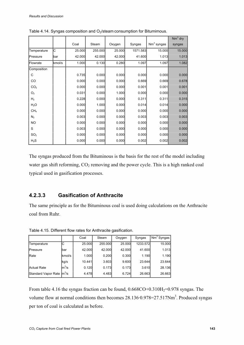
Results and Discussion
CO2 Capture from Coal fired Power Plants 143
Table 4.14. Syngas composition and O2/steam consumption for Bitumimous.
Coal Steam Oxygen Syngas Nm3 syngas
Nm3 dry
syngas
Temperature C 25.000 255.000 25.000 1571.583 15.000 15.000
Pressure bar 42.000 42.000 42.000 41.600 1.013 1.013
Flowrate kmol/s 1.000 0.130 0.280 1.097 1.097 1.082
Composition
C 0.735 0.000 0.000 0.000 0.000 0.000
CO 0.000 0.000 0.000 0.669 0.669 0.678
CO2 0.000 0.000 0.000 0.001 0.001 0.001
O2 0.031 0.000 1.000 0.000 0.000 0.000
H2 0.228 0.000 0.000 0.311 0.311 0.315
H2O 0.000 1.000 0.000 0.014 0.014 0.000
CH4 0.000 0.000 0.000 0.000 0.000 0.000
N2 0.003 0.000 0.000 0.003 0.003 0.003
NO 0.000 0.000 0.000 0.000 0.000 0.000
S 0.003 0.000 0.000 0.000 0.000 0.000
SO2 0.000 0.000 0.000 0.000 0.000 0.000
H2S 0.000 0.000 0.000 0.002 0.002 0.002
The syngas produced from the Bituminous is the basis for the rest of the model including
water gas shift reforming, CO2 removing and the power cycle. This is a high ranked coal
typical used in gasification processes.
4.2.3.3 Gasification of Anthracite
The same principle as for the Bituminous coal is used doing calculations on the Anthracite
coal from Ruhr.
Table 4.15. Different flow rates for Anthracite gasification. Coal Steam Oxygen Syngas Nm3 Syngas
Temperature C 25.000 255.000 25.000 1233.572 15.000
Pressure bar 42.000 42.000 42.000 41.600 1.013
Rate kmol/s 1.000 0.200 0.300 1.190 1.190
kg/s 10.441 3.603 9.600 23.644 23.644
Actual Rate m3/s 0.120 0.173 0.173 3.610 28.136
Standard Vapor Rate m3/s 4.478 4.483 6.724 26.663 26.663
From table 4.16 the syngas fraction can be found, 0.668CO+0.310H2=0.978 syngas. The
volume flow at normal conditions then becomes 28.136·0.978=27.517Nm3. Produced syngas
per ton of coal is calculated as before.
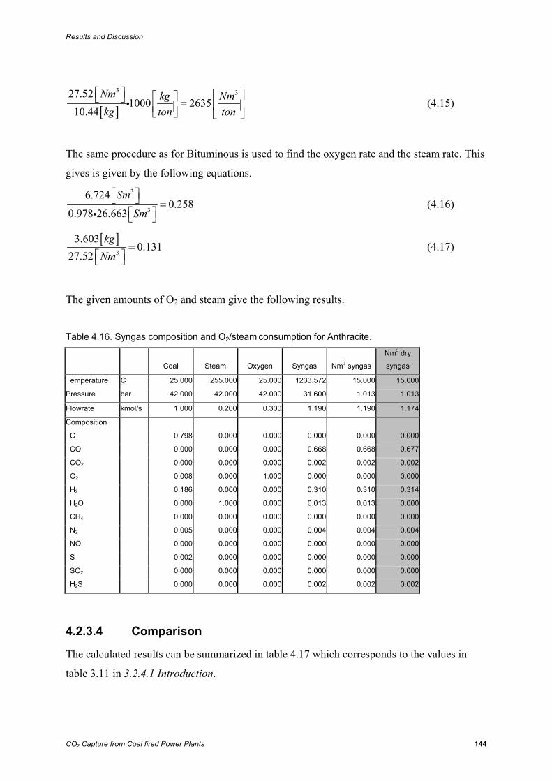
Results and Discussion
CO2 Capture from Coal fired Power Plants 144
[ ]3 327.52
1000 263510.44
Nm kg Nmkg ton ton
⎡ ⎤ ⎡ ⎤⎡ ⎤⎣ ⎦ = ⎢ ⎥⎢ ⎥⎣ ⎦ ⎣ ⎦i (4.15)
The same procedure as for Bituminous is used to find the oxygen rate and the steam rate. This
gives is given by the following equations. 3
3
6.7240.258
0.978 26.663
Sm
Sm
⎡ ⎤⎣ ⎦ =⎡ ⎤⎣ ⎦i
(4.16)
[ ]3
3.6030.131
27.52kg
Nm=
⎡ ⎤⎣ ⎦ (4.17)
The given amounts of O2 and steam give the following results.
Table 4.16. Syngas composition and O2/steam consumption for Anthracite.
Coal Steam Oxygen Syngas Nm3 syngas
Nm3 dry
syngas
Temperature C 25.000 255.000 25.000 1233.572 15.000 15.000
Pressure bar 42.000 42.000 42.000 31.600 1.013 1.013
Flowrate kmol/s 1.000 0.200 0.300 1.190 1.190 1.174
Composition
C 0.798 0.000 0.000 0.000 0.000 0.000
CO 0.000 0.000 0.000 0.668 0.668 0.677
CO2 0.000 0.000 0.000 0.002 0.002 0.002
O2 0.008 0.000 1.000 0.000 0.000 0.000
H2 0.186 0.000 0.000 0.310 0.310 0.314
H2O 0.000 1.000 0.000 0.013 0.013 0.000
CH4 0.000 0.000 0.000 0.000 0.000 0.000
N2 0.005 0.000 0.000 0.004 0.004 0.004
NO 0.000 0.000 0.000 0.000 0.000 0.000
S 0.002 0.000 0.000 0.000 0.000 0.000
SO2 0.000 0.000 0.000 0.000 0.000 0.000
H2S 0.000 0.000 0.000 0.002 0.002 0.002
4.2.3.4 Comparison
The calculated results can be summarized in table 4.17 which corresponds to the values in
table 3.11 in 3.2.4.1 Introduction.
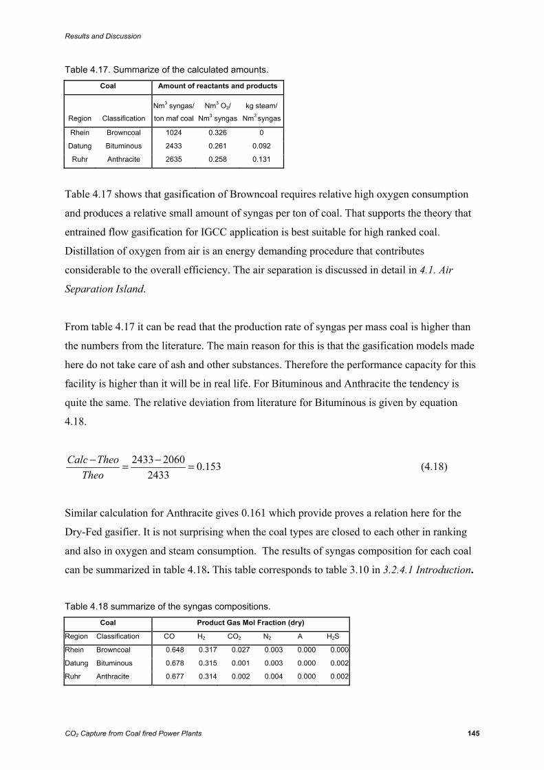
Results and Discussion
CO2 Capture from Coal fired Power Plants 145
Table 4.17. Summarize of the calculated amounts.
Coal Amount of reactants and products
Region Classification
Nm3 syngas/
ton maf coal
Nm3 O2/
Nm3 syngas
kg steam/
Nm3 syngas
Rhein Browncoal 1024 0.326 0
Datung Bituminous 2433 0.261 0.092
Ruhr Anthracite 2635 0.258 0.131
Table 4.17 shows that gasification of Browncoal requires relative high oxygen consumption
and produces a relative small amount of syngas per ton of coal. That supports the theory that
entrained flow gasification for IGCC application is best suitable for high ranked coal.
Distillation of oxygen from air is an energy demanding procedure that contributes
considerable to the overall efficiency. The air separation is discussed in detail in 4.1. Air
Separation Island.
From table 4.17 it can be read that the production rate of syngas per mass coal is higher than
the numbers from the literature. The main reason for this is that the gasification models made
here do not take care of ash and other substances. Therefore the performance capacity for this
facility is higher than it will be in real life. For Bituminous and Anthracite the tendency is
quite the same. The relative deviation from literature for Bituminous is given by equation
4.18.
2433 2060 0.1532433
Calc TheoTheo
− −= = (4.18)
Similar calculation for Anthracite gives 0.161 which provide proves a relation here for the
Dry-Fed gasifier. It is not surprising when the coal types are closed to each other in ranking
and also in oxygen and steam consumption. The results of syngas composition for each coal
can be summarized in table 4.18. This table corresponds to table 3.10 in 3.2.4.1 Introduction.
Table 4.18 summarize of the syngas compositions.
Coal Product Gas Mol Fraction (dry)
Region Classification CO H2 CO2 N2 A H2S
Rhein Browncoal 0.648 0.317 0.027 0.003 0.000 0.000
Datung Bituminous 0.678 0.315 0.001 0.003 0.000 0.002
Ruhr Anthracite 0.677 0.314 0.002 0.004 0.000 0.002
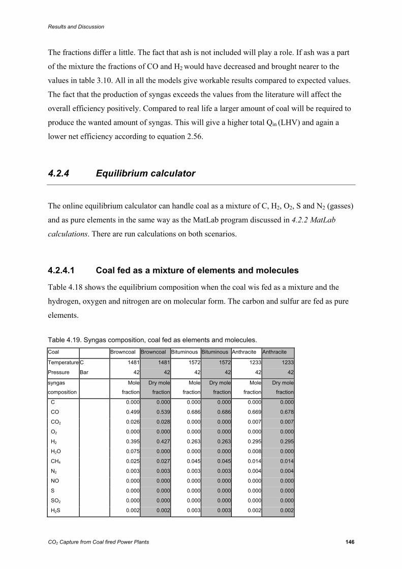
Results and Discussion
CO2 Capture from Coal fired Power Plants 146
The fractions differ a little. The fact that ash is not included will play a role. If ash was a part
of the mixture the fractions of CO and H2 would have decreased and brought nearer to the
values in table 3.10. All in all the models give workable results compared to expected values.
The fact that the production of syngas exceeds the values from the literature will affect the
overall efficiency positively. Compared to real life a larger amount of coal will be required to
produce the wanted amount of syngas. This will give a higher total Qin (LHV) and again a
lower net efficiency according to equation 2.56.
4.2.4 Equilibrium calculator
The online equilibrium calculator can handle coal as a mixture of C, H2, O2, S and N2 (gasses)
and as pure elements in the same way as the MatLab program discussed in 4.2.2 MatLab
calculations. There are run calculations on both scenarios.
4.2.4.1 Coal fed as a mixture of elements and molecules
Table 4.18 shows the equilibrium composition when the coal wis fed as a mixture and the
hydrogen, oxygen and nitrogen are on molecular form. The carbon and sulfur are fed as pure
elements.
Table 4.19. Syngas composition, coal fed as elements and molecules.
Coal Browncoal Browncoal Bituminous Bituminous Anthracite Anthracite
Temperature C 1481 1481 1572 1572 1233 1233
Pressure Bar 42 42 42 42 42 42
syngas
composition
Mole
fraction
Dry mole
fraction
Mole
fraction
Dry mole
fraction
Mole
fraction
Dry mole
fraction
C 0.000 0.000 0.000 0.000 0.000 0.000
CO 0.499 0.539 0.686 0.686 0.669 0.678
CO2 0.026 0.028 0.000 0.000 0.007 0.007
O2 0.000 0.000 0.000 0.000 0.000 0.000
H2 0.395 0.427 0.263 0.263 0.295 0.295
H2O 0.075 0.000 0.000 0.000 0.008 0.000
CH4 0.025 0.027 0.045 0.045 0.014 0.014
N2 0.003 0.003 0.003 0.003 0.004 0.004
NO 0.000 0.000 0.000 0.000 0.000 0.000
S 0.000 0.000 0.000 0.000 0.000 0.000
SO2 0.000 0.000 0.000 0.000 0.000 0.000
H2S 0.002 0.002 0.003 0.003 0.002 0.002
Results and Discussion
CO2 Capture from Coal fired Power Plants 147
The results from table 4.18 show a relation between the PRO/II calculations and the
calculator. The case of Anthracite and Bituminous give much the same values. The main
deviation is that the online calculator gives an amount of CH4 in the products which again
decreases the amount of H2 since 1mole of CH4 contains 1C and 4H. In PRO/II these
substances are distributed among CO, CO2 and H2 and therefore it will give a higher fraction
of H2 due to the molar balance. CH4 is favored by low temperature and this is a likely
explanation of the differences between the two calculations. In PRO/II the temperature is a
function of the fed and will vary during the gasification process, while the calculator does
calculation for given temperatures. For the special case of Browncoal the differences can also
be a result of the feeding of water. For the Dry feed gasifiers the water is fed separately at
255˚C while the Slurry Fed gets the water part included in the coal feed at lower temperature.
In the calculator there is no feeding procedure that differs if the water is a part of the coal or a
separate reactant.
4.2.4.2 Coal fed as elements only
Table 4.20 gives the results from a calculation with pure elements, which means for example
that the hydrogen part of the feed is defined as H instead of H2. That gives different molar
fractions in the feed compared to the case where the feed is presented as both elements and
molecules. An example of a transcript from the online chemical calculator is given in
Appendix L.
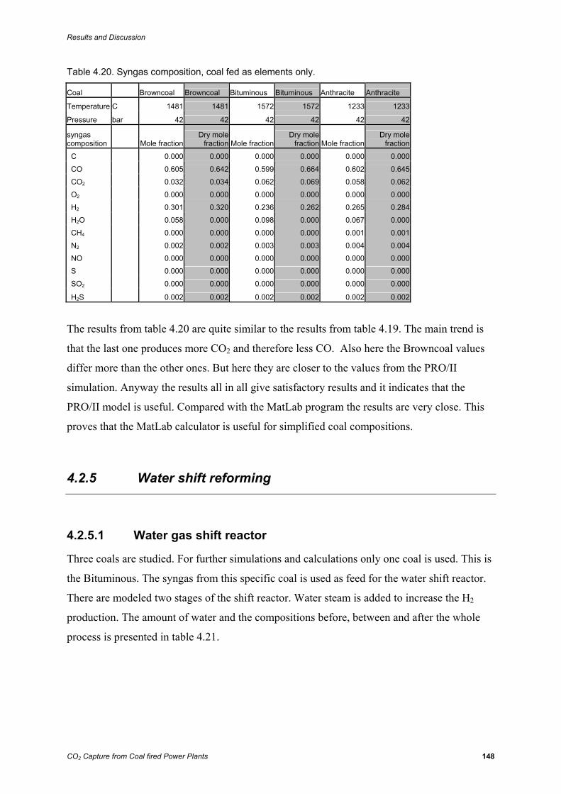
Results and Discussion
CO2 Capture from Coal fired Power Plants 148
Table 4.20. Syngas composition, coal fed as elements only.
Coal Browncoal Browncoal Bituminous Bituminous Anthracite Anthracite
Temperature C 1481 1481 1572 1572 1233 1233
Pressure bar 42 42 42 42 42 42
syngas composition Mole fraction
Dry mole fraction Mole fraction
Dry mole fraction Mole fraction
Dry mole fraction
C 0.000 0.000 0.000 0.000 0.000 0.000
CO 0.605 0.642 0.599 0.664 0.602 0.645
CO2 0.032 0.034 0.062 0.069 0.058 0.062
O2 0.000 0.000 0.000 0.000 0.000 0.000
H2 0.301 0.320 0.236 0.262 0.265 0.284
H2O 0.058 0.000 0.098 0.000 0.067 0.000
CH4 0.000 0.000 0.000 0.000 0.001 0.001
N2 0.002 0.002 0.003 0.003 0.004 0.004
NO 0.000 0.000 0.000 0.000 0.000 0.000
S 0.000 0.000 0.000 0.000 0.000 0.000
SO2 0.000 0.000 0.000 0.000 0.000 0.000
H2S 0.002 0.002 0.002 0.002 0.002 0.002
The results from table 4.20 are quite similar to the results from table 4.19. The main trend is
that the last one produces more CO2 and therefore less CO. Also here the Browncoal values
differ more than the other ones. But here they are closer to the values from the PRO/II
simulation. Anyway the results all in all give satisfactory results and it indicates that the
PRO/II model is useful. Compared with the MatLab program the results are very close. This
proves that the MatLab calculator is useful for simplified coal compositions.
4.2.5 Water shift reforming
4.2.5.1 Water gas shift reactor
Three coals are studied. For further simulations and calculations only one coal is used. This is
the Bituminous. The syngas from this specific coal is used as feed for the water shift reactor.
There are modeled two stages of the shift reactor. Water steam is added to increase the H2
production. The amount of water and the compositions before, between and after the whole
process is presented in table 4.21.

Results and Discussion
CO2 Capture from Coal fired Power Plants 149
Table 4.21. Molar compositions for different stages.
Stream Name
Cooled syngas Steam
Intermediate gas H2-rich gas
Dry-H2 rich gas
Phase Vapor Vapor Vapor Vapor Vapor
Temperature C 250.000 255.000 498.535 294.105 36.670
Pressure bar 41.400 41.400 41.000 40.400 40.200
Flowrate kmol/s 1.097 1.07 2.167 2.167 1.772
Composition C 0.000 0.000 0.000 0.000 0.000
CO 0.669 0.000 0.085 0.020 0.024
CO2 0.001 0.000 0.254 0.319 0.390
O2 0.000 0.000 0.000 0.000 0.000
H2 0.311 0.000 0.411 0.476 0.582
H2O 0.014 1.000 0.247 0.182 0.000
CH4 0.000 0.000 0.000 0.000 0.000
N2 0.003 0.000 0.002 0.002 0.002
NO 0.000 0.000 0.000 0.000 0.000
S 0.000 0.000 0.000 0.000 0.000
SO2 0.000 0.000 0.000 0.000 0.000
H2S 0.002 0.000 0.001 0.001 0.001
The product gas from the first stage has a temperature of 499˚C and this is cooled to 225˚C
before the second stage. This is called the intermediate gas inn the table. The column to the
left shows the composition after the water has been removed. In the first stage there is fed
1.07kmol of steam for this amount of syngas. It should be kept in mind that these numbers are
valid for a coal feed of 1kmol. When it comes to the total plant the amounts will be adjusted
to fit the turbine. The ratio between fed steam and fed CO will be independent of the coal feed
and is for this shift reactor given in equation 4.19.
2 1.097 0.014 1.070 1.000 1.4791.097 0.669
H OCO
+= =i ii
(4.19)
Compared to literature [21] this is a realistic value. The ratio may be as high as 2, however
this will give more H2O in the product gas that has to be condensed before the CO2 capture
unit anyway. There are also limitations according to the fraction of water in the product gas. It
should not exceed 0.2 [10]. In addition is a CO fraction of 0.02 a realistic value. Addition of
more steam is also an energy requiring process so this is seen as a satisfactory result.
Results and Discussion
CO2 Capture from Coal fired Power Plants 150
With these conditions one mole of coal will give 2.167*0.427=1.031kmol of H2. The 2 % of
CO has also heating values and can be fed to a turbine. Normally is H2O an excellent diluter,
but in this case will the combustion process form a relatively high amount of water so the total
amount will be too high for the turbine. The high amount of CO2 makes it relatively easy to
remove it. A molar fraction of 0.390 after the water removing and a total pressure of 40.2bar
gives a partial pressure of CO2 of 15.68bar. This is advantageous for the removing process.
The N2 is low and anyway a good substance to feed together with the H2 rich fuel. More N2
will be fed after the CO2 capture unit before the combustion chamber in the gas turbine.
4.2.5.2 Integrating the gasification and water shift
The temperature of the syngas can be reduced by adding more water into the gasifier. This
again will give more H2O in the syngas and reduce the additional steam demand in the shift
reactor. Allocating the steam/water in other ways gives no considerable changes. The
composition from table 4.21 is therefore sent further to the CO2 capture unit before it is
diluted with nitrogen and fed to the power cycle.
The chosen coal going through the gasifier and two stages of water shift reactors generates
heat in all processes. This is because the overall reactions are more exothermic than
endothermic. This can be expressed in the term of cold gas efficiency. The heating value for
the coal using equation 3.23 is given in equation 4.20.
0.736 393520 0.228 241820 0.003 296800 345656coalkJLHV
kmol⎡ ⎤= + + = ⎢ ⎥⎣ ⎦
i i i (4.20)
The bituminous has a molar weight of 10.455kg/kmol and the LHV becomes on mass basis
345956/10.455=33090kJ/kg. This is much closed to the tabulated value from table 2.3 in
2.2.1.1 composition which operates with a LHV of 33400kJ/kg for Bituminous. LHV for the
CO and H2 mix is then given by equation 4.21.
[ ]1.097 0.669 282990 0.311 241820 290185syngaskJLHV
kmol⎡ ⎤= + = ⎢ ⎥⎣ ⎦
i i i (4.21)
Results and Discussion
CO2 Capture from Coal fired Power Plants 151
This gives a CGE of:
290185 0.840345656
CGE = = (4.22)
This value corresponds to the literature. It is stated that a gasification process requires a CGE
of at least 0.78 to make IGCC attractive [6].
The LHV for the H2 rich fuel is loosing some more heating value and for this case it is given
by equation 4.23.
[ ]2
1.967 0.02 282990 0.527 241820 261806H richkJLHV
kmol⎡ ⎤= + = ⎢ ⎥⎣ ⎦
i i i (4.23)
This indicates that there is a loss in heating values through the process. In an IGCC some of
the heat that is released can be utilized in other processes and improve efficiency. This will be
discussed more in 4.4.2.2 Adding steam to the steam turbine.
Results and Discussion
CO2 Capture from Coal fired Power Plants 152
4.3 Acid Gas Removal
4.3.1 Considerations
As mentioned in 3.3.2 CO2 capture unit, there is not done any modelling on the CO2 scrubber.
The composition after the scrubber is calculated in Excel and is shown in table 3.14 in 3.3.2
CO2 capture unit.
There will always be pressure losses in a process. The pressure of the fuel gas in to the CO2
capture unit is at 40.2bar. After acid gas removal the next step is to dilute with nitrogen and
feed the fuel gas to the gas turbine. The feed pressure on the turbine is as mentioned in 3.4.2.1
Feeding hydrogen rich fuel to the turbine, at about 26.3bar. This means that as long as the
pressure drop is below 13.9bar in the CO2 capture unit and the mixer diluting the fuel there
are no problematic pressure assumptions. This equals a pressure loss of over 30% which is
very unlikely. It is more possible that the pressure loss is below 13.9bar and the fuel has to be
choked before the combustion chamber. The choking is adjusted to the pressure ratio in the
Power Island.
In further calculations on total plant efficiency it is assumed a compression cost of CO2 of
0.11kWh per kilogram. The scrubbing cost is assumed to be 0.08kWh per kilogram CO2
removed.
What this equals in the total plant is dependent on the results of the power island presented in
4.4 Power Island. The impact carbon dioxide capture has on the total plant efficiency is
therefore discussed in 4.5 IGCC Power Plant.
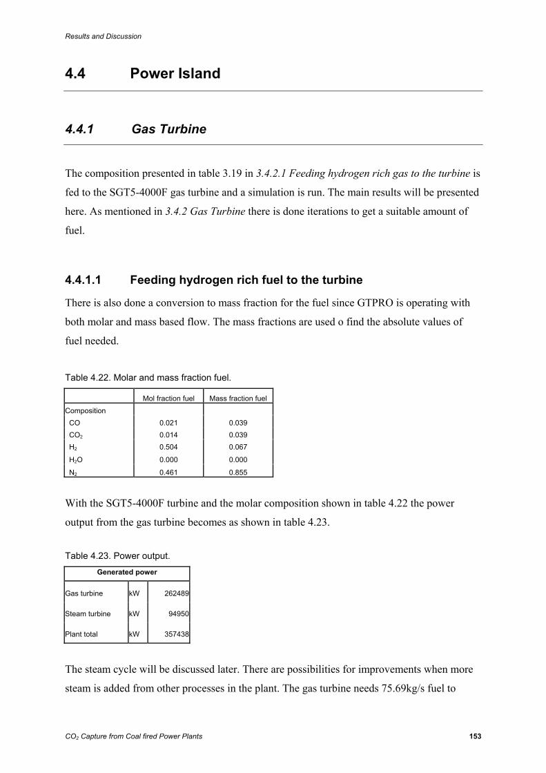
Results and Discussion
CO2 Capture from Coal fired Power Plants 153
4.4 Power Island
4.4.1 Gas Turbine
The composition presented in table 3.19 in 3.4.2.1 Feeding hydrogen rich gas to the turbine is
fed to the SGT5-4000F gas turbine and a simulation is run. The main results will be presented
here. As mentioned in 3.4.2 Gas Turbine there is done iterations to get a suitable amount of
fuel.
4.4.1.1 Feeding hydrogen rich fuel to the turbine
There is also done a conversion to mass fraction for the fuel since GTPRO is operating with
both molar and mass based flow. The mass fractions are used o find the absolute values of
fuel needed.
Table 4.22. Molar and mass fraction fuel.
Mol fraction fuel Mass fraction fuel
Composition CO 0.021 0.039 CO2 0.014 0.039 H2 0.504 0.067
H2O 0.000 0.000
N2 0.461 0.855
With the SGT5-4000F turbine and the molar composition shown in table 4.22 the power
output from the gas turbine becomes as shown in table 4.23.
Table 4.23. Power output. Generated power
Gas turbine kW 262489
Steam turbine kW 94950
Plant total kW 357438
The steam cycle will be discussed later. There are possibilities for improvements when more
steam is added from other processes in the plant. The gas turbine needs 75.69kg/s fuel to

Results and Discussion
CO2 Capture from Coal fired Power Plants 154
produce this amount of power. This is a considerable higher amount than an equal turbine
fired with natural gas. The same turbine fired with pure methane has a methane consumption
of 11.69kg/s. The power output from the gas turbine is however reduced to 212MW because
of the lower mass flow. Methane has a higher specific heating value than the diluted H2 fuel.
Methane has a LHV of 50047kJ/kg and the composition used here has a value of 8453kJ/kg.
That justifies why the fuel amount using this composition is over 6 times higher than for pure
methane. The chemical power input to the gas turbine can be calculated from the mass flow
and the LHV for the fuel.
75.69 8453 639808kg kJ kJs kg s
=i
From this the efficiency for the power island can be calculated. This is so far not that
interesting. Improvements on the steam cycle will increase the power output. In addition is
this an IGCC plant where the chemical energy input to the whole plant is the coal. The coal
goes through energy demanding processes before the power island. All of this has to be
including when calculating overall efficiency. This will be discussed in 4.5 IGCC Power
Plant.
4.4.1.2 Nitrogen, hydrogen and oxygen demand
The chosen gas turbine with the composition given in table 4.22 needs as mentioned a total
fuel amount of 75.69kg/s. By using the total mass flow, the mass fractions and the molar
weight for the substances one could find the demand of N2, H2 and O2 at molar basis. This is
necessary to get the values to fit into the PRO/II simulations. The PRO/II models that is run
so far, calculates with an amount of 1kmol coal. Finding the absolute values of required H2
will give the right amount of coal and then again the right amount of oxygen and steam. The
nitrogen demand for this case is given in equation 4.24.
2
10.855 75.69 2.31028.010
Nkg kmoln
kgs skmol
⎡ ⎤ ⎡ ⎤= =⎢ ⎥ ⎢ ⎥⎡ ⎤⎣ ⎦ ⎣ ⎦⎢ ⎥⎣ ⎦
i i (4.24)
Results and Discussion
CO2 Capture from Coal fired Power Plants 155
Similar for the hydrogen.
2
10.067 75.690 2.5192.016
Hkg kmoln
kgs skmol
⎡ ⎤ ⎡ ⎤= =⎢ ⎥ ⎢ ⎥⎡ ⎤⎣ ⎦ ⎣ ⎦⎢ ⎥⎣ ⎦
i i (4.25)
The amount of H2 calculated her is used to find the right amount of oxygen needed to get this
level of H2 from the Bituminous coal. As shown in the 4.2 Gasification Island, 1kmol of coal
gave 1.031kmol of H2 reacting with 0.28kmol O2. The ratio is then given in 4.26.
2.519 2.4421.031
= (4.26)
This indicates that there is a need 2.442kmol of the chosen coal and 2.442*0.28=0.684 kmol/s
of O2.
From the ASU part there has been found that the 1kmol of air is giving 0.216kmol of O2 and
0.774kmol of N2. Production of 0.684kmol of oxygen will then give
0.684*0.774/0.216=2.450kmol/s of N2. This is a few percent more than the required amount
of 2.310kmol/s. Because of this extra N2 is available from the ASU. There are run simulations
with more N2 in the fuel. This results in a lower turbine inlet temperature and a lower power
output. There is therefore decided to not increase the nitrogen amount even more.
4.4.1.3 Other results from the gas turbine calculations
Other results from the GTPRO simulations are shown in table 4.24.
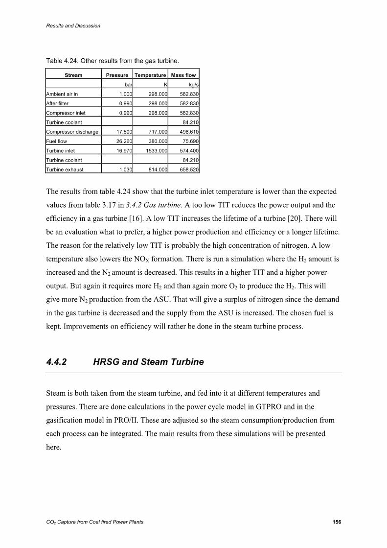
Results and Discussion
CO2 Capture from Coal fired Power Plants 156
Table 4.24. Other results from the gas turbine.
Stream Pressure Temperature Mass flow
bar K kg/s
Ambient air in 1.000 298.000 582.830
After filter 0.990 298.000 582.830
Compressor inlet 0.990 298.000 582.830
Turbine coolant 84.210
Compressor discharge 17.500 717.000 498.610
Fuel flow 26.260 380.000 75.690
Turbine inlet 16.970 1533.000 574.400
Turbine coolant 84.210
Turbine exhaust 1.030 814.000 658.520
The results from table 4.24 show that the turbine inlet temperature is lower than the expected
values from table 3.17 in 3.4.2 Gas turbine. A too low TIT reduces the power output and the
efficiency in a gas turbine [16]. A low TIT increases the lifetime of a turbine [20]. There will
be an evaluation what to prefer, a higher power production and efficiency or a longer lifetime.
The reason for the relatively low TIT is probably the high concentration of nitrogen. A low
temperature also lowers the NOX formation. There is run a simulation where the H2 amount is
increased and the N2 amount is decreased. This results in a higher TIT and a higher power
output. But again it requires more H2 and than again more O2 to produce the H2. This will
give more N2 production from the ASU. That will give a surplus of nitrogen since the demand
in the gas turbine is decreased and the supply from the ASU is increased. The chosen fuel is
kept. Improvements on efficiency will rather be done in the steam turbine process.
4.4.2 HRSG and Steam Turbine
Steam is both taken from the steam turbine, and fed into it at different temperatures and
pressures. There are done calculations in the power cycle model in GTPRO and in the
gasification model in PRO/II. These are adjusted so the steam consumption/production from
each process can be integrated. The main results from these simulations will be presented
here.
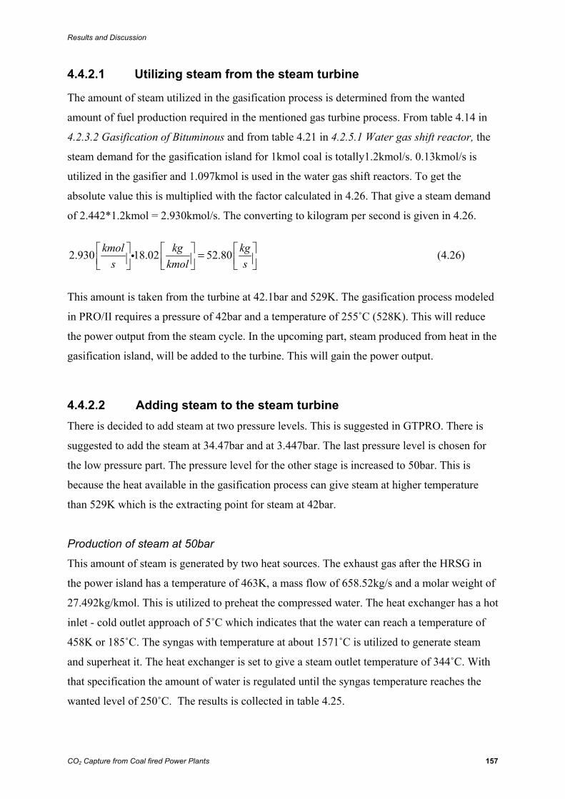
Results and Discussion
CO2 Capture from Coal fired Power Plants 157
4.4.2.1 Utilizing steam from the steam turbine
The amount of steam utilized in the gasification process is determined from the wanted
amount of fuel production required in the mentioned gas turbine process. From table 4.14 in
4.2.3.2 Gasification of Bituminous and from table 4.21 in 4.2.5.1 Water gas shift reactor, the
steam demand for the gasification island for 1kmol coal is totally1.2kmol/s. 0.13kmol/s is
utilized in the gasifier and 1.097kmol is used in the water gas shift reactors. To get the
absolute value this is multiplied with the factor calculated in 4.26. That give a steam demand
of 2.442*1.2kmol = 2.930kmol/s. The converting to kilogram per second is given in 4.26.
2.930 18.02 52.80kmol kg kgs kmol s
⎡ ⎤ ⎡ ⎤ ⎡ ⎤=⎢ ⎥ ⎢ ⎥ ⎢ ⎥⎣ ⎦ ⎣ ⎦ ⎣ ⎦i (4.26)
This amount is taken from the turbine at 42.1bar and 529K. The gasification process modeled
in PRO/II requires a pressure of 42bar and a temperature of 255˚C (528K). This will reduce
the power output from the steam cycle. In the upcoming part, steam produced from heat in the
gasification island, will be added to the turbine. This will gain the power output.
4.4.2.2 Adding steam to the steam turbine There is decided to add steam at two pressure levels. This is suggested in GTPRO. There is
suggested to add the steam at 34.47bar and at 3.447bar. The last pressure level is chosen for
the low pressure part. The pressure level for the other stage is increased to 50bar. This is
because the heat available in the gasification process can give steam at higher temperature
than 529K which is the extracting point for steam at 42bar.
Production of steam at 50bar
This amount of steam is generated by two heat sources. The exhaust gas after the HRSG in
the power island has a temperature of 463K, a mass flow of 658.52kg/s and a molar weight of
27.492kg/kmol. This is utilized to preheat the compressed water. The heat exchanger has a hot
inlet - cold outlet approach of 5˚C which indicates that the water can reach a temperature of
458K or 185˚C. The syngas with temperature at about 1571˚C is utilized to generate steam
and superheat it. The heat exchanger is set to give a steam outlet temperature of 344˚C. With
that specification the amount of water is regulated until the syngas temperature reaches the
wanted level of 250˚C. The results is collected in table 4.25.
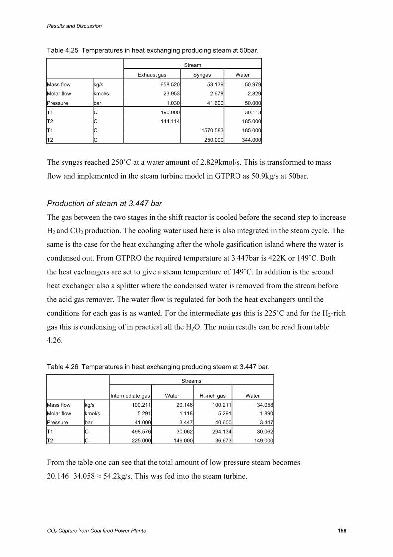
Results and Discussion
CO2 Capture from Coal fired Power Plants 158
Table 4.25. Temperatures in heat exchanging producing steam at 50bar.
Stream Exhaust gas Syngas Water
Mass flow kg/s 658.520 53.139 50.979
Molar flow kmol/s 23.953 2.678 2.829
Pressure bar 1.030 41.600 50.000
T1 C 190.000 30.113
T2 C 144.114 185.000
T1 C 1570.583 185.000
T2 C 250.000 344.000
The syngas reached 250˚C at a water amount of 2.829kmol/s. This is transformed to mass
flow and implemented in the steam turbine model in GTPRO as 50.9kg/s at 50bar.
Production of steam at 3.447 bar
The gas between the two stages in the shift reactor is cooled before the second step to increase
H2 and CO2 production. The cooling water used here is also integrated in the steam cycle. The
same is the case for the heat exchanging after the whole gasification island where the water is
condensed out. From GTPRO the required temperature at 3.447bar is 422K or 149˚C. Both
the heat exchangers are set to give a steam temperature of 149˚C. In addition is the second
heat exchanger also a splitter where the condensed water is removed from the stream before
the acid gas remover. The water flow is regulated for both the heat exchangers until the
conditions for each gas is as wanted. For the intermediate gas this is 225˚C and for the H2-rich
gas this is condensing of in practical all the H2O. The main results can be read from table
4.26.
Table 4.26. Temperatures in heat exchanging producing steam at 3.447 bar.
Streams
Intermediate gas Water H2-rich gas Water
Mass flow kg/s 100.211 20.146 100.211 34.058Molar flow kmol/s 5.291 1.118 5.291 1.890
Pressure bar 41.000 3.447 40.600 3.447
T1 C 498.576 30.062 294.134 30.062
T2 C 225.000 149.000 36.673 149.000
From the table one can see that the total amount of low pressure steam becomes
20.146+34.058 ≈ 54.2kg/s. This was fed into the steam turbine.
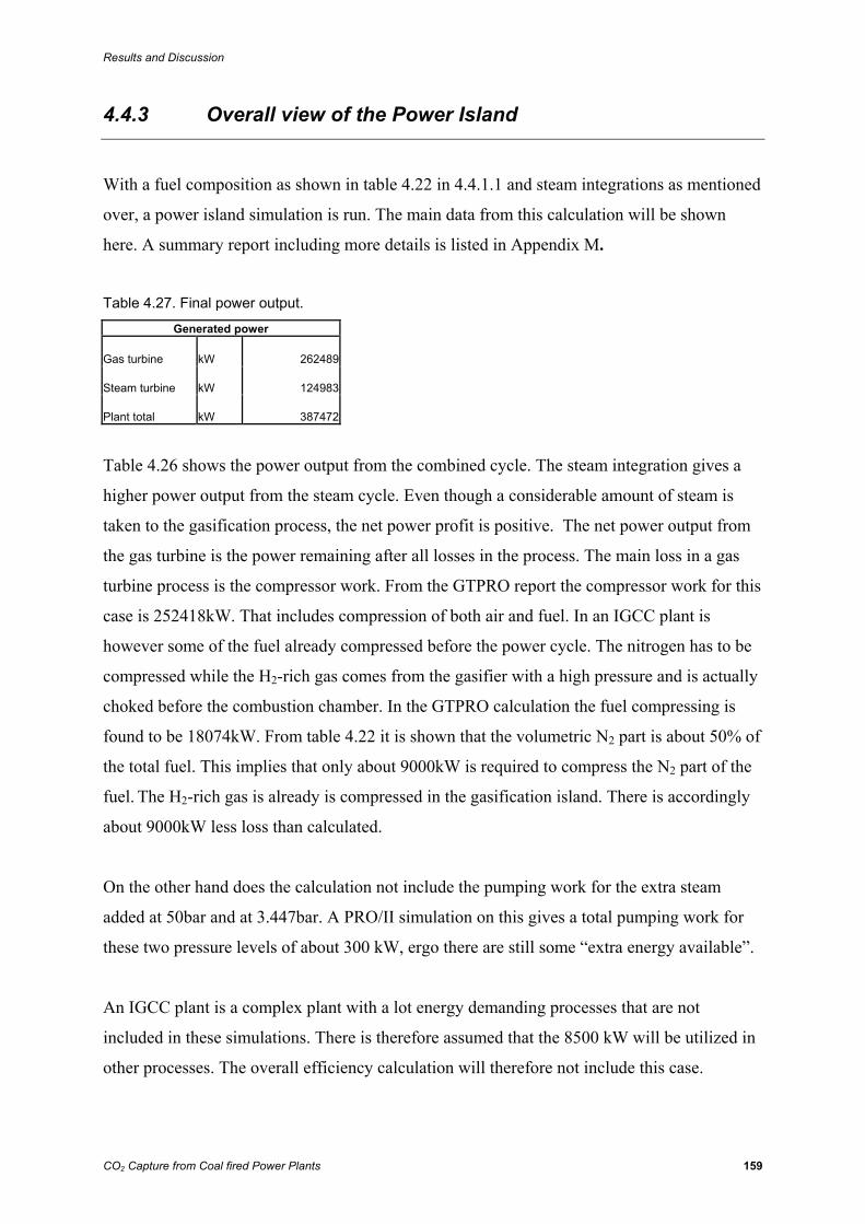
Results and Discussion
CO2 Capture from Coal fired Power Plants 159
4.4.3 Overall view of the Power Island
With a fuel composition as shown in table 4.22 in 4.4.1.1 and steam integrations as mentioned
over, a power island simulation is run. The main data from this calculation will be shown
here. A summary report including more details is listed in Appendix M.
Table 4.27. Final power output.
Generated power
Gas turbine kW 262489
Steam turbine kW 124983
Plant total kW 387472
Table 4.26 shows the power output from the combined cycle. The steam integration gives a
higher power output from the steam cycle. Even though a considerable amount of steam is
taken to the gasification process, the net power profit is positive. The net power output from
the gas turbine is the power remaining after all losses in the process. The main loss in a gas
turbine process is the compressor work. From the GTPRO report the compressor work for this
case is 252418kW. That includes compression of both air and fuel. In an IGCC plant is
however some of the fuel already compressed before the power cycle. The nitrogen has to be
compressed while the H2-rich gas comes from the gasifier with a high pressure and is actually
choked before the combustion chamber. In the GTPRO calculation the fuel compressing is
found to be 18074kW. From table 4.22 it is shown that the volumetric N2 part is about 50% of
the total fuel. This implies that only about 9000kW is required to compress the N2 part of the
fuel. The H2-rich gas is already is compressed in the gasification island. There is accordingly
about 9000kW less loss than calculated.
On the other hand does the calculation not include the pumping work for the extra steam
added at 50bar and at 3.447bar. A PRO/II simulation on this gives a total pumping work for
these two pressure levels of about 300 kW, ergo there are still some “extra energy available”.
An IGCC plant is a complex plant with a lot energy demanding processes that are not
included in these simulations. There is therefore assumed that the 8500 kW will be utilized in
other processes. The overall efficiency calculation will therefore not include this case.
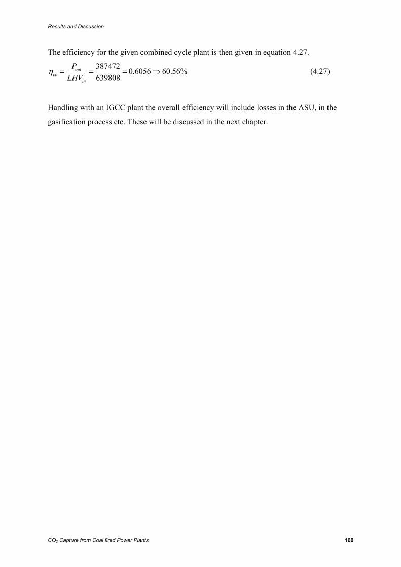
Results and Discussion
CO2 Capture from Coal fired Power Plants 160
The efficiency for the given combined cycle plant is then given in equation 4.27.
387472 0.6056 60.56%639808
outcc
in
PLHV
η = = = ⇒ (4.27)
Handling with an IGCC plant the overall efficiency will include losses in the ASU, in the
gasification process etc. These will be discussed in the next chapter.
Results and Discussion
CO2 Capture from Coal fired Power Plants 161
4.5 IGCC Power Plant
4.5.1 Initial calculation
The main numbers of the different islands is collected and set together in an Excel sheet. The
feed to the gasifier is adjusted from the feed needed to the turbine in GTPRO. The feed to the
ASU is again adjusted from the need in the gasifier. 96% of the CO2 is removed after the shift
reactor.
With the numbers given in the previous sections of 4 Results and Discussion the following
Excel sheet gives the overall plant calculations.
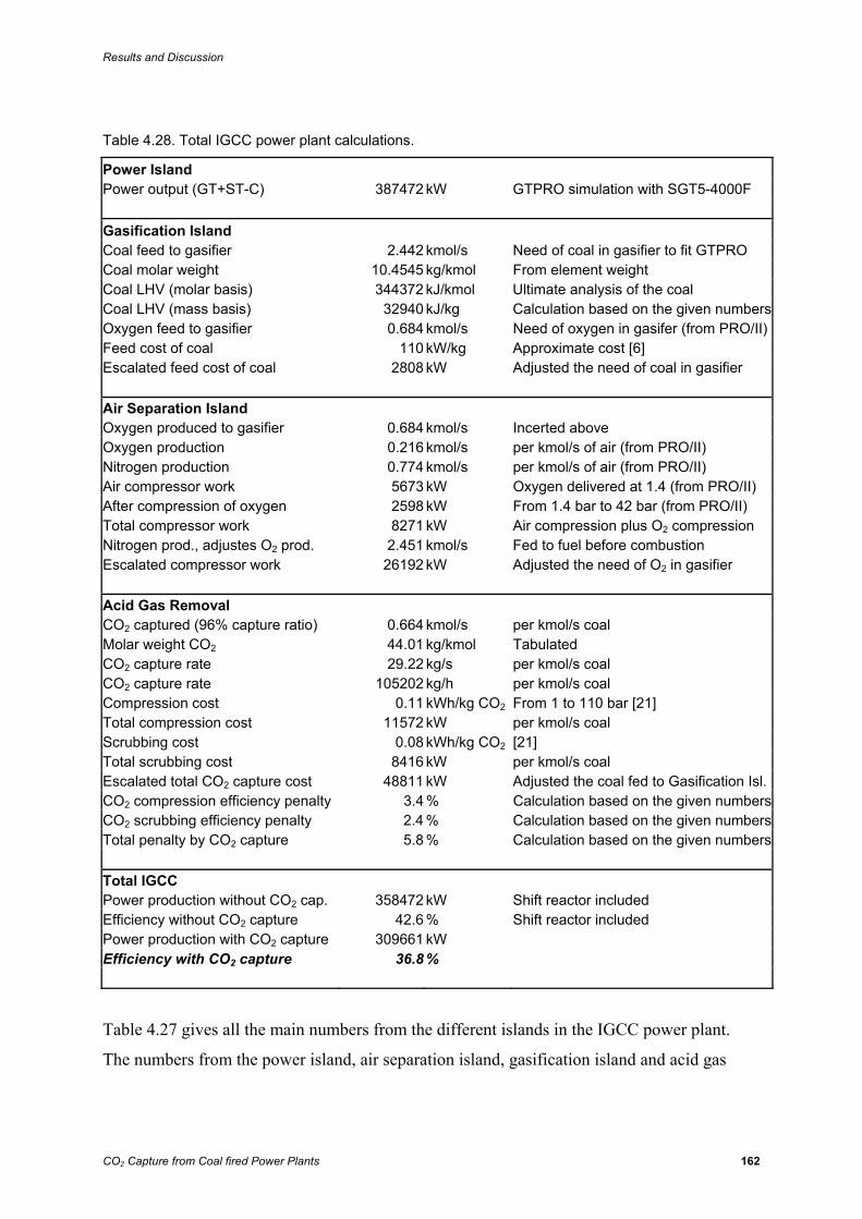
Results and Discussion
CO2 Capture from Coal fired Power Plants 162
Table 4.28. Total IGCC power plant calculations.
Power Island Power output (GT+ST-C) 387472 kW GTPRO simulation with SGT5-4000F Gasification Island Coal feed to gasifier 2.442 kmol/s Need of coal in gasifier to fit GTPRO Coal molar weight 10.4545 kg/kmol From element weight Coal LHV (molar basis) 344372 kJ/kmol Ultimate analysis of the coal Coal LHV (mass basis) 32940 kJ/kg Calculation based on the given numbersOxygen feed to gasifier 0.684 kmol/s Need of oxygen in gasifer (from PRO/II)Feed cost of coal 110 kW/kg Approximate cost [6] Escalated feed cost of coal 2808 kW Adjusted the need of coal in gasifier Air Separation Island Oxygen produced to gasifier 0.684 kmol/s Incerted above Oxygen production 0.216 kmol/s per kmol/s of air (from PRO/II) Nitrogen production 0.774 kmol/s per kmol/s of air (from PRO/II) Air compressor work 5673 kW Oxygen delivered at 1.4 (from PRO/II) After compression of oxygen 2598 kW From 1.4 bar to 42 bar (from PRO/II) Total compressor work 8271 kW Air compression plus O2 compression Nitrogen prod., adjustes O2 prod. 2.451 kmol/s Fed to fuel before combustion Escalated compressor work 26192 kW Adjusted the need of O2 in gasifier Acid Gas Removal CO2 captured (96% capture ratio) 0.664 kmol/s per kmol/s coal Molar weight CO2 44.01 kg/kmol Tabulated CO2 capture rate 29.22 kg/s per kmol/s coal CO2 capture rate 105202 kg/h per kmol/s coal Compression cost 0.11 kWh/kg CO2 From 1 to 110 bar [21] Total compression cost 11572 kW per kmol/s coal Scrubbing cost 0.08 kWh/kg CO2 [21] Total scrubbing cost 8416 kW per kmol/s coal Escalated total CO2 capture cost 48811 kW Adjusted the coal fed to Gasification Isl.CO2 compression efficiency penalty 3.4 % Calculation based on the given numbersCO2 scrubbing efficiency penalty 2.4 % Calculation based on the given numbersTotal penalty by CO2 capture 5.8 % Calculation based on the given numbers Total IGCC Power production without CO2 cap. 358472 kW Shift reactor included Efficiency without CO2 capture 42.6 % Shift reactor included Power production with CO2 capture 309661 kW Efficiency with CO2 capture 36.8 %
Table 4.27 gives all the main numbers from the different islands in the IGCC power plant.
The numbers from the power island, air separation island, gasification island and acid gas
Results and Discussion
CO2 Capture from Coal fired Power Plants 163
removal is discussed and presented in the previous sections of 4 Results and discussion and
will not be discussed particularly in this part of the report.
The most important numbers presented here are the efficiencies of the modeled plant. The
overall efficiency without CO2 capture is 42.6%. This number is although not particularly
interesting due to the implemented shift reactor. An IGCC plant without CO2 capture would
not have a shift reactor included in the gasification island like this model has. The H2 and CO
rich syngas would be used directly as fuel gas and the efficiency would be higher.
The efficiency when carbon dioxide capture is included is very interesting. This number
includes the losses by production and compression of oxygen and nitrogen, the coal feed cost,
the production of high pressure steam to the gasifier and shift reactor, the removal and
compression of CO2 and pressure losses through the plant. An efficiency included CO2
capture of 36.8% is a very satisfying result.
There are probably other losses not considered in this model. A real life power plant is also
much more complex and advanced than a computer model. Complexity and units not
considered in this model will probably reduce the efficiency. From 4.2.3.4 Comparison the
amount of produced syngas is calculated to be a bit higher than expected from literature. This
will contribute to a higher overall efficiency. A lower production rate will decrease the
efficiency. The efficiency of 36.8 percent is although very good and even with a reduction of
2-3 percentage points, the efficiency would still be satisfying.
4.5.2 Deviation from initial calculation
The numbers and efficiencies collected from the different islands are based on some initial
assumptions. If these assumptions are changed it could have favourable impact on the total
efficiency.
As mentioned in 4.1.1.6 Overall GOX considerations the polytrophic compressor efficiency
in the air separation unit is sometimes assumed to be 90% instead of 85%. If the total IGCC
plant calculations are performed with this assumption the efficiency with CO2 capture is
increased to 37.0%. An increase of 0.2 percentage points is not remarkable, but investing in
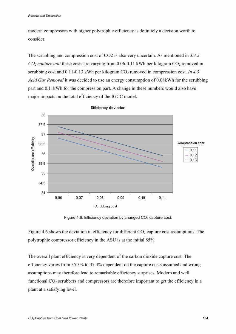
Results and Discussion
CO2 Capture from Coal fired Power Plants 164
modern compressors with higher polytrophic efficiency is definitely a decision worth to
consider.
The scrubbing and compression cost of CO2 is also very uncertain. As mentioned in 3.3.2
CO2 capture unit these costs are varying from 0.06-0.11 kWh per kilogram CO2 removed in
scrubbing cost and 0.11-0.13 kWh per kilogram CO2 removed in compression cost. In 4.3
Acid Gas Removal it was decided to use an energy consumption of 0.08kWh for the scrubbing
part and 0.11kWh for the compression part. A change in these numbers would also have
major impacts on the total efficiency of the IGCC model.
Figure 4.6. Efficiency deviation by changed CO2 capture cost.
Figure 4.6 shows the deviation in efficiency for different CO2 capture cost assumptions. The
polytrophic compressor efficiency in the ASU is at the initial 85%.
The overall plant efficiency is very dependent of the carbon dioxide capture cost. The
efficiency varies from 35.3% to 37.4% dependent on the capture costs assumed and wrong
assumptions may therefore lead to remarkable efficiency surprises. Modern and well
functional CO2 scrubbers and compressors are therefore important to get the efficiency in a
plant at a satisfying level.
Results and Discussion
CO2 Capture from Coal fired Power Plants 165
4.5.3 Main numbers in favourable units
Through the report the production rates of the islands have mainly been describes in kmol/s.
For simulations and integration between computer tools this is a favourable measure unit. The
production rates of plants are although often referred in more understandable units as normal
cubic meters per second (Nm3) or tons per day (tons/day).
The numbers presented in this section is fitted the GTPRO simulation of 387472kW which
equals about 387MW. This is only the GTPRO simulation and integrated with the other
islands the output of the total plant is at about 310MW.
To produce the mentioned amount of electricity the Gasification Island must produce 59.6
Nm3/s of H2 rich gas. Per day this equals about 5.15 million Nm3.
The production demand in the Gasification Island to fit the GTPRO simulation requires
2.442kmol/s of the given coal type. This equals about 2206tons/day.
To gasify this amount of coal it is needed 0.684kmol/s of oxygen produced in the Air
Separation Island. 0.684kmol/s corresponds to 16.2 Nm3/s or 1891tons/day.
Conclusion
CO2 Capture from Coal fired Power Plants 166
5 Conclusion
Coal is the most common source for electricity production globally. The demand of power is
increasing and new coal fired power plants are built continuous. IGCC is a technology giving
incentives to CO2 capture from coal fired power plants.
Integrated Gasification Combined Cycle consists of four main processes set together in a total
IGCC power plant. The air separator produces oxygen which is fed to the gasification island
together with steam and coal. In the gasifier coal is transformed to syngas consisting of
mainly hydrogen and carbon monoxide. To be able to capture CO2, the CO is reacted with
steam in a shift reactor producing H2 and CO2. Carbon dioxide is removed by physical
absorption before the H2 rich fuel gas is diluted with nitrogen from the ASU and sent to the
combustion chamber.
The air separation unit was modeled in PRO/II which is an excellent tool for cryogenic
distillation. Under the given assumptions the ASU produces oxygen at an energy cost of
0.238kWh per kilogram pure oxygen delivered at 25°C and 1.4bar. The waste nitrogen is
mainly utilized as diluter in the fuel gas. The products have a purity level at 95.6% for the
oxygen and 99.6% for the nitrogen. Compared to industry standard both the energy
consumption and product qualities are at satisfying levels.
The gasification island was also modeled in PRO/II. The program is not designed for solid
fuels, but was verified as a proper tool for molar balance calculations. Comparison between
PRO/II and results from an equilibrium calculator programmed in MatLab in addition to
empirical data from a commercial entrained flow gasifier gave similar syngas compositions.
The gasifier modeled has a Cold Gas Efficiency of 84.0% which is above the demand of a
minimum of 78% to consider gasification feasible.
The acid gas removal is not modeled. A physical absorption process with selexol as solvent is
reported to have a scrubber energy cost of 0.06-0.11kWh per kilogram CO2 captured. In
addition a compression cost of 0.11-0.13kWh per kilogram CO2 must be included in the
calculation. It is assumed a scrubber cost of 0.08 and a compression cost of 0.11kWh per kg
CO2 removed. Deviation in the assumed capture costs may change the calculated overall plant

Conclusion
CO2 Capture from Coal fired Power Plants 167
efficiency with 1-2 percentage points. The CO2 scrubber has a capture ratio of 96% and do
also remove H2S and other unwanted minor substances.
The power island is modeled in GTPRO which is a good tool for almost every power
calculations. GTPRO is also able to model the gasification island, but this is as mentioned
done in PRO/II. CO2 and H2S are removed from the fuel gas and nitrogen is added in an Excel
sheet. In GTPRO a turbine able to handle large amounts of H2 is chosen. The HRSG is
integrated with the syngas cooler and produces steam to the gasification island in PRO/II.
Data from the four main processes are collected in an Excel sheet calculating the total
efficiency of the plant. The overall efficiency of the IGCC power plant model ended at 36.8%.
This number includes the losses by production and compression of oxygen and nitrogen, the
coal feed cost, the production of high pressure steam to the gasifier and shift reactor, the
removal and compression of CO2 and pressure losses through the plant. The result is very
satisfying compared to reports based on similar models.
In other models and in real life there might be units and losses not considered in this model.
Changes in the assumptions may give great changes in the efficiency and should always be
very well discussed.
Reference List
CO2 Capture from Coal fired Power Plants 168
6 Reference List
[1] The United Nations Framework Convention on Climate Change (UNFCCC),
1997. Article 2: Objective [online]. Available from:
http://unfccc.int/essential_background/convention/background/items/1353.php
[Accessed 13 Nov 2007].
[2] Metz, B., Davidson, O., de Coninck, H., Loos, M. and Meyer L. IPCC Special Report
on Carbon Dioxide Capture and Storage. New York: Cambridge University Press,
2005.
[3] Naqvi, R., Natural Gas Power with CO2 Treatment. Paper presented in lecture in
TPG4140 Natural Gas, Trondheim, 3 Oct 2006.
[4] Bolland, O. CO2 Capture. Paper presented in lecture in TEP03 Turbomachinery and
Power Production, Trondheim, 15 Nov 2007.
[5] British Petroleum (BP), 2007. Statistical Review charting tool [online].
Available from: http://www.investis.com/bp_acc_ia/stat_review_06/htdocs/index.html
[Accessed 12 Dec 2007]
[6] Higman, C. and van der Burgt, M., Gasification. Burlington: Gulf Professional
Publishing/Elsevier, 2003.
[7] Allam, R.J., Improved Oxygen Production Technologies. (Report to International
Energy Agency Greenhouse Gas R&D Programme (IEA GHG), 2007)
[8] Humphrey, J.L., Keller II, G.E., Separation Process Technologies, New York:
McGraw-Hill, 1997.
[9] Geankoplis, C.J., Transport Processes and Unit Operations, Prentice Hall, 1983.
[10] Bolland, O., Personal conversation, autumn 2007 and spring 2008.
Reference List
CO2 Capture from Coal fired Power Plants 169
[11] Anantharaman, R., Personal conversation, spring 2008.
[12] Lide, D.R., CRC Handbook of Chemistry and Physics, Taylor and Francis Group
LLC, 1997.
[13] Airliquide, Gas Encyclopaedia [online], Available from:
http://encyclopedia.airliquide.com/encyclopedia.asp?CountryID=19&LanguageID=11
[Accessed 12 Mar 2008]
[14] Universal Industrial Gases Inc, Overview of Cryogenic Air Separation and Liquefier
Systems [online], Available from: www.uigi.com/cryodist.html
[Accessed 12 Mar 2008]
[15] Gundersen, T., TEP4215 Process Integration, Lecture notes presented spring 2007.
[16] Bolland, O., Thermal power generation. Compendium presented in TEP03
Turbomachinery and Power Production, Trondheim, autumn 2007.
[17] World Coal Institute, 2007. Coal Facts 2007 [online]. Available from:
http://www.worldcoal.org/pages/content/index.asp?PageID=188
[Accessed 12 Dec 2007].
[18] Probstein, R.F. and Hicks R.E., Synthetic Fuels. Mineola: Dover Publications,
Inc., 2006.
[19] Moran, M.J., Shapiro, H.N., Fundamentals of Engineering Thermodynamics. New
Jersey: John Wiley & Sons, Inc., 2004.
[20] Maurstad, O., An overview of Coal based Integrated Gasification Combined Cycle
(IGCC) Technology, (Publication No. LFEE 2005-002 WP, 2005, Laboratory for
Energy and the Environment, Massachusetts Institute of Technology)
Reference List
CO2 Capture from Coal fired Power Plants 170
[21] Göttlicher, G, The Energetics of Carbon Dioxide Capture in Power Plants. (VDI
Progress Reports Series 6 No. 421, 1999)
[22] Sulfotech Research., Converting Hydrogen Sulfide by the Claus Process [online],
Available from: http://www.nelliott.demon.co.uk/company/claus.html
[Accessed 24 Jun 2008]
[23] Saravanamuttoo, H.I.H., Rogers, G.F.C., Cohen, H., Gas Turbine Theory, Essex:
Pearson Education Limited, 2001.
[24] Siemens Power Generation, 2007, Siemens Gas Turbine H2 Combustion Technology
for Low Carbon IGCC [online], Available from:
http://www.gasification.org/Docs/2007_Papers/29BROW.pdf
[Accessed 05 May 2008]
[25] Smith, R., Chemical Process Design and Integration, West Sussex: John Wiley and
Sons Ltd, 2005.
[26] Colorado State University, Chemical Equilibrium Calculation [online],
Available from: http://navier.engr.colostate.edu/tools/equil.html
[Accessed 12 Feb 2008]
[27] Ertesvåg, I.S., Personal conversation, spring 2008.
Appendix
CO2 Capture from Coal fired Power Plants 171
Appendix Index
Appendix A Chemical equilibrium derivation……………………………………...……..172
Appendix B MatLab fsolve function……………………………………………………...174
Appendix C MatLab run fsolve function……………………………………………….....176
Appendix D Coal as gas compared with chosen coal composition……………………….177
Appendix E Stream properties for initial GOX…………………………………………...180
Appendix F Stream and compressor properties for improved CCR………………………181
Appendix G Stream properties for modifications in the main heat exchanger……………183
Appendix H Number of compressor in ASU model……………………………………....185
Appendix I Stream properties for minimum number of trays……………………..……..188
Appendix J Properties for the optimal GOX model……………………………..……….189
Appendix K Stream properties LOX………………………………………………………192
Appendix L Chemical calculator example……………………………………………..…194
Appendix M GTPRO simulation example………………………………………………....195
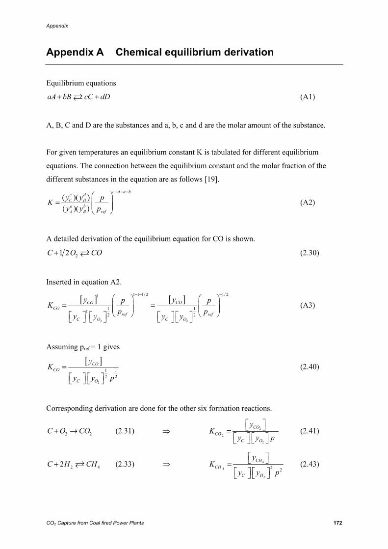
Appendix
CO2 Capture from Coal fired Power Plants 172
Appendix A Chemical equilibrium derivation
Equilibrium equations
aA bB cC dD+ + (A1)
A, B, C and D are the substances and a, b, c and d are the molar amount of the substance.
For given temperatures an equilibrium constant K is tabulated for different equilibrium
equations. The connection between the equilibrium constant and the molar fraction of the
different substances in the equation are as follows [19].
( )( )( )( )
c d a bc dC Da bA B ref
y y pKy y p
+ − −⎛ ⎞
= ⎜ ⎟⎜ ⎟⎝ ⎠
(A2)
A detailed derivation of the equilibrium equation for CO is shown.
21 2C O CO+ (2.30)
Inserted in equation A2.
[ ] [ ]
2 2
1 1 1/ 2 1/ 21
1 112 2
CO COCO
ref refC O C O
y yp pKp py y y y
− − −⎛ ⎞ ⎛ ⎞
= =⎜ ⎟ ⎜ ⎟⎜ ⎟ ⎜ ⎟⎝ ⎠ ⎝ ⎠⎡ ⎤ ⎡ ⎤ ⎡ ⎤ ⎡ ⎤⎣ ⎦ ⎣ ⎦ ⎣ ⎦ ⎣ ⎦
(A3)
Assuming pref = 1 gives
[ ]
2
1122
COCO
C O
yK
y y p=⎡ ⎤ ⎡ ⎤⎣ ⎦ ⎣ ⎦
(2.40)
Corresponding derivation are done for the other six formation reactions.
2 2C O CO+ → (2.31) ⇒ 2
2
2
COCO
C O
yK
y y p
⎡ ⎤⎣ ⎦=⎡ ⎤ ⎡ ⎤⎣ ⎦ ⎣ ⎦
(2.41)
2 42C H CH+ (2.33) ⇒ 4
4
2
2 2
CHCH
C H
yK
y y p
⎡ ⎤⎣ ⎦=⎡ ⎤ ⎡ ⎤⎣ ⎦ ⎣ ⎦
(2.43)
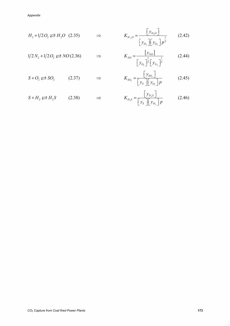
Appendix
CO2 Capture from Coal fired Power Plants 173
2 2 21 2H O H O+ (2.35) ⇒ 2
2
2 2
12
H OH O
H O
yK
y y p
⎡ ⎤⎣ ⎦=⎡ ⎤ ⎡ ⎤⎣ ⎦ ⎣ ⎦
(2.42)
2 21 2 1 2N O NO+ (2.36) ⇒ [ ]
2 2
1 12 2
NONO
O N
yK
y y=⎡ ⎤ ⎡ ⎤⎣ ⎦ ⎣ ⎦
(2.44)
2 2S O SO+ (2.37) ⇒ 2
2
2
SOSO
S O
yK
y y p
⎡ ⎤⎣ ⎦=⎡ ⎤ ⎡ ⎤⎣ ⎦ ⎣ ⎦
(2.45)
2 2S H H S+ (2.38) ⇒ 2
2
2
H SH S
S H
yK
y y p
⎡ ⎤⎣ ⎦=⎡ ⎤ ⎡ ⎤⎣ ⎦ ⎣ ⎦
(2.46)
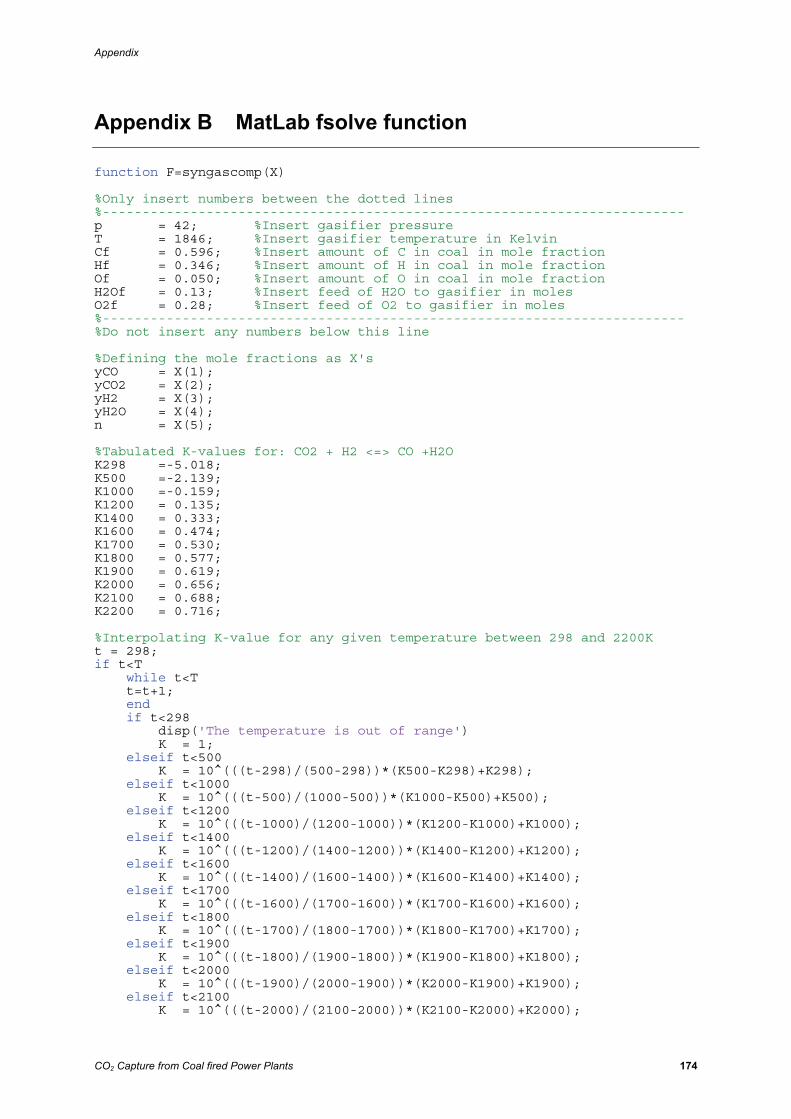
Appendix
CO2 Capture from Coal fired Power Plants 174
Appendix B MatLab fsolve function function F=syngascomp(X) %Only insert numbers between the dotted lines %------------------------------------------------------------------------- p = 42; %Insert gasifier pressure T = 1846; %Insert gasifier temperature in Kelvin Cf = 0.596; %Insert amount of C in coal in mole fraction Hf = 0.346; %Insert amount of H in coal in mole fraction Of = 0.050; %Insert amount of O in coal in mole fraction H2Of = 0.13; %Insert feed of H2O to gasifier in moles O2f = 0.28; %Insert feed of O2 to gasifier in moles %------------------------------------------------------------------------- %Do not insert any numbers below this line %Defining the mole fractions as X's yCO = X(1); yCO2 = X(2); yH2 = X(3); yH2O = X(4); n = X(5); %Tabulated K-values for: CO2 + H2 <=> CO +H2O K298 =-5.018; K500 =-2.139; K1000 =-0.159; K1200 = 0.135; K1400 = 0.333; K1600 = 0.474; K1700 = 0.530; K1800 = 0.577; K1900 = 0.619; K2000 = 0.656; K2100 = 0.688; K2200 = 0.716; %Interpolating K-value for any given temperature between 298 and 2200K t = 298; if t<T while t<T t=t+1; end if t<298 disp('The temperature is out of range') K = 1; elseif t<500 K = 10^(((t-298)/(500-298))*(K500-K298)+K298); elseif t<1000 K = 10^(((t-500)/(1000-500))*(K1000-K500)+K500); elseif t<1200 K = 10^(((t-1000)/(1200-1000))*(K1200-K1000)+K1000); elseif t<1400 K = 10^(((t-1200)/(1400-1200))*(K1400-K1200)+K1200); elseif t<1600 K = 10^(((t-1400)/(1600-1400))*(K1600-K1400)+K1400); elseif t<1700 K = 10^(((t-1600)/(1700-1600))*(K1700-K1600)+K1600); elseif t<1800 K = 10^(((t-1700)/(1800-1700))*(K1800-K1700)+K1700); elseif t<1900 K = 10^(((t-1800)/(1900-1800))*(K1900-K1800)+K1800); elseif t<2000 K = 10^(((t-1900)/(2000-1900))*(K2000-K1900)+K1900); elseif t<2100 K = 10^(((t-2000)/(2100-2000))*(K2100-K2000)+K2000);
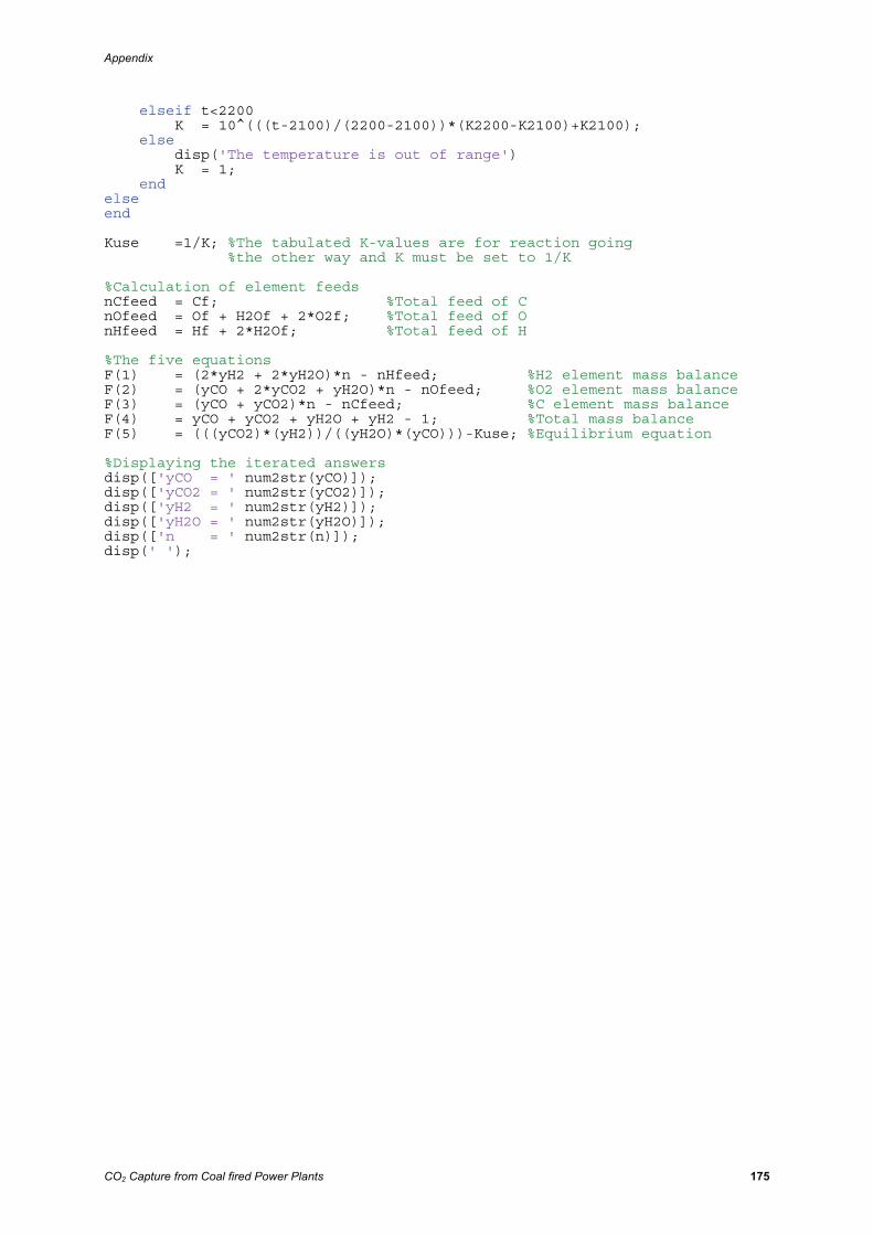
Appendix
CO2 Capture from Coal fired Power Plants 175
elseif t<2200 K = 10^(((t-2100)/(2200-2100))*(K2200-K2100)+K2100); else disp('The temperature is out of range') K = 1; end else end Kuse =1/K; %The tabulated K-values are for reaction going %the other way and K must be set to 1/K %Calculation of element feeds nCfeed = Cf; %Total feed of C nOfeed = Of + H2Of + 2*O2f; %Total feed of O nHfeed = Hf + 2*H2Of; %Total feed of H %The five equations F(1) = (2*yH2 + 2*yH2O)*n - nHfeed; %H2 element mass balance F(2) = (yCO + 2*yCO2 + yH2O)*n - nOfeed; %O2 element mass balance F(3) = (yCO + yCO2)*n - nCfeed; %C element mass balance F(4) = yCO + yCO2 + yH2O + yH2 - 1; %Total mass balance F(5) = (((yCO2)*(yH2))/((yH2O)*(yCO)))-Kuse; %Equilibrium equation %Displaying the iterated answers disp(['yCO = ' num2str(yCO)]); disp(['yCO2 = ' num2str(yCO2)]); disp(['yH2 = ' num2str(yH2)]); disp(['yH2O = ' num2str(yH2O)]); disp(['n = ' num2str(n)]); disp(' ');

Appendix
CO2 Capture from Coal fired Power Plants 176
Appendix C MatLab run fsolve function %Programname: calculatesyngas %The script runs the fsolve function for syngascomp %Start values for the composition yCO = 0.5; yCO2 = 0.5; yH2 = 0.5; yH2O = 0.5; n = 1.2; fsolve('syngascomp',[yCO yCO2 yH2 yH2O n]);
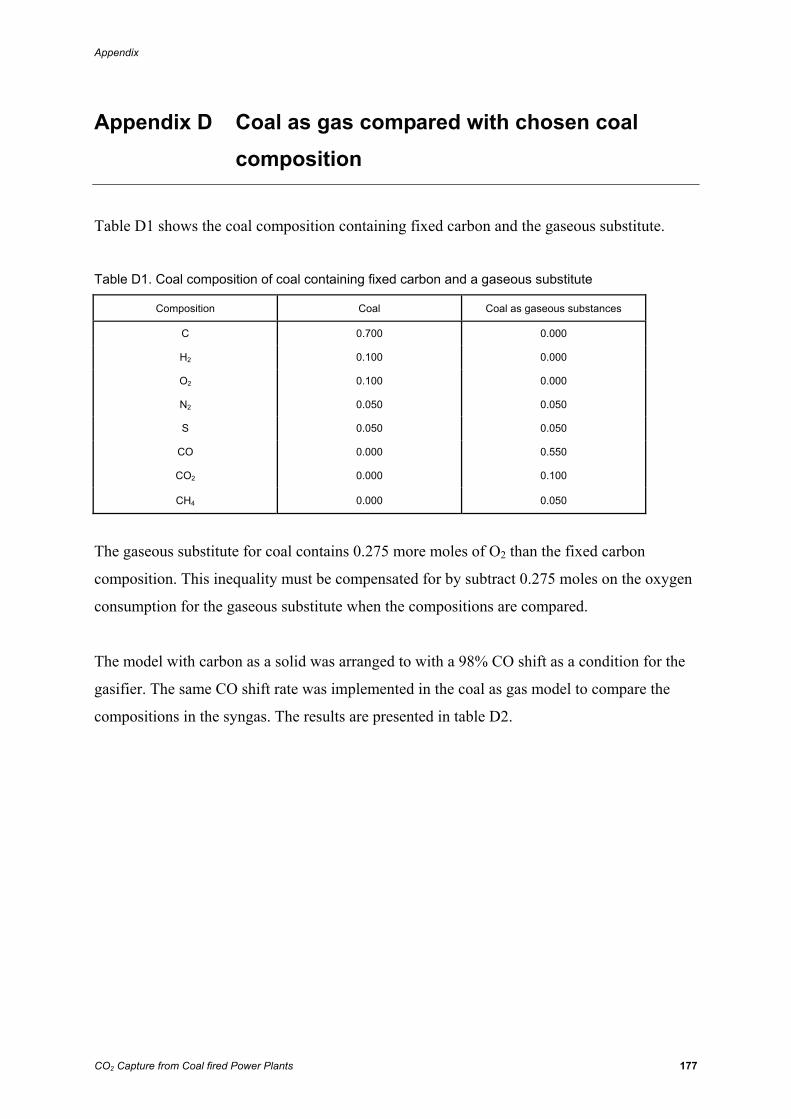
Appendix
CO2 Capture from Coal fired Power Plants 177
Appendix D Coal as gas compared with chosen coal composition
Table D1 shows the coal composition containing fixed carbon and the gaseous substitute.
Table D1. Coal composition of coal containing fixed carbon and a gaseous substitute
Composition Coal Coal as gaseous substances
C 0.700 0.000
H2 0.100 0.000
O2 0.100 0.000
N2 0.050 0.050
S 0.050 0.050
CO 0.000 0.550
CO2 0.000 0.100
CH4 0.000 0.050
The gaseous substitute for coal contains 0.275 more moles of O2 than the fixed carbon
composition. This inequality must be compensated for by subtract 0.275 moles on the oxygen
consumption for the gaseous substitute when the compositions are compared.
The model with carbon as a solid was arranged to with a 98% CO shift as a condition for the
gasifier. The same CO shift rate was implemented in the coal as gas model to compare the
compositions in the syngas. The results are presented in table D2.
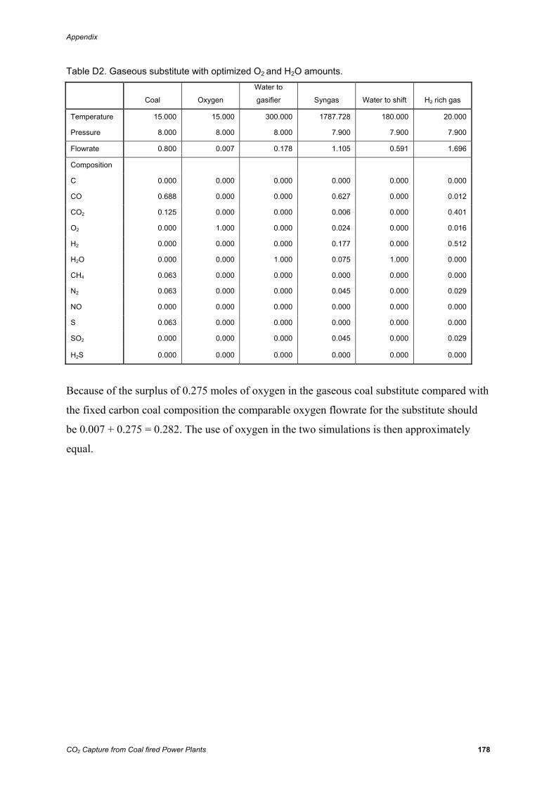
Appendix
CO2 Capture from Coal fired Power Plants 178
Table D2. Gaseous substitute with optimized O2 and H2O amounts.
Coal Oxygen
Water to
gasifier Syngas Water to shift H2 rich gas
Temperature 15.000 15.000 300.000 1787.728 180.000 20.000
Pressure 8.000 8.000 8.000 7.900 7.900 7.900
Flowrate 0.800 0.007 0.178 1.105 0.591 1.696
Composition
C 0.000 0.000 0.000 0.000 0.000 0.000
CO 0.688 0.000 0.000 0.627 0.000 0.012
CO2 0.125 0.000 0.000 0.006 0.000 0.401
O2 0.000 1.000 0.000 0.024 0.000 0.016
H2 0.000 0.000 0.000 0.177 0.000 0.512
H2O 0.000 0.000 1.000 0.075 1.000 0.000
CH4 0.063 0.000 0.000 0.000 0.000 0.000
N2 0.063 0.000 0.000 0.045 0.000 0.029
NO 0.000 0.000 0.000 0.000 0.000 0.000
S 0.063 0.000 0.000 0.000 0.000 0.000
SO2 0.000 0.000 0.000 0.045 0.000 0.029
H2S 0.000 0.000 0.000 0.000 0.000 0.000
Because of the surplus of 0.275 moles of oxygen in the gaseous coal substitute compared with
the fixed carbon coal composition the comparable oxygen flowrate for the substitute should
be 0.007 + 0.275 = 0.282. The use of oxygen in the two simulations is then approximately
equal.
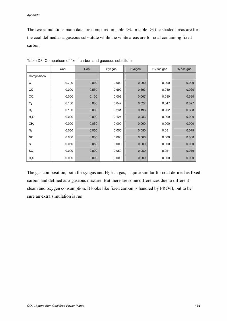
Appendix
CO2 Capture from Coal fired Power Plants 179
The two simulations main data are compared in table D3. In table D3 the shaded areas are for
the coal defined as a gaseous substitute while the white areas are for coal containing fixed
carbon
Table D3. Comparison of fixed carbon and gaseous substitute.
Coal Coal Syngas Syngas H2 rich gas H2 rich gas
Composition
C 0.700 0.000 0.000 0.000 0.000 0.000
CO 0.000 0.550 0.692 0.693 0.019 0.020
CO2 0.000 0.100 0.008 0.007 0.680 0.680
O2 0.100 0.000 0.047 0.027 0.047 0.027
H2 0.100 0.000 0.231 0.196 0.902 0.868
H2O 0.000 0.000 0.124 0.083 0.000 0.000
CH4 0.000 0.050 0.000 0.000 0.000 0.000
N2 0.050 0.050 0.050 0.050 0.051 0.049
NO 0.000 0.000 0.000 0.000 0.000 0.000
S 0.050 0.050 0.000 0.000 0.000 0.000
SO2 0.000 0.000 0.050 0.050 0.051 0.049
H2S 0.000 0.000 0.000 0.000 0.000 0.000
The gas composition, both for syngas and H2 rich gas, is quite similar for coal defined as fixed
carbon and defined as a gaseous mixture. But there are some differences due to different
steam and oxygen consumption. It looks like fixed carbon is handled by PRO/II, but to be
sure an extra simulation is run.
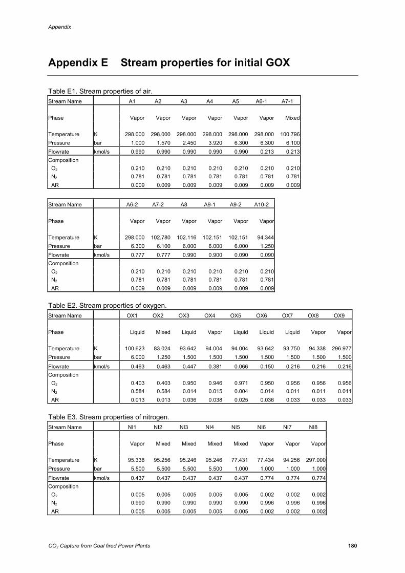
Appendix
CO2 Capture from Coal fired Power Plants 180
Appendix E Stream properties for initial GOX
Table E1. Stream properties of air. Stream Name A1 A2 A3 A4 A5 A6-1 A7-1 Phase Vapor Vapor Vapor Vapor Vapor Vapor Mixed Temperature K 298.000 298.000 298.000 298.000 298.000 298.000 100.796 Pressure bar 1.000 1.570 2.450 3.920 6.300 6.300 6.100 Flowrate kmol/s 0.990 0.990 0.990 0.990 0.990 0.213 0.213 Composition O2 0.210 0.210 0.210 0.210 0.210 0.210 0.210 N2 0.781 0.781 0.781 0.781 0.781 0.781 0.781 AR 0.009 0.009 0.009 0.009 0.009 0.009 0.009
Stream Name A6-2 A7-2 A8 A9-1 A9-2 A10-2 Phase Vapor Vapor Vapor Vapor Vapor Vapor Temperature K 298.000 102.780 102.116 102.151 102.151 94.344Pressure bar 6.300 6.100 6.000 6.000 6.000 1.250Flowrate kmol/s 0.777 0.777 0.990 0.900 0.090 0.090Composition O2 0.210 0.210 0.210 0.210 0.210 0.210 N2 0.781 0.781 0.781 0.781 0.781 0.781 AR 0.009 0.009 0.009 0.009 0.009 0.009
Table E2. Stream properties of oxygen. Stream Name OX1 OX2 OX3 OX4 OX5 OX6 OX7 OX8 OX9 Phase Liquid Mixed Liquid Vapor Liquid Liquid Liquid Vapor Vapor Temperature K 100.623 83.024 93.642 94.004 94.004 93.642 93.750 94.338 296.977Pressure bar 6.000 1.250 1.500 1.500 1.500 1.500 1.500 1.500 1.500
Flowrate kmol/s 0.463 0.463 0.447 0.381 0.066 0.150 0.216 0.216 0.216Composition O2 0.403 0.403 0.950 0.946 0.971 0.950 0.956 0.956 0.956 N2 0.584 0.584 0.014 0.015 0.004 0.014 0.011 0.011 0.011 AR 0.013 0.013 0.036 0.038 0.025 0.036 0.033 0.033 0.033
Table E3. Stream properties of nitrogen. Stream Name NI1 NI2 NI3 NI4 NI5 NI6 NI7 NI8 Phase Vapor Mixed Mixed Mixed Mixed Vapor Vapor Vapor Temperature K 95.338 95.256 95.246 95.246 77.431 77.434 94.256 297.000 Pressure bar 5.500 5.500 5.500 5.500 1.000 1.000 1.000 1.000
Flowrate kmol/s 0.437 0.437 0.437 0.437 0.437 0.774 0.774 0.774 Composition O2 0.005 0.005 0.005 0.005 0.005 0.002 0.002 0.002 N2 0.990 0.990 0.990 0.990 0.990 0.996 0.996 0.996 AR 0.005 0.005 0.005 0.005 0.005 0.002 0.002 0.002
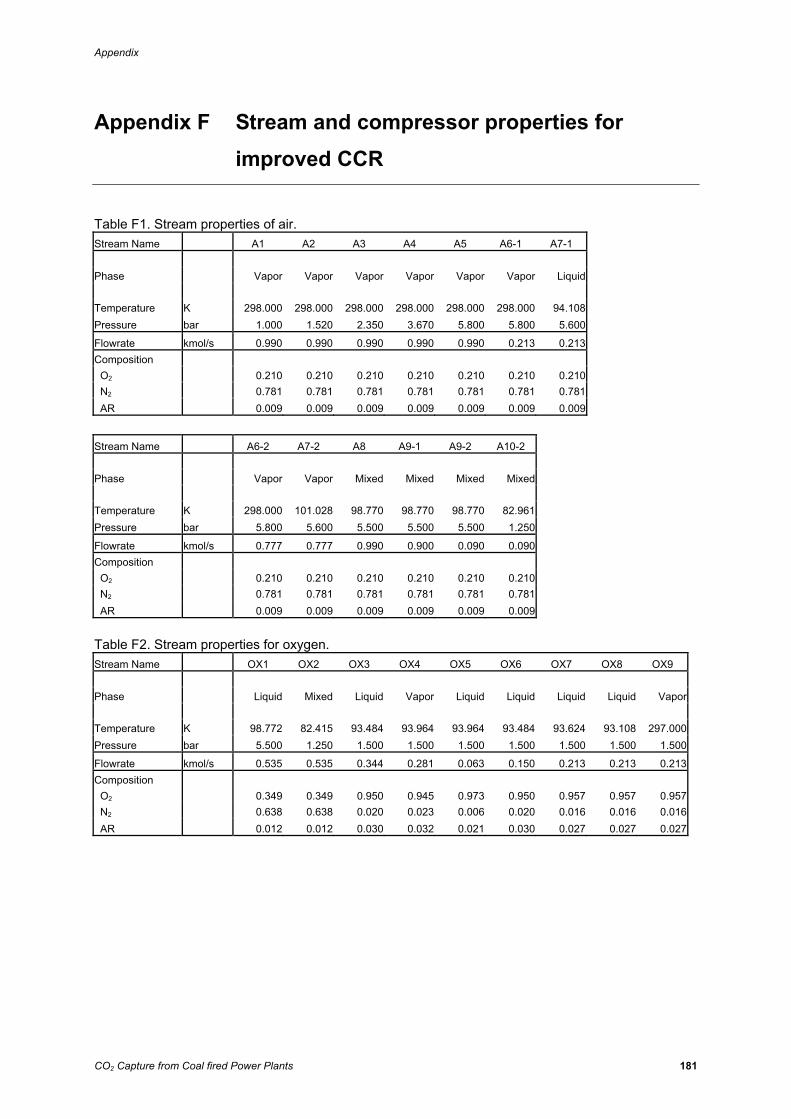
Appendix
CO2 Capture from Coal fired Power Plants 181
Appendix F Stream and compressor properties for improved CCR
Table F1. Stream properties of air. Stream Name A1 A2 A3 A4 A5 A6-1 A7-1 Phase Vapor Vapor Vapor Vapor Vapor Vapor Liquid Temperature K 298.000 298.000 298.000 298.000 298.000 298.000 94.108 Pressure bar 1.000 1.520 2.350 3.670 5.800 5.800 5.600
Flowrate kmol/s 0.990 0.990 0.990 0.990 0.990 0.213 0.213 Composition O2 0.210 0.210 0.210 0.210 0.210 0.210 0.210 N2 0.781 0.781 0.781 0.781 0.781 0.781 0.781 AR 0.009 0.009 0.009 0.009 0.009 0.009 0.009
Stream Name A6-2 A7-2 A8 A9-1 A9-2 A10-2 Phase Vapor Vapor Mixed Mixed Mixed Mixed Temperature K 298.000 101.028 98.770 98.770 98.770 82.961Pressure bar 5.800 5.600 5.500 5.500 5.500 1.250
Flowrate kmol/s 0.777 0.777 0.990 0.900 0.090 0.090Composition O2 0.210 0.210 0.210 0.210 0.210 0.210 N2 0.781 0.781 0.781 0.781 0.781 0.781 AR 0.009 0.009 0.009 0.009 0.009 0.009
Table F2. Stream properties for oxygen. Stream Name OX1 OX2 OX3 OX4 OX5 OX6 OX7 OX8 OX9 Phase Liquid Mixed Liquid Vapor Liquid Liquid Liquid Liquid Vapor Temperature K 98.772 82.415 93.484 93.964 93.964 93.484 93.624 93.108 297.000Pressure bar 5.500 1.250 1.500 1.500 1.500 1.500 1.500 1.500 1.500
Flowrate kmol/s 0.535 0.535 0.344 0.281 0.063 0.150 0.213 0.213 0.213Composition O2 0.349 0.349 0.950 0.945 0.973 0.950 0.957 0.957 0.957 N2 0.638 0.638 0.020 0.023 0.006 0.020 0.016 0.016 0.016 AR 0.012 0.012 0.030 0.032 0.021 0.030 0.027 0.027 0.027
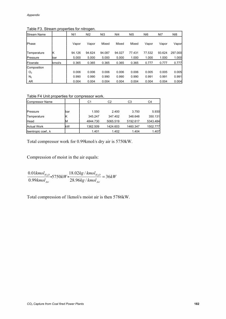
Appendix
CO2 Capture from Coal fired Power Plants 182
Table F3. Stream properties for nitrogen. Stream Name NI1 NI2 NI3 NI4 NI5 NI6 NI7 NI8 Phase Vapor Vapor Mixed Mixed Mixed Vapor Vapor Vapor Temperature K 94.126 94.624 94.087 94.027 77.431 77.532 93.624 297.000 Pressure bar 5.000 5.000 5.000 5.000 1.000 1.000 1.000 1.000
Flowrate kmol/s 0.365 0.365 0.365 0.365 0.365 0.777 0.777 0.777 Composition O2 0.006 0.006 0.006 0.006 0.006 0.005 0.005 0.005 N2 0.990 0.990 0.990 0.990 0.990 0.991 0.991 0.991 AR 0.004 0.004 0.004 0.004 0.004 0.004 0.004 0.004
Table F4 Unit properties for compressor work. Compressor Name C1 C2 C3 C4 Pressure bar 1.550 2.400 3.750 5.930Temperature K 345.247 347.402 348.648 350.131Head M 4844.730 5065.519 5192.617 5343.484
Actual Work kW 1362.509 1424.603 1460.347 1502.777Isentropic coef., k 1.401 1.402 1.404 1.407
Total compressor work for 0.99kmol/s dry air is 5750kW.
Compression of moist in the air equals:
2 20.01 18.02 /
5750 360.99 28.96 /
H O H O
Air Air
kmol kg kmolkW kW
kmol kg kmol=i i
Total compression of 1kmol/s moist air is then 5786kW.
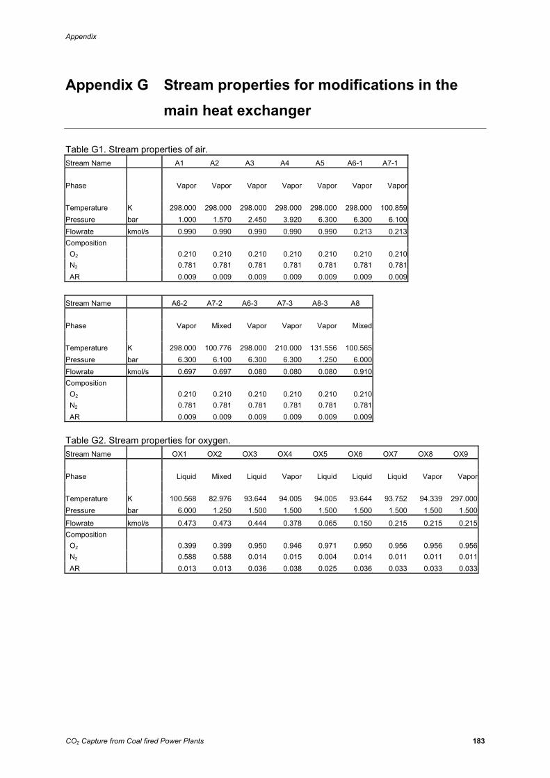
Appendix
CO2 Capture from Coal fired Power Plants 183
Appendix G Stream properties for modifications in the main heat exchanger
Table G1. Stream properties of air. Stream Name A1 A2 A3 A4 A5 A6-1 A7-1 Phase Vapor Vapor Vapor Vapor Vapor Vapor Vapor Temperature K 298.000 298.000 298.000 298.000 298.000 298.000 100.859 Pressure bar 1.000 1.570 2.450 3.920 6.300 6.300 6.100 Flowrate kmol/s 0.990 0.990 0.990 0.990 0.990 0.213 0.213 Composition O2 0.210 0.210 0.210 0.210 0.210 0.210 0.210 N2 0.781 0.781 0.781 0.781 0.781 0.781 0.781 AR 0.009 0.009 0.009 0.009 0.009 0.009 0.009
Stream Name A6-2 A7-2 A6-3 A7-3 A8-3 A8 Phase Vapor Mixed Vapor Vapor Vapor Mixed Temperature K 298.000 100.776 298.000 210.000 131.556 100.565Pressure bar 6.300 6.100 6.300 6.300 1.250 6.000Flowrate kmol/s 0.697 0.697 0.080 0.080 0.080 0.910Composition O2 0.210 0.210 0.210 0.210 0.210 0.210 N2 0.781 0.781 0.781 0.781 0.781 0.781 AR 0.009 0.009 0.009 0.009 0.009 0.009
Table G2. Stream properties for oxygen. Stream Name OX1 OX2 OX3 OX4 OX5 OX6 OX7 OX8 OX9 Phase Liquid Mixed Liquid Vapor Liquid Liquid Liquid Vapor Vapor Temperature K 100.568 82.976 93.644 94.005 94.005 93.644 93.752 94.339 297.000Pressure bar 6.000 1.250 1.500 1.500 1.500 1.500 1.500 1.500 1.500
Flowrate kmol/s 0.473 0.473 0.444 0.378 0.065 0.150 0.215 0.215 0.215Composition O2 0.399 0.399 0.950 0.946 0.971 0.950 0.956 0.956 0.956 N2 0.588 0.588 0.014 0.015 0.004 0.014 0.011 0.011 0.011 AR 0.013 0.013 0.036 0.038 0.025 0.036 0.033 0.033 0.033
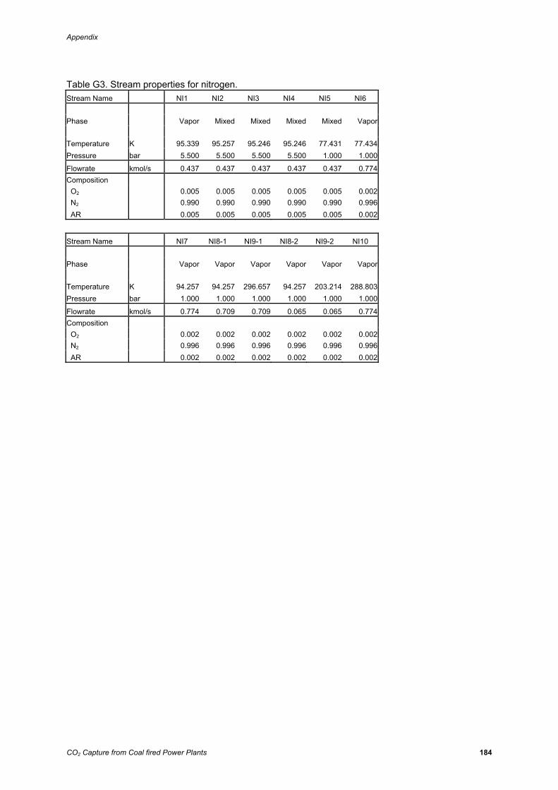
Appendix
CO2 Capture from Coal fired Power Plants 184
Table G3. Stream properties for nitrogen. Stream Name NI1 NI2 NI3 NI4 NI5 NI6 Phase Vapor Mixed Mixed Mixed Mixed Vapor Temperature K 95.339 95.257 95.246 95.246 77.431 77.434Pressure bar 5.500 5.500 5.500 5.500 1.000 1.000
Flowrate kmol/s 0.437 0.437 0.437 0.437 0.437 0.774Composition O2 0.005 0.005 0.005 0.005 0.005 0.002 N2 0.990 0.990 0.990 0.990 0.990 0.996 AR 0.005 0.005 0.005 0.005 0.005 0.002
Stream Name NI7 NI8-1 NI9-1 NI8-2 NI9-2 NI10 Phase Vapor Vapor Vapor Vapor Vapor Vapor Temperature K 94.257 94.257 296.657 94.257 203.214 288.803Pressure bar 1.000 1.000 1.000 1.000 1.000 1.000
Flowrate kmol/s 0.774 0.709 0.709 0.065 0.065 0.774Composition O2 0.002 0.002 0.002 0.002 0.002 0.002 N2 0.996 0.996 0.996 0.996 0.996 0.996 AR 0.002 0.002 0.002 0.002 0.002 0.002

Appendix
CO2 Capture from Coal fired Power Plants 185
Appendix H Number of compressors in ASU model
Total work to compress 1 kmol/s of dry air for different number of compressors. Table H1. One compressor. Compressor Name C1 Total work
Pressure bar 6.430 Temperature K 552.722
Head M 26479.143
Actual Work kW 7522.091 7522.091
Isentropic coef.. k 1.398
Table H2. Two compressors. Compressor Name C1 C2 Total work
Pressure bar 2.500 6.430 Temperature K 405.062 411.718
Head M 11009.189 11699.027
Actual Work kW 3127.447 3323.414 6450.861
Isentropic coef.. k 1.401 1.404
Table H3. Three compressors. Compressor Name C1 C2 C3 Total work
Pressure bar 1.800 3.300 6.430 Temperature K 362.975 367.981 375.469
Head M 6667.510 7181.967 7952.191
Actual Work kW 1894.080 2040.225 2259.028 6193.333
Isentropic coef.. k 1.401 1.403 1.406
Table H4. Four compressors. Compressor Name C1 C2 C3 C4 Total work
Pressure bar 1.500 2.300 3.800 6.430 Temperature K 341.472 346.342 355.338 358.132
Head M 4457.062 4956.693 5880.362 6166.210
Actual Work kW 1266.145 1408.078 1670.470 1751.673 6096.366
Isentropic coef.. k 1.401 1.402 1.404 1.407
Table H5. Five compressors. Compressor Name C1 C2 C3 C4 C5 Total work
Pressure bar 1.400 2.000 2.900 4.200 6.430 Temperature K 333.661 338.384 339.919 339.874 345.545
Head M 3655.170 4139.551 4296.444 4290.852 4871.360
Actual Work kW 1038.346 1175.948 1220.517 1218.929 1383.837 6037.576
Isentropic coef.. k 1.401 1.402 1.403 1.405 1.407
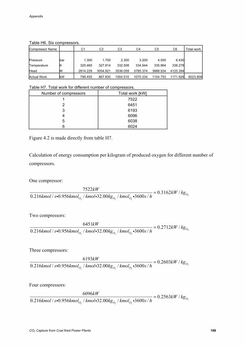
Appendix
CO2 Capture from Coal fired Power Plants 186
Table H6. Six compressors. Compressor Name C1 C2 C3 C4 C5 C6 Total work
Pressure bar 1.300 1.700 2.300 3.200 4.500 6.430 Temperature K 325.465 327.814 332.508 334.944 335.964 338.278
Head M 2814.229 3054.921 3536.059 3785.374 3888.934 4125.394
Actual Work kW 799.455 867.830 1004.510 1075.334 1104.753 1171.926 6023.808
Table H7. Total work for different number of compressors.
Number of compressors Total work [kW] 1 7522 2 6451 3 6193 4 6096 5 6038 6 6024
Figure 4.2 is made directly from table H7.
Calculation of energy consumption per kilogram of produced oxygen for different number of
compressors.
One compressor:
2
2 2 2
7522 0.3162 /0.216 / 0.956 / 32.00 / 3600 / O
O O O
kW kW kgkmol s kmol kmol kg kmol s h
=i i i
Two compressors:
2
2 2 2
6451 0.2712 /0.216 / 0.956 / 32.00 / 3600 / O
O O O
kW kW kgkmol s kmol kmol kg kmol s h
=i i i
Three compressors:
2
2 2 2
6193 0.2603 /0.216 / 0.956 / 32.00 / 3600 / O
O O O
kW kW kgkmol s kmol kmol kg kmol s h
=i i i
Four compressors:
2
2 2 2
6096 0.2563 /0.216 / 0.956 / 32.00 / 3600 / O
O O O
kW kW kgkmol s kmol kmol kg kmol s h
=i i i
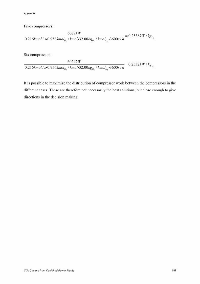
Appendix
CO2 Capture from Coal fired Power Plants 187
Five compressors:
2
2 2 2
6038 0.2538 /0.216 / 0.956 / 32.00 / 3600 / O
O O O
kW kW kgkmol s kmol kmol kg kmol s h
=i i i
Six compressors:
2
2 2 2
6024 0.2532 /0.216 / 0.956 / 32.00 / 3600 / O
O O O
kW kW kgkmol s kmol kmol kg kmol s h
=i i i
It is possible to maximize the distribution of compressor work between the compressors in the
different cases. These are therefore not necessarily the best solutions, but close enough to give
directions in the decision making.
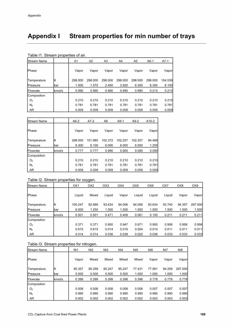
Appendix
CO2 Capture from Coal fired Power Plants 188
Appendix I Stream properties for min number of trays
Table I1. Stream properties of air. Stream Name A1 A2 A3 A4 A5 A6-1 A7-1 Phase Vapor Vapor Vapor Vapor Vapor Vapor Vapor Temperature K 298.000 298.000 298.000 298.000 298.000 298.000 104.539 Pressure bar 1.000 1.570 2.450 3.920 6.300 6.300 6.100
Flowrate kmol/s 0.990 0.990 0.990 0.990 0.990 0.213 0.213 Composition O2 0.210 0.210 0.210 0.210 0.210 0.210 0.210 N2 0.781 0.781 0.781 0.781 0.781 0.781 0.781 AR 0.009 0.009 0.009 0.009 0.009 0.009 0.009
Stream Name A6-2 A7-2 A8 A9-1 A9-2 A10-2 Phase Vapor Vapor Vapor Vapor Vapor Vapor Temperature K 298.000 101.985 102.372 102.257 102.257 94.466Pressure bar 6.300 6.100 6.000 6.000 6.000 1.250
Flowrate kmol/s 0.777 0.777 0.990 0.900 0.090 0.090Composition O2 0.210 0.210 0.210 0.210 0.210 0.210 N2 0.781 0.781 0.781 0.781 0.781 0.781 AR 0.009 0.009 0.009 0.009 0.009 0.009
Table I2. Stream properties for oxygen. Stream Name OX1 OX2 OX3 OX4 OX5 OX6 OX7 OX8 OX9 Phase Liquid Mixed Liquid Vapor Liquid Liquid Liquid Vapor Vapor Temperature K 100.247 82.689 93.634 94.006 94.006 93.634 93.740 94.357 297.000Pressure bar 6.000 1.250 1.500 1.500 1.500 1.500 1.500 1.500 1.500
Flowrate kmol/s 0.501 0.501 0.471 0.409 0.061 0.150 0.211 0.211 0.211Composition O2 0.371 0.371 0.950 0.947 0.971 0.950 0.956 0.956 0.956 N2 0.615 0.615 0.014 0.016 0.004 0.014 0.011 0.011 0.011 AR 0.014 0.014 0.036 0.038 0.025 0.036 0.033 0.033 0.033
Table I3. Stream properties for nitrogen. Stream Name NI1 NI2 NI3 NI4 NI5 NI6 NI7 NI8 Phase Vapor Mixed Mixed Mixed Mixed Vapor Vapor Vapor Temperature K 95.357 95.259 95.247 95.247 77.431 77.561 94.259 297.000 Pressure bar 5.500 5.500 5.500 5.500 1.000 1.000 1.000 1.000
Flowrate kmol/s 0.399 0.399 0.399 0.398 0.398 0.778 0.778 0.778 Composition O2 0.008 0.008 0.008 0.008 0.008 0.007 0.007 0.007 N2 0.990 0.990 0.990 0.990 0.990 0.990 0.990 0.990 AR 0.002 0.002 0.002 0.002 0.002 0.003 0.003 0.003
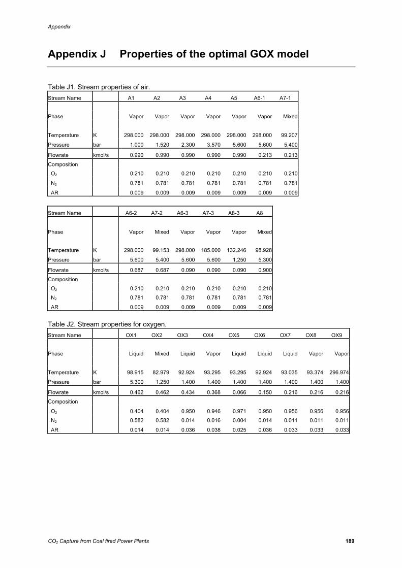
Appendix
CO2 Capture from Coal fired Power Plants 189
Appendix J Properties of the optimal GOX model
Table J1. Stream properties of air. Stream Name A1 A2 A3 A4 A5 A6-1 A7-1
Phase Vapor Vapor Vapor Vapor Vapor Vapor Mixed
Temperature K 298.000 298.000 298.000 298.000 298.000 298.000 99.207
Pressure bar 1.000 1.520 2.300 3.570 5.600 5.600 5.400
Flowrate kmol/s 0.990 0.990 0.990 0.990 0.990 0.213 0.213
Composition
O2 0.210 0.210 0.210 0.210 0.210 0.210 0.210
N2 0.781 0.781 0.781 0.781 0.781 0.781 0.781
AR 0.009 0.009 0.009 0.009 0.009 0.009 0.009
Stream Name A6-2 A7-2 A6-3 A7-3 A8-3 A8
Phase Vapor Mixed Vapor Vapor Vapor Mixed
Temperature K 298.000 99.153 298.000 185.000 132.246 98.928
Pressure bar 5.600 5.400 5.600 5.600 1.250 5.300
Flowrate kmol/s 0.687 0.687 0.090 0.090 0.090 0.900
Composition
O2 0.210 0.210 0.210 0.210 0.210 0.210
N2 0.781 0.781 0.781 0.781 0.781 0.781
AR 0.009 0.009 0.009 0.009 0.009 0.009
Table J2. Stream properties for oxygen. Stream Name OX1 OX2 OX3 OX4 OX5 OX6 OX7 OX8 OX9
Phase Liquid Mixed Liquid Vapor Liquid Liquid Liquid Vapor Vapor
Temperature K 98.915 82.979 92.924 93.295 93.295 92.924 93.035 93.374 296.974
Pressure bar 5.300 1.250 1.400 1.400 1.400 1.400 1.400 1.400 1.400
Flowrate kmol/s 0.462 0.462 0.434 0.368 0.066 0.150 0.216 0.216 0.216
Composition
O2 0.404 0.404 0.950 0.946 0.971 0.950 0.956 0.956 0.956
N2 0.582 0.582 0.014 0.016 0.004 0.014 0.011 0.011 0.011
AR 0.014 0.014 0.036 0.038 0.025 0.036 0.033 0.033 0.033
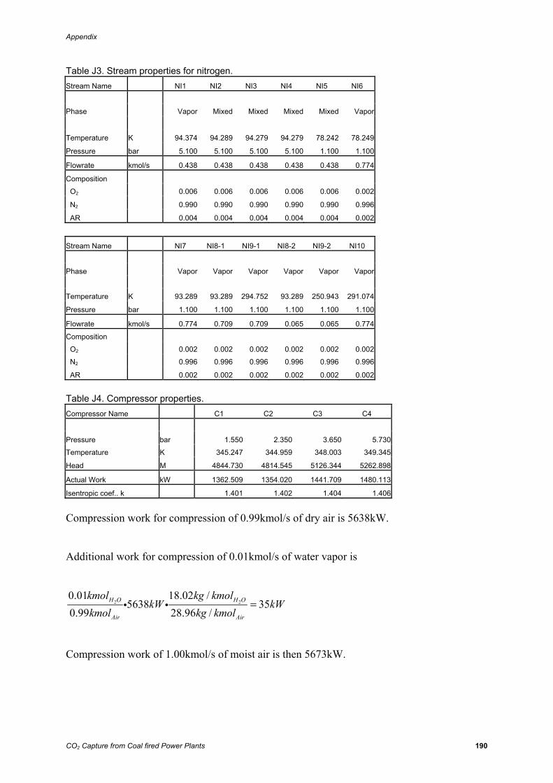
Appendix
CO2 Capture from Coal fired Power Plants 190
Table J3. Stream properties for nitrogen. Stream Name NI1 NI2 NI3 NI4 NI5 NI6
Phase Vapor Mixed Mixed Mixed Mixed Vapor
Temperature K 94.374 94.289 94.279 94.279 78.242 78.249
Pressure bar 5.100 5.100 5.100 5.100 1.100 1.100
Flowrate kmol/s 0.438 0.438 0.438 0.438 0.438 0.774
Composition
O2 0.006 0.006 0.006 0.006 0.006 0.002
N2 0.990 0.990 0.990 0.990 0.990 0.996
AR 0.004 0.004 0.004 0.004 0.004 0.002
Stream Name NI7 NI8-1 NI9-1 NI8-2 NI9-2 NI10
Phase Vapor Vapor Vapor Vapor Vapor Vapor
Temperature K 93.289 93.289 294.752 93.289 250.943 291.074
Pressure bar 1.100 1.100 1.100 1.100 1.100 1.100
Flowrate kmol/s 0.774 0.709 0.709 0.065 0.065 0.774
Composition
O2 0.002 0.002 0.002 0.002 0.002 0.002
N2 0.996 0.996 0.996 0.996 0.996 0.996
AR 0.002 0.002 0.002 0.002 0.002 0.002
Table J4. Compressor properties. Compressor Name C1 C2 C3 C4
Pressure bar 1.550 2.350 3.650 5.730
Temperature K 345.247 344.959 348.003 349.345
Head M 4844.730 4814.545 5126.344 5262.898
Actual Work kW 1362.509 1354.020 1441.709 1480.113
Isentropic coef.. k 1.401 1.402 1.404 1.406
Compression work for compression of 0.99kmol/s of dry air is 5638kW.
Additional work for compression of 0.01kmol/s of water vapor is
2 20.01 18.02 /
5638 350.99 28.96 /
H O H O
Air Air
kmol kg kmolkW kW
kmol kg kmol=i i
Compression work of 1.00kmol/s of moist air is then 5673kW.

Appendix
CO2 Capture from Coal fired Power Plants 191
Table J5. Heat exchanger properties. Hx Name E1 E2 E3 E4 E5 E6
Main heat ex Main heat ex Subcooler Subcooler Convergence Comb cond-reb
Duty MW 1.2812 4.1899 1.4702 0.3507 0.0007 2.5098
Table J6. Column properties. Column Name HP LP
Condenser Duty MW -2.5098 n/a
Reboiler Duty MW n/a -0.0003
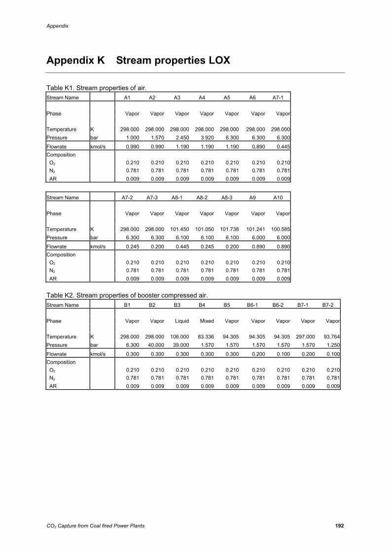
Appendix
CO2 Capture from Coal fired Power Plants 192
Appendix K Stream properties LOX
Table K1. Stream properties of air. Stream Name A1 A2 A3 A4 A5 A6 A7-1 Phase Vapor Vapor Vapor Vapor Vapor Vapor Vapor Temperature K 298.000 298.000 298.000 298.000 298.000 298.000 298.000 Pressure bar 1.000 1.570 2.450 3.920 6.300 6.300 6.300
Flowrate kmol/s 0.990 0.990 1.190 1.190 1.190 0.890 0.445 Composition O2 0.210 0.210 0.210 0.210 0.210 0.210 0.210 N2 0.781 0.781 0.781 0.781 0.781 0.781 0.781 AR 0.009 0.009 0.009 0.009 0.009 0.009 0.009
Stream Name A7-2 A7-3 A8-1 A8-2 A8-3 A9 A10 Phase Vapor Vapor Vapor Vapor Vapor Vapor Vapor Temperature K 298.000 298.000 101.450 101.050 101.738 101.241 100.585 Pressure bar 6.300 6.300 6.100 6.100 6.100 6.000 6.000
Flowrate kmol/s 0.245 0.200 0.445 0.245 0.200 0.890 0.890 Composition O2 0.210 0.210 0.210 0.210 0.210 0.210 0.210 N2 0.781 0.781 0.781 0.781 0.781 0.781 0.781 AR 0.009 0.009 0.009 0.009 0.009 0.009 0.009
Table K2. Stream properties of booster compressed air. Stream Name B1 B2 B3 B4 B5 B6-1 B6-2 B7-1 B7-2 Phase Vapor Vapor Liquid Mixed Vapor Vapor Vapor Vapor Vapor Temperature K 298.000 298.000 106.000 83.336 94.305 94.305 94.305 297.000 93.764Pressure bar 6.300 40.000 39.000 1.570 1.570 1.570 1.570 1.570 1.250
Flowrate kmol/s 0.300 0.300 0.300 0.300 0.300 0.200 0.100 0.200 0.100Composition O2 0.210 0.210 0.210 0.210 0.210 0.210 0.210 0.210 0.210 N2 0.781 0.781 0.781 0.781 0.781 0.781 0.781 0.781 0.781 AR 0.009 0.009 0.009 0.009 0.009 0.009 0.009 0.009 0.009
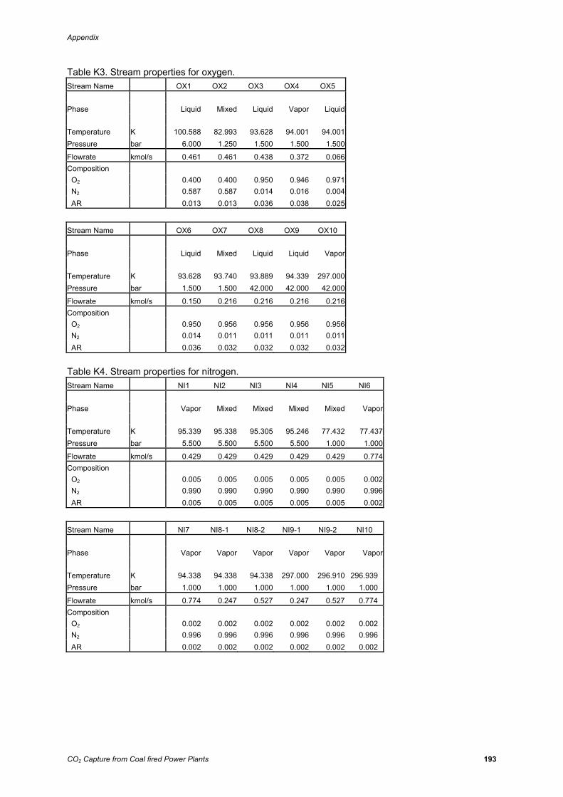
Appendix
CO2 Capture from Coal fired Power Plants 193
Table K3. Stream properties for oxygen. Stream Name OX1 OX2 OX3 OX4 OX5 Phase Liquid Mixed Liquid Vapor Liquid Temperature K 100.588 82.993 93.628 94.001 94.001Pressure bar 6.000 1.250 1.500 1.500 1.500
Flowrate kmol/s 0.461 0.461 0.438 0.372 0.066Composition O2 0.400 0.400 0.950 0.946 0.971 N2 0.587 0.587 0.014 0.016 0.004 AR 0.013 0.013 0.036 0.038 0.025
Stream Name OX6 OX7 OX8 OX9 OX10 Phase Liquid Mixed Liquid Liquid Vapor Temperature K 93.628 93.740 93.889 94.339 297.000Pressure bar 1.500 1.500 42.000 42.000 42.000
Flowrate kmol/s 0.150 0.216 0.216 0.216 0.216Composition O2 0.950 0.956 0.956 0.956 0.956 N2 0.014 0.011 0.011 0.011 0.011 AR 0.036 0.032 0.032 0.032 0.032
Table K4. Stream properties for nitrogen. Stream Name NI1 NI2 NI3 NI4 NI5 NI6 Phase Vapor Mixed Mixed Mixed Mixed Vapor Temperature K 95.339 95.338 95.305 95.246 77.432 77.437Pressure bar 5.500 5.500 5.500 5.500 1.000 1.000
Flowrate kmol/s 0.429 0.429 0.429 0.429 0.429 0.774Composition O2 0.005 0.005 0.005 0.005 0.005 0.002 N2 0.990 0.990 0.990 0.990 0.990 0.996 AR 0.005 0.005 0.005 0.005 0.005 0.002
Stream Name NI7 NI8-1 NI8-2 NI9-1 NI9-2 NI10 Phase Vapor Vapor Vapor Vapor Vapor Vapor Temperature K 94.338 94.338 94.338 297.000 296.910 296.939 Pressure bar 1.000 1.000 1.000 1.000 1.000 1.000
Flowrate kmol/s 0.774 0.247 0.527 0.247 0.527 0.774 Composition O2 0.002 0.002 0.002 0.002 0.002 0.002 N2 0.996 0.996 0.996 0.996 0.996 0.996 AR 0.002 0.002 0.002 0.002 0.002 0.002
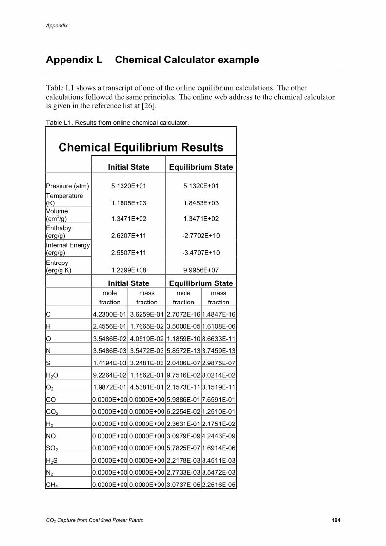
Appendix
CO2 Capture from Coal fired Power Plants 194
Appendix L Chemical Calculator example
Table L1 shows a transcript of one of the online equilibrium calculations. The other calculations followed the same principles. The online web address to the chemical calculator is given in the reference list at [26]. Table L1. Results from online chemical calculator.
Chemical Equilibrium Results Initial State Equilibrium State
Pressure (atm) 5.1320E+01 5.1320E+01 Temperature (K) 1.1805E+03 1.8453E+03 Volume (cm3/g) 1.3471E+02 1.3471E+02 Enthalpy (erg/g) 2.6207E+11 -2.7702E+10 Internal Energy (erg/g) 2.5507E+11 -3.4707E+10 Entropy (erg/g K) 1.2299E+08 9.9956E+07
Initial State Equilibrium Statemole mass mole mass
fraction fraction fraction fraction
C 4.2300E-01 3.6259E-01 2.7072E-16 1.4847E-16
H 2.4556E-01 1.7665E-02 3.5000E-05 1.6108E-06
O 3.5486E-02 4.0519E-02 1.1859E-10 8.6633E-11
N 3.5486E-03 3.5472E-03 5.8572E-13 3.7459E-13
S 1.4194E-03 3.2481E-03 2.0406E-07 2.9875E-07
H2O 9.2264E-02 1.1862E-01 9.7516E-02 8.0214E-02
O2 1.9872E-01 4.5381E-01 2.1573E-11 3.1519E-11
CO 0.0000E+00 0.0000E+00 5.9886E-01 7.6591E-01
CO2 0.0000E+00 0.0000E+00 6.2254E-02 1.2510E-01
H2 0.0000E+00 0.0000E+00 2.3631E-01 2.1751E-02
NO 0.0000E+00 0.0000E+00 3.0979E-09 4.2443E-09
SO2 0.0000E+00 0.0000E+00 5.7825E-07 1.6914E-06
H2S 0.0000E+00 0.0000E+00 2.2178E-03 3.4511E-03
N2 0.0000E+00 0.0000E+00 2.7733E-03 3.5472E-03
CH4 0.0000E+00 0.0000E+00 3.0737E-05 2.2516E-05
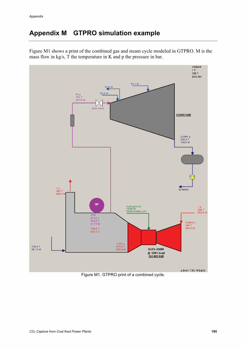
Appendix
CO2 Capture from Coal fired Power Plants 195
Appendix M GTPRO simulation example
Figure M1 shows a print of the combined gas and steam cycle modeled in GTPRO. M is the mass flow in kg/s, T the temperature in K and p the pressure in bar.
Figure M1. GTPRO print of a combined cycle.
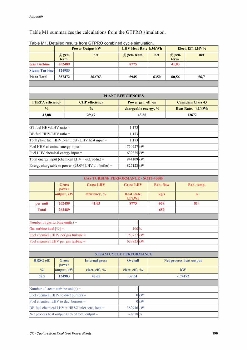
Appendix
CO2 Capture from Coal fired Power Plants 196
Table M1 summarizes the calculations from the GTPRO simulation. Table M1. Detailed results from GTPRO combined cycle simulation.
Power Output kW LHV Heat Rate kJ/kWh Elect. Eff. LHV%
@ gen. term.
net @ gen. term. net @ gen. term.
net
Gas Turbine 262489 8775 41,03
Steam Turbine 124983
Plant Total 387472 362763 5945 6350 60,56 56,7
PLANT EFFICIENCIES
PURPA efficiency CHP efficiency Power gen. eff. on Canadian Class 43
% % chargeable energy, % Heat Rate, kJ/kWh
43,08 29,47 43,86 12672
GT fuel HHV/LHV ratio = 1,173
DB fuel HHV/LHV ratio = 1,173
Total plant fuel HHV heat input / LHV heat input = 1,173
Fuel HHV chemical energy input = 750727 kW
Fuel LHV chemical energy input = 639825 kW
Total energy input (chemical LHV + ext. addn.) = 944109 kW
Energy chargeable to power (93,0% LHV alt. boiler) = 827128 kW
GAS TURBINE PERFORMANCE - SGT5-4000F
Gross power
Gross LHV Gross LHV Exh. flow Exh. temp.
output, kW efficiency, % Heat Rate, kJ/kWh
kg/s K
per unit 262489 41,03 8775 659 814
Total 262489 659
Number of gas turbine unit(s) = 1
Gas turbine load [%] = 100 %
Fuel chemical HHV per gas turbine = 750727 kW
Fuel chemical LHV per gas turbine = 639825 kW
STEAM CYCLE PERFORMANCE
HRSG eff. Gross power
Internal gross Overall Net process heat output
% output, kW elect. eff., % elect. eff., % kW
68,5 124983 47,65 32,64 -174192
Number of steam turbine unit(s) = 1
Fuel chemical HHV to duct burners = 0 kW
Fuel chemical LHV to duct burners = 0 kW
DB fuel chemical LHV + HRSG inlet sens. heat = 382946 kW
Net process heat output as % of total output = -92,38 %
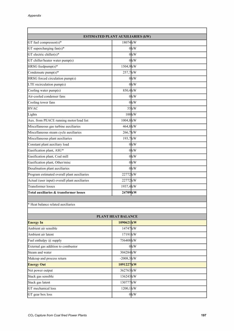
Appendix
CO2 Capture from Coal fired Power Plants 197
ESTIMATED PLANT AUXILIARIES (kW)
GT fuel compressor(s)* 18074 kW
GT supercharging fan(s)* 0 kW
GT electric chiller(s)* 0 kW
GT chiller/heater water pump(s) 0 kW
HRSG feedpump(s)* 1504,9 kW
Condensate pump(s)* 257,7 kW
HRSG forced circulation pump(s) 0 kW
LTE recirculation pump(s) 0 kW
Cooling water pump(s) 850,4 kW
Air-cooled condenser fans 0 kW
Cooling tower fans 0 kW
HVAC 55 kW
Lights 100 kW
Aux. from PEACE running motor/load list 1004,8 kW
Miscellaneous gas turbine auxiliaries 464,8 kW
Miscellaneous steam cycle auxiliaries 266,7 kW
Miscellaneous plant auxiliaries 193,7 kW
Constant plant auxiliary load 0 kW
Gasification plant, ASU* 0 kW
Gasification plant, Coal mill 0 kW
Gasification plant, Other/misc 0 kW
Desalination plant auxiliaries 0 kW
Program estimated overall plant auxiliaries 22772 kW
Actual (user input) overall plant auxiliaries 22772 kW
Transformer losses 1937,4 kW
Total auxiliaries & transformer losses 24709 kW
* Heat balance related auxiliaries
PLANT HEAT BALANCE
Energy In 1090621 kW
Ambient air sensible 14747 kW
Ambient air latent 17191 kW
Fuel enthalpy @ supply 756408 kW
External gas addition to combustor 0 kW
Steam and water 304284 kW
Makeup and process return -2008,3 kW
Energy Out 1091227 kW
Net power output 362763 kW
Stack gas sensible 136243 kW
Stack gas latent 130777 kW
GT mechanical loss 1200,1 kW
GT gear box loss 0 kW
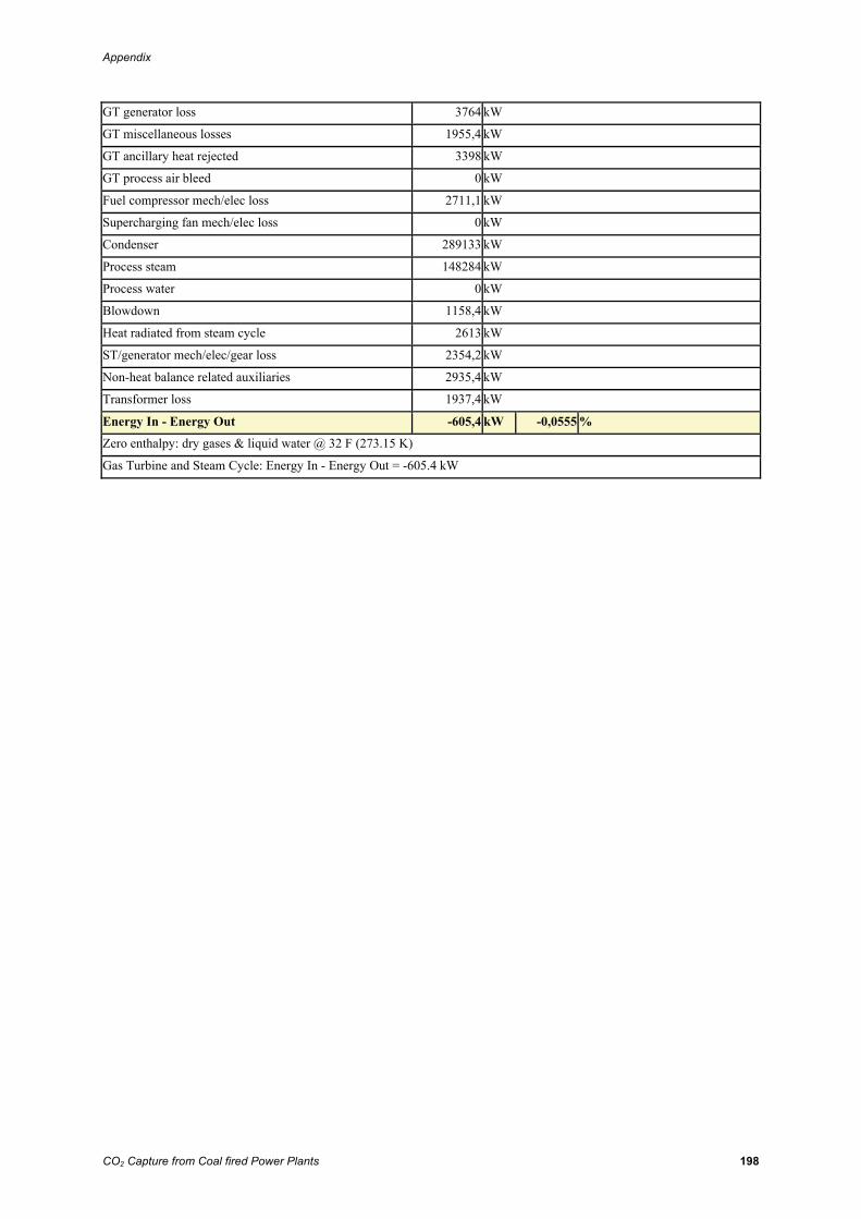
Appendix
CO2 Capture from Coal fired Power Plants 198
GT generator loss 3764 kW
GT miscellaneous losses 1955,4 kW
GT ancillary heat rejected 3398 kW
GT process air bleed 0 kW
Fuel compressor mech/elec loss 2711,1 kW
Supercharging fan mech/elec loss 0 kW
Condenser 289133 kW
Process steam 148284 kW
Process water 0 kW
Blowdown 1158,4 kW
Heat radiated from steam cycle 2613 kW
ST/generator mech/elec/gear loss 2354,2 kW
Non-heat balance related auxiliaries 2935,4 kW
Transformer loss 1937,4 kW
Energy In - Energy Out -605,4 kW -0,0555 %
Zero enthalpy: dry gases & liquid water @ 32 F (273.15 K)
Gas Turbine and Steam Cycle: Energy In - Energy Out = -605.4 kW