1

Paper for ECB Sintra Forum 2021

Climate Policies and Monetary Policies

in the Euro Area1

Warwick McKibbin2, Maximilian Konradt3 and Beatrice Weder di Mauro4

Forum Draft

This paper presents two types of analysis on the interaction between policies to deal with climate change and monetary policies in the euro area. First, we empirically analyze the historical effects of carbon taxes on inflation in the euro area countries to gauge the impact under the current European monetary regime. Second, we explore two alternative monetary policy rules under a range of simulations in a new European version of the G-Cubed multisector model. We study the economic and inflationary impacts of physical climate change shocks (climate risk) and transitions risks arising from carbon taxation within Europe and globally. We find that under the existing monetary policy framework, the inflationary effects of carbon taxes in Euro area countries have been contained. The only significant increase in the HICP (of about 0.8 index points) is found in the first two years. At the same time, however, the impact on core inflation tended to be negative. Thus, carbon taxes mainly affected relative prices rather than the overall price level, which is in line with previous findings for a broader sample of countries. We also find that producers seem to have absorbed a part of the carbon tax since consumer price inflation was lower than producer price inflation.

The results from the simulation model show that the nature of the monetary rule within Europe has a significant effect on the impact of climate shocks and climate policy changes within Europe. An entirely forward-looking rule proposed by Hartmann and Smets (2018) may lead to excessively tight monetary policy in the face of climate shocks and climate policy changes within Europe. An alternate modified version of this rule that puts equal weights on current and forward-looking variables leads to a better short-run outcome for Europe. We also find a difference in results for Europe between the impact of climate policy implemented only within the Euro area and climate policy implemented globally. The main difference is the impact of global policies versus Euro area policies on international capital flows and the exchange rate. Overall, the model simulations suggest that physical climate risk as well as transitions risks from carbon pricing have long run output costs but only a transitory impact on inflation. Moreover, the price reaction critically depends on the monetary policy regime, which may result either in inflation or deflation in the short run.

1 We thank Philipp Hartman, Frank Elderson and a discussant at the ECB for helpful comments and suggestions. McKibbin also acknowledges the contributions of Peter Wilcoxen and Larry Weifeng Liu to the development of on the G-Cubed model and thanks the Australian Research Council Centre of Excellence in Population Ageing Research for additional financial support (CE170100005). 2 ANU Crawford School of Public Policy, CEPAR, CEPR, The Brookings Institution 3 Graduate Institute, Geneva 4 Graduate Institute, Geneva, CEPR, INSEAD.

2

1. Introduction:

The 2021 strategy review of the ECB has surprised observers with the strength of their commitment to incorporate climate change in the monetary policy framework. The ECB board clearly states that the transition to a more sustainable economy will affect the outlook for inflation, output, employment, interest rates, investment, productivity, and financial stability, and the transmission of monetary policy.5 Consequently, the ECB announced an ambitious and detailed roadmap on climate-related actions.

One of the key elements of the action plan is strengthening the analytical foundations for gradually incorporating climate change risks in macroeconomic models and monetary policy frameworks. The ECB plans to start immediately to use assumptions on carbon pricing in its regular forecasting. Over the next three years, the ECB plans to integrate climate risks into its workhorse models to assess the impacts on potential growth and monetary policy transmission.6

The focus on the effects of climate change on inflation is novel. Most of the current climate-related macro literature has focused on economic growth costs of climate risks. Also, current worries about higher inflation rates have been associated with fears that CO2 pricing will accelerate price dynamics permanently.7

This paper aims to contribute to the ECBs’ macroeconomic action plan with two distinct but related analyses for the euro area. The first is an empirical study of the inflationary effects of carbon taxes in countries within the euro area over the past three decades. The second is model simulations using the G-Cubed model exploring the economic impact under different climate shocks, CO2 taxes, and monetary policy reaction functions.

It is worth briefly discussing differences between the scenarios in this paper with those from the Impact Assessment Models (IAM), which are currently used by the Network for Greening the Financial System (NGFS) to quantify climate risks.

A key difference is in the assumption on the level of carbon tax/price. In the G-Cubed model, we simulate a carbon tax of 50 Euros with a yearly increase of 3 percent, under two assumptions: 1) The tax is only implemented in Europe; 2) and the carbon tax is implemented globally. Whether this is a sufficiently high carbon price to achieve the Paris Agreement goal can be debated, some studies suggest that a carbon price implemented through a market mechanism can induce sufficient substitution in consumption and production to achieve the Paris targets by 20308. We use this price as

5 https://www.ecb.europa.eu/press/pr/date/2021/html/ecb.pr210708_1~f104919225.en.htm 6 https://www.ecb.europa.eu/press/pr/date/2021/html/ecb.pr210708_1_annex~f84ab35968.en.pdf 7 https://www.bis.org/review/r210702k.htm 8 See Liu, McKibbin Morris, and Wilcoxen (2020), using the G-Cubed model of this paper.

3

a baseline since it can be a realistic policy perspective/ambition for a global carbon price.

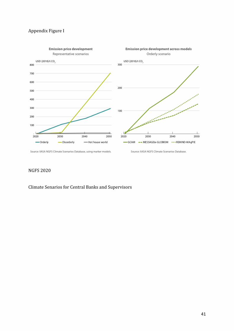
By contrast, emission prices underlying NGFS scenarios range up to $100 per ton by 2030 and from 300 to 700 USD/t CO2 by 2050(see Appendix Figure 1). These higher numbers are because the NGFS uses a different assumption for emission pricing to produce its climate scenarios: emission prices are estimated as the marginal abatement cost necessary to reach a specific temperature increase and thus depend on policy intensity and timing (NGFS 2020). These can be considered “shadow prices” for the costs of changing technology and capital in critical sectors. For instance, in a “hot house world,” governments do not fight climate change. The price of emissions is zero, and emissions continue to increase and at the globe warms up by more than 3 degrees. In a transition scenario, prices are calculated to be consistent with a pre-defined temperature target (e.g., 67% chance of limiting global warming to 2°C).

For example, the main NGFS orderly transition scenario has emission prices rising quickly to about 100 USD by 2030 and then steadily increasing to 300 USD by 2050. 9 By contrast, in the NGFS disorderly transition scenario, policy action is delayed, policymakers only wake up in 2030 and by then the necessary emission price path to limit warming to 2 degrees is much steeper and the end price rises to 700 USD.

Simulating a CO2 tax of up to 700 Euro in G-Cubed would not be practical for computational reasons. 10 More importantly, in practice, climate policies in Europe - and even more so in the US - will not load fully on carbon pricing to achieve the emission goals. Instead, they will rely on a combination of pricing and quantity restrictions, prohibitions, as well as subsidies and technological innovation. The European Green Deal, Fit for 55, explicitly endorses a philosophy for combining CO2 pricing which regulation and standards. An example is transport sector, where a end of the combustion engine for 2035 is combined with carbon pricing through ETS.

There are other differences in the model frameworks of the G-Cubed model and the IAMs11. A key difference is the detailed modeling of consumption and production decisions at sectoral levels across countries in the G-Cubed model compared to a simplified model of aggregate GDP in IAMs. There are also differences in the scenarios usually modeled. In addition, there is a difference between market-determined carbon prices or carbon taxes in the G-Cubed model and the shadow prices calculated from the

9 Different IAMs underlying the orderly transition scenario deliver a wide range of end prices, with the lowest at about 120 USD. 10 Such and extreme scenario could not be computed in G-Cubed. 11 The G-Cubed model and a range of other models in the climate change literature that are not IAMs regularly participate in the Stanford University, Energy Modeling Forum project coordinated by John Weyant. See Fawcett et al (2018). EMF is a useful source of model comparisons and policy analysis. https://emf.stanford.edu/projects/emf-32-us-ghg-and-revenue-recycling-scenarios

4

potentially inefficient regulatory policy in IAMs. It is not surprising that our simulations with the G-Cubed model are less extreme than the results of the IAM models.

While the NGFS scenarios illustrate the consequences of delayed policy action (and thus contribute to spur government intervention), our G-Cubed results focus on short- to medium-run macroeconomic dynamics under climate shocks and carbon taxes. This time frame may be more appropriate for the needs and time horizon of monetary policy. Thus, the two sets of analysis are complementary in that they are focused on different time frames and different types of policy interventions.

2. Carbon taxes and price dynamics: Evidence from the Euro Area

This section analyzes the historical impacts of carbon taxes implemented in countries within the Euro area between 1985 and 2020. We focus on the consequences for CPI inflation under the monetary regime in place when implementing the tax.

Data

For the empirical analysis, we use data on carbon taxes and economic aggregates. Our data on carbon tax rates and tax bases are from the Carbon Pricing Dashboard of the World Bank. We consider all Euro area countries with available data between 1985 and 2020. In that period, eight Euro area countries implemented carbon taxes at a national level, summarized in Table 1. All tax rates (columns 3-4) are expressed in real 2018 DM/EUR per ton of carbon dioxide equivalent emissions.

The 2020 tax rates might be affected by a countries' efforts to reduce the economic burden during Covid-19. For instance, the French tax dropped from a rate of 45 to 6€/tCO2e.12 The emission coverage (column 5) indicates the share of a country’s total greenhouse gas emissions covered by the carbon tax.

We are interested in the economic effect of carbon taxes. To that end, we look at a range of indicators as dependent variables in our estimations. Our sample consists of 17 Euro area member countries, excluding only Cyprus and Malta due to data limitations. The main variables used for the empirical analysis are summarized in Table 2.

Our data on GDP per capita are from the World Bank and expressed in real DM/EUR using the German GDP deflator. Data on the consumer price index (CPI) and producer price index (PPI) are retrieved from the OECD. We also explore core CPI (excluding energy and food) and the harmonized index of consumer prices (HICP) from Eurostat. All index variables are calculated with the base year 2018.

12 Some countries seem to be using CO2 pricing anti-cyclically. While this may increase the automatic fiscal stabilizers it counteracts the goal of emission reduction.

5

Table 1. Carbon taxes in the Euro area

Table 2. Descriptive Statistics on dependent variables

Estimation

To assess the effect of carbon taxation on the various economic variable, we estimate dynamic impulse responses using the local projections method (Jordà, 2005). Our estimations follow in the spirit of Metcalf and Stock (2020). Specifically, we estimate a sequence of OLS models (depicted here for CPI as a dependent variable):

𝛥𝛥𝐶𝐶𝐶𝐶𝐶𝐶 𝑖𝑖,𝑡𝑡+ℎ = 𝛼𝛼𝑖𝑖 + 𝛩𝛩ℎ𝜏𝜏𝑖𝑖,𝑡𝑡 + 𝛽𝛽(𝐿𝐿)𝜏𝜏𝑖𝑖,𝑡𝑡−1 + 𝛿𝛿(𝐿𝐿)𝛥𝛥𝐶𝐶𝐶𝐶𝐶𝐶𝑖𝑖,𝑡𝑡−1 + 𝛾𝛾𝑡𝑡 + 𝜖𝜖𝑖𝑖,𝑡𝑡

where 𝜏𝜏𝑖𝑖,𝑡𝑡 is the real carbon tax rate in country 𝑖𝑖 in year 𝑡𝑡. 𝛩𝛩ℎ is the effect of an unexpected change in the carbon tax at year 𝑡𝑡 on CPI, ℎ years ahead. To control for the

6

persistence of the tax rate and CPI, we include the four latest lags of each variable in the regression. A set of fixed effects, 𝛼𝛼𝑖𝑖 and 𝛾𝛾𝑡𝑡 absorbs unobserved heterogeneity specific to each country or year. 𝜖𝜖𝑖𝑖,𝑡𝑡 is an error term.

Dynamic impulse responses are estimated from annual data between 1985 and 2020 for each dependent variable, respectively. The sample is restricted to all Euro area countries with available data. Following Metcalf and Stock (2020), we weight all carbon taxes with their 2019 emission share, postulating that the economic effect of a carbon tax is proportional to its coverage. Standard errors are heteroscedasticity-robust (Plagborg-Møller and Wolf 2021).

Our counterfactual scenario considers a flat €40 carbon tax that applies to 30 percent of GHG emissions, again, in the spirit of Metcalf and Stock (2020). We estimate impulse responses that span the five years after the tax introduction. Throughout, we distinguish between contemporaneous (in year 0), short-term (years 1-2), and medium-term (years 3-5) effects. For more details on the estimation see Konradt and Weder di Mauro (2021).

Results

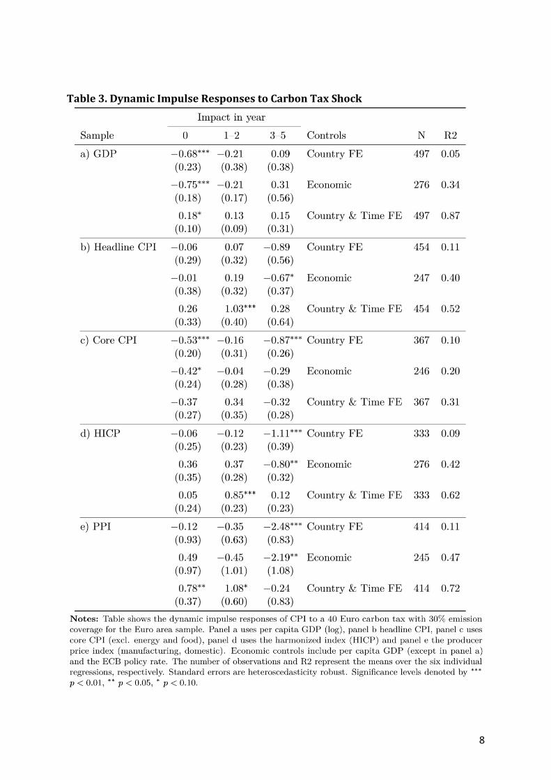
The dynamic effects are summarized in Table 3. We begin with the impulse responses for GDP per capita, in panel a. The first row includes only a country fixed effect, the second row adds the ECB’s policy rate as a control variable, and the third row includes country and time fixed effects. Impulse responses in the first two rows point to a negative and statistically significant effect on impact that dissipates over time. When adding a time fixed effect (row 3), the dynamic responses switch signs in the five years after the tax implementation. However, only the contemporaneous impact is statistically significant (at the 10% confidence level).

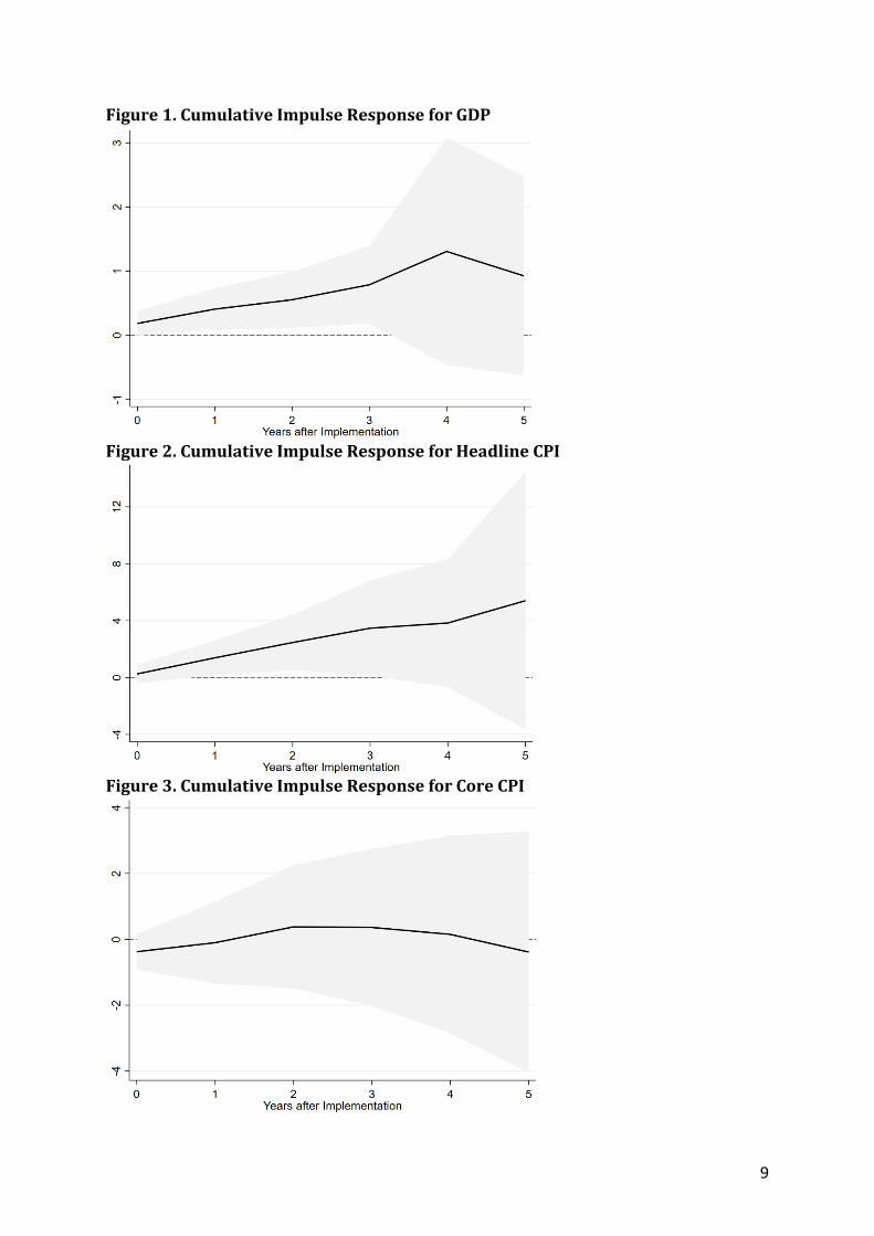
Quantitatively, our findings suggest that a €40 carbon tax applied on 30% of emissions leads to an increase of per capita GDP of 0.18 percentage points (p.p.) contemporaneously, 0.13 p.p. on average in the following two years and an average increase of 0.15 p.p. in the final three years. We illustrate the impulse response function of GDP per capita, including 95% confidence bands, graphically in Figure 1. These responses are broadly consistent with Metcalf (2019) and Metcalf and Stock (2020), who find a modest positive response of GDP.

Panel b shows the results for headline CPI. When including country and time fixed effects (row 3), the impulse response is positive and statistically significant at the 1 percent confidence level in the two years following the carbon tax shock. In the medium-term (years 3-5), the response remains positive but does not exceed its standard errors. The estimated effects echo prior results by Konradt and Weder di Mauro (2021), that countries without independent monetary policy seem to experience more inflationary responses after carbon tax enactments.

7

In quantitative terms, the enactment of a €40 carbon tax with 30% emission coverage is estimated to lead to an increase in headline CPI by 0.26 index points (in the same year), increasing to 1.03 index points (on average) over the next two years and an average increase of 0.28 index points in the following three years. We depict the cumulative impulse response in Figure 2. Five years removed, the carbon tax enactment leads to an increase of core CPI by four index points, which is, however, not statistically significant.

Next, we turn to core CPI (excluding energy and food) in panel c. The impulse responses are overwhelmingly negative, albeit not statistically significant when including country and time fixed effects. The deflationary response stands in contrast to the results on headline CPI (panel b) but confirms previous results by Konradt and Weder di Mauro (2021). The authors document that while energy prices tend to increase, prices of other goods, primarily non-tradable, tend to fall after a carbon tax implementation.

The estimated impulse responses imply a contemporaneous fall of 0.37 index points, followed by an increase in core CPI of 0.34 index points in each of the next two years and a further decline of 0.32 index points, on average in the final three years following the enactment of a €40 carbon tax with 30% coverage. Once more, we illustrate the cumulative response of core CPI to the carbon tax shock in Figure 3.

As a robustness check, we use the harmonized price index (HICP) in panel d. The last row (including country and time fixed effects) highlights that the impulse response is nearly identical to the headline CPI response. That is, we find a positive and statistically significant (at the 1% confidence level) response of HICP in the first two years after a carbon tax enactment.

Finally, we test whether producer prices, measured through PPI, react similarly to CPI. The dynamic responses (panel e) show a precisely estimated positive effect on impact and in the two succeeding years after a carbon tax when including country and time fixed effects. The estimated impulse responses are quantitatively large, also in comparison to CPI (panel b). This result could by indicative of producers shouldering most of the burden associated with a carbon tax, rather than passing it on to consumers.

Our reported findings survive a battery of robustness checks. First, the coefficients are of similar size when excluding the period before 2000 and using a sample comprising only of initial member countries. Second, we find similar results when denominating all variables in real USD instead of EUR/DM. Lastly, our findings remain unchanged when using the ECB shadow rate (Wu and Xia 2016) instead of the actual policy rate.

8

Table 3. Dynamic Impulse Responses to Carbon Tax Shock

9

Figure 1. Cumulative Impulse Response for GDP

Figure 2. Cumulative Impulse Response for Headline CPI

Figure 3. Cumulative Impulse Response for Core CPI

10

4. The G-Cubed Model

This section outlines a new European version of the G-Cubed model used to explore the impact of two alternative monetary rules for the ECB under a range of different climate-related shocks and climate policy changes. These are discussed in detail in the following sections.

The G-Cubed model is a global, multisector model, which has been designed to evaluate climate policy and has been used to estimate the impact of environmental shocks (see McKibbin and Wilcoxen 2013 and McKibbin et al. 2018 and 2020, IMF 2020). The model has been modified in this paper in several ways to explore the European setting better. We incorporate a policy rule for the ECB based on Hartmann and Smets (2018) and Orphanides and Wieland (2013) by making the monetary policy reaction function more forward-looking. We have also modified the European version to represent the Euro area rather than all of Western Europe which has been the aggregation in previous climate papers using G-Cubed. The Euro area in this new model version is Germany, France, Italy, Spain, Netherlands, Belgium, Luxemburg, Ireland, Greece, Austria, Portugal, Finland, Cyprus, Estonia, Latvia, and Lithuania. The countries removed from the Western Europe aggregation (which included United Kingdom amongst others) have been reallocated to the Rest of the OECD and the rest of the world.

There are ten regions and 20 sectors in the version of the model (version GGG20Nv161) used in this paper. These are contained in Table 4.

Table 4. Regions in the G-Cubed model

Region Code Region Description AUS Australia CHN China EUR Euro Area IND India JPN Japan OPC Oil-Exporting developing countries OEC Rest of the OECD ROW Rest of the World RUS Russian Federation USA United States

The sectors in the model are set out in Table 5.

11

Table 5. Sectors in the G-Cubed model

Number Sector Name Note 1 Electricity delivery

Energy Sectors Other than Generation

2 Gas extraction and utilities 3 Petroleum refining 4 Coal mining 5 Crude oil extraction 6 Construction

Goods and Services

7 Other mining 8 Agriculture and forestry 9 Durable goods 10 Nondurable goods 11 Transportation 12 Services 13 Coal generation

Electricity Generation Sectors

14 Natural gas generation 15 Petroleum generation 16 Nuclear generation 17 Wind generation 18 Solar generation 19 Hydroelectric generation 20 Other generation

The G-Cubed sectors 1-12 are aggregated from 65 sectors of the GTAP 10 database13. The electricity sector is further disaggregated into the electricity delivery sector (sector 1), which purchases inputs from 8 electricity generation sectors (sectors 13-20).

As outlined in Jaumont et al. (2021), there is a production structure for each sector within each country, as shown in Figure 6. CO2 emissions are measured through the burning of fossil fuels in energy generation.

13 See Aguiar et al. (2019).

12

Figure 4. Production and consumption structure for each sector in the G-Cubed model

Note that the elasticities of substitution between capital, labor, energy, and materials and between the sub nests within each sector are estimated using US data14. The parameter for input shares in the CES production function is taken from the latest input-output tables in the GTAP 10 database.

The model completely accounts for stocks and flows of physical and financial assets. For example, budget deficits accumulate into government debt, and current account deficits accumulate into foreign debt. The model imposes an intertemporal budget constraint on all households, firms, governments, and countries. Thus, a long-run stock equilibrium obtains by adjusting asset prices, such as the interest rate for government fiscal positions or the real exchange rates for the balance of payments. However, the adjustment towards the long-run equilibrium of each economy can be slow, occurring over a century.

Households and firms in G-Cubed must use money issued by central banks for all transactions. Thus, central banks in the model set short-term nominal interest rates to target macroeconomic outcomes (such as inflation, unemployment, exchange rates, etc.) based on Henderson-McKibbin-Taylor monetary rules15. These monetary rules approximate actual monetary regimes in each country or region in the model. They tie

14 These elasticities are assumed to be the same across countries but different across sectors. In other words, the degree of substitution across input in production is a sector are different across sectors but are the same for the same sector in different countries. 15 See Henderson and McKibbin (1993), Taylor (1993), Orphanides (2003).

13

down the long-run inflation rates in each country and allow short-term adjustment of policy to smooth fluctuations in the real economy.

Nominal wages are sticky and adjust over time based on country-specific labor contracting assumptions. Firms hire labor in each sector up to the point that the marginal product of labor equals the real wage defined in terms of the output price level of that sector. Any excess labor enters the unemployed pool of workers. Unemployment or the presence of excess demand for labor causes the nominal wage to adjust to clear the labor market in the long run. In the short run, unemployment can arise due to structural supply shocks or changes in aggregate demand in the economy.

Rigidities prevent the economy from moving quickly from one equilibrium to another. These rigidities include nominal stickiness caused by wage rigidities, lack of complete foresight in the formation of expectations, cost of adjustment in investment by firms with physical capital being sector-specific in the short run. With these rigidities and monetary and fiscal authorities following particular monetary and fiscal rules, short-term adjustment to economic shocks can be very different from the long-run equilibrium outcomes. Note that each sector in each country has a capital stock that is based on putty-clay technology. It is costly to move installed physical capital between sectors. This stickiness is an important aspect of the cost of decarbonizing economies, given current energy systems and technologies for using energy.

The model incorporates heterogeneous households and firms. Firms are modeled separately within each sector. The model distinguishes between consumers and firms that base their decisions on forward-looking expectations and those that follow more straightforward rules of thumb, which are optimal in the long run but not necessarily in the short run.

The fiscal rule in the model varies across model versions. In this paper’s version of the model, we assumed an endogenous budget deficit with lump-sum taxes on households adjusted gradually over time to cover any incremental interest payments to ensure fiscal sustainability. Thus, the level of government debt can permanently change in the long run with the change in debt to GDP equal to the ratio of the long-run fiscal deficit to the long-run real growth rate of the economy. Based on the extensive literature, including previous studies with the G-Cubed model, we know that the assumption of how carbon tax revenue is used can have significant macroeconomic implications16. Rather than show a range of assumptions in this paper, we assume that the tax revenue is used to reduce the fiscal deficit across all central bank monetary regimes.

16 See McKibbin W. J., Morris, A., Wilcoxen P. J., and Y. Cai (2015) and McKibbin W. J., Morris, A., Wilcoxen P. J. and L. Liu (2018).

14

Optimal Monetary Policy

There is extensive literature on the optimal rules for monetary policy17. Monetary policy rules for interest rates responding to intermediate targets range from money targeting, exchange rate targeting, commodity price targeting, inflation targeting, price level targeting, nominal income targeting, nominal income growth targeting, and rules explicitly embodying tradeoffs between variables such as Henderson-McKibbin Taylor Rules. The main insights from this literature relevant for this paper are that most monetary rules handle demand shocks well, but some rules perform poorly in the face of supply shocks and changes in country risk18.

Since climate shocks and climate policy changes tend to be supply shocks, many of these monetary regimes will not be helpful during a climate transition. While the modeling framework in this paper can simulate each of these monetary rules, the focus in this paper will be on the types of rules likely to be relevant for climate transition scenarios. Other applicable monetary rules which would also be interesting to explore further are price-level targeting and nominal income rules. However, due to space limitations, these will be explored in future research.

The subset of monetary rules that we focus on are rules that incorporate output and inflation tradeoffs, such as Henderson McKibbin Taylor Rules. The focus will further narrow down to the Hartmann-Smets (2018) rule, which the authors argued to be a good empirical representation of the ECB policy rule over recent decades. We then focus on the relevance of the tradeoff between current versus future information in that rule.

Alternative Monetary Regimes for the ECB

We consider two alternative policy rules for the ECB.

The first is the Hartmann-Smets (2018) modification of the Orphanides-Wieland Rule (2013). These are forward-looking versions of the Henderson-McKibbin (1993) and Taylor (1993) rules. This rule is summarized in equation 1. We call this rule in the HS rule in the charts.

𝑖𝑖𝑡𝑡 = 𝑖𝑖𝑡𝑡−1 + 0.34 ∗ (𝜋𝜋𝑡𝑡,𝑡𝑡+1 − 𝜋𝜋�𝑡𝑡+1) + 0.4 ∗ �𝑔𝑔𝑡𝑡,𝑡𝑡+1 − �̅�𝑔𝑡𝑡+1� HS (1)

17 See Poole (1970), Taylor (1993), Henderson and McKibbin (1993), Orphanides (2013), Orphanides and Wieland (2013), Hartmann and Smets (2018) and the comprehensive study by Bryant et al. (1993). 18 Note that as Henderson and McKibbin (1993) and Bryant et al. (1993) point out, a fundamental assumption is the extent of wage and price stickiness in the economy.

15

Where 𝑖𝑖𝑡𝑡 is the policy interest rate, 𝜋𝜋𝑡𝑡,𝑡𝑡+1 is the expectation in period t of inflation in period t+1 (rationally expected from the model) and 𝑔𝑔𝑡𝑡,𝑡𝑡+1 is the growth rate in output in period t+1 expected in period t (the rational forecast from the model)

The second rule (equation 2) is an augmented rule similar to the Hartmann-Smets rule but with a weight on current period variables and a larger weight on one year ahead forecasts of inflation relative to target and output growth relative to the target. We call this rule the modified Hartmann-Smets (MHS)19 rule in the charts.

𝑖𝑖𝑡𝑡 = 𝑖𝑖𝑡𝑡−1 + 0.5 ∗ �0.34 ∗ (𝜋𝜋𝑡𝑡 − 𝜋𝜋�𝑡𝑡) + 0.4 ∗ (𝑔𝑔𝑡𝑡 − �̅�𝑔𝑡𝑡)� +0.5 ∗ (0.34 ∗ (𝜋𝜋𝑡𝑡,𝑡𝑡+1 − 𝜋𝜋�𝑡𝑡+1) + 0.4 ∗ �𝑔𝑔𝑡𝑡,𝑡𝑡+1 − �̅�𝑔𝑡𝑡+1� MHS (2)

We first solve the model from 2019 to 2100 using exogenous population projections, sectoral productivity growth rates by sector and country, and projections of energy efficiency improvements based on historical experience. The key inputs into the baseline are the initial dynamics from 2018 to 2019 (the evolution of each economy from 2018 to 2019) and subsequent projections from 2019 onwards for productivity growth rates by sector and country. Sectoral output growth from 2019 onwards is driven by labor force growth and labor productivity growth. When solving the model to generate the baseline, we iteratively adjust temporal and intertemporal constants so that the model solution for 2019 replicates the database for 2019 (the latest data we have).

Each central bank scenario will be associated with a slightly different baseline in the initial decade because the monetary rule impacts the projection. We take this into account and present all results relative to the appropriate baseline.

5. Climate Shocks (Physical Risk) in the euro area

We now assess the macroeconomic consequences of climate risk. We follow Fernando, Liu, and McKibbin (2021) to consider a physical risk scenario that incorporates both chronic climate change and extreme climate events. The chronic climate change scenario is based on widely used climate scenarios (Representative Concentration Pathways, or RCP)20. Given this scenario, we use the results of Fernando, Liu, and McKibbin (2021). The authors calculate damage functions from that scenario RCP 4.5

19 In chapter 4 of Reichlin et al (2021) we implemented a modified Hartmann-Smets rule with 0.25 on current variables and 0.75 on future variables. It would be an interesting exercise to search over the degree of forward versus current information could minimize a central bank loss function. The values used in the current paper are chosen for illustrative purposes. 20 See van Vuuren, D. P., Edmonds, J., Kainuma, M., Riahi, K., Thomson, A., Hibbard, K., Hurtt, G. C., Kram, T., Krey, V., Lamarque, J. F., Masui, T., Meinshausen, M., Nakicenovic, N., Smith, S. J. & Rose, S. K. (2011).

16

due to chronic climate. The chronic climate risks considered in that study include sea-level rise, crop yield changes, heat-induced impacts on labor, and increased incidence of diseases.

This scenario is fed into the model through shocks to sectoral productivity and effective labor supplies. We then add to the chronic climate shocks (largely shocks to trends) our estimates of the probabilities of extreme climate events as calculated in Fernando et al. (2021). Fernando et al. (2021) estimate the future incidents of climate-related extreme events, including droughts, floods, heatwaves, cold waves, storms, and wildfires. These climate shocks are calculated for all countries in the model and will differ across sectors and countries.

Ideally, we would incorporate these extreme event shocks through stochastic simulations of the G-Cubed model to show the mean and variance of the variables of interest and better represent the uncertainty involved in climate shocks. A stochastic simulation approach will be undertaken in future research. For the current paper, we follow Fernando et al. (2021) and implement the mean of the shocks over time.

The response to European variables is explored given the two alternative monetary rules for the ECB.

Physical climate shocks are initially supply shocks. However, because the shocks change relative prices, asset returns, and estimates of capital valuation in different sectors and households’ evaluation of human wealth, the shocks also lead to endogenous changes in consumption and investment, which change aggregate and sectoral demand. The simulation assumes that in 2021 households, firms and governments in the model become aware of current and future climate shocks that are not in the baseline. The economic actors understand the RCP 4.5 scenario, expected extreme events, and impact productivity and effective labor supply. These shocks differ across sectors and countries.

Figures 5 to 8 contain results for the climate shocks for a range of macroeconomic and sectoral variables. Without any monetary response, the initial impact of the shock would likely be a fall in output in the most affected sectors (agriculture) and, therefore, a rise in relative prices of the most affected goods. Not surprisingly, agriculture has the most significant direct shock, but durable manufacturing output falls (not shown) because of the fall in investment in Europe. Durable goods feed into the creation of capital stock across the economy. However, in practice, many variables will change, such as equity prices, interest rates, expected investment returns, etc.

The figures contain two lines for each chart representing the results under the two monetary rules: the HS Rule (pink squares) and the MHS rule (green triangles). All results are expressed as either percent deviation, percentage point deviation, or percent

17

of GDP deviation from the baseline. The baseline under each monetary regime is different, so the relevant baseline is used in each case.

Figure 5 shows GDP, consumption, investment, the trade balance, the real effective exchange rate, and the real interest rate. The results indicate that the two alternative monetary rules have very different implications for the outcome of the climate shocks. Figure 5. Euro Area Aggregate Quantity Effects of a Global Climate Shock

18

Monetary policy is initially tightened under the HS rule because output growth is expected to recover in the year after. Thus expected GDP growth rises despite a significant fall in output in 2021. The fall in equity prices causes financial wealth to fall together with a fall in real wages. Consumption therefore falls. Under the HS rule, the rise in the interest rate causes human wealth to fall slightly more than under the MHS rule. The initial excessive monetary contraction exacerbates the climate shock by slowing the economy more and accentuating the fall in investment consumption. The slowdown also causes a slight improvement in the trade balance due to capital outflow. The MHS rule considers the sharp GDP drop in the current period and therefore does not tighten policy as much. There is still a slight tightening of policy by the ECB because the positive inflationary impact of the shock.

Inflation rises (Figure 6) in the MHS rule because of the relative price shock plus the relatively larger depreciation on the Euro feeds into imported prices for final goods and intermediate imported goods. Inflation falls under the HS rule because the tighter monetary policy reduces domestic prices and leads to an appreciation of the Euro causing import prices to fall. Using contemporaneous inflation in the policy rules leads to a smaller deviation of inflation and GDP from baseline under the MHS rule. The different inflation outcomes clearly show in the deviation of the aggregate price level, which is positive under the MHS rule but permanently negative under the HS rule. Most aggregate real variables are similar under both monetary regimes after several years because the monetary responses have passed through the economy. Note that the Euro/Dollar exchange rate reflects the permanent change in price levels under the two monetary regimes.

Sectoral results are shown in Figure 7. As expected, the permanent fall in aggregate GDP caused by the permanent supply shocks emanating from climate change leads to a decline across the sectors, although there are some interesting differences. Firstly, the most significant shocks occur in agriculture productivity, but the fall in investment across the economy has a disproportionate impact on the durable goods sector since this sector produces the goods that feed into the investment purchases of domestic firms. Durable goods are also important for exports, especially from Germany. Although we don’t show the global results, the adverse supply shocks are occurring globally, so there is also a global investment slump and implications for production supply chains globally. The construction sector is also hurt by the investment slowdown across the economy, reducing the demand for construction.

The sectoral results differ across the two monetary regimes. The additional tightening of monetary policy under the HS regime has a more significant negative impact on all sectors. The output loss is slightly more significant on construction and durable goods because these sectors are more sensitive to changes in real interest rates. Durable goods exports are also hurt by the appreciation of the Euro resulting from the tighter monetary policy.

19

Finally, it is interesting to observe how the monetary regimes change the tradeoff between inflation and GDP in the first year of the shock. This tradeoff is shown in Figure 8 for the two monetary regimes. The inflation change is on the vertical axis, and the change in GDP is on the horizontal axis. The HS rule has a larger output loss and deflation in response to the supply shock, whereas the MHS rule has a smaller output loss and higher inflation in response to the climate shock.

These results show that the choice of the monetary regime have a transitory impact on the short-term economic outcomes to climate shocks. It also seems important to use both current period information as well as expected future variables in the monetary policy rule.

Figure 6. Euro Area Inflation, Prices and Interest Rates under a global climate shock

20

Figure 7. Euro Area Sectoral Output under a Global Climate Shock

21

Figure 8. GDP/Inflation outcomes in year 1 of the climate Shock

6. European Climate Policy (Transition Risk) in the euro area

We now focus on transition risk. That is the impact of policies aimed at transitioning economies to a low carbon world. We focus in this section on European only carbon policy. Global carbon policy is explored in the following section.

We first consider the implications of implementing climate policy in the Euro area. We illustrate climate policy using a 50 euro per ton carbon tax rising at 3% per year. The revenue from the tax is used to reduce the Euro area-wide fiscal deficit. This tax is assumed to be understood by forward-looking households and firms as a precommitment by the European governments. As in the case of climate shocks above, we explore the macroeconomic and sectoral outcomes.

Our primary interest is studying how relative prices and inflation respond to the carbon tax under different assumptions about the reaction of the ECB. Given the relatively steep jump and continued increase in carbon costs, it is interesting to see if there might be higher inflation as a result.

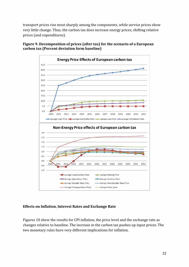
Figure 9 shows the decomposition of prices within the energy and non-energy components for the MHS rule (the results for both monetary rules are very similar). As expected, all energy prices respond to the carbon tax, most notably the price of coal which steadily increases from 25 up to 35 percent relative to baseline. Among sectors,

22

transport prices rise most sharply among the components, while service prices show very little change. Thus, the carbon tax does increase energy prices, shifting relative prices (and expenditures).

Figure 9. Decomposition of prices (after tax) for the scenario of a European carbon tax (Percent deviation form baseline)

Effects on Inflation, Interest Rates and Exchange Rate

Figures 10 show the results for CPI inflation, the price level and the exchange rate as changes relative to baseline. The increase in the carbon tax pushes up input prices. The two monetary rules have very different implications for inflation.

23

First, focus on the forward-looking HS rule. Following the carbon tax shock, GDP falls sharply in the first year, but in period t+1, output recovers with a higher growth rate but with GDP at a lower level (Figure 11). The HS rule balances lower inflation in period t+1 against higher growth relative to target in period t+1 and contracts monetary policy to offset the coming growth spike. Thus, rather than rising in period t, this type of monetary policy produces deflation in the first period. By mechanically looking through the shock to the period t+1, an entirely forward-looking ECB would “miss” the precise nature of the carbon tax shock in the initial period.

By contrast, the MHS rule is only partially forward-looking. It places a weight of 0.5 on first-period variables and 0.5 on period t+1 variables (using the HS relative weights on inflation and output growth in both periods). In this case, inflation would increase sharply in the year of the carbon price shock, as would initial output and consumption (Figure 11). Higher inflation under this monetary rule falls to about 0.1 percent p.a. in 2025 and eventually towards zero by the decade's end.

Figure 10. Euro area Inflation, Prices and Interest Rates under a European carbon tax (Percent deviation form baseline)

24

Both monetary rules control inflation within four years but note that the price level is very different under the two monetary rules. Under the MHS rule, the carbon tax will show up in a permanently higher price level. In contrast, the HS rule leads to a permanently lower price level, as prices do not fully recover from the initial deflationary shock.

Figure 11. Euro Area Aggregate Quantity Effects of a European carbon tax

25

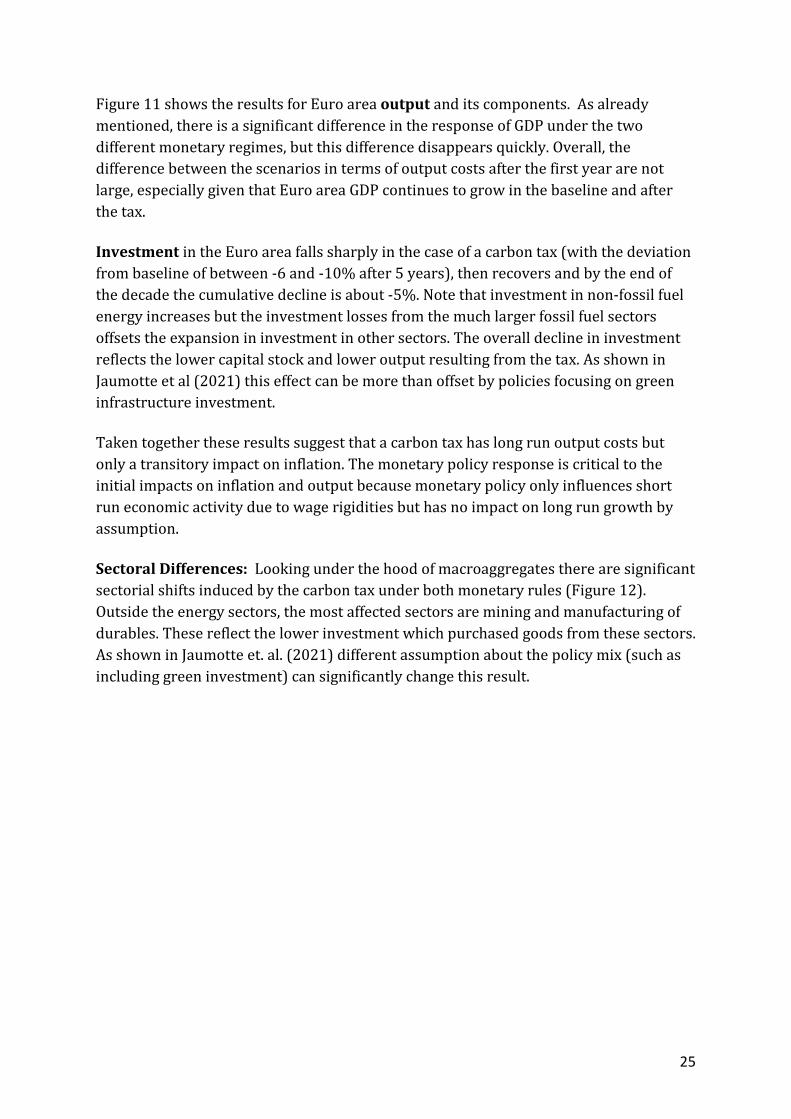
Figure 11 shows the results for Euro area output and its components. As already mentioned, there is a significant difference in the response of GDP under the two different monetary regimes, but this difference disappears quickly. Overall, the difference between the scenarios in terms of output costs after the first year are not large, especially given that Euro area GDP continues to grow in the baseline and after the tax.

Investment in the Euro area falls sharply in the case of a carbon tax (with the deviation from baseline of between -6 and -10% after 5 years), then recovers and by the end of the decade the cumulative decline is about -5%. Note that investment in non-fossil fuel energy increases but the investment losses from the much larger fossil fuel sectors offsets the expansion in investment in other sectors. The overall decline in investment reflects the lower capital stock and lower output resulting from the tax. As shown in Jaumotte et al (2021) this effect can be more than offset by policies focusing on green infrastructure investment.

Taken together these results suggest that a carbon tax has long run output costs but only a transitory impact on inflation. The monetary policy response is critical to the initial impacts on inflation and output because monetary policy only influences short run economic activity due to wage rigidities but has no impact on long run growth by assumption.

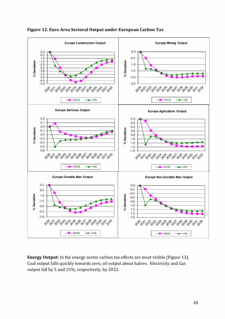
Sectoral Differences: Looking under the hood of macroaggregates there are significant sectorial shifts induced by the carbon tax under both monetary rules (Figure 12). Outside the energy sectors, the most affected sectors are mining and manufacturing of durables. These reflect the lower investment which purchased goods from these sectors. As shown in Jaumotte et. al. (2021) different assumption about the policy mix (such as including green investment) can significantly change this result.

26

Figure 12. Euro Area Sectoral Output under European Carbon Tax

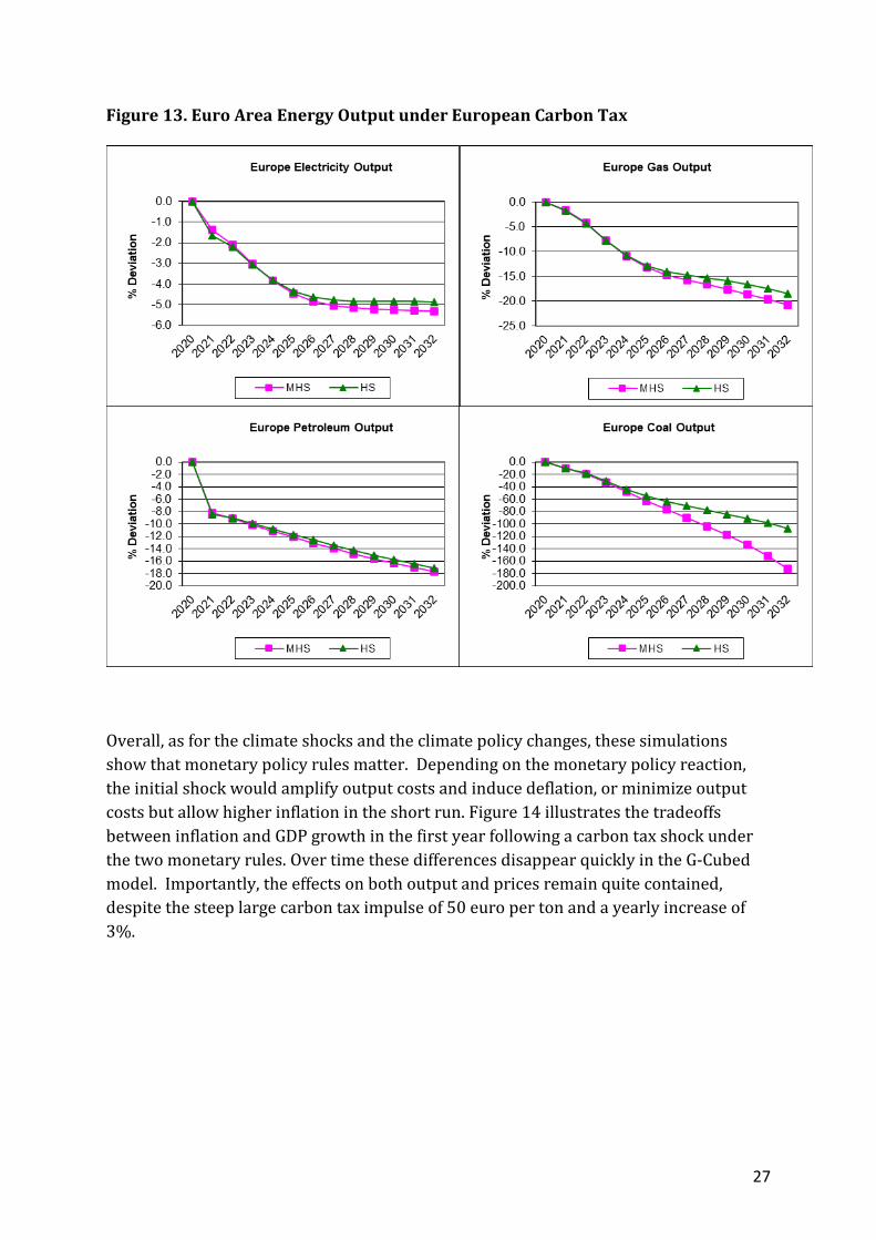
Energy Output: In the energy sector carbon tax effects are most visible (Figure 13). Coal output falls quickly towards zero, oil output about halves. Electricity and Gas output fall by 5 and 15%, respectively, by 2032.

27

Figure 13. Euro Area Energy Output under European Carbon Tax

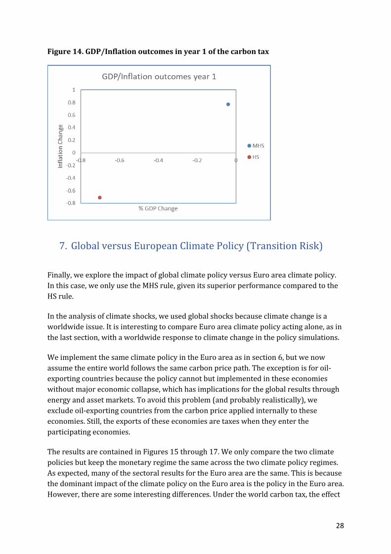
Overall, as for the climate shocks and the climate policy changes, these simulations show that monetary policy rules matter. Depending on the monetary policy reaction, the initial shock would amplify output costs and induce deflation, or minimize output costs but allow higher inflation in the short run. Figure 14 illustrates the tradeoffs between inflation and GDP growth in the first year following a carbon tax shock under the two monetary rules. Over time these differences disappear quickly in the G-Cubed model. Importantly, the effects on both output and prices remain quite contained, despite the steep large carbon tax impulse of 50 euro per ton and a yearly increase of 3%.

28

Figure 14. GDP/Inflation outcomes in year 1 of the carbon tax

7. Global versus European Climate Policy (Transition Risk)

Finally, we explore the impact of global climate policy versus Euro area climate policy. In this case, we only use the MHS rule, given its superior performance compared to the HS rule.

In the analysis of climate shocks, we used global shocks because climate change is a worldwide issue. It is interesting to compare Euro area climate policy acting alone, as in the last section, with a worldwide response to climate change in the policy simulations.

We implement the same climate policy in the Euro area as in section 6, but we now assume the entire world follows the same carbon price path. The exception is for oil-exporting countries because the policy cannot but implemented in these economies without major economic collapse, which has implications for the global results through energy and asset markets. To avoid this problem (and probably realistically), we exclude oil-exporting countries from the carbon price applied internally to these economies. Still, the exports of these economies are taxes when they enter the participating economies.

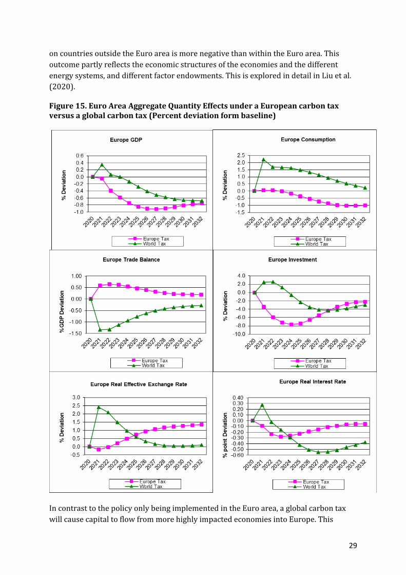
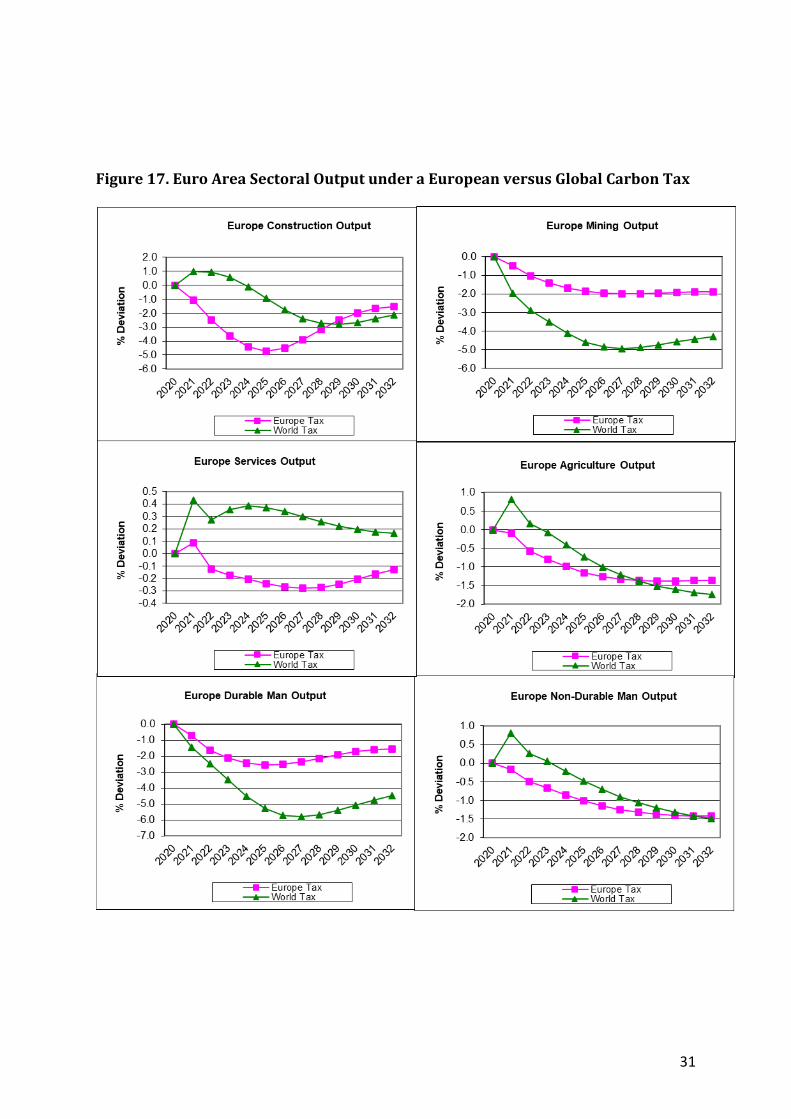
The results are contained in Figures 15 through 17. We only compare the two climate policies but keep the monetary regime the same across the two climate policy regimes. As expected, many of the sectoral results for the Euro area are the same. This is because the dominant impact of the climate policy on the Euro area is the policy in the Euro area. However, there are some interesting differences. Under the world carbon tax, the effect

29

on countries outside the Euro area is more negative than within the Euro area. This outcome partly reflects the economic structures of the economies and the different energy systems, and different factor endowments. This is explored in detail in Liu et al. (2020).

Figure 15. Euro Area Aggregate Quantity Effects under a European carbon tax versus a global carbon tax (Percent deviation form baseline)

In contrast to the policy only being implemented in the Euro area, a global carbon tax will cause capital to flow from more highly impacted economies into Europe. This

30

capital flow is reflected in a Eurozone trade deficit (Figure 15) rather than a trade surplus resulting from a Eurozone-only policy. This capital inflow tends to appreciate the Euro, which puts downward pressure on inflation through lower import prices for final goods and imported intermediate goods. The European terms of trade improve which raises income. Also, the relative loss of competitiveness of European exports is eliminated by the global policy. Thus, the decline in production at the sector level is reduced. Both consumption and investment in Europe are initially higher under the global policy compared to the Eurozone-only policy.

The problem facing the ECB in the two policy scenarios is different. Inflation is slightly higher (Figure 16) but the output is initially higher under the global policy and lower under the Euro area only policy.

Figure 16. Euro Area Inflation, Prices and Interest Rates under a European carbon tax versus a global carbon tax (Percent deviation form baseline)

31

Figure 17. Euro Area Sectoral Output under a European versus Global Carbon Tax

32

8. Summary and Conclusion

This paper explored the economic impact of physical climate risks and transition risks arising from a carbon tax for the Euro area economies.

We started by examining the historical effects of carbon pricing on output and inflation in the Euro area from 1985 to 2020. Compared to previous studies, this anaylsis considers a larger range of price indices, a longer period, and a narrower sample of countries consisting only of Euro area members. Nevertheless, broadly we find a similar pattern for the Euro area as in previous studies of Metcalf and Stock (2020) and Konradt and Weder di Mauro (2021). The effect of carbon taxation on GDP in the short run tends to be positive but imprecisely estimated. The short run effects on headline inflation are positive in the Euro area (while in larger samples they tend to be negative). Especially in the first two years after a tax introduction, we find that headline CPI and the HICP increased in some specifications by about 1 percent and 0.8 index points, respectively. After 3 years, inflation is contained. The impact on core inflation tended to be negative indicating that carbon taxes operated mostly by changing relative prices rather than affecting the overall price level, for a given monetary policy. Finally, we also find that producers have absorbed a part of the carbon tax since consumer prices increased less than producer prices.

We then proceed to examine the economy-wide and sectoral impacts of climate shocks and climate policies, in a new version of the global G-Cubed model, which focuses on the Euro area. We use this new model to explore physical climate risk (both underlying climate change and extreme climate events), transitional climate risk (through changes in climate policies), and climate policies applied only in the Euro area compared to a global policy response. We also explored the interaction of the climate shocks and the monetary policy regimes for the ECB, focusing on the degree of forward-lookingness of the monetary policy rule.

A first finding of the simulations is that the short run outcome from the various climate shocks depend significantly on the policy rule followed by the ECB. In particular, incorporating current and future information into the policy rule (which we call the modified Hartmann-Smets rule, MHS) leads to better inflation and output outcomes than a purely forward looking rule. Future work could explore the results across these weights to search for optimal weights on current and future information. The optimal weights will likely vary depending on the nature of the economic shocks and the economy's structure21.

21 See McKibbin and Sachs (1988) in the case of optimal simple exchange rate rules.

33

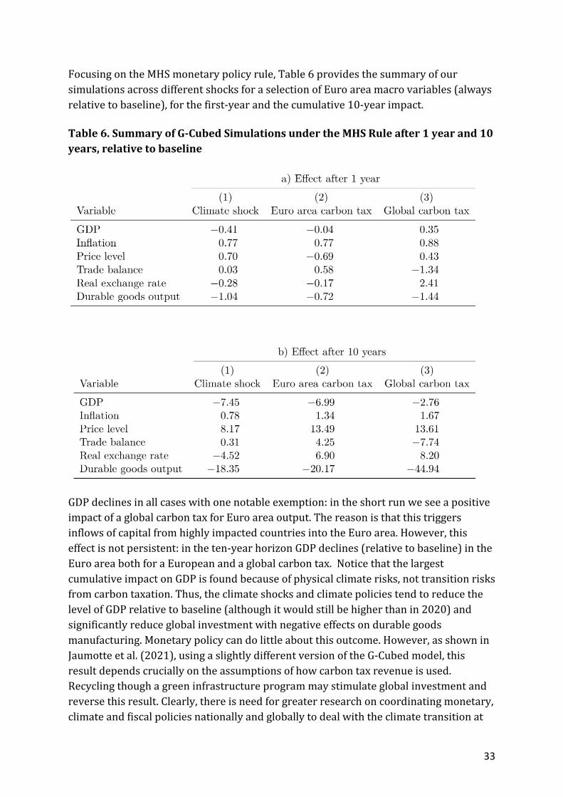
Focusing on the MHS monetary policy rule, Table 6 provides the summary of our simulations across different shocks for a selection of Euro area macro variables (always relative to baseline), for the first-year and the cumulative 10-year impact.

Table 6. Summary of G-Cubed Simulations under the MHS Rule after 1 year and 10 years, relative to baseline

GDP declines in all cases with one notable exemption: in the short run we see a positive impact of a global carbon tax for Euro area output. The reason is that this triggers inflows of capital from highly impacted countries into the Euro area. However, this effect is not persistent: in the ten-year horizon GDP declines (relative to baseline) in the Euro area both for a European and a global carbon tax. Notice that the largest cumulative impact on GDP is found because of physical climate risks, not transition risks from carbon taxation. Thus, the climate shocks and climate policies tend to reduce the level of GDP relative to baseline (although it would still be higher than in 2020) and significantly reduce global investment with negative effects on durable goods manufacturing. Monetary policy can do little about this outcome. However, as shown in Jaumotte et al. (2021), using a slightly different version of the G-Cubed model, this result depends crucially on the assumptions of how carbon tax revenue is used. Recycling though a green infrastructure program may stimulate global investment and reverse this result. Clearly, there is need for greater research on coordinating monetary, climate and fiscal policies nationally and globally to deal with the climate transition at

34

lowest economic cost. However, these findings also caution against “selling” a green transition as a growth program.

Inflation in the Euro area is contained in all shocks and the magnitude of the inflationary response is in line with our finding of the historical responses in the Euro area.

The Euro area trade balance and exchange rate respond very differently to a carbon tax if Europe acts unilaterally, compared with a global carbon tax. For the latter, the Euro area receives capital inflows (because it is less impacted relative to other countries in a global climate policy package), leading to an appreciation of the exchange rate and a trade deficit. Conversely, in the European carbon tax scenario capital flows out causing a slight exchange rate depreciation and a trade surplus which improves competitiveness despite the rise in the price of carbon on input prices. This is interesting, because it provides a counter argument to the logic of a Carbon Border Adjustment Mechansim (CBAM) as a way to adjust for the competitiveness effects of European carbon policy.

Finally, the cumulative contraction of durable goods manufacturing output is quantitatively large in all scenarios. It is largest on the global carbon policy because there is a global decline in investment in fossil fuel energy use and in carbon intensive industries. This contraction is not offset by an expansion in renewable intensive industries. With global investment weaker, the durable goods industry in the Euro area faces weaker demand from domestic industries and weaker export demand for durable investment goods. With Euro economies (especially Germany) a large exporter of durable goods, this impact is notable. It again highlights the importance of the role of a global infrastructure package to accompany the carbon pricing package as a way to rebalance the sectoral impacts of climate policy22.

The new ECB focus on climate change is a welcome and important development. As already argued in the ECB review, this will require developing new and more complex economic models. This paper demonstrates that there is already a research stream that can explore the interaction of monetary policy, fiscal policy and climate change. However, a great deal more research in this area is still needed. As the models developed over coming years will necessarily become more complex because of the complexity of a climate transition, a particularly useful direction would be to support model comparison exercises following the strategies of the Stanford Energy Modeling Forum (Fawcett et al 2018) and the Brookings Model Comparison Project (Bryant et al 1993).

22 See IMF (2020) and Jaumotte et al (2021) for analysis of this issue.

35

References

Andersson, M., C. Baccianti & Morgan, J. (2020), “Climate change and the macro economy”, ECB Occasional Paper Series.

Bang, E., Barrett, P., Banerjee, S., Bogmans, C., Brand, T., Carton, B., Eugstger, J., Fernandez, D. R., Jaumotte, F., Kim, J., Liu, W., McKibbin, W. J., Mohammad, A., Pugacheva, E., Tavares, M. M. & Voights, S. (2020), “Mitigating Climate Change”, World Economic Outlook, International Monetary Fund.

Basel Committee on Banking Supervision, BCBS (2020), “Climate-related financial risks: a survey on current initiatives”, BIS.

Bosello, F., Roson, R. & Tol, R. S. J. (2006), “Economy-wide estimates of the implications of climate change: Human health”, Ecological Economics, 58, 579-591.

Bosello, F., Roson, R. & Tol, R. S. J. (2007), “Economy-wide estimates of the implications of climate change: Sea level rise”, Environmental & Resource Economics, 37, 549-571.

Bryant, R., P. Hooper & Mann, C. (eds) (1993) “Evaluating Policy Regimes: New Research in Empirical Macroeconomics”, Brookings Institution.

Burke, M., S. M. Hsiang & Miguel, E. (2015), “Global Non-linear Effect of Temperature on Economic Production”, Nature 527:235–39.

Dell, M., Jones, B. F. & Olken, B. A. (2012), “Temperature Shocks and Economic Growth: Evidence from the Last Half Century”, American Economic Journal-Macroeconomics, 4, 66-95.

Dorland, C., Tol, R. S. J. & Palutikof, J. P. (1999), “Vulnerability of the Netherlands and Northwest Europe to storm damage under climate change - A model approach based on storm damage in the Netherlands”, Climatic Change, 43, 513-535.

Ebi, K. L. & Bowen, K. (2016), “Extreme events as sources of health vulnerability: Drought as an example”, Weather and Climate Extremes, 11, 95-102.

Eboli, F., Parrado, R. & Roson, R. (2010), “Climate-change feedback on economic growth: explorations with a dynamic general equilibrium model”, Environment and Development Economics, 15, 515-533.

Ekwezuo, C. S. & C. U. Ezeh, C. U. (2020), “Regional characterisation of meteorological drought and floods over west Africa”, Sustainable Water Resources Management, 6.

36

Fawcett, A., McFarland, J., Morris, A. C. & Weyant, J. P. (2018), “EMF 32 Study on U.S. Carbon Tax Scenarios”, Climate Change Economics Special Issue 01. World Scientific.

Fernando, R., Liu, W. & McKibbin, W. J. (2021), “Global Economic Impacts of Climate Shocks, Climate Policy and Changes in Climate Risk Assessment” Brookings Climate and Energy Economics Discussion Paper, March 31, 2021, CEPR Discussion paper DP16154 and CAMA working paper 37/2021.

Field, C. B., Barros, V., Stocker, T. F., Qin, D., Dokken, D. J., Ebi, K. L., Mastrandrea, M. D., Mach, K. J., Plattner, G. K., Allen, S. K. & Tignor, M. (2012), “A special report of working groups I and II of the intergovernmental panel on climate change. Managing the risks of extreme events and disasters to advance climate change adaptation”. United Nations Intergovernmental Panel on Climate Change.

Gollier, C. (2020), “The cost-efficiency carbon pricing puzzle”, TSE Working Paper No. 18-952.

Group of 30, G30 (2020), “Mainstreaming the Transition to Net Zero”.

Hallegatte, S. & Przyluski, V. (2010), “The economics of natural disasters: concepts and methods”, Washington D. C., The World Bank.

Hanson, C. E., Holt, T. & Palutikof, J. P. (2004), “An integrated assessment of the potential for change in storm activity over Europe: implications for insurance and forestry in the UK”, IT1.4 Final report. Tyndall Centre for Climate Change Research.

Hartmann, P. & Smets, F. (2018), “The European Central Bank’s Monetary Policy during its First 20 Years”, Brookings Papers on Economic Activity 2018(2), 1-146

Hausfather, Z. & Peters, G. P. (2020), “Emissions - the ’business as usual’ story is misleading”, Nature, 577, 618-620.

Henderson, D. W. & McKibbin, W. J. (1993), “A Comparison of Some Basic Monetary Policy Regimes for Open Economies: Implications of Different Degrees of Instrument Adjustment and Wage Persistence”, Carnegie-Rochester Conference Series on Public Policy, 39, 221-318.

Hsiang, S., Kopp, R., Jina, A., Rising, J., Delgado, M., Mohan, S., Rasmussen, D. J., Muir-Wood, R., Wilson, P., Oppenheimer, M., Larsen, K. & Houser, T. (2017), “Estimating economic damage from climate change in the United States”, Science, 356, 1362-1369.

IPCC (2021), “Climate Change: The Physical Science Basis. Contribution of Working Group I to the Sixth Assessment Report of the Intergovernmental Panel on Climate Change”, [Masson-Delmotte, V., P. Zhai, A. Pirani, S. L. Connors, C. Péan, S. Berger, N.

37

Caud, Y. Chen, L. Goldfarb, M. I. Gomis, M. Huang, K. Leitzell, E. Lonnoy, J. B. R. Matthews, T. K. Maycock, T. Waterfield, O. Yelekçi, R. Yu & Zhou, B. (eds.)]. Cambridge University Press. In Press.

Jaumotte, F., Liu, W. & McKibbin, W. J. (2021), “Mitigating Climate Change: Growth-friendly Policies to Achieve Net Zero Emissions by 2050”, IMF Working paper wp2021195. Washington DC. CAMA Paper 75/2021.

Jordà, O. (2005), “Estimation and Inference of Impulse Responses by Local Projections”, American Economic Review 95(1), 161-182.

Kjellstrom, T., Kovats, R. S., Lloyd, S. J., Holt, T. & Tol, R. S. (2009), “The direct impact of climate change on regional labor productivity”, Archives of Environmental & Occupational Health, 64, 217-227.

Kompas, T., Pham, V. H. & Che, T. N. (2018), “The Effects of Climate Change on GDP by Country and the Global Economic Gains From Complying With the Paris Climate Accord”, Earths Future, 6, 1153-1173.

Konradt, M. & Weder di Mauro, B. (2021), “Carbon Taxation and Inflation: Evidence from the European and Canadian Experience”, CEPR Discussion Paper No. 16396.

Krogstrup, S. & Oman, W. (2019), “Macroeconomic and Financial Policies for Climate Change Mitigation: A Review of the Literature”, IMF WP/19/185.

Leckebusch, G. C., Ulbrich, U., Fröhlich, L. & Pinto, J. G. (2007), “Property loss potentials for European mid-latitude storms in a changing climate”, Geophysical Research Letters, 34.

Liu, W., McKibbin, W. J., Morris, A. & Wilcoxen, P. J. (2020), “Global Economic and Environmental Outcomes of the Paris Agreement”, Energy Economics, 90, pp 1-17.

McKibbin, W. J. & Wilcoxen, P. J. (2013), “A Global Approach to Energy and the Environment: The G-cubed Model”, Handbook of CGE Modeling, Chapter 17, North Holland, pp 995-1068.

McKibbin, W. J. (1993) “Stochastic Simulations of Alternative Monetary Regimes in the MSG2 Model” in Bryant R., Hooper P., and C. Mann (1993) Evaluating Policy Regimes: New Research in Empirical Macroeconomics, Brookings Institution, pp 519-534.

McKibbin, W. J. (2012), “A New Climate Strategy Beyond 2012: Lessons from Monetary History”, 2007 (final version of the Shann Memorial Lecture), The Singapore Economic Review, Vol. 57, No. 3, 18 pages.

38

McKibbin, W. J. (2015), “Report 1: 2015 Economic modelling of international action under a new global climate change agreement.”, Report to Department of Foreign Affairs and Trade, 20.

McKibbin, W. J. & Sachs, J. (1988) “Comparing the Global Performance of Alternative Exchange Arrangements”, Journal of International Money and Finance, 7:4, pp 387 410

McKibbin, W. J. & Wilcoxen, P. J. (2002), “The Role of Economics in Climate Change Policy”, Journal of Economic Perspectives, vol 16, no 2, 107-129.

McKibbin, W. J., Morris, A., Wilcoxen P. J. & Panton, A. (2020), “Climate change and monetary policy: Issues for policy design and modelling”, Oxford Review of Economic Policy, 36(3), 579–603.

McKibbin, W. J., Morris, A., Wilcoxen P. J. & Liu, L. (2018), “The Role of Border Adjustments in a US Carbon Tax”, Climate Change Economics vol 9, no 1, 1-42.

McKibbin, W. J., Morris, A. C., Wilcoxen, P. J. & Cai, Y. (2012), “The Potential Role of a Carbon Tax in US Fiscal Reform”, The Brookings Institution. https://www.brookings.edu/wp-content/uploads/2016/06/carbon-tax-mckibbin-morriswilcoxen.pdf

Metcalf, G. (2019), “On the Economics of a Carbon Tax in the United States”, Brookings Papers on Economic Activity, Spring: 405-458.

Metcalf, G. & Stock, J. H. (2020), “Measuring the macroeconomic impact of carbon taxes”, AEA Papers and Proceedings, 110: 101-106.

Metcalf, G. (2019), “On the Economics of a Carbon Tax in the United States”, Brookings Papers on Economic Activity, Spring: 405-458.

NGFS (2019a), “First comprehensive report. A call for action. Climate change as a source of financial risk”, April.

NGFS (2019b), “Technical Supplement to the first comprehensive report”, July.

NGFS (2020), “On the implementation of sustainable and responsible investment practices in central banks’ portfolio management”, December.

NGFS (2020), “Climate Scenarios for Central Banks and Supervisors”, June.

Nordhaus, W. D. (2017), “Revisiting the social cost of carbon”, Proceedings of the National Academy of Sciences, Vol. 114, No. 7, pp. 1518-1523.

OECD (2015), “The Economic Consequences of Climate Change”, OCDE Publishing, Paris.

39

Orphanides, A. (2003), “Historical Monetary Policy Analysis and the Taylor Rule”, Board of Governors of the US Federal Reserve, Working Paper No. 2003-36.

Orphanides, A. & Wieland, V. (2013), “Complexity and Monetary Policy, International Journal of Central Banking”, vol. 9, pp. 167-203

Plagborg-Møller, M. & Wolf, C. K. (2021), “Local projections and VARs estimate the same impulse responses”, Econometrica 89(2), 955-980.

Poole, W. (1970), “Optimal Choice of Monetary Policy Instruments in a Simple Stochastic Macro Model” The Quarterly Journal of Economics Vol. 84, No. 2, May, pp. 197-216

Reichlin, L., Adam, K., McKibbin, W. J., McMahon, M., Reis, R., Ricco, G. & Weder di Mauro, B. (2021), “The ECB Strategy: The 2021 Review And Its Future”, Centre for Economic Policy Research, London.

Roson, R. & der Mensbrugghe, D. V. (2012), “Climate change and economic growth: Impacts and interactions”, International Journal of Sustainable Economy, 4, 270-285.

Roson, R. & Sartori, M. (2016), “Estimation of climate change damage functions for 140 regions in the GTAP9 database”, Policy Research Working Paper. Washington D. C.: World Bank Group.

Russo, S., Dosio, A., Graversen, R. G., Sillmann, J., Carrao, H., Dunbar, M. B., Singleton, A., Montagna, P., Barbola, P. & Vogt, J. V. (2014), “Magnitude of extreme heat waves in present climate and their projection in a warming world”, Journal of Geophysical Research-Atmospheres, 119, 12500-12512.

Schmitt, L. H., Graham, H. M. & White, P. C. (2016), “Economic Evaluations of the Health Impacts of Weather-Related Extreme Events: A Scoping Review”, International Journal of Environmental Research and Public Health, 13(11).

Sheng, Y. & Xu, X. P. (2019), “The productivity impact of climate change: Evidence from Australia’s Millennium drought”, Economic Modelling, 76, 182-191.

Sillmann, J., Thorarinsdottir, T., Keenlyside, N., Schaller, N., Alexander, L. V., Hegerl, G., Seneviratne, S. I., Vautard, R., Zhang, X. B. & Zwiers, F. W. (2017), “Understanding, modeling and predicting weather and climate extremes: Challenges and opportunities”, Weather and Climate Extremes, 18, 65-74.

Stern, N. (2007), “The economics of climate change: the Stern review”.

Taylor, J.B. (1993), “Discretion Versus Policy Rules in Practice”, Carnegie-Rochester Conference Series on Public Policy, 39(1), North Holland, December, pp. 195-214

40

van der Ploeg, F. (2020), “Macro-Financial Implications of Climate Change and the Carbon Transition”, ECB Sintra Conference Proceedings.

van der Ploeg, F. & Rezai, A. (2019), “The agnostic’s response to climate deniers: Price carbon”, European Economic Review, 111, 70-84.

van der Ploeg, F. & Rezai, A. (2020), “The risk of policy tipping and stranded carbon assets”, Journal of Environmental Economics and Management, 100.

van Vuuren, D. P., Edmonds, J., Kainuma, M., Riahi, K., Thomson, A., Hibbard, K., Hurtt, G. C., Kram, T., Krey, V., Lamarque, J. F., Masui, T., Meinshausen, M., Nakicenovic, N., Smith, S. J. & Rose, S. K. (2011), “The representative concentration pathways: an overview”, Climatic Change, 109, 5-31.

Wang, Z. L. & Cao, L. (2011), “Analysis on characteristics of droughts and floods of Zhengzhou City based on SPI in recent 60 years”, Journal of North China Institute of Water Conservancy and Hydroelectric Power, 6.

Weitzman, M. L. (2011), “Fat-tailed uncertainty in the economics of catastrophic climate change”, Review of Environmental Economics and Policy, 5, 275-292.

Wu, J. Z. & Xia, F. D. (2017), “Measuring the macroeconomic impact of monetary policy at the zero lower bound”, Journal of Money, Credit and Banking 48(2-3), 253-291.

41

Appendix Figure I

NGFS 2020

Climate Senarios for Central Banks and Supervisors