WP/12/166

Peru: Monetary and Exchange Rate Policies, 1930–1980

Gonzalo Pastor

© 2012 International Monetary Fund WP/12/166

IMF Working Paper

African Department

Peru: Monetary and Exchange Rate Policies, 1930–1980

Prepared by Gonzalo Pastor1

Authorized for Distribution by Calvin McDonald

June 2012

Abstract

This paper reviews monetary and exchange rate policies in Peru in 1930-80. The review covers major transformations to the world economy, including the post-1929 crash and WWII, and changing economic paradigms, such as the collapse of the gold standard and the rise and fall of the Bretton Woods system of fixed exchange rates. The analysis emphasizes the lasting partnership between Peruvian policymakers and the Bretton Woods institutions, while stressing the local authorities’ ownership of final policy decisions. The review shows that, in general, during the fifty year period under analysis, the Peruvian authorities sought to deliver nominal exchange rate stability, even at the cost of introducing market distortions and/or incurring heavy losses in international reserves.

JEL Classification Numbers: E5, F4, N1

Keywords: Peru monetary and exchange rate policies; Bretton Woods system; Polak model

Author’s E-Mail Address:gpastor@imf.org

1 The author is most grateful to Shane Hunt for his challenging comments on this paper. Thanks are also due to Carlos Contreras, Javier Hamann, Alfonso Quiroz, Miguel Savastano, Jorge Vega, Richard Webb and the staff of the Economics Studies Department at the Central Reserve Bank of Peru (BCRP) for their suggestions on how to improve earlier versions of this paper. Jenny DiBiase’s and Karen Coyne’s support in editing and formatting this paper is most appreciated. The views expressed in this article are those of the author and do not necessarily represent those of the IMF or IMF policy. A shorter version of this paper, edited by Carlos Contreras, will be published in Spanish in Volume V of Compendio de Historia Económica del Perú, to be issued by the BCRP, the Instituto de Estudios Peruanos , and the Pontificia Universidad Católica del Perú in late-2012/early 2013.

This Working Paper should not be reported as representing the views of the IMF. The views expressed in this Working Paper are those of the author(s) and do not necessarily represent those of the IMF or IMF policy. Working Papers describe research in progress by the author(s) and are published to elicit comments and to further debate.

2

Contents Page

I. Introduction ..............................................................................................................................4 

II. Economic and Financial Antecedents to 1930 ........................................................................6 

III. Battling the Impact of the Great Depression and the Second World War, 1930-1945 ......11 

IV. From a Fixed to a Floating Exchange Rate Regime— An Arduous Transition, 1945/49 ..19 

V. Policy Challenges During President Odría’s Economic Bonanza and Afterward, 1950–1959....................................................................................................................................27 

VI. From a Unified Exchange System, Back to a Dual Exchange System, 1960–68 ..............39 

VII. Losing the Battle Against Inflation in a Context of Severe Macroeconomic Instability, 1969–1980..........................................................................................................................47 

VIII. Concluding Remarks ........................................................................................................58 

IX. Selected Bibliography .........................................................................................................62  Tables 1. Merchandise Exports and Imports, 1890–1929 .....................................................................7 2. Main Merchandise Exports, 1914–1939 ................................................................................8 3. Peruvian Pound (Lp) Exchange Rates, 1902–1929 ...............................................................9 4. Selected Economic Indicators, 1913–1980 ..........................................................................12 5. Contribution to Economic growth by Component of Aggregate Demand, 1930–1945 ......18 6. Contribution to Economic Growth by Component of Aggregate Demand, 1940–1955 .....22 7. Contribution to Economic Growth by Component of Aggregate Demand, 1950–62 .........33 8. Sectoral Districution of GDP, 1942–1959 ...........................................................................38 9. Contribution to Economic Growth by Component of Aggregate Demand, 1959–80 .........46 10. Sectoral Distribution of GDP, 1950–1978 .........................................................................46 11. Latin America: Real GDP Growth Rates, 1961–1970 .......................................................46 12. Savings-Investment Balance, Inflation and Economic Growth Rates, 1968–75 ...............50 13. Savings-Investment Balance, Inflation and Economic Growth Rates, 1975–80 ...............56  Figures 1. Nominal Exchange Rate against U.S. Dollar, 1934–1976 .....................................................4 2. Bilateral Real Exchange Rate with U.S. dollar, 1930–1981/ .................................................5 3. Food & Overall Annual Deflation Rates, 1927–1933 .........................................................13 4. Central Bank’s International Reserve Coverage, 1934–1959 ..............................................15 5. Total Imports and Real Exchange Rate Index, 1940–1950 .................................................16 6. Sources of Base Money Growth, 1941–45 ..........................................................................17 7. Sectoral Distribution of GDP, Average 1942–45 ................................................................18 8. Colombia: Sectoral Districution of GDP, 1945 ...................................................................19 

3

9. Sources of Base Money Growth, 1945–1949 ......................................................................23 10. Velocity of Money & Private Sector Credit Growth, 1942–1958 .....................................24 11. Exchange Rates, Jan 1949–June 1950 ...............................................................................25 12. Savings – Investment Balance ...........................................................................................27 13. Total Imports and Real Exchange Rate Index, (1934=100) ..............................................35 14. Cost of Living & Nominal Exchange Rate, 1950–59 ........................................................35 15. Sources of Base Money Growth, 1950–59 ........................................................................37 16. Velocity of Money & Private Sector Credit Growth, 1959–1969 .....................................39 17. RER Index & Average Monthly Imports, 1957–1968 .......................................................44 18. Sources of Base Money Growth, 1962–1967 ....................................................................45 19. Economic Growth & Inflation Rates, 1968–1980 .............................................................47 20. Total Imports and Real Exchange Rate Index (Index, 1934=100) ....................................50 21. Sources of Base Money Growth, 1969–74 ........................................................................52 22. Monthly Exchange Rate Devaluation, Jan. 1977–Dec. 1980 ............................................55 23. Sources of Base Money Growth, 1976–80 ........................................................................57 24. RER Index & Reserve coverage, 1968–80 ........................................................................58  Boxes 1. Relations with the IMF ........................................................................................................21 2. The Bretton Woods System .................................................................................................29 3. The Polak Model ..................................................................................................................30 4. President Odría’s Speech to the Nation ...............................................................................33 

4

I. INTRODUCTION

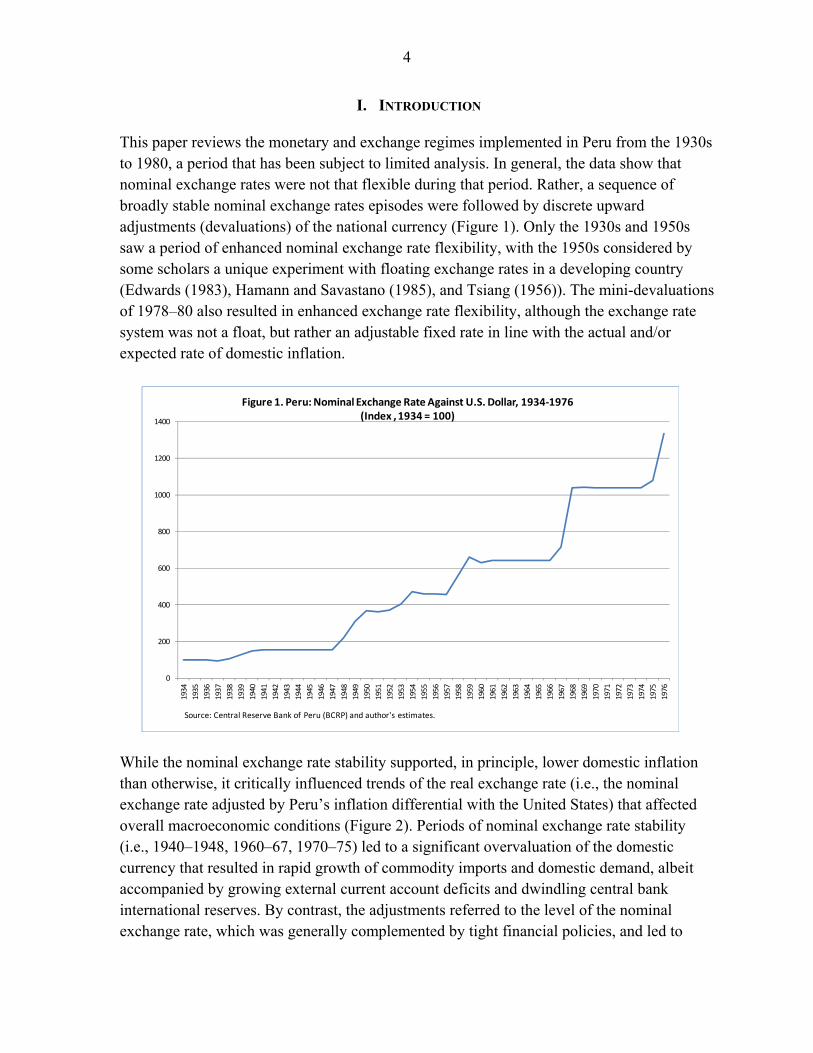
This paper reviews the monetary and exchange regimes implemented in Peru from the 1930s to 1980, a period that has been subject to limited analysis. In general, the data show that nominal exchange rates were not that flexible during that period. Rather, a sequence of broadly stable nominal exchange rates episodes were followed by discrete upward adjustments (devaluations) of the national currency (Figure 1). Only the 1930s and 1950s saw a period of enhanced nominal exchange rate flexibility, with the 1950s considered by some scholars a unique experiment with floating exchange rates in a developing country (Edwards (1983), Hamann and Savastano (1985), and Tsiang (1956)). The mini-devaluations of 1978–80 also resulted in enhanced exchange rate flexibility, although the exchange rate system was not a float, but rather an adjustable fixed rate in line with the actual and/or expected rate of domestic inflation.

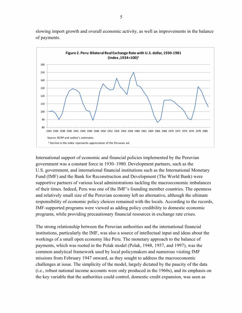
While the nominal exchange rate stability supported, in principle, lower domestic inflation than otherwise, it critically influenced trends of the real exchange rate (i.e., the nominal exchange rate adjusted by Peru’s inflation differential with the United States) that affected overall macroeconomic conditions (Figure 2). Periods of nominal exchange rate stability (i.e., 1940–1948, 1960–67, 1970–75) led to a significant overvaluation of the domestic currency that resulted in rapid growth of commodity imports and domestic demand, albeit accompanied by growing external current account deficits and dwindling central bank international reserves. By contrast, the adjustments referred to the level of the nominal exchange rate, which was generally complemented by tight financial policies, and led to

0

200

400

600

800

1000

1200

1400

1934

1935

1936

1937

1938

1939

1940

1941

1942

1943

1944

1945

1946

1947

1948

1949

1950

1951

1952

1953

1954

1955

1956

1957

1958

1959

1960

1961

1962

1963

1964

1965

1966

1967

1968

1969

1970

1971

1972

1973

1974

1975

1976

Figure 1. Peru: Nominal Exchange Rate Against U.S. Dollar, 1934-1976 (Index , 1934 = 100)

Source: Central Reserve Bank of Peru (BCRP) and author's estimates.

5

slowing import growth and overall economic activity, as well as improvements in the balance of payments.

International support of economic and financial policies implemented by the Peruvian government was a constant force in 1930–1980. Development partners, such as the U.S. government, and international financial institutions such as the International Monetary Fund (IMF) and the Bank for Reconstruction and Development (The World Bank) were supportive partners of various local administrations tackling the macroeconomic imbalances of their times. Indeed, Peru was one of the IMF’s founding member countries. The openness and relatively small size of the Peruvian economy left no alternative, although the ultimate responsibility of economic policy choices remained with the locals. According to the records, IMF-supported programs were viewed as adding policy credibility to domestic economic programs, while providing precautionary financial resources in exchange rate crises. The strong relationship between the Peruvian authorities and the international financial institutions, particularly the IMF, was also a source of intellectual input and ideas about the workings of a small open economy like Peru. The monetary approach to the balance of payments, which was rooted in the Polak model (Polak, 1948, 1957, and 1997), was the common analytical framework used by local policymakers and numerous visiting IMF missions from February 1947 onward, as they sought to address the macroeconomic challenges at issue. The simplicity of the model, largely dictated by the paucity of the data (i.e., robust national income accounts were only produced in the 1960s), and its emphasis on the key variable that the authorities could control, domestic credit expansion, was seen as

80

90

100

110

120

130

140

150

160

1934 1936 1938 1940 1942 1944 1946 1948 1950 1952 1954 1956 1958 1960 1962 1964 1966 1968 1970 1972 1974 1976 1978 1980

Figure 2. Peru: Bilateral Real Exchange Rate with U.S. dollar, 1930-1981 (Index ,1934=100)1

Source: BCRP and author's estimates.

1 Decline in the index represents appreciation of the Peruvian sol.

6

crucial for the understanding and correction of the balance of payments problems for which Fund assistance was being sought. The structure of the paper follows the time-line of major events that occurred in 1930–1980. Sections II and III summarize exchange and monetary policies during the transitions from a convertible gold coin standard to a gold bullion standard (i.e., gold coins do not circulate, but there is a fixed exchange rate in gold against circulating currency), and to a system of fixed parities following the outbreak of the Second World War. Sections IV and V cover the transition from a fixed to a floating exchange rate system under the Odría administration—including the implementation of the first set of Stand-By Arrangement programs (SBAs) agreed to with the IMF—and the monetary and exchange rate policies undertaken during the economic bonanza of the 1950s and immediately afterwards. Sections VI and VII cover policies under the Belaúnde administration and those applied under the leadership of Generals Velasco and Morales Bermudez through the end of the 1970s. Section VIII and IX include some concluding remarks and a selected list of bibliographical sources. The data sources and information used in the preparation of this paper are varied. The leading effort by the Central Reserve Bank of Peru in compiling and summarizing minutes of its own executive board discussions (Banco Central de Reserva del Perú, 1999) has been complemented by IMF staff reports (referred to as SMs or EBS in the bibliography) and minutes from IMF Executive Board meetings (referred to as EBM in the bibliography) that are now available to the public. An array of economic publications listed in the bibliography has also provided information and enthusiasm to produce this limited summary of a rich period of economic policy in Peru. All errors, of course, remain with this author.

II. ECONOMIC AND FINANCIAL ANTECEDENTS TO 1930

Little robust macroeconomic data are available for the early 1900s, although obtainable information indicates that economic and export growth was strong and inflation was in the low single-digits in 1901–1914. Domestic investment was mainly financed by private domestic savings, while rising international trade taxes provided resources to cover a small public investment program. Peru was not a net borrower of international savings to finance its domestic investment, but rather a creditor to the rest of the world because exports of goods and services (and income) were higher than imports.

7

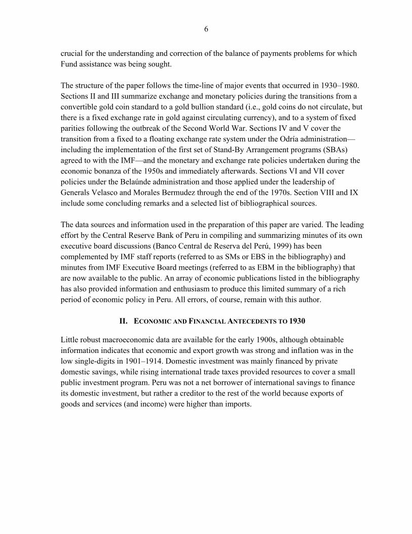
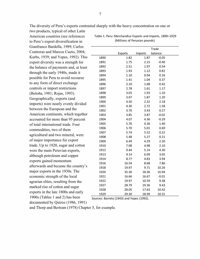
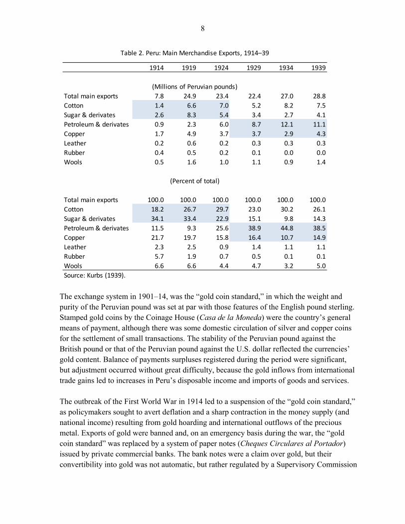
The diversity of Peru’s exports contrasted sharply with the heavy concentration on one or two products, typical of other Latin American countries (see references to Peru’s export diversification in Gianfranco Bardella, 1989; Carlos Contreras and Marcos Cueto, 2004; Kurbs, 1939; and Yepes, 1992). This export diversity was a strength for the balance of payments and, at least through the early 1940s, made it possible for Peru to avoid recourse to any form of direct exchange controls or import restrictions (Boloña, 1981; Rojas, 1993). Geographically, exports (and imports) were nearly evenly divided between the European and the American continents, which together accounted for more than 95 percent of total international trade. Four commodities, two of them agricultural and two mineral, were of major importance for export trade. Up to 1920, sugar and cotton were the main Peruvian exports, although petroleum and copper exports gained momentum afterwards and became the country’s major exports in the 1930s. The economic strength of the local agrarian elites, resulting from the marked rise of cotton and sugar exports in the late 1800s and early 1900s (Tables 1 and 2) has been documented by Quiroz (1986, 1991) and Thorp and Bertram (1978) Chapter 5, for example.

Exports Imports

Trade

balance

1890 1.82 1.87 -0.05

1891 1.75 2.15 -0.40

1892 2.51 1.97 0.54

1893 1.93 1.12 0.81

1894 1.10 0.94 0.16

1895 1.41 1.04 0.37

1896 2.10 1.68 0.42

1897 2.78 1.61 1.17

1898 3.03 1.93 1.10

1899 3.07 1.87 1.20

1900 4.50 2.32 2.18

1901 4.30 2.72 1.58

1902 3.70 3.43 0.27

1903 3.85 3.87 -0.02

1904 4.07 4.36 -0.29

1905 5.76 4.36 1.40

1906 5.70 5.01 0.69

1907 5.74 5.52 0.22

1908 5.48 5.27 0.21

1909 6.49 4.29 2.20

1910 7.08 4.98 2.10

1912 9.44 5.14 4.30

1913 9.14 6.09 3.05

1914 8.77 4.83 3.94

1916 16.54 8.68 7.86

1918 19.97 9.71 10.26

1920 35.30 18.36 16.94

1921 16.66 16.67 -0.01

1922 19.97 10.59 9.38

1927 28.79 19.36 9.43

1928 28.05 17.63 10.42

1929 29.30 18.99 10.31

Sources: Barreto (1943) and Yepes (1992).

(Millions of Peruvian pounds)

Table 1. Peru: Merchandise Exports and Imports, 1890–1929

8

The exchange system in 1901–14, was the “gold coin standard,” in which the weight and purity of the Peruvian pound was set at par with those features of the English pound sterling. Stamped gold coins by the Coinage House (Casa de la Moneda) were the country’s general means of payment, although there was some domestic circulation of silver and copper coins for the settlement of small transactions. The stability of the Peruvian pound against the British pound or that of the Peruvian pound against the U.S. dollar reflected the currencies’ gold content. Balance of payments surpluses registered during the period were significant, but adjustment occurred without great difficulty, because the gold inflows from international trade gains led to increases in Peru’s disposable income and imports of goods and services. The outbreak of the First World War in 1914 led to a suspension of the “gold coin standard,” as policymakers sought to avert deflation and a sharp contraction in the money supply (and national income) resulting from gold hoarding and international outflows of the precious metal. Exports of gold were banned and, on an emergency basis during the war, the “gold coin standard” was replaced by a system of paper notes (Cheques Circulares al Portador) issued by private commercial banks. The bank notes were a claim over gold, but their convertibility into gold was not automatic, but rather regulated by a Supervisory Commission

1914 1919 1924 1929 1934 1939

Total main exports 7.8 24.9 23.4 22.4 27.0 28.8

Cotton 1.4 6.6 7.0 5.2 8.2 7.5

Sugar & derivates 2.6 8.3 5.4 3.4 2.7 4.1

Petroleum & derivates 0.9 2.3 6.0 8.7 12.1 11.1

Copper 1.7 4.9 3.7 3.7 2.9 4.3

Leather 0.2 0.6 0.2 0.3 0.3 0.3

Rubber 0.4 0.5 0.2 0.1 0.0 0.0

Wools 0.5 1.6 1.0 1.1 0.9 1.4

Total main exports 100.0 100.0 100.0 100.0 100.0 100.0

Cotton 18.2 26.7 29.7 23.0 30.2 26.1

Sugar & derivates 34.1 33.4 22.9 15.1 9.8 14.3

Petroleum & derivates 11.5 9.3 25.6 38.9 44.8 38.5

Copper 21.7 19.7 15.8 16.4 10.7 14.9

Leather 2.3 2.5 0.9 1.4 1.1 1.1

Rubber 5.7 1.9 0.7 0.5 0.1 0.1

Wools 6.6 6.6 4.4 4.7 3.2 5.0

Source: Kurbs (1939).

Table 2. Peru: Main Merchandise Exports, 1914–39

(Percent of total)

(Millions of Peruvian pounds)

9

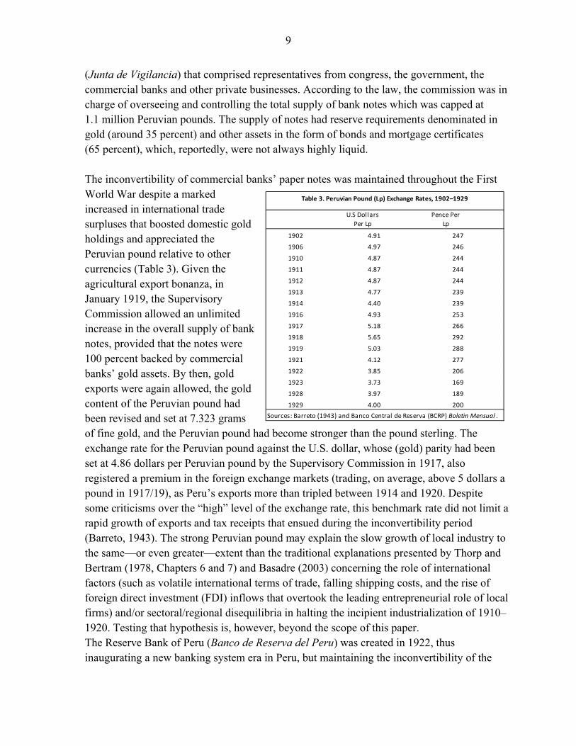
(Junta de Vigilancia) that comprised representatives from congress, the government, the commercial banks and other private businesses. According to the law, the commission was in charge of overseeing and controlling the total supply of bank notes which was capped at 1.1 million Peruvian pounds. The supply of notes had reserve requirements denominated in gold (around 35 percent) and other assets in the form of bonds and mortgage certificates (65 percent), which, reportedly, were not always highly liquid. The inconvertibility of commercial banks’ paper notes was maintained throughout the First World War despite a marked increased in international trade surpluses that boosted domestic gold holdings and appreciated the Peruvian pound relative to other currencies (Table 3). Given the agricultural export bonanza, in January 1919, the Supervisory Commission allowed an unlimited increase in the overall supply of bank notes, provided that the notes were 100 percent backed by commercial banks’ gold assets. By then, gold exports were again allowed, the gold content of the Peruvian pound had been revised and set at 7.323 grams of fine gold, and the Peruvian pound had become stronger than the pound sterling. The exchange rate for the Peruvian pound against the U.S. dollar, whose (gold) parity had been set at 4.86 dollars per Peruvian pound by the Supervisory Commission in 1917, also registered a premium in the foreign exchange markets (trading, on average, above 5 dollars a pound in 1917/19), as Peru’s exports more than tripled between 1914 and 1920. Despite some criticisms over the “high” level of the exchange rate, this benchmark rate did not limit a rapid growth of exports and tax receipts that ensued during the inconvertibility period (Barreto, 1943). The strong Peruvian pound may explain the slow growth of local industry to the same—or even greater—extent than the traditional explanations presented by Thorp and Bertram (1978, Chapters 6 and 7) and Basadre (2003) concerning the role of international factors (such as volatile international terms of trade, falling shipping costs, and the rise of foreign direct investment (FDI) inflows that overtook the leading entrepreneurial role of local firms) and/or sectoral/regional disequilibria in halting the incipient industrialization of 1910–1920. Testing that hypothesis is, however, beyond the scope of this paper. The Reserve Bank of Peru (Banco de Reserva del Peru) was created in 1922, thus inaugurating a new banking system era in Peru, but maintaining the inconvertibility of the

U.S Dollars

Per Lp

Pence Per

Lp

1902 4.91 247

1906 4.97 246

1910 4.87 244

1911 4.87 244

1912 4.87 244

1913 4.77 239

1914 4.40 239

1916 4.93 253

1917 5.18 266

1918 5.65 292

1919 5.03 288

1921 4.12 277

1922 3.85 206

1923 3.73 169

1928 3.97 189

1929 4.00 200

Sources: Barreto (1943) and Banco Central de Reserva (BCRP) Boletin Mensual .

Table 3. Peruvian Pound (Lp) Exchange Rates, 1902–1929

10

Peruvian pound through the end of the decade. Law #4500, of March 9, 1922, established the monetary authority to centralize the sources of monetary emission—which until then resided with the private commercial banks—and to provide a number of central bank functions existing in other countries. The latter included, among others, the provision of rediscount and advances to commercial banks, and the establishment of a clearing house for checks and intra-bank transactions. Currency emission by the monetary authority, in the form of central bank bills that replaced the commercial bank notes, gradually changed for a 100 percent gold backing to a more flexible (banking) system of 50 percent coverage, including gold and other liquid assets. The central bank law, however, retained the inconvertibility principle/policy of the Peruvian pound, noting that convertibility of central bank bills into gold required prior government consideration and approval, upon recommendation from the central bank board of directors.

In 1922–1929, the Peruvian pound gradually appreciated while the country became a net borrower of world savings to finance its expanding public investment program under the Leguía administration. A continuous rapid growth of volumes and values of cotton and sugar exports, combined with large public sector external borrowing, spurred the foreign exchange supply and led to an appreciation of the Peruvian pound against the U.S. dollar and pound sterling. However, interest payments on external public debt began to rise, offsetting the recorded external trade surpluses. The increase in external public debt was particularly marked during the 11-year (Oncenio) presidency of Augusto B. Leguía (1919–1930), whose ambitious investment program supported economic growth, but resulted in a rapid deterioration of the fiscal accounts and emerging pressures in the foreign exchange market starting in late-1927. Leguía’s public expenditure policies sought to respond to the needs of an emerging Peruvian middle class in terms of employment creation; the provision of basic police, health and education services; and the development of basic infrastructure to link the country’s distant regions (Contreras and Cueto, 2004, Chapter 6; Yepes, 1992, pages 49–52).

The 1920s closed with the collapse of Wall Street on “black” Thursday, October 24, 1929, which had a major impact on the American economy and economies around the world. A sharp contraction in bank credit and international capital flows accruing to raw material producers such as Peru, combined with a sharp fall in international commodity prices, led to a decline in export earnings and a depreciation of the Peruvian pound in the foreign exchange markets. Rising interest and amortization payments on external public debt further exacerbated the country’s balance of payments disequilibrium. On the domestic front, the U.S. financial crisis destroyed both wealth and employment in Peru and triggered a continuous decline in tax revenue collections and accompanying large fiscal deficits.

11

III. BATTLING THE IMPACT OF THE GREAT DEPRESSION AND THE SECOND WORLD WAR, 1930-1945

Overview

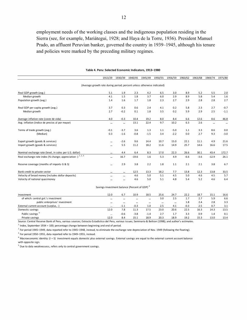
Relative to the early-1900s, 1930 to 1945 saw a deceleration in real GDP per-capita growth and ensuing fiscal and balance of payments deficits in a harsh international environment (Table 4, lower panel). In 1930–1939, the collapse of Wall Street and the subsequent worldwide deflation led to a sharp slowdown in Peru’s investment and overall economic activity, while the nominal exchange rate against the U.S. dollar depreciated marginally, because the impact from the deterioration in international trade conditions (that depreciated the exchange rate) was countered by the U.S. dollar depreciation in the international money markets following the decision by the United States to abandon the gold standard in 1933. From 1940 to 1945, the Second World War imposed further detrimental effects on multilateral trade, although several war-time bilateral trade and financing agreements with the U.S. government supported selected agricultural and mineral exports to the American market. Investment went up during this 6-year period largely reflecting the revival of local mining industry in response to premium international commodity prices. On the financial front, the Central Reserve Bank fixed the rate at 6.5 soles per dollar in mid-1940 and introduced exchange and trade controls that sought a broad matching of Peru’s imports to export receipts. By then, however, inflation was gradually increasing owing to large fiscal deficits that were mainly financed by central bank credit, because recourse to net external borrowing was practically impossible during this period on account of global financial uncertainties and Peru’s external debt service moratorium enacted under President Sánchez Cerro in May 1931. The rise in inflation due to rising monetary financing of the fiscal deficit led to an appreciation of the real exchange rate that boosted imports and unleashed emerging pressures on the central bank’s international reserve coverage. From a global perspective, Peru’s macroeconomic setbacks (in terms of growth and inflation) were minor compared with the massive destruction of physical and human capital (with 50 to 70 million fatalities) in Europe and Asia, as a result of the Second World War.

The underlying political project in 1930–1945 was a futile effort to re-establish the economic order in place in the early 1900s, before the presidency of Augusto B. Leguía (1919–1930). As such, the local agrarian elites, in cooperation with military leaders such as Luis Miguel Sánchez Cerro (1930–1933) and Oscar Benavides (1933–1939), sought to control the main political institutions, even at the cost of an emerging authoritarian state (see, for example, Contreras and Cueto,(2004, Chapter 7; and Yepes,1992). The international environment was good for local agriculture exporters in the final third of this period. They supplied cotton, rubber and selected minerals to support the American economy during the war years. However, the political intentions of the ruling group clashed with the middle classes’ economic and political demands for a more benevolent state, able to address the income and

12

employment needs of the working classes and the indigenous population residing in the Sierra (see, for example, Mariátegui, 1928; and Haya de la Torre, 1936). President Manuel Prado, an affluent Peruvian banker, governed the country in 1939–1945, although his tenure and policies were marked by the preceding military regimes.

1913/29 1930/39 1940/45 1945/49 1950/55 1956/59 1960/62 1963/68 1969/74 1975/80

Real GDP growth (avg.) 5.1 1.9 2.3 4.2 6.5 3.0 8.9 5.2 5.5 2.0

Median growth 4.1 1.5 1.8 3.7 6.0 2.9 8.9 5.8 5.4 1.6

Population growth (avg.) 1.4 1.6 1.7 1.8 2.3 2.7 2.9 2.8 2.8 2.7

Real GDP per capita growth (avg.) 3.7 0.3 0.6 2.4 4.1 0.2 5.8 2.3 2.7 -0.7

Median growth 2.7 -0.2 0.1 1.8 3.5 0.2 5.9 2.9 2.5 -1.1

Average inflation rate (coste de vida) 4.0 -0.3 10.4 19.2 8.0 8.4 6.6 12.6 8.6 46.8

Avg. inflation (indice de precios al por mayor) … … 13.1 22.4 9.7 10.2 6.3 2.6 … …

Terms of trade growth (avg.) -0.1 -3.7 3.6 1.3 1.1 -5.0 1.1 3.3 8.6 0.0

(Median) 0.3 -1.6 -0.8 -1.5 3.4 -2.2 0.0 2.7 9.3 -3.0

Export growth (goods & services) … -2.6 9.6 14.4 10.7 15.0 22.1 11.1 4.9 21.6

Import growth (goods & services) … 5.5 11.2 18.2 11.6 14.9 25.7 14.6 16.6 17.5

Nominal exchange rate (level, in soles per U.S. dollar) … 4.4 6.4 8.3 17.0 22.3 26.6 30.1 43.4 172.7

Real exchange rate index (% change; appreciation -) 1, 2, 3 … 16.7 -19.6 1.6 5.3 4.9 -6.6 -3.6 -12.9 26.1

Reserve coverage (months of imports G & S) … 2.9 3.8 2.2 1.8 1.1 2.1 2.1 3.8 6.7

Bank credit to private sector … … 12.5 13.3 18.2 7.7 13.8 12.3 13.8 33.5

Velocity of broad money (includes dollar deposits) … … 4.6 5.0 5.1 4.5 5.0 4.6 4.5 5.7

Velocity of national quasimoney … … 4.6 5.0 5.1 4.8 5.4 5.2 4.6 6.4

Investment 12.0 6.7 10.9 18.5 25.6 24.7 22.2 18.7 15.1 16.6

of which: central gvt.'s investment … … … … 3.0 2.5 1.7 2.7 5.9 6.6

public enterprises' investment … … … … … … 1.8 2.4 2.8 3.3

External current account (surplus, -) … -1.1 -0.3 1.0 2.5 4.1 -0.3 2.5 0.7 3.1

Domestic savings 12.0 7.8 11.3 17.5 23.0 20.6 22.5 16.3 14.3 13.5

Public savings 5 … -0.6 -3.8 -1.4 2.7 1.7 3.3 0.9 1.4 0.1

Private savings 12.0 8.4 15.1 18.9 20.3 18.9 19.2 15.3 13.0 13.4

Source: Central Reserve Bank of Peru, various sources; Extracto Estadistico del Peru, various issues; Seminario & Beltran (1998); and author's estimates.1 Index, September 1934 = 100; percentage change between beginning and end of period.2 For period 1945–1949, data reported refer to 1945–1948, instead, to eliminate the exchange rate depreciation of Nov. 1949 (following the floating).3 For period 1950–1955, data reported refer to 1949–1955, instead.4 Macroeconomic identity: (I = S) investment equals domestic plus external savings. External savings are equal to the external current account balance

with opposite sign.5 Due to data weaknessess, refers only to central government savings.

(Average growth rate during period; percent unless otherwise indicated)

Savings-Investment balance (Percent of GDP) 4

Table 4. Peru: Selected Economic Indicators, 1913–1980

13

Policy highlights In February 1930, the sol-oro replaced the Peruvian pound as the country’s monetary unit, with the government appropriating the seignorage from the change in the gold parity, rather than using the revenue to improve the central bank’s foreign exchange reserve position. Each sol-oro was made equivalent to one tenth of a Peruvian pound. The parity of the national currency, which had been set at 7.323 grams of gold a Peruvian pound in 1922, was devalued by 18 percent to 6.01853 grams a pound. The revaluation of the gold vis-à-vis the sol-oro yielded seignorage to the government for the issuance of additional soles-oro against the existing gold reserves. According to the sources, this revenue was used to cover the fiscal deficit rather saved by the central bank. 2 The sol-oro remained a currency that was inconvertible into gold, as had been the case with the Peruvian pound. A year later, in April/May 1931, an attempt to restore the convertibility of the sol-oro against gold upon the advice of the Kemmerer mission succumbed to the underlying external imbalances. The Kemmerer Mission, which had advised the governments of Colombia, Chile, Ecuador, and Bolivia on central bank matters, arrived in Lima in January 1931, in a context of steady depreciation of the national currency against the U.S. dollar. The mission advised the military junta led by Luis Miguel Sánchez Cerro on the issuance of a new monetary unit that was based on the gold bullion standard and on the establishment of a modern central bank: guaranteeing price stability; operating with a board of directors that included not only domestic local banks’ representatives, but also representatives of government, the general public, and local businesses’ and foreign banks’ representatives; servicing all the nation’s territory, not just Lima; and acting as a “lender of last resort” in emergencies. 3 4 Upon the mission’s advice, the official parity of the sol against

2 Barreto (1943).

3 On August 22, 1930, as a lieutenant-colonel, Luis Miguel Sánchez Cerro had overturned the eleven-year presidency of Augusto B. Leguía after a coup d'état in Arequipa.

-10

-8

-6

-4

-2

0

2

4

6

1927 1928 1929 1930 1931 1932 1933

Figure 3. Peru: Food & Overall Annual Deflation Rates, 1927−1933

(Percent)

Overall deflation Food price deflation

Source: BCRP and author's estimates.

14

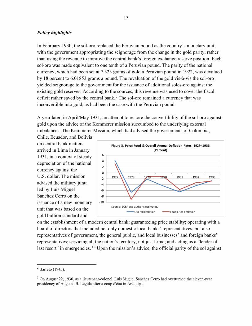
gold was further devalued by 30 percent and set at 0.421264 grams of gold per sol.5 The official parity was consistent with the then prevailing sol/U.S. dollar exchange rate of 3.6 soles per U.S. dollar. A newly established Central Reserve Bank (Banco Central de Reserva) initiated operations in 1931 with free convertibility of the sol; but because the balance of payments showed a very large deficit in 1932 that was covered by a drawdown of central bank gold reserves, the automatic effect of the convertibility was a heavy deflation (Figure 3).6 Gold exchange convertibility was therefore suspended in May 1932, and the monetary authorities moved to let the market forces freely determine the exchange rate. The sol appreciated against the U.S. dollar as the United States (under President Franklin Delano Roosevelt) abandoned the gold standard, devalued the dollar, and fixed its value at US$35 per ounce of gold in early 1933. The exchange rate oscillated freely around 4.9 soles per U.S. dollar through 1937, before gradually depreciating to 6.5 soles per dollar by mid-1940. Central bank intervention in the foreign exchange market avoided sharp fluctuations in the sol/U.S. dollar exchange rate, albeit with persistent foreign exchange sales from 1938 onwards, as war tensions developed in Europe (Barreto, 1943). The Central Reserve Bank fixed the exchange rate at 6.5 soles per U.S. dollar in June 1940, following the outbreak of the Second World War (September 1939). Fixing the exchange rate at 6.5 soles per dollar, in combination with the introduction of price controls on basic staples, manufacturing inputs and housing rents, was a de facto effort to bring about domestic price stability (Bardella, 1989, pages 291 and 352–361). Also, the war led to the introduction of exchange controls and import restrictions that forced a quick adaptation of Peru’s imports to exports throughout the period, particularly during the early years of the war. Exports to the United States were framed under temporary contracts (with the U.S. Commodity Reserve Corporation, the Rubber Reserve Company, the U.S. Defense Supply Corporation, and the Metals Reserve Company) that fixed export commodity prices and guaranteed the supply of cotton, rubber and key minerals (gold, silver, lead, zinc) to the American economy. At the same time, special trade financing arrangements, including those administered by the

4 The gold bullion standard is a system in which gold coins do not circulate, but in which the monetary authorities agree to sell gold bullion on demand at a fixed price in exchange for the circulating currency; see Banco Central de Reserva del Perú (n.d.), La Misión Kemmerer en el Perú, two volumes.

5 In contrast to the 1930 experience, the seignorage from the gold revaluation was kept with the central bank rather than transferred to the central government.

6 Balance of payments deficits reflected an array of factors in the aftermath of the 1929 Depression, including tariff hikes and trade restrictions in Peru’s export markets, a drop in world commodity prices, as well as capital outflows stemming from shortfalls in trade financing and foreign direct investment, and increased gold hoarding that triggered heavy deflation in gold-standard countries, like Peru. Increased public external debt service payments also pressured Peru’s balance of payments position. According to Barreto (1943), between January and April 1932, the Central Reserve Bank lost one third of its gold reserves which translated into a one-to-one fall in currency in circulation and heavy deflation.

15

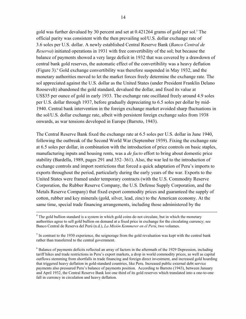
U.S. Eximbank, guaranteed the availability of inputs and machinery and equipment to Peru. During the war, official central bank reserves showed limited—but welcomed, nonetheless—increases, rising from about US$12 million (equivalent to 2.3 months of imports) in the late-1930s to about US$24 million in the mid-1940s (equivalent to 3.6 months of imports).7 The world war period was good for Peru in this regard, although the rise in official reserve coverage recorded in the early 1940s was not sustained for long (Figure 4).

The government’s decision to fix the exchange rate in June 1940 was most challenging given the underlying fiscal disequilibrium and its expansionary impact on the money supply. Indeed, in 1939–1945, Peru registered continuous fiscal deficits, largely spurred by spending overruns vis-à-vis the approved budgets (Ferrero, 1963), which led to a one-to-one increase in the national debt. Most of the national debt was central bank credit to the government, although commercial banks and the Credit and Commission Fund (Caja de Credito y Consignaciónes) also provided deficit financing through the holding/refinancing of government securities and cash advances in lieu of future tax collections accruing to the

7 During the 1940s, three-months of import coverage was possibly considered a minimum adequate level of international reserves by practitioners.

0.0

0.5

1.0

1.5

2.0

2.5

3.0

3.5

4.0

4.5

5.0

1934

1935

1936

1937

1938

1939

1940

1941

1942

1943

1944

1945

1946

1947

1948

1949

1950

1951

1952

1953

1954

1955

1956

1957

1958

1959

Figure 4. Peru: Central Bank's International Reserve Coverage , 1934−1959(Months of importss; at end-December)

Source: BCRP and author's estimates.

16

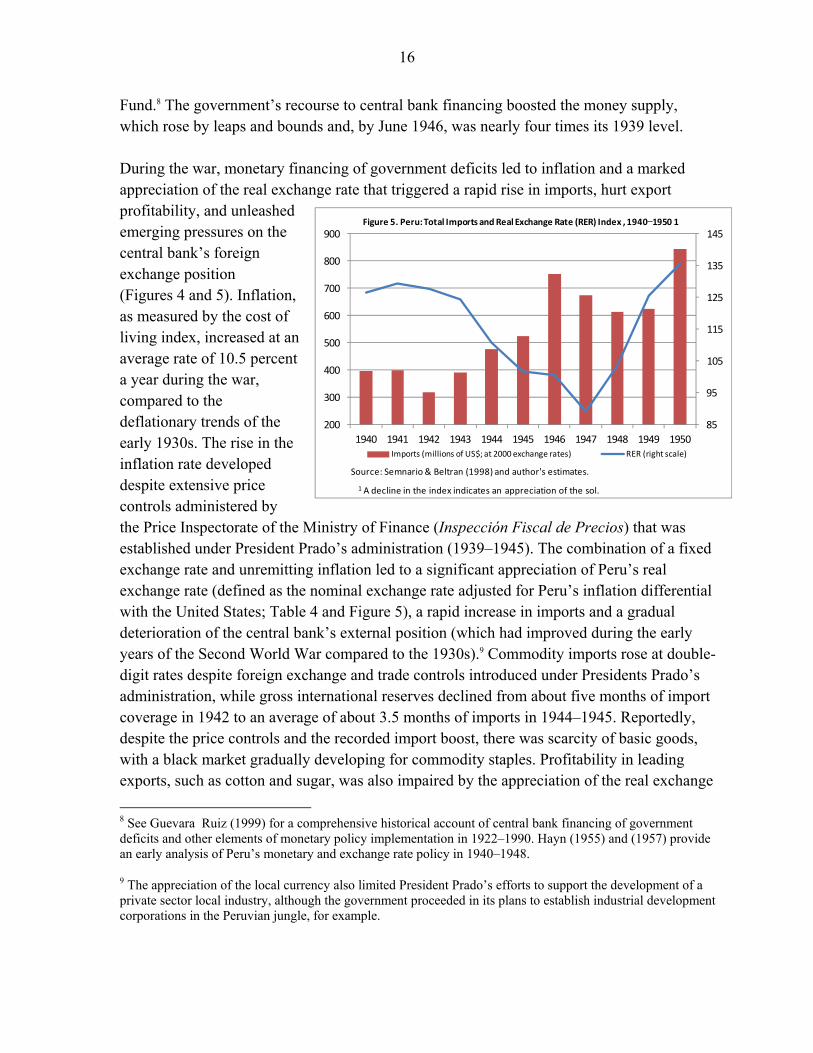
Fund.8 The government’s recourse to central bank financing boosted the money supply, which rose by leaps and bounds and, by June 1946, was nearly four times its 1939 level. During the war, monetary financing of government deficits led to inflation and a marked appreciation of the real exchange rate that triggered a rapid rise in imports, hurt export profitability, and unleashed emerging pressures on the central bank’s foreign exchange position (Figures 4 and 5). Inflation, as measured by the cost of living index, increased at an average rate of 10.5 percent a year during the war, compared to the deflationary trends of the early 1930s. The rise in the inflation rate developed despite extensive price controls administered by the Price Inspectorate of the Ministry of Finance (Inspección Fiscal de Precios) that was established under President Prado’s administration (1939–1945). The combination of a fixed exchange rate and unremitting inflation led to a significant appreciation of Peru’s real exchange rate (defined as the nominal exchange rate adjusted for Peru’s inflation differential with the United States; Table 4 and Figure 5), a rapid increase in imports and a gradual deterioration of the central bank’s external position (which had improved during the early years of the Second World War compared to the 1930s).9 Commodity imports rose at double-digit rates despite foreign exchange and trade controls introduced under Presidents Prado’s administration, while gross international reserves declined from about five months of import coverage in 1942 to an average of about 3.5 months of imports in 1944–1945. Reportedly, despite the price controls and the recorded import boost, there was scarcity of basic goods, with a black market gradually developing for commodity staples. Profitability in leading exports, such as cotton and sugar, was also impaired by the appreciation of the real exchange

8 See Guevara Ruiz (1999) for a comprehensive historical account of central bank financing of government deficits and other elements of monetary policy implementation in 1922–1990. Hayn (1955) and (1957) provide an early analysis of Peru’s monetary and exchange rate policy in 1940–1948.

9 The appreciation of the local currency also limited President Prado’s efforts to support the development of a private sector local industry, although the government proceeded in its plans to establish industrial development corporations in the Peruvian jungle, for example.

85

95

105

115

125

135

145

200

300

400

500

600

700

800

900

1940 1941 1942 1943 1944 1945 1946 1947 1948 1949 1950

Figure 5. Peru: Total Imports and Real Exchange Rate (RER) Index , 1940−1950 1

Imports (millions of US$; at 2000 exchange rates) RER (right scale)

Source: Semnario & Beltran (1998) and author's estimates.

1 A decline in the index indicates an appreciation of the sol.

17

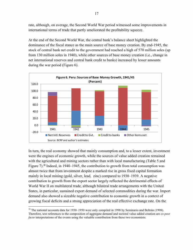
rate, although, on average, the Second World War period witnessed some improvements in international terms of trade that partly ameliorated the profitability squeeze. At the end of the Second World War, the central bank’s balance sheet highlighted the dominance of the fiscal stance as the main source of base money creation. By end-1945, the stock of central bank net credit to the government had reached a high of 570 million soles (up from 130 million soles in 1940), while other sources of base money creation (i.e., change in net international reserves and central bank credit to banks) increased by lesser amounts during the war period (Figure 6).

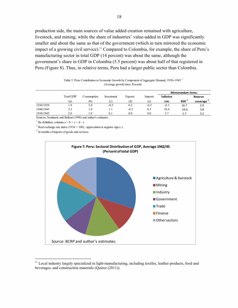
In turn, the real economy showed that mainly consumption and, to a lesser extent, investment were the engines of economic growth, while the sources of value added creation remained with the agricultural and mining sectors rather than with local manufacturing (Table 5 and Figure 7).10 Indeed, in 1940–1945, the contribution to growth from total consumption was almost twice that from investment despite a marked rise in gross fixed capital formation mainly in local mining (gold, silver, lead, zinc) compared to 1930–1939. A negative contribution to growth from the export sector largely reflected the detrimental effects of World War II on multilateral trade, although bilateral trade arrangements with the United States, in particular, sustained export demand of selected commodities during the war. Import demand also showed a sizeable negative contribution to economic growth in a context of growing fiscal deficits and a strong appreciation of the real effective exchange rate. On the 10 The national accounts data for 1930–1950 were only compiled in 1998 by Seminario and Beltrán (1998). Therefore, text references to the composition of aggregate demand and sectoral value added creation are ex-post facto interpretations of the events using the valuable contribution from these two economists.

-20.0

0.0

20.0

40.0

60.0

80.0

100.0

120.0

1941 1942 1943 1944 1945

Figure 6. Peru: Sources of Base Money Growth, 1941/45 (Percent)

Net Intl. Reserves Credit to Gvt. Credit to banks Other items net

Source: BCRP and author's estimates.

18

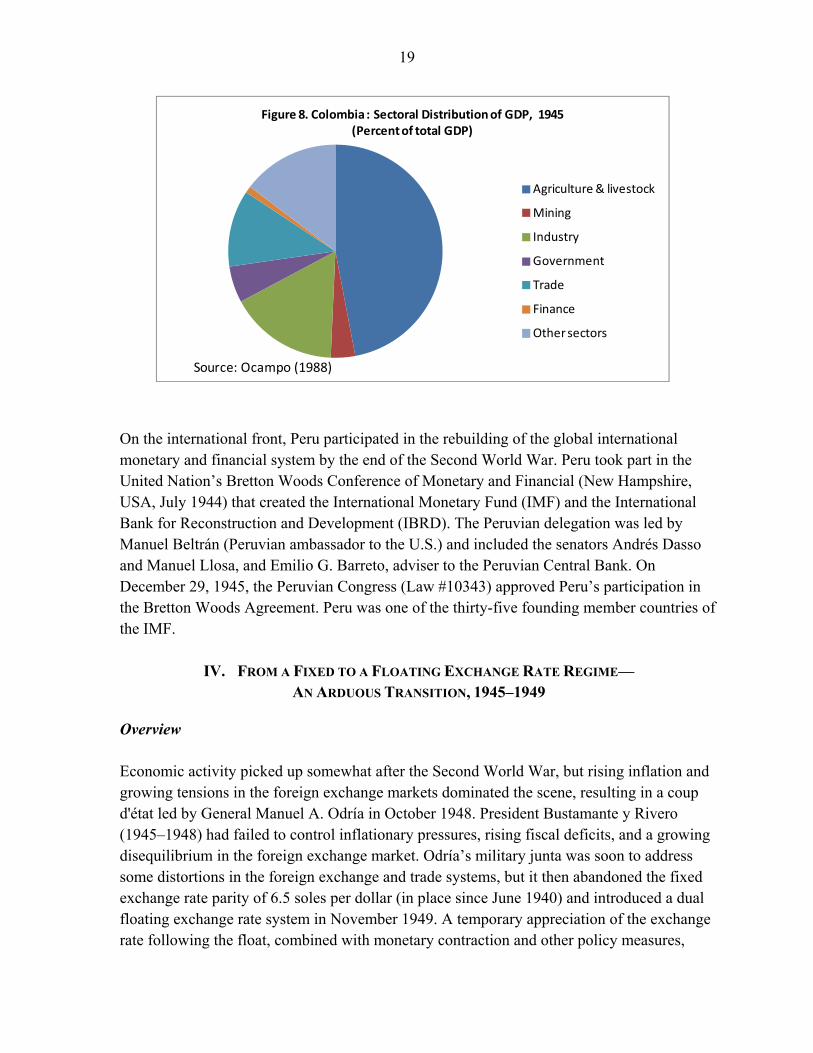
production side, the main sources of value added creation remained with agriculture, livestock, and mining, while the share of industries’ value-added in GDP was significantly smaller and about the same as that of the government (which in turn mirrored the economic impact of a growing civil service).11 Compared to Colombia, for example, the share of Peru’s manufacturing sector in total GDP (14 percent) was about the same, although the government’s share in GDP in Colombia (5.5 percent) was about half of that registered in Peru (Figure 8). Thus, in relative terms, Peru had a larger public sector than Colombia.

11 Local industry largely specialized in light-manufacturing, including textiles, leather products, food and beverages, and construction materials (Quiroz (2011)).

Total GDP Consumption Investment Exports Imports Inflation Reserve

(a) (b) (c) (d) (e) rate RER 2 coverage 3

1930/1939 1.9 2.0 -0.5 0.2 -0.2 -0.3 16.7 2.9

1940/1945 2.3 1.9 1.1 -0.3 0.3 10.4 -19.6 3.8

1930/1945 2.0 1.9 0.1 0.0 0.0 3.7 1.7 3.2

Sources: Seminario and Beltran (1998) and author's estimates.1 By definition, columns a = b + c + d - e2 Real exchange rate index (1934 = 100) ; appreciation is negative sign (-).3 In months of imports of goods and services.

Table 5. Peru: Contribution to Economic Growth by Component of Aggregate Demand, 1930–1945 1

(Average growth rates; Percent)

Memorandum items:

Figure 7: Peru: Sectoral Distribution of GDP, Average 1942/45 (Percent of total GDP)

Agriculture & livestock

Mining

Industry

Government

Trade

Finance

Other sectors

Source: BCRP and author's estimates.

19

On the international front, Peru participated in the rebuilding of the global international monetary and financial system by the end of the Second World War. Peru took part in the United Nation’s Bretton Woods Conference of Monetary and Financial (New Hampshire, USA, July 1944) that created the International Monetary Fund (IMF) and the International Bank for Reconstruction and Development (IBRD). The Peruvian delegation was led by Manuel Beltrán (Peruvian ambassador to the U.S.) and included the senators Andrés Dasso and Manuel Llosa, and Emilio G. Barreto, adviser to the Peruvian Central Bank. On December 29, 1945, the Peruvian Congress (Law #10343) approved Peru’s participation in the Bretton Woods Agreement. Peru was one of the thirty-five founding member countries of the IMF.

IV. FROM A FIXED TO A FLOATING EXCHANGE RATE REGIME— AN ARDUOUS TRANSITION, 1945–1949

Overview Economic activity picked up somewhat after the Second World War, but rising inflation and growing tensions in the foreign exchange markets dominated the scene, resulting in a coup d'état led by General Manuel A. Odría in October 1948. President Bustamante y Rivero (1945–1948) had failed to control inflationary pressures, rising fiscal deficits, and a growing disequilibrium in the foreign exchange market. Odría’s military junta was soon to address some distortions in the foreign exchange and trade systems, but it then abandoned the fixed exchange rate parity of 6.5 soles per dollar (in place since June 1940) and introduced a dual floating exchange rate system in November 1949. A temporary appreciation of the exchange rate following the float, combined with monetary contraction and other policy measures,

Figure 8. Colombia : Sectoral Distribution of GDP, 1945 (Percent of total GDP)

Agriculture & livestock

Mining

Industry

Government

Trade

Finance

Other sectors

Source: Ocampo (1988)

20

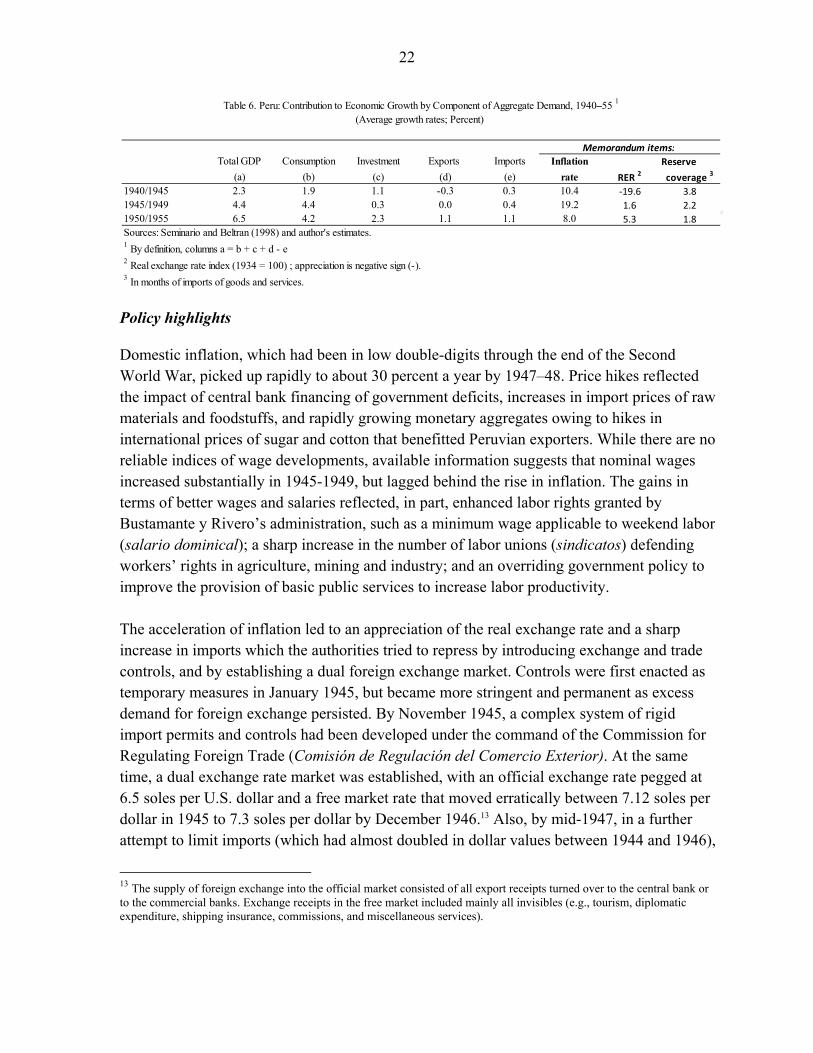
brought down inflation significantly by end-1949. The first mission from the IMF had arrived in Lima in February 1947 and began a process of technical consultations with the government that were to become a practice through the following 30 years (Box 1).12 The economic challenges faced by President Bustamante y Rivero were massive. The national accounts indicate that economic growth reflected the growth in consumption rather than in productive investment and/or exports (Table 6). The contribution of total consumption to economic growth far surpassed the combined contribution of investment and exports, as the investment/export-led recovery during the Second World War had faded away. Another constant between 1945–49 and 1940–45 was the negative contribution of imports on economic growth in a context of large fiscal deficits and recurrent foreign exchange market pressures that the government tried in vain to address through exchange and trade controls. A rising population growth rate, combined with large migration from the rural areas into the urban centers, gave rise to the need for an alternative, export-oriented, investment-led, growth model which was initiated under the military junta led by General Odría.

12 The IMF mission included IMF Acting Managing Director, Harry Dexter White; the IMF Executive Director representing Peru, Francisco dos Santos; economists Robert Triffin; and A. Thaokara. Harry Dexter White had been the senior U.S. government official who, together with John Maynard Keynes, dominated the July 1944 Bretton Woods Conference that created the IMF and the IBRD. See, EB Document No. 130, Initial Par Values —Peru, 11/25/1946, IMF Archives; Staff Memo No. 43, Exchange Market in Peru, 1/29/1947, IMF Archives.

21

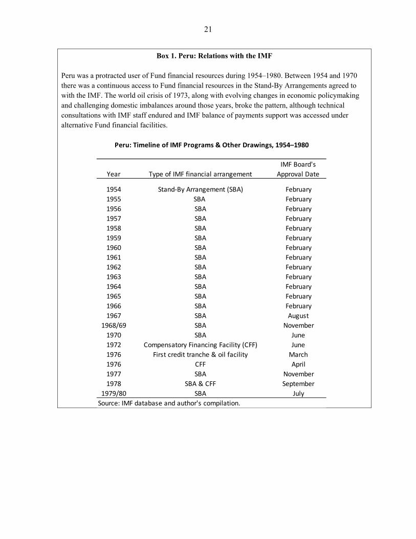
Box 1. Peru: Relations with the IMF Peru was a protracted user of Fund financial resources during 1954–1980. Between 1954 and 1970 there was a continuous access to Fund financial resources in the Stand-By Arrangements agreed to with the IMF. The world oil crisis of 1973, along with evolving changes in economic policymaking and challenging domestic imbalances around those years, broke the pattern, although technical consultations with IMF staff endured and IMF balance of payments support was accessed under alternative Fund financial facilities.

Year Type of IMF financial arrangement

IMF Board's

Approval Date

1954 Stand-By Arrangement (SBA) February

1955 SBA February

1956 SBA February

1957 SBA February

1958 SBA February

1959 SBA February

1960 SBA February

1961 SBA February

1962 SBA February

1963 SBA February

1964 SBA February

1965 SBA February

1966 SBA February

1967 SBA August

1968/69 SBA November

1970 SBA June

1972 Compensatory Financing Facility (CFF) June

1976 First credit tranche & oil facility March

1976 CFF April

1977 SBA November

1978 SBA & CFF September

1979/80 SBA July

Source: IMF database and author's compilation.

Peru: Timeline of IMF Programs & Other Drawings, 1954–1980

22

Policy highlights

Domestic inflation, which had been in low double-digits through the end of the Second World War, picked up rapidly to about 30 percent a year by 1947–48. Price hikes reflected the impact of central bank financing of government deficits, increases in import prices of raw materials and foodstuffs, and rapidly growing monetary aggregates owing to hikes in international prices of sugar and cotton that benefitted Peruvian exporters. While there are no reliable indices of wage developments, available information suggests that nominal wages increased substantially in 1945-1949, but lagged behind the rise in inflation. The gains in terms of better wages and salaries reflected, in part, enhanced labor rights granted by Bustamante y Rivero’s administration, such as a minimum wage applicable to weekend labor (salario dominical); a sharp increase in the number of labor unions (sindicatos) defending workers’ rights in agriculture, mining and industry; and an overriding government policy to improve the provision of basic public services to increase labor productivity. The acceleration of inflation led to an appreciation of the real exchange rate and a sharp increase in imports which the authorities tried to repress by introducing exchange and trade controls, and by establishing a dual foreign exchange market. Controls were first enacted as temporary measures in January 1945, but became more stringent and permanent as excess demand for foreign exchange persisted. By November 1945, a complex system of rigid import permits and controls had been developed under the command of the Commission for Regulating Foreign Trade (Comisión de Regulación del Comercio Exterior). At the same time, a dual exchange rate market was established, with an official exchange rate pegged at 6.5 soles per U.S. dollar and a free market rate that moved erratically between 7.12 soles per dollar in 1945 to 7.3 soles per dollar by December 1946.13 Also, by mid-1947, in a further attempt to limit imports (which had almost doubled in dollar values between 1944 and 1946),

13 The supply of foreign exchange into the official market consisted of all export receipts turned over to the central bank or to the commercial banks. Exchange receipts in the free market included mainly all invisibles (e.g., tourism, diplomatic expenditure, shipping insurance, commissions, and miscellaneous services).

Total GDP Consumption Investment Exports Imports Inflation Reserve

(a) (b) (c) (d) (e) rate RER 2 coverage 3

1940/1945 2.3 1.9 1.1 -0.3 0.3 10.4 -19.6 3.8

1945/1949 4.4 4.4 0.3 0.0 0.4 19.2 1.6 2.2

1950/1955 6.5 4.2 2.3 1.1 1.1 8.0 5.3 1.8

Sources: Seminario and Beltran (1998) and author's estimates.1 By definition, columns a = b + c + d - e2 Real exchange rate index (1934 = 100) ; appreciation is negative sign (-).3 In months of imports of goods and services.

Memorandum items:

(Average growth rates; Percent) Table 6. Peru: Contribution to Economic Growth by Component of Aggregate Demand, 1940–55 1

23

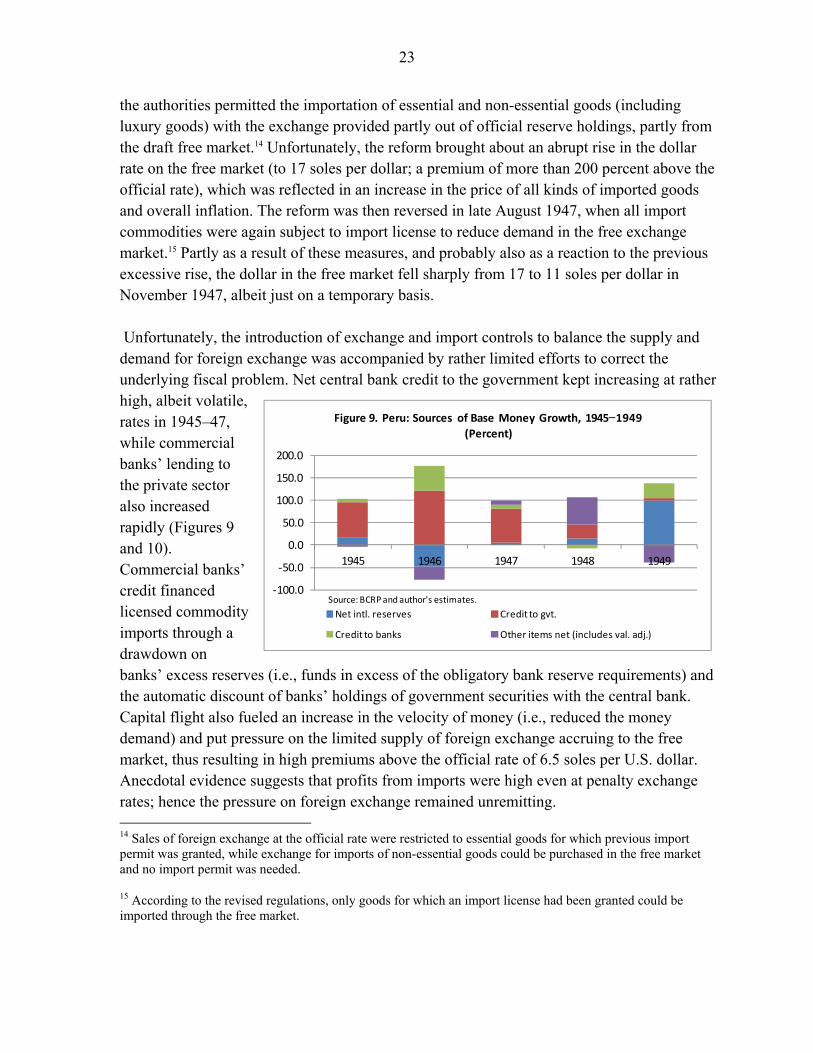
the authorities permitted the importation of essential and non-essential goods (including luxury goods) with the exchange provided partly out of official reserve holdings, partly from the draft free market.14 Unfortunately, the reform brought about an abrupt rise in the dollar rate on the free market (to 17 soles per dollar; a premium of more than 200 percent above the official rate), which was reflected in an increase in the price of all kinds of imported goods and overall inflation. The reform was then reversed in late August 1947, when all import commodities were again subject to import license to reduce demand in the free exchange market.15 Partly as a result of these measures, and probably also as a reaction to the previous excessive rise, the dollar in the free market fell sharply from 17 to 11 soles per dollar in November 1947, albeit just on a temporary basis. Unfortunately, the introduction of exchange and import controls to balance the supply and demand for foreign exchange was accompanied by rather limited efforts to correct the underlying fiscal problem. Net central bank credit to the government kept increasing at rather high, albeit volatile, rates in 1945–47, while commercial banks’ lending to the private sector also increased rapidly (Figures 9 and 10). Commercial banks’ credit financed licensed commodity imports through a drawdown on banks’ excess reserves (i.e., funds in excess of the obligatory bank reserve requirements) and the automatic discount of banks’ holdings of government securities with the central bank. Capital flight also fueled an increase in the velocity of money (i.e., reduced the money demand) and put pressure on the limited supply of foreign exchange accruing to the free market, thus resulting in high premiums above the official rate of 6.5 soles per U.S. dollar. Anecdotal evidence suggests that profits from imports were high even at penalty exchange rates; hence the pressure on foreign exchange remained unremitting. 14 Sales of foreign exchange at the official rate were restricted to essential goods for which previous import permit was granted, while exchange for imports of non-essential goods could be purchased in the free market and no import permit was needed.

15 According to the revised regulations, only goods for which an import license had been granted could be imported through the free market.

-100.0

-50.0

0.0

50.0

100.0

150.0

200.0

1945 1946 1947 1948 1949

Figure 9. Peru: Sources of Base Money Growth, 1945−1949

(Percent)

Net intl. reserves Credit to gvt.

Credit to banks Other items net (includes val. adj.)

Source: BCRP and author's estimates.

24

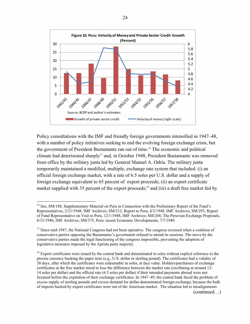
Policy consultations with the IMF and friendly foreign governments intensified in 1947–48, with a number of policy initiatives seeking to end the evolving foreign exchange crisis, but the government of President Bustamante ran out of time.16 The economic and political climate had deteriorated sharply17 and, in October 1948, President Bustamante was removed from office by the military junta led by General Manuel A. Odría. The military junta temporarily maintained a modified, multiple, exchange rate system that included: (i) an official foreign exchange market, with a rate of 6.5 soles per U.S. dollar and a supply of foreign exchange equivalent to 65 percent of export proceeds; (ii) an export certificate market supplied with 35 percent of the export proceeds;18 and (iii) a draft free market fed by

16 See, SM/188, Supplementary Material on Peru in Connection with the Preliminary Report of the Fund’s Representatives, 2/21/1948, IMF Archives; SM/212, Report to Peru, 4/2/1948, IMF Archives; SM/293, Report of Fund Representative on Visit to Peru, 12/1/1948, IMF Archives; SM/268, The Peruvian Exchange Proposals, 8/31/1948, IMF Archives; SM/375, Peru: recent Economic Developments, 7/7/1949.

17 Since mid-1947, the National Congress had not been operative. The congress recessed when a coalition of conservative parties opposing the Bustamante’s government refused to attend its sessions. The move by the conservative parties made the legal functioning of the congress impossible, preventing the adoption of legislative measures imposed by the Aprista party majority.

18 Export certificates were issued by the central bank and denominated in soles without explicit reference to the precise currency backing the paper note (e.g., U.S. dollar or sterling pound). The certificates had a validity of 30 days, after which the certificates were redeemable in soles, at face value. Holders/purchasers of exchange certificates in the free market stood to lose the difference between the market rate (oscillating at around 12–14 soles per dollar) and the official rate (6.5 soles per dollar) if their intended payments abroad were not licensed before the expiration of their exchange certificates. In 1947–49, the central bank faced the problem of excess supply of sterling pounds and excess demand for dollar-denominated foreign exchange, because the bulk of imports backed by export certificates were out of the American market. The situation led to misalignments

(continued…)

44.24.44.64.855.25.45.65.86

0

5

10

15

20

25

30

Figure 10. Peru: Velocity of Money and Private Sector Credit Growth

(Percent)

Growth of private sector credit Velocity of money (right scale)

Source: BCRP and author's estimates.

25

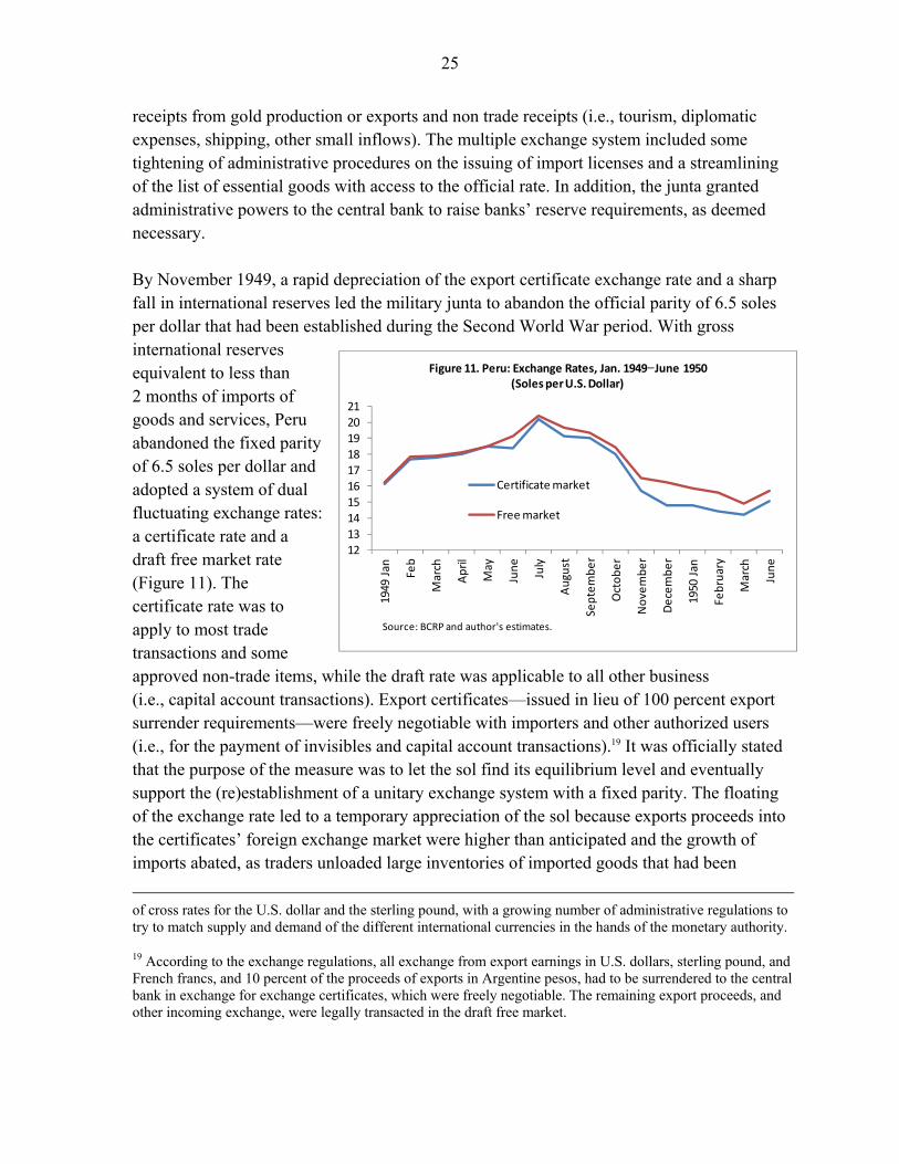
receipts from gold production or exports and non trade receipts (i.e., tourism, diplomatic expenses, shipping, other small inflows). The multiple exchange system included some tightening of administrative procedures on the issuing of import licenses and a streamlining of the list of essential goods with access to the official rate. In addition, the junta granted administrative powers to the central bank to raise banks’ reserve requirements, as deemed necessary. By November 1949, a rapid depreciation of the export certificate exchange rate and a sharp fall in international reserves led the military junta to abandon the official parity of 6.5 soles per dollar that had been established during the Second World War period. With gross international reserves equivalent to less than 2 months of imports of goods and services, Peru abandoned the fixed parity of 6.5 soles per dollar and adopted a system of dual fluctuating exchange rates: a certificate rate and a draft free market rate (Figure 11). The certificate rate was to apply to most trade transactions and some approved non-trade items, while the draft rate was applicable to all other business (i.e., capital account transactions). Export certificates—issued in lieu of 100 percent export surrender requirements—were freely negotiable with importers and other authorized users (i.e., for the payment of invisibles and capital account transactions).19 It was officially stated that the purpose of the measure was to let the sol find its equilibrium level and eventually support the (re)establishment of a unitary exchange system with a fixed parity. The floating of the exchange rate led to a temporary appreciation of the sol because exports proceeds into the certificates’ foreign exchange market were higher than anticipated and the growth of imports abated, as traders unloaded large inventories of imported goods that had been

of cross rates for the U.S. dollar and the sterling pound, with a growing number of administrative regulations to try to match supply and demand of the different international currencies in the hands of the monetary authority.

19 According to the exchange regulations, all exchange from export earnings in U.S. dollars, sterling pound, and French francs, and 10 percent of the proceeds of exports in Argentine pesos, had to be surrendered to the central bank in exchange for exchange certificates, which were freely negotiable. The remaining export proceeds, and other incoming exchange, were legally transacted in the draft free market.

12131415161718192021

1949

Jan Fe

b

Mar

ch

Ap

ril

May

Jun

e

July

Au

gust

Sep

tem

be

r

Oct

ob

er

No

vem

be

r

De

cem

be

r

1950

Jan

Feb

ruar

y

Mar

ch

Jun

e

Figure 11. Peru: Exchange Rates, Jan. 1949−June 1950 (Soles per U.S. Dollar)

Certificate market

Free market

Source: BCRP and author's estimates.

26

accumulated because of fears of further exchange depreciation. There was also a lengthening of the maturity of exchange certificates (from 30 to 60 days to increase the float) that reduced exchange rate pressures. In addition, the central bank invigorated its efforts to check banks’ excessive credit expansion to the private sector through the establishment of credit ceilings per individual bank borrower and increases in banks’ reserve requirements to tighten the growth of broad money. The liberalization in the exchange system of November 1949 was highly influenced by the Klein Mission Report.20 The report, which had been prepared by technicians contracted in the United States to advise the Peruvian government on economic and financial matters, supported the preparation of the Decree-Law No. 11208 that abandoned the official parity of the sol and authorized exporters to receive exchange certificates for the full amount of the value of their exports. The report argued that the central bank should not intervene in the foreign exchange market, while noting that the achievement of a “normal and continuing” exchange rate in the free market may take some time. The report expected a temporary appreciation of the rate (as actually happened) owing to the increased supply of dollars into the exchange market which would diminish eventually owing to export seasonality factors. Also, the Klein Mission Report emphasized the need to make Peru a desirable destination of U.S. FDI by fostering a profitable export sector through a competitive exchange rate. The latter was viewed to benefit the depressed traditional (e.g., sugar, cotton, copper and petroleum) and nontraditional exports (coal, cement, fish, textiles); a most palatable and timely idea for the government of President Odría. President Odría’s administration was quick to support an increase in FDI along the lines of the exchange market liberalization recommended by the Klein Mission Report. A number of legal measures to stimulate the mining industry were adopted during those years. In August 1949, two months before the exchange reform, the mining industry received permission to sell all its exchange at the certificate rate. A new mining code was promulgated in May 1950. It exempted mining concerns for a period of 25 years from all export taxes existing or to be introduced in the future, except the income tax and certain land taxes. Several sizeable investment projects took off following the implementation of the new mining code: a new zinc refinery operated by the Cerro de Pasco Corporation; new explorations of rich copper deposits in Southern Peru (Toquepala and Quellaveco) by the U.S. subsidiary Peru Mining and Smelting Company. Manganese and tungsten production, financed by the Peruvian Mining Bank and loans from the U.S. Eximbank, was also increased. Finally, in July 1951, a contract was signed between French financial interests and the government-owned Peruvian

20 See, Julius Klein (1949) and S. C. Tsiang (1956).

27

Santa Rosa Corporation for the erection of an iron and steel plant at the Port of Chimbote. A new oil code was introduced by the government to the congress in August 1950.

V. POLICY CHALLENGES DURING PRESIDENT ODRÍA’S ECONOMIC BONANZA AND

AFTERWARD, 1950–1959

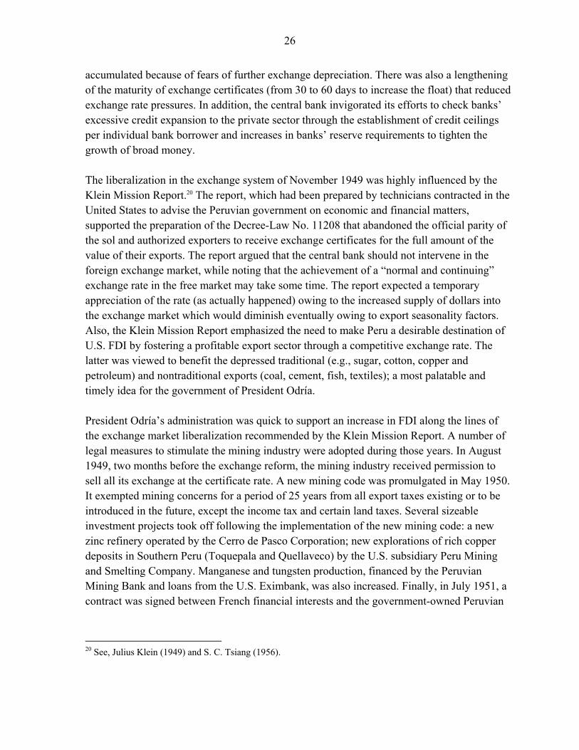
Overview Investment-to-GDP ratios reached a historical peak in the 1950s, while Peru became a net borrower of external savings to finance its investment program (Figure 12). Large public investment projects in basic infrastructure and social sectors, combined with FDI in the export-led mining centers of Cerro de Pasco, Toquepala, Quellaveco, Marcona, and others delivered high rates of economic growth. Also, a rising, labor-intensive fishmeal industry, with a number of intersectoral linkages with local industry, was an important source of private sector investment, employment, and foreign exchange receipts.21 The high investment ratios (averaging 25 percent of GDP during most of the decade) were financed by large external current account deficits (of about 3 percent of GDP) that supplied foreign savings to the economy (mainly as FDI inflows) and by domestic private and public sector savings (totaling some 22 percent of GDP). The recording of positive government savings during the 1950s was a unique situation for an economy traditionally characterized by large fiscal deficits. During the 1950s, macroeconomic trends were marked by growing, albeit volatile, export receipts; a situation that reinforced the authorities’ decision to retain a floating exchange rate

21 See, for example, Gertrud Lovasy (1961) and Michael Roemer (1970).

-5.0

0.0

5.0

10.0

15.0

20.0

25.0

30.0

1930/1939 1940/1945 1945/1949 1950/1955 1956/1959

Figure 12. Peru: Savings - Investment Balance (Percent of GDP)

External current account (surplus, -) Public savings Private savings Investment

Source: BCRP and author's estimates.

28

system despite the prevailing Bretton Woods system of fixed exchange rates (Box 2). Export values and volumes rose with rapid export diversification: minerals (copper, zinc, nickel) registered growing shares in export totals, as did coffee and fishmeal, while cotton and sugar shares declined. Marked slowdowns in export receipts did happen, however, at the end of the Korean War (1953) and in 1957–1959, when Peru’s international terms of trade experienced an important deterioration. In the 1950–1959, Peru retained its dual floating exchange rate system which was introduced in November 1949, with the rates in the certificates and draft free markets generally depreciating in line with domestic inflation and moving within a narrow spread.22 The government’s view was that the system of floating rates ensured the repatriation of export proceeds and the availability of funds to handle current and capital account transactions. Also, the authorities argued that, despite the progress achieved in terms of price and exchange rate stability in the 1950s, the instability in the international markets for Peru’s main exports and the relatively low level of central bank gross international reserves, remained obstacles for setting a new exchange rate parity, without re-establishing exchange and trade controls. Thus, the government’s decision to maintain a dual system of floating exchange rates contrasted with the then prevailing paradigm of fixed parities under the Bretton Woods system (Box 2). Another feature of this period was that President Odría (1948–1956) and President Prado (1956–1962) worked with the international financial community in addressing the macroeconomic challenges of their times. Under President Odría, the U.S. Government, the Chase Manhattan Bank of New York and the IMF supported the government’s efforts to control inflation and stabilize the exchange rate. The background was one of rapidly growing credit and monetary aggregates along with a brisk pace of economic activity, and booming FDI. In turn, President Prado governed in a period of decelerating export receipts, dwindling FDI, and enduring fiscal deficits that were addressed only in mid-1959. Like his predecessor, President Prado sought support from the international financial community to address Peru’s internal and external imbalances.

22 See, Executive Board Meeting (EBM) 626, Par Value-Peru, 12/18/1950, IMF Archives and EBM/52/69, 1952 Consultations-Peru, IMF Archives.

29

Box 2. The Bretton Woods System

The Bretton Woods system of monetary management established the rules for commercial and financial relations among the world's major industrial states in the mid-twentieth century. The system was the first example of a fully negotiated monetary order intended to govern monetary relations among independent nation-states. The chief features of the Bretton Woods system were an obligation for each country to establish a parity of their national currencies in terms of the reserve currency (a "peg") and to maintain exchange rates within plus or minus 1 percent of parity (a "band") by intervening in their foreign exchange markets (that is, buying or selling foreign money). Member countries could only change their par value with IMF approval, which was contingent on IMF determination that a country’s balance of payments was in a "fundamental disequilibrium." In theory, the reserve currency would be the bancor (a world currency unit that was never implemented), suggested by John Maynard Keynes at the Bretton Woods conference (July 1944); but the United States objected and their request was granted, making the "reserve currency" the U.S. dollar. Thus, the U.S. dollar took over the role that gold had played under the gold standard in the international financial system. Meanwhile, to bolster faith in the dollar, the U.S. agreed separately to link the dollar to gold at the rate of US$35 per ounce of gold. At this rate, foreign governments and central banks were able to exchange dollars for gold. On August 15, 1971, the United States unilaterally terminated convertibility of the dollar to gold. As a result, the Bretton Woods system officially ended and the dollar became fully “fiat currency,” backed by nothing but the promise of the U.S. federal government. By 1973, most major world economies had allowed their currencies to float freely against the dollar. An economic paradox of Odría’s economic bonanza during the early-1950s was that the observed balance of payments surpluses and income growth did not translate into solid improvements in the central bank’s international reserve position. The Polak model (Box 3), which was the basic analytical framework of IMF missions around the world, provided explanations for these apparently counterintuitive results and thus became a common technical language between Peruvian policymakers and the IMF staff through decades of engagement. The model, which was based on the idea that the balance of payments is essentially a monetary phenomenon, emphasized the linkages between the stance of credit policies and their inverse relationship with the country’s international reserves position.

30

Box 3. The Polak Model

In the 1950s, Jacques J. Polak and his colleagues in the IMF Research department developed an economic model reflecting the monetary approach to the balance of payments.23 The model sought to integrate monetary, income, and balance of payments analysis, and it became the basis for conditionality applied to IMF credits to member countries. Extremely simple, with a primary focus on balance of payments effects of credit expansion by the banking system, the model has retained its usefulness for policy purposes over time and, to date, it is still being adapted to changes in countries’ priorities and in the international monetary system. Polak’s analysis took as its point of departure the empirical fact that in some countries money and income expansion were positively related, while in others the relationship was negative. Polak and his colleagues illustrated how a monetary approach could provide analytical support for the proposition that an expansion of income would be accompanied by a fall in the money supply. The basic reasoning was that higher incomes will lead to higher imports (and exports will also tend to decline as more resources are absorbed internally). The balance of payments will go into deficit, and the fall in the stock of international reserves will lead to a decline in the money supply. In guiding the IMF’s operational work, Polak emphasized that to integrate monetary analysis into income analysis, domestic credit had to be the policy, or control, variable. Polak’s theoretical and quantitative analysis showed that, in the long run, a temporary expansion in domestic credit is matched by a loss of international reserves. This one-for-one relationship between changes in domestic credit and international reserves was the fundamental equation of the monetary approach to the balance of payments. To use the Polak model to formulate policy, one simply need choose a target value for the endogenous variable, say the level of international reserves; calculate the value of the exogenous variables in the system (exports and capital flows); and then solve for the expansion of domestic credit that would be consistent with the target.

Policy highlights As noted, the period’s initial conditions were rather good, with Peru profiting from a favorable environment on the domestic and the international front. On the domestic front, the sol had strengthened and inflation had come down following the exchange rate liberalization of November 1949, while output growth and investment expectations were up along with an

23 Robert Triffin, who was a member of the first IMF mission to Peru in February 1947, was Jacques Polak’s colleague at the IMF Research department and a leading intellectual figure in the development of the monetary approach in the IMF (Triffin, 1946).

31

optimistic outlook for private sector development.24 At the same time, the budget deficit was being brought under control and the growth of commercial bank credit had decelerated owing to increases in banks’ average and marginal reserve requirements and the setting of credit ceilings on individual bank borrowers. On the external front, the government’s warm support of FDI translated into important capital inflows that financed a rising current account imbalance. Also, between 1952 and 1954, the government reached agreement with external creditors on the servicing of Peruvian bonds that had been in default since 1931. The outbreak of the Korean War benefitted Peruvian exports, which experienced important increases in international commodity prices, especially for metals. In 1950–1951, the inflationary effect of rising capital inflows and monetary aggregates challenged Peruvian policymakers, who stood up to the challenge and delivered price and exchange rate stability. In September 1951, the banking superintendency introduced a number of deflationary policies to arrest the growth of monetary and credit aggregates. The superintendency increased banks’ average and marginal reserve requirements; enacted selective controls on commercial banks’ import trade credit;25 curtailed the banks’ prerogative to automatically discount treasury bills with the central bank; and put limits on banks’ lending for real estate, residential construction, and the financing of consumer durables. At the same time, surrender requirements on export proceeds were lowered to induce an increase of private sector holdings of foreign assets abroad. All in all, by end-1951, the growth of monetary and credit aggregates had slowed down, the annual inflation rate had stabilized below 10 percent, and both the certificate and the draft free market exchange rates stood at 15.2 soles per U.S. dollar, compared with 15.4 soles per dollar at end-December 1950.26 Gross international reserves rose from US$36 million at end-1950 to US$45 million at end-1951 (equivalent to 1.9 months of goods and services imports).27 By end-1952, gross reserves remained at around US$45 million, while the certificate and the draft free market exchange rates averaged 15.6 soles per U.S. dollar.

24 Optimism over President Odría’s government policies was summarized by press reports in the international press. See, Irving Kalin (1953).

25 Effective February 1, 1951, all import prohibitions had been eliminated. Partly as a result of this policy and partly because of anticipatory buying after the start of the Korean War, Peruvian imports reached an all-time high of US$260 million in 1951, compared with US$175 million in 1950.

26 In1949-1953, the spreads between the certificate exchange rate and the rate in the free market were less than 1 percent, on average.

27 The referred levels of gross international reserves excluded US$18.4 million of “untouchable” gold reserves valued at US$35 per ounce.

32

In 1953, the sol again came under pressure because of a deterioration of the international terms of trade in the aftermath of the Korean conflict. The exchange rate in the certificate and the draft free market increased to 19.43 soles per dollar in late-December 1953. Export proceeds from sugar, cotton, and main minerals suffered from a drop in the international commodity prices, while imports rose partly as a result of increased FDI (that boosted imports of machinery and equipment) and partly on account of hikes in durable and non-durable commodity imports following the elimination of all import prohibitions in February 1951. The policy response to the exchange rate pressures was again swift, including strong deflationary fiscal and monetary measures, as Peru agreed to its first Stand-By Arrangement with the IMF in February 1954.28 Peru was the first Latin American country to sign a Stand-By Arrangement with the IMF. The financial arrangement was approved by the IMF Executive Board on February 17, 1954 and it was followed by a public address to the nation by President Odría (Box 4). The Stand-By Arrangement with Peru was the first one extended by the IMF to a country without a par value against the U.S. dollar. By February 1954, the only other country in the world with floating exchange rates and negligible exchange and trade restrictions was Canada. Peru and Canada were reportedly enjoying the highest rates of foreign private investment in the world. Performance under the 1954 economic program was remarkably successful. Inflation dropped to 5.5 percent, the velocity of circulation of money declined (money demand increased), and the exchange rate stabilized at around 19 soles per U.S. dollar, while economic growth continued at a brisk pace, supported by sizeable exports and investment spending.29 The overall balance of payments registered a small surplus that permitted some marginal increase in gross international reserves. Peru did not draw on any of the lines of credit provided by the IMF, the U.S. Treasury, or the Chase Manhattan Bank of New York. The thrust of the financial stabilization program implemented by the Odría administration was consistent with the monetary approach to the balance of payments predicated under the Polak model. The control variable under the program was domestic credit, while the target variable was the country’s international reserve position. The implementation of deflationary policies under the 1954 and subsequent IMF-supported programs during the Odría administration reduced the contribution of total consumption to economic growth, while 28 See, EBM/54/6, Use of Fund’s Resources – Peru, 2/12/1954; EBM/54/7, 1953 Consultations and Use of the Fund’s Resources – Peru, 2/17/1954, IMF Archives.

29 According to the records, chief policymakers of that time included Messrs. A. F. Dasso, President of the Central Reserve Bank of Peru (BCRP), E. Guimoye, Minister of Finance, F. R. Huidobro, Superintendent of Banks, and E.G. Barreto, Chief of the Office of Economic Studies of the BCRP.

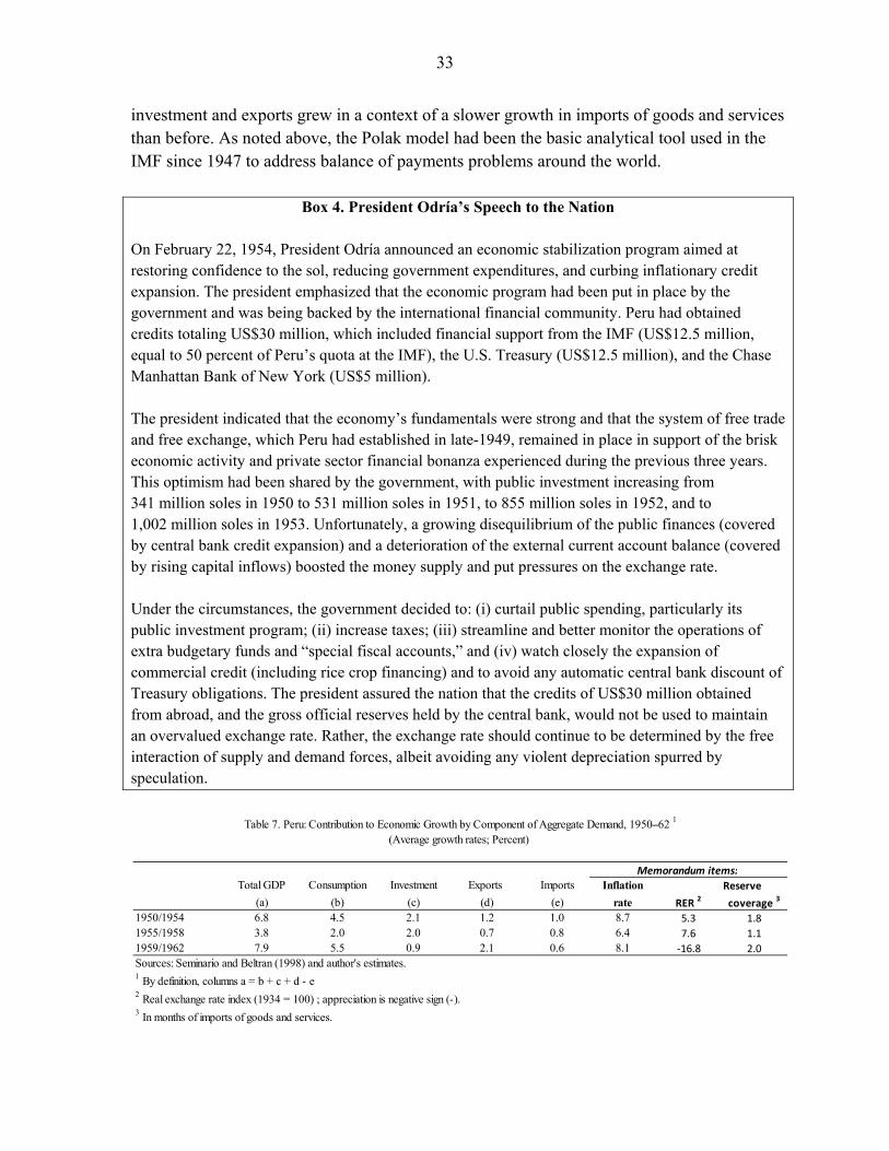
33

investment and exports grew in a context of a slower growth in imports of goods and services than before. As noted above, the Polak model had been the basic analytical tool used in the IMF since 1947 to address balance of payments problems around the world.

Box 4. President Odría’s Speech to the Nation On February 22, 1954, President Odría announced an economic stabilization program aimed at restoring confidence to the sol, reducing government expenditures, and curbing inflationary credit expansion. The president emphasized that the economic program had been put in place by the government and was being backed by the international financial community. Peru had obtained credits totaling US$30 million, which included financial support from the IMF (US$12.5 million, equal to 50 percent of Peru’s quota at the IMF), the U.S. Treasury (US$12.5 million), and the Chase Manhattan Bank of New York (US$5 million). The president indicated that the economy’s fundamentals were strong and that the system of free trade and free exchange, which Peru had established in late-1949, remained in place in support of the brisk economic activity and private sector financial bonanza experienced during the previous three years. This optimism had been shared by the government, with public investment increasing from 341 million soles in 1950 to 531 million soles in 1951, to 855 million soles in 1952, and to 1,002 million soles in 1953. Unfortunately, a growing disequilibrium of the public finances (covered by central bank credit expansion) and a deterioration of the external current account balance (covered by rising capital inflows) boosted the money supply and put pressures on the exchange rate. Under the circumstances, the government decided to: (i) curtail public spending, particularly its public investment program; (ii) increase taxes; (iii) streamline and better monitor the operations of extra budgetary funds and “special fiscal accounts,” and (iv) watch closely the expansion of commercial credit (including rice crop financing) and to avoid any automatic central bank discount of Treasury obligations. The president assured the nation that the credits of US$30 million obtained from abroad, and the gross official reserves held by the central bank, would not be used to maintain an overvalued exchange rate. Rather, the exchange rate should continue to be determined by the free interaction of supply and demand forces, albeit avoiding any violent depreciation spurred by speculation.

Total GDP Consumption Investment Exports Imports Inflation Reserve

(a) (b) (c) (d) (e) rate RER 2 coverage 3

1950/1954 6.8 4.5 2.1 1.2 1.0 8.7 5.3 1.8

1955/1958 3.8 2.0 2.0 0.7 0.8 6.4 7.6 1.1

1959/1962 7.9 5.5 0.9 2.1 0.6 8.1 -16.8 2.0

Sources: Seminario and Beltran (1998) and author's estimates.1 By definition, columns a = b + c + d - e2 Real exchange rate index (1934 = 100) ; appreciation is negative sign (-).3 In months of imports of goods and services.

Table 7. Peru: Contribution to Economic Growth by Component of Aggregate Demand, 1950–62 1

(Average growth rates; Percent)

Memorandum items:

34

The initial success with the exchange stabilization program led the Odría administration to request two consecutive 12-month extensions of the 1954 Stand-By Arrangement with the IMF, as Odría’s tenure came to an end.30 The first program extension was granted by the IMF Executive Board in February 1955. On that occasion, the board praised the management of financial policies by the Peruvian authorities, acknowledging that one of the basic objectives of the IMF program had been exchange stability and the maintenance of orderly exchange arrangements, as had been the case. On their part, the Peruvian authorities noted the positive impact on the government’s policy credibility from such an endorsement from the IMF. A year later, Peru requested a second one-year extension of the stand-by arrangement. The IMF’s executive board agreed the request, albeit noting the reappearance of inflationary pressures, sizeable hikes in public expenditure, and an increase of the government’s external debt service burden. The authorities emphasized the precautionary nature of extending the Stand-By Arrangement in the context of prospective presidential elections and a number of policy actions (including penalties on banks’ reserve requirement deficiencies) that were already in place to halt the growth of monetary and credit aggregates, and to support price and exchange rate stability. Manuel Prado (1956-1963), who defeated Odría’s candidate, Mr. Hernando de Lavalle, in the mid-1956 presidential elections, confronted a challenging economic situation, which he addressed with the support of the international financial community.31 Upon arrival, the new government introduced further deflationary monetary measures that reduced the rate of bank credit expansion. On the fiscal front, the government cut public investment and established limits over government borrowing from the central bank that were equal to one-sixth, instead of one-fourth, of the budget. The measures supported further stability of the exchange rate, which remained at 19 soles per U.S. dollar. Central bank official reserves peaked at US$54 million by end-1956, but remained relatively low in terms of months of imports of goods and services (i.e., one-and-a-half months). In their communications with the IMF, the Peruvian authorities argued that they considered the Stand-By Arrangement a secondary line of reserves to meet unforeseen contingencies as they pursued their efforts to strengthening the central bank’s reserve position and bolster confidence in the national currency. In any event, the IMF Executive Board granted another one-year extension of the stand-by arrangement with Peru on February 6, 1957.32 30 See, EBM/55/9, Use of Fund’s Resources – Peru, 2/16/1955, IMF Archives; SM/55/46, 1955 Consultations – Peru, 7/18/1955, IMF Archives; EBM/55/49, 1955 Consultations – Peru, 7/28/1955 and EBM/56/10, Use of the Fund’s Resources – Peru, 2/10/1956, IMF Archives.

31 This was Manuel Prado’s second presidential term. His first term was from 1939 to 1945.

32 See, SM/57/4, 1956 Consultations and Use of the Fund’s Resources– Peru, 1/18/1957, IMF Archives; EBM/57/6, Peru – 1956 Consultations, 2/6/1957, IMF Archives; and EBM/57/61, 1957 Consultations – Peru, 12/30/1957.

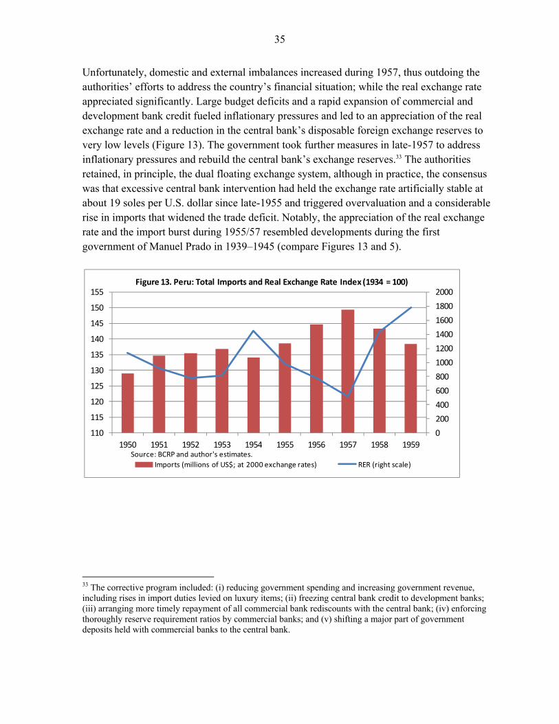
35

Unfortunately, domestic and external imbalances increased during 1957, thus outdoing the authorities’ efforts to address the country’s financial situation; while the real exchange rate appreciated significantly. Large budget deficits and a rapid expansion of commercial and development bank credit fueled inflationary pressures and led to an appreciation of the real exchange rate and a reduction in the central bank’s disposable foreign exchange reserves to very low levels (Figure 13). The government took further measures in late-1957 to address inflationary pressures and rebuild the central bank’s exchange reserves.33 The authorities retained, in principle, the dual floating exchange system, although in practice, the consensus was that excessive central bank intervention had held the exchange rate artificially stable at about 19 soles per U.S. dollar since late-1955 and triggered overvaluation and a considerable rise in imports that widened the trade deficit. Notably, the appreciation of the real exchange rate and the import burst during 1955/57 resembled developments during the first government of Manuel Prado in 1939–1945 (compare Figures 13 and 5).

33 The corrective program included: (i) reducing government spending and increasing government revenue, including rises in import duties levied on luxury items; (ii) freezing central bank credit to development banks; (iii) arranging more timely repayment of all commercial bank rediscounts with the central bank; (iv) enforcing thoroughly reserve requirement ratios by commercial banks; and (v) shifting a major part of government deposits held with commercial banks to the central bank.

0

200

400

600

800

1000

1200

1400

1600

1800

2000

110

115

120

125

130

135

140

145

150

155

1950 1951 1952 1953 1954 1955 1956 1957 1958 1959

Figure 13. Peru: Total Imports and Real Exchange Rate Index (1934 = 100)

Imports (millions of US$; at 2000 exchange rates) RER (right scale)

Source: BCRP and author's estimates.

36

To reinforce their economic program, the Prado administration went back to the IMF in February 1958, committing to enhanced exchange rate flexibility.34 The stakes were high because the fiscal deficit remained rather large, the external environment was not buoyant owing to a reduction in international prices for copper and zinc, and there were signs of capital flight. However, Peru’s sound policy implementation since the first Stand-By Arrangement in February 1954 pondered heavily in the IMF’s agreeing to a new program, which was complemented by a line of credit from the U.S. Treasury for US$17.5 million and a line of credit from a consortium of American banks for an equal amount. The understanding was that the authorities would not use their reserves and/or the foreign credit amounts to maintain an artificially low exchange rate, but rather would allow the exchange certificate market rate find its equilibrium level in an orderly manner (i.e., supported by a comprehensive fiscal and credit policy package) and permit an appropriate reserve accumulation. Lax fiscal policy out-weighted the 1958 stabilization efforts, and the Peruvian authorities embarked on yet another IMF-supported program in February 1959, which eventually delivered price and exchange rate stability. 35 This was the sixth year in a row of Fund-supported stabilization programs. As in the past, the arrangement was to be complemented by

34 The Stand-By Arrangement was for an amount of US$25 million (i.e., twice the size of the 1954 arrangement and equal to 100 percent of Peru’s quota with the IMF). See, SM/57/99, 1957 Consultations – Peru, 12/6/1957, IMF Archives; EBM/58/45, Use of Fund’s Resources – Stand-By Arrangement with Peru, 9/12/1958, IMF Archives.

35 See, EBM/59/3, Use of the Fund’s Resources – Stand –By Arrangement with Peru, 2/11/1959, IMF Archives; EBM/59/6, Peru – 1958 Consultations and Use of Fund’s Resources, 2/27/1959, IMF Archives; and EBS/59/13, Request for Stand-By Arrangement – Peru, 2/24/1959, IMF Archives.

60

80

100

120

140

160

1950 1951 1952 1953 1954 1955 1956 1957 1958 1959

Figure 14. Peru: Cost of Living and Nominal Exchange Rate, 1950/59 (Indices, 1955=100)

Exchange rate Cost of living

Source: BCRP and author's estimates.

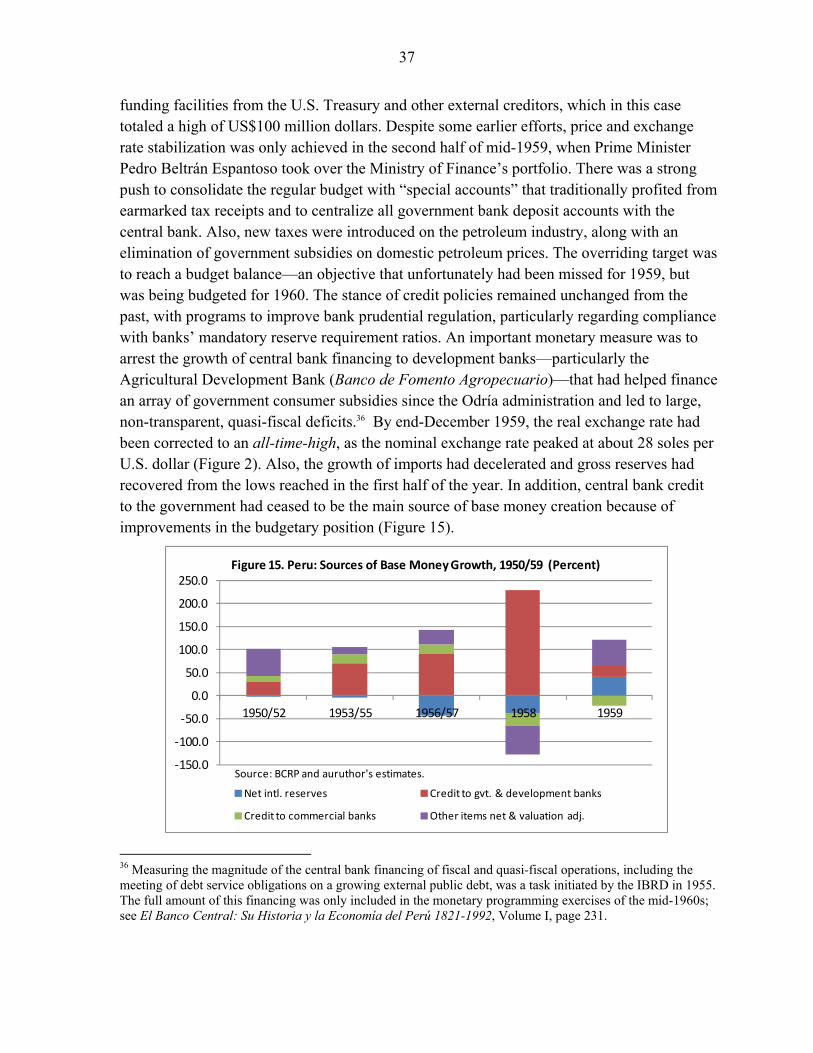
37

funding facilities from the U.S. Treasury and other external creditors, which in this case totaled a high of US$100 million dollars. Despite some earlier efforts, price and exchange rate stabilization was only achieved in the second half of mid-1959, when Prime Minister Pedro Beltrán Espantoso took over the Ministry of Finance’s portfolio. There was a strong push to consolidate the regular budget with “special accounts” that traditionally profited from earmarked tax receipts and to centralize all government bank deposit accounts with the central bank. Also, new taxes were introduced on the petroleum industry, along with an elimination of government subsidies on domestic petroleum prices. The overriding target was to reach a budget balance—an objective that unfortunately had been missed for 1959, but was being budgeted for 1960. The stance of credit policies remained unchanged from the past, with programs to improve bank prudential regulation, particularly regarding compliance with banks’ mandatory reserve requirement ratios. An important monetary measure was to arrest the growth of central bank financing to development banks—particularly the Agricultural Development Bank (Banco de Fomento Agropecuario)—that had helped finance an array of government consumer subsidies since the Odría administration and led to large, non-transparent, quasi-fiscal deficits.36 By end-December 1959, the real exchange rate had been corrected to an all-time-high, as the nominal exchange rate peaked at about 28 soles per U.S. dollar (Figure 2). Also, the growth of imports had decelerated and gross reserves had recovered from the lows reached in the first half of the year. In addition, central bank credit to the government had ceased to be the main source of base money creation because of improvements in the budgetary position (Figure 15).

36 Measuring the magnitude of the central bank financing of fiscal and quasi-fiscal operations, including the meeting of debt service obligations on a growing external public debt, was a task initiated by the IBRD in 1955. The full amount of this financing was only included in the monetary programming exercises of the mid-1960s; see El Banco Central: Su Historia y la Economía del Perú 1821-1992, Volume I, page 231.

-150.0

-100.0

-50.0

0.0

50.0

100.0

150.0

200.0

250.0

1950/52 1953/55 1956/57 1958 1959

Figure 15. Peru: Sources of Base Money Growth, 1950/59 (Percent)

Net intl. reserves Credit to gvt. & development banks

Credit to commercial banks Other items net & valuation adj.

Source: BCRP and auruthor's estimates.

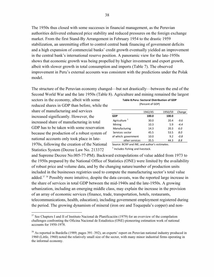
38

The 1950s thus closed with some successes in financial management, as the Peruvian authorities delivered enhanced price stability and reduced pressures on the foreign exchange market. From the first Stand-By Arrangement in February 1954 to the drastic 1959 stabilization, an unremitting effort to control central bank financing of government deficits and a high expansion of commercial banks’ credit growth eventually yielded an improvement in the central bank’s international reserve position. A panoramic view for the late-1950s shows that economic growth was being propelled by higher investment and export growth, albeit with slower growth in total consumption and imports (Table 7). The observed improvement in Peru’s external accounts was consistent with the predictions under the Polak model. The structure of the Peruvian economy changed—but not drastically—between the end of the Second World War and the late 1950s (Table 8). Agriculture and mining remained the largest sectors in the economy, albeit with some reduced shares in GDP than before, while the share of manufacturing and services increased significantly. However, the increased share of manufacturing in total GDP has to be taken with some reservation because the production of a robust system of national accounts only took place in late-1970s, following the creation of the National Statistics System (Decree Law No. 213372 and Supreme Decree No.005-77-PM). Backward extrapolations of value added from 1973 to the 1950s prepared by the National Office of Statistics (ONE) were limited by the availability of robust price and volume data, and by the changing nature/number of production units included in the businesses registries used to compute the manufacturing sector’s total value added.37 38 Possibly more intuitive, despite the data caveats, was the reported large increase in the share of services in total GDP between the mid-1940s and the late-1950s. A growing urbanization, including an emerging middle class, may explain the increase in the provision of an array of economic services (finance, trade, transportation, hotels, restaurants, telecommunications, health, education), including government employment registered during the period. The growing dynamism of mineral (iron ore and Toquepala’s copper) and non-

37 See Chapters I and II of Instituto Nacional de Planificación (1979) for an overview of the compilation challenges confronting the Oficina Nacional de Estadística (ONE) pioneering estimation work of national accounts for 1950-1978.

38 As reported in Bardella (1989; pages 391–392), an experts’ report on Peruvian national industry produced in 1960 (Little, 1960) noted the relatively small size of the sector, with many minor industrial firms operating in the informal economy.

1942/45 1950/59 Change

GDP 100.0 100.0

Agriculture 1 30.0 20.4 -9.6

Mining 10.3 5.9 -4.4

Manufacturing 14.3 20.3 6.0

Services sector 45.5 53.5 8.0

of which: government 10.0 9.2 -0.8

other services 35.5 44.3 8.8

Source: BCRP and INE; and author's estimates.1 Includes fishing and livestock.

(Percent of GDP)

Table 8.Peru: Sectoral Distribution of GDP

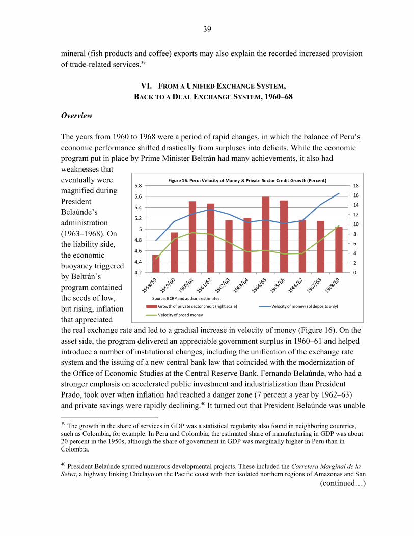
39

mineral (fish products and coffee) exports may also explain the recorded increased provision of trade-related services.39

VI. FROM A UNIFIED EXCHANGE SYSTEM, BACK TO A DUAL EXCHANGE SYSTEM, 1960–68

Overview The years from 1960 to 1968 were a period of rapid changes, in which the balance of Peru’s economic performance shifted drastically from surpluses into deficits. While the economic program put in place by Prime Minister Beltrán had many achievements, it also had weaknesses that eventually were magnified during President Belaúnde’s administration (1963–1968). On the liability side, the economic buoyancy triggered by Beltrán’s program contained the seeds of low, but rising, inflation that appreciated the real exchange rate and led to a gradual increase in velocity of money (Figure 16). On the asset side, the program delivered an appreciable government surplus in 1960–61 and helped introduce a number of institutional changes, including the unification of the exchange rate system and the issuing of a new central bank law that coincided with the modernization of the Office of Economic Studies at the Central Reserve Bank. Fernando Belaúnde, who had a stronger emphasis on accelerated public investment and industrialization than President Prado, took over when inflation had reached a danger zone (7 percent a year by 1962–63) and private savings were rapidly declining.40 It turned out that President Belaúnde was unable

39 The growth in the share of services in GDP was a statistical regularity also found in neighboring countries, such as Colombia, for example. In Peru and Colombia, the estimated share of manufacturing in GDP was about 20 percent in the 1950s, although the share of government in GDP was marginally higher in Peru than in Colombia.

40 President Belaúnde spurred numerous developmental projects. These included the Carretera Marginal de la Selva, a highway linking Chiclayo on the Pacific coast with then isolated northern regions of Amazonas and San

(continued…)

0

2

4

6

8

10

12

14

16

18

4.2

4.4

4.6

4.8

5

5.2

5.4

5.6

5.8Figure 16. Peru: Velocity of Money & Private Sector Credit Growth (Percent)

Growth of private sector credit (right scale) Velocity of money (sol deposits only)

Velocity of broad money

Source: BCRP and author's estimates.

40

to control inflation, which rose from 7 percent in 1962, to 17 percent in 1965, before reaching about 20 percent in 1968. The fiscal deficit ballooned, while a sizeable short-term external public sector debt put pressure on the budget and central bank international reserves. In September 1967, the sol was seriously devalued after a long period of currency overvaluation that had fostered rapid import growth and hurt export competitiveness. Unfortunately, the exchange rate action was not supported by a strong fiscal consolidation effort. President Belaúnde was deposed from office by the military junta led by General Juan Velasco Alvarado on October 3, 1968. A number of institutional constraints on the fiscal and monetary fronts weakened the Belaúnde administration’s stabilization efforts.41 First, the government had no majority in congress, which rejected most of the revenue-raising measures included in the programs agreed to with the IMF. Second, the budgetary system was fragmented, thus resulting in an array of ill-defined financial transfers between different levels of government (central and local governments), and between the central government and extrabudgetary units (e.g., public enterprises, the social security system, and development banks), that complicated the proper measurement of the fiscal stance. Third, despite earlier reform efforts, there was not a government consolidated bank account with the central bank. Rather, the budgetary and extra budgetary units held large deposits with commercial banks that supported a rapid increase in credit to the economy. Transferring these public sector bank deposits to the central bank (or even to the state development banks) became an important policy direction to prevent an excessive credit expansion by commercial banks and to develop a unified metering of the financing needs/sources of the public sector deficit. An additional consideration was that among the state development banks, the Agricultural Development Bank relied on central bank rediscounts to finance its operations, a source of credit expansion that the government found difficult to stop. Policy highlights The economic program launched by Prime Minister Beltrán in late 1959 improved fiscal and monetary management, abolished remaining exchange and trade restrictions, and began

Martín. He also advanced the ambitious Santiago Antunez de Mayolo and Chira Piura irrigation projects, and the Tinajones, Jequetepeque, Majes, Chavimochic, Olmos, Chinecas hydroelectric projects. Belaúnde also promoted a program of "social interest" homes in Lima and other cities, which benefited dozen of thousands of families.

41 See also Kuczynski (1977) for an account of the institutional weakness and challenges confronting the Belaúnde administration in the economic and political spheres.

41

focusing on development planning and social issues.42 The Beltrán economic program arrested the central government’s recourse to central bank financing and, together with a number of revenue raising and expenditure control measures, set the stage for fiscal surpluses in 1960-1961. Credit policy remained broadly tight during the period with strict monitoring/enforcing of commercial banks’ legal reserve requirements and penalties, although central bank financing of the agricultural development bank was an important source of money creation throughout the period. All in all, the economy grew at rates of 12 percent and 7 percent in 1960 and 1961, respectively, supported by a rapid growth in iron and copper exports, as well as sugar, fish, and fishmeal exports. The strong export growth, coupled with a resumption of capital inflows for the financing of large public and private investment projects, led to an increase in central bank official reserves, albeit to no more than two months of imports of goods and services. Inflation, as measured by the cost of living index, remained in the low single digit range in 1960–61, but it began to edge up in mid-1961, as overall economic activity accelerated and bank credit to the private sector rose rapidly during the period. At that time, inflation concerns also derived from the cost-push effect of numerous labor strikes and wage increases beyond productivity gains in the public and private sector, although the economics discussion lacked a strong analytical framework.43 A development plan prepared by the Economics Studies Department of the Peruvian Central Bank became an important blueprint for future structural reforms in terms of rural agricultural development, irrigation, roads, housing, and other infrastructure projects aimed at addressing the notable income per capita disparities between Lima, and a few coastal urban centers, and the rest of the country.44 The unification of the exchange market in May 1960 and the issuing of a new Central Bank Law in 1961 were important milestones in the early 1960s, further buttressing the support

42 See, EBM/61/4, Peru – Acceptance of Obligations of Article VIII, Sections 2, 3, and 4, 2/8/1961, IMF Archives; EBM/60/7, Peru – 1959 Consultations and Use of the Fund’s Resources, 2/29/1960; SM/60/40, Peru – Unification of Exchange Markets, 5/25/1960, IMF Archives; SM/61/9, Peru – 1960 Consultations, 2/14/1961, IMF Archives; EBM/62/8, Peru – 1961 Article VIII Consultations and Stand-By Arrangement, 2/26/1962; EBS/62/17, Peru – Request for Stand-By Arrangement, 2/15/1962, IMF Archives; EBS/63/24, Peru – Request for Stand-By Arrangement, 2/14/1963, IMF Archives; EBM/63/7, Peru – 1962 Article VIII Consultations and Stand-By Arrangement, 2/25/1963.

43There were numerous debates about the merits and challenges of wage controls to address the reported cost-push inflation. However, very few participants suggested that, possibly, wage pressures were induced, secondary sources of inflation, and the original cause was the booming mineral export sector. The logic was that an increase in the exploitation of natural resources is usually accompanied by increased demand for and prices of non-tradable goods that leads to overall inflation, appreciates the real exchange rate, and triggers wage demands. Unfortunately, the formalization of the “Dutch Disease” economic model only happened in 1982, with the seminal work by Max Corden and Peter Neary that was published in The Economic Journal.

44 Banco Central de Reserve del Perú (1961), Plan Naciónal de Desarrollo Económico y Social del Perú, 1962-1971, Tomo 1, 500 pages. See also, Webb (2009).

42

from the international financial community. A unified exchange market, with a single fluctuating rate of exchange, replaced the dual exchange rate system of an export certificate and a draft market exchange rate that was established in November 1949. However, no new par value for the sol against the U.S. dollar was established, because the government asserted that the stabilization process was still fragile and too vulnerable to support a new par value without recourse to trade and exchange restrictions. Also, international reserves remained relatively low for the central bank to defend any given parity in the event of ensuing internal and/or external disequilibria. A new Central Bank Law enhanced the central bank’s independence from the central government and gave the monetary authority supervisory power over the enforcement of reserve requirements, which until then had been under the supervision of the Banking Superintendency. The IMF continued to support the Peruvian government’s stabilization efforts through a continuous renewal of one-year Stand-By Arrangements in 1960–65 (see Box 1). Recurrent concerns during the consultation process with the IMF, however, were the gradual, albeit steady increase in inflation (that was reaching 10 percent a year) and the rise in public external debt. The stock of public and publicly guaranteed debt had increased from US$292 million in 1960, to US$370 million in 1963, and US$440 million in 1965 (equivalent to some 10 percent of GDP). External debt service payment obligations also had been on the rise since 1961, as the earlier vintage of private FDI in the mining sector that started in the early 1950s, was coming to maturity. The conduct of monetary and financial policies profited from a strong analytically oriented Economic Studies Department at the Central Reserve Bank, which bolstered the public sector’s institution-building process during the 1960s. According to the minutes of the central bank’s board of directors, much emphasis was placed in increasing the bank’s human capital, while at the same time disseminating timely macroeconomic statistics in the central bank’s Weekly Note (Nota Semanal) that was launched in 1964.45 Also, in 1961, the central bank established its, now traditional, university extension course (Curso de Extensión Técnica para Universitarios) that housed and trained the country’s top university students in economics on macroeconomics and central bank issues for three to six months. Policy memoranda and detailed technical advice, most of which was published in the bank’s Review (Reseña Económica y Financiera), are testimony of the consistent economic advice provided to policymakers by the central bank’s “técnicos” through the turbulent years leading to the military coup of October 1968.46

45 As reported in El Banco Central: Su Historia y la Economía del Perú 1821-1992, Volume II, Chapter 5, pages 409, 509, 525, and others.

46 According to Kuczynski (1977), in general, throughout the Belaúnde administration the advice from the central bank was for a strong fiscal consolidation to safeguard the country’s international reserve position. Such advice was contrary to that from the Ministry of Finance’s and the Planning Office’s advisers, which had strong ideological influence from the U.N. Economic Commission for Latin America (ECLAC), who favored a more lax fiscal stance. The early 1960s were the heyday of the conflict between the so-called “ECLAC” and

(continued…)

43

President Fernando Belaúnde took over from the military junta on July 28, 1963, in a climate of looming economic strains, but placed a strong accent on accelerated public investment and industrialization.47 While the economic policies launched under Prime Minister Beltrán were still succeeding in controlling the fiscal position and supporting strong economic growth, the annual rate of inflation was edging up and there were signs of a gradual increase in the velocity of money (Figure 16). Bank credit to the private sector was rising rapidly despite repeated increases in legal reserve requirements. Emerging challenges for the new administration were the decline in agricultural production, labor unrest in the cities, and invasions in the countryside. Consistent with his political view, and with reported little interest in questions of macroeconomic balance, Belaúnde was quick to frame a strong push toward increased social overhead investment (road construction, irrigation and land reclamation, ports and airports, low cost housing, public health and education) and supported a process of industrialization based on newly established state-owned public enterprises engaged in the production of fertilizers, steel, cement, and hydro-electric power (Kuczynski,1977). Import-substituting private industry was supported through import tariff hikes, the granting of tax incentives to automobile assembly plants, and tax exemptions for new businesses established in the sparsely populated Loreto province (Amazon area). The public sector financed its investment program to a considerable extent by borrowing abroad.

“IMF” views, and the conflict between the Planning Office and the Central Bank tended to mirror the international institutional difference, according to Kuczynski (1977).

47 The military junta had deposed President Prado in the aftermath of the 1962 presidential elections on grounds of alleged fraud during the voting process.

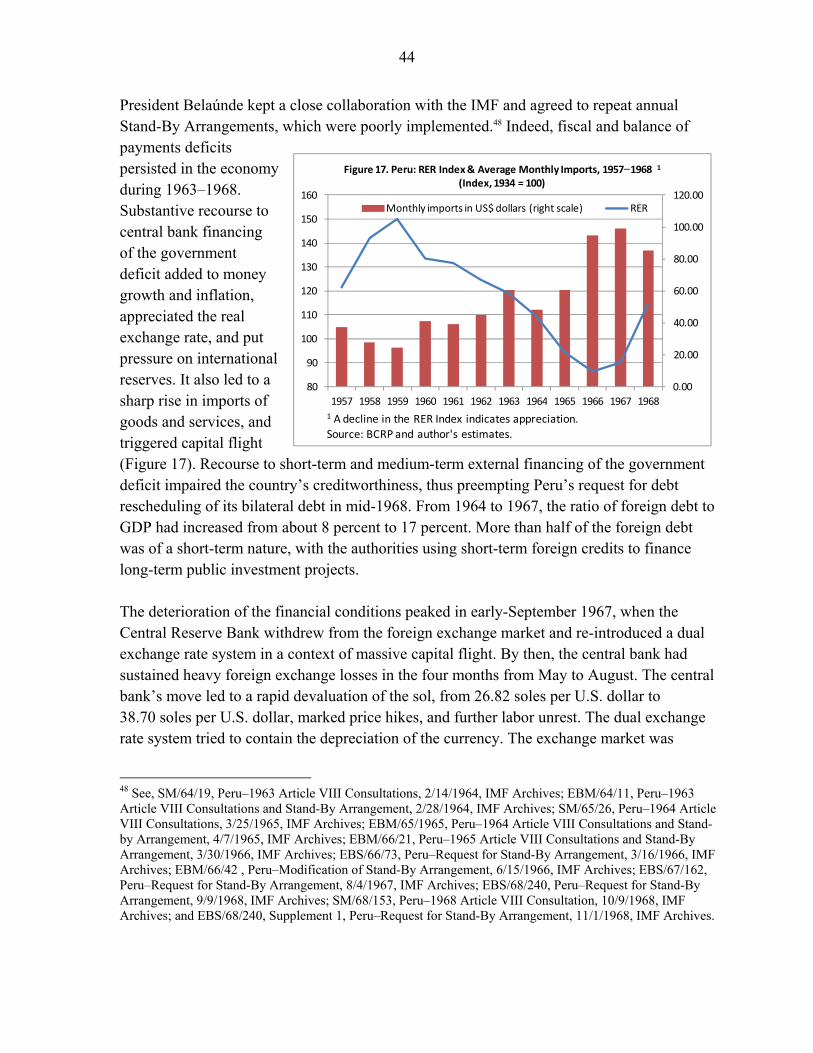
44

President Belaúnde kept a close collaboration with the IMF and agreed to repeat annual Stand-By Arrangements, which were poorly implemented.48 Indeed, fiscal and balance of payments deficits persisted in the economy during 1963–1968. Substantive recourse to central bank financing of the government deficit added to money growth and inflation, appreciated the real exchange rate, and put pressure on international reserves. It also led to a sharp rise in imports of goods and services, and triggered capital flight (Figure 17). Recourse to short-term and medium-term external financing of the government deficit impaired the country’s creditworthiness, thus preempting Peru’s request for debt rescheduling of its bilateral debt in mid-1968. From 1964 to 1967, the ratio of foreign debt to GDP had increased from about 8 percent to 17 percent. More than half of the foreign debt was of a short-term nature, with the authorities using short-term foreign credits to finance long-term public investment projects. The deterioration of the financial conditions peaked in early-September 1967, when the Central Reserve Bank withdrew from the foreign exchange market and re-introduced a dual exchange rate system in a context of massive capital flight. By then, the central bank had sustained heavy foreign exchange losses in the four months from May to August. The central bank’s move led to a rapid devaluation of the sol, from 26.82 soles per U.S. dollar to 38.70 soles per U.S. dollar, marked price hikes, and further labor unrest. The dual exchange rate system tried to contain the depreciation of the currency. The exchange market was

48 See, SM/64/19, Peru–1963 Article VIII Consultations, 2/14/1964, IMF Archives; EBM/64/11, Peru–1963 Article VIII Consultations and Stand-By Arrangement, 2/28/1964, IMF Archives; SM/65/26, Peru–1964 Article VIII Consultations, 3/25/1965, IMF Archives; EBM/65/1965, Peru–1964 Article VIII Consultations and Stand-by Arrangement, 4/7/1965, IMF Archives; EBM/66/21, Peru–1965 Article VIII Consultations and Stand-By Arrangement, 3/30/1966, IMF Archives; EBS/66/73, Peru–Request for Stand-By Arrangement, 3/16/1966, IMF Archives; EBM/66/42 , Peru–Modification of Stand-By Arrangement, 6/15/1966, IMF Archives; EBS/67/162, Peru–Request for Stand-By Arrangement, 8/4/1967, IMF Archives; EBS/68/240, Peru–Request for Stand-By Arrangement, 9/9/1968, IMF Archives; SM/68/153, Peru–1968 Article VIII Consultation, 10/9/1968, IMF Archives; and EBS/68/240, Supplement 1, Peru–Request for Stand-By Arrangement, 11/1/1968, IMF Archives.

0.00

20.00

40.00

60.00

80.00

100.00

120.00

80

90

100

110

120

130

140

150

160

1957 1958 1959 1960 1961 1962 1963 1964 1965 1966 1967 1968

Figure 17. Peru: RER Index & Average Monthly Imports, 1957−1968 1

(Index, 1934 = 100)

Monthly imports in US$ dollars (right scale) RER

1 A decline in the RER Index indicates appreciation.

Source: BCRP and author's estimates.

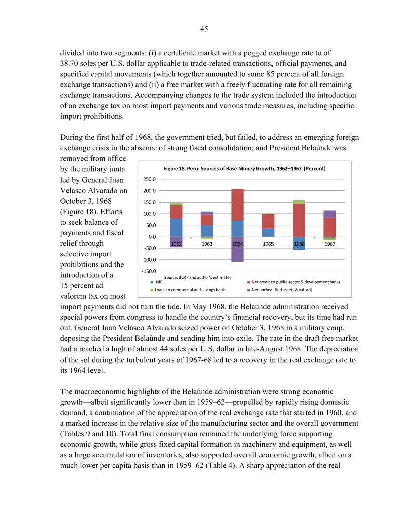
45

divided into two segments: (i) a certificate market with a pegged exchange rate to of 38.70 soles per U.S. dollar applicable to trade-related transactions, official payments, and specified capital movements (which together amounted to some 85 percent of all foreign exchange transactions) and (ii) a free market with a freely fluctuating rate for all remaining exchange transactions. Accompanying changes to the trade system included the introduction of an exchange tax on most import payments and various trade measures, including specific import prohibitions. During the first half of 1968, the government tried, but failed, to address an emerging foreign exchange crisis in the absence of strong fiscal consolidation; and President Belaúnde was removed from office by the military junta led by General Juan Velasco Alvarado on October 3, 1968 (Figure 18). Efforts to seek balance of payments and fiscal relief through selective import prohibitions and the introduction of a 15 percent ad valorem tax on most import payments did not turn the tide. In May 1968, the Belaúnde administration received special powers from congress to handle the country’s financial recovery, but its time had run out. General Juan Velasco Alvarado seized power on October 3, 1968 in a military coup, deposing the President Belaúnde and sending him into exile. The rate in the draft free market had a reached a high of almost 44 soles per U.S. dollar in late-August 1968. The depreciation of the sol during the turbulent years of 1967-68 led to a recovery in the real exchange rate to its 1964 level. The macroeconomic highlights of the Belaúnde administration were strong economic growth—albeit significantly lower than in 1959–62—propelled by rapidly rising domestic demand, a continuation of the appreciation of the real exchange rate that started in 1960, and a marked increase in the relative size of the manufacturing sector and the overall government (Tables 9 and 10). Total final consumption remained the underlying force supporting economic growth, while gross fixed capital formation in machinery and equipment, as well as a large accumulation of inventories, also supported overall economic growth, albeit on a much lower per capita basis than in 1959–62 (Table 4). A sharp appreciation of the real

-150.0

-100.0

-50.0

0.0

50.0

100.0

150.0

200.0

250.0

1962 1963 1964 1965 1966 1967

Figure 18. Peru: Sources of Base Money Growth, 1962−1967 (Percent)

NIR Net credit to public sector & development banks

Loans to commercial and savings banks Net unclassified assets & val. adj.

Source: BCRP and author's estimates.

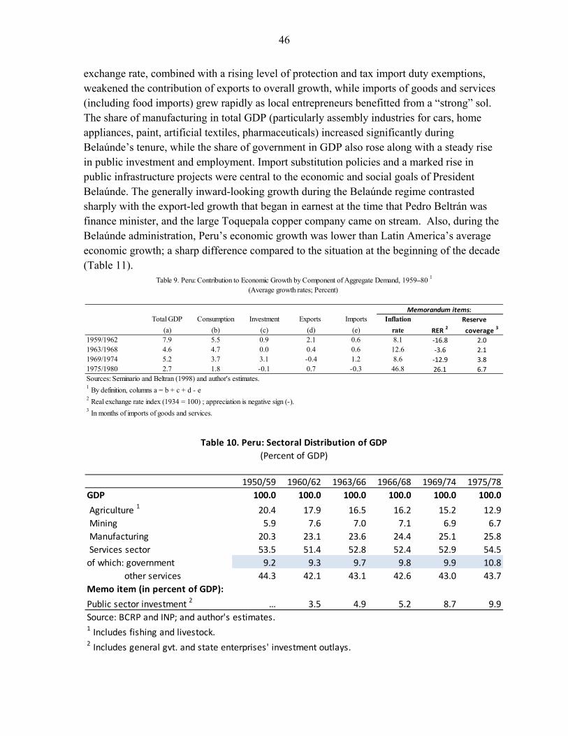
46

exchange rate, combined with a rising level of protection and tax import duty exemptions, weakened the contribution of exports to overall growth, while imports of goods and services (including food imports) grew rapidly as local entrepreneurs benefitted from a “strong” sol. The share of manufacturing in total GDP (particularly assembly industries for cars, home appliances, paint, artificial textiles, pharmaceuticals) increased significantly during Belaúnde’s tenure, while the share of government in GDP also rose along with a steady rise in public investment and employment. Import substitution policies and a marked rise in public infrastructure projects were central to the economic and social goals of President Belaúnde. The generally inward-looking growth during the Belaúnde regime contrasted sharply with the export-led growth that began in earnest at the time that Pedro Beltrán was finance minister, and the large Toquepala copper company came on stream. Also, during the Belaúnde administration, Peru’s economic growth was lower than Latin America’s average economic growth; a sharp difference compared to the situation at the beginning of the decade (Table 11).

Total GDP Consumption Investment Exports Imports Inflation Reserve

(a) (b) (c) (d) (e) rate RER 2 coverage 3

1959/1962 7.9 5.5 0.9 2.1 0.6 8.1 -16.8 2.0

1963/1968 4.6 4.7 0.0 0.4 0.6 12.6 -3.6 2.1

1969/1974 5.2 3.7 3.1 -0.4 1.2 8.6 -12.9 3.8

1975/1980 2.7 1.8 -0.1 0.7 -0.3 46.8 26.1 6.7

Sources: Seminario and Beltran (1998) and author's estimates.1 By definition, columns a = b + c + d - e2 Real exchange rate index (1934 = 100) ; appreciation is negative sign (-).3 In months of imports of goods and services.

Memorandum items:

Table 9. Peru: Contribution to Economic Growth by Component of Aggregate Demand, 1959–80 1

(Average growth rates; Percent)

1950/59 1960/62 1963/66 1966/68 1969/74 1975/78

GDP 100.0 100.0 100.0 100.0 100.0 100.0

Agriculture 1 20.4 17.9 16.5 16.2 15.2 12.9

Mining 5.9 7.6 7.0 7.1 6.9 6.7

Manufacturing 20.3 23.1 23.6 24.4 25.1 25.8

Services sector 53.5 51.4 52.8 52.4 52.9 54.5

of which: government 9.2 9.3 9.7 9.8 9.9 10.8

other services 44.3 42.1 43.1 42.6 43.0 43.7

Memo item (in percent of GDP):

Public sector investment 2 … 3.5 4.9 5.2 8.7 9.9

Source: BCRP and INP; and author's estimates.1 Includes fishing and livestock.2 Includes general gvt. and state enterprises' investment outlays.

Table 10. Peru: Sectoral Distribution of GDP

(Percent of GDP)

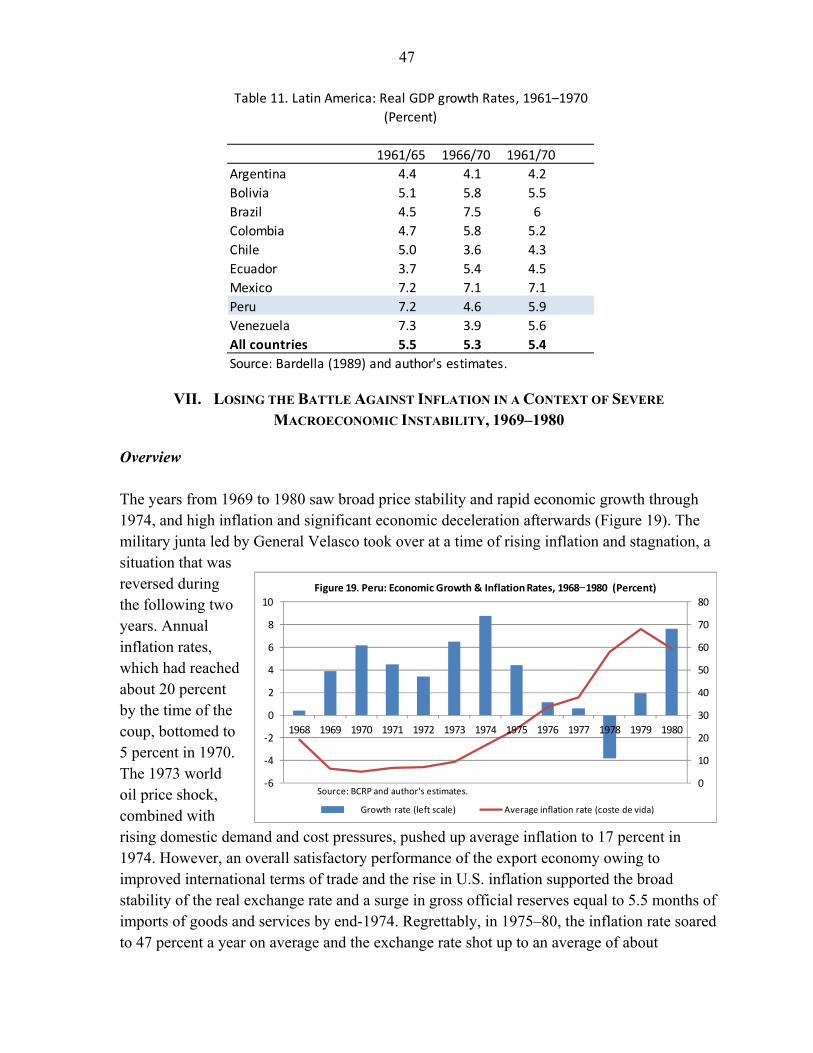
47

VII. LOSING THE BATTLE AGAINST INFLATION IN A CONTEXT OF SEVERE

MACROECONOMIC INSTABILITY, 1969–1980

Overview The years from 1969 to 1980 saw broad price stability and rapid economic growth through 1974, and high inflation and significant economic deceleration afterwards (Figure 19). The military junta led by General Velasco took over at a time of rising inflation and stagnation, a situation that was reversed during the following two years. Annual inflation rates, which had reached about 20 percent by the time of the coup, bottomed to 5 percent in 1970. The 1973 world oil price shock, combined with rising domestic demand and cost pressures, pushed up average inflation to 17 percent in 1974. However, an overall satisfactory performance of the export economy owing to improved international terms of trade and the rise in U.S. inflation supported the broad stability of the real exchange rate and a surge in gross official reserves equal to 5.5 months of imports of goods and services by end-1974. Regrettably, in 1975–80, the inflation rate soared to 47 percent a year on average and the exchange rate shot up to an average of about

1961/65 1966/70 1961/70

Argentina 4.4 4.1 4.2

Bolivia 5.1 5.8 5.5

Brazil 4.5 7.5 6

Colombia 4.7 5.8 5.2

Chile 5.0 3.6 4.3

Ecuador 3.7 5.4 4.5

Mexico 7.2 7.1 7.1

Peru 7.2 4.6 5.9

Venezuela 7.3 3.9 5.6

All countries 5.5 5.3 5.4

Source: Bardella (1989) and author's estimates.

Table 11. Latin America: Real GDP growth Rates, 1961–1970

(Percent)

0

10

20

30

40

50

60

70

80

-6

-4

-2

0

2

4

6

8

10

1968 1969 1970 1971 1972 1973 1974 1975 1976 1977 1978 1979 1980

Figure 19. Peru: Economic Growth & Inflation Rates, 1968−1980 (Percent)

Growth rate (left scale) Average inflation rate (coste de vida)

Source: BCRP and author's estimates.

48

173 soles per U.S. dollar, compared with 43 soles per dollar in 1968–74. International reserve coverage improved by the end of the decade and the level of the real exchange rate was higher (more competitive) than in 1975, although, by then, the economy was severely battered by the 1977–78 stagnation, dwindling money demand, and unremitting capital flight. It was not a happy ending for the 1970s. Peru’s intense relationship with the IMF changed somewhat in the 1968–1977. In 1971, the Peruvian authorities did not sign a new Stand-By Arrangement with the IMF, thus ending 16 years of continuous financial arrangements with the Bretton Woods institution. The authorities did, however, have recourse to IMF financial support under the IMF facilities on Compensatory Financing of Export Fluctuations (in 1972 and 1976) and the Oil Facility (1976). Financial support covered balance of payments shortfalls stemming from sharp swings of international demand and prices for exports (minerals and fishmeal) and imports (oil) that emerged during the period. Peru also drew IMF financial support under the country’s Gold Tranche and the First Credit Tranche (1976) with the IMF. Policy conditionality under these facilities was relatively limited compared to that under standard IMF Stand-By Arrangements.49 Stand-By Arrangements with the Fund only resumed in late-1977 in the context of domestic and international efforts to restore Peru’s deteriorated international reserve position and avoid default of its external debt obligations. Four consecutive arrangements in support of the government’s stabilization program were put in place between October 1977 and December 1980.50 The stabilization programs, which included major revisions of exchange rate and tax policies, elimination of consumer subsidies, and cuts in overall public spending, improved the fiscal and balance of payments positions, although the average annual rate of inflation reached all-time highs (in the range of 60 to 70 percent a year) and the economy stagnated in 1977–1979.

49 Borrowing countries under the compensatory financing facility, the oil and gold tranches, and the first credit tranche, were only required to present to the IMF an economic program indicating a reasonable effort to find appropriate solutions to their balance of payments difficulties. Also, under the compensatory financing facility, borrowers needed to demonstrate that the export shortfall was of a short-term character and due to factors largely beyond the borrower’s control. By contrast, conditionality under the traditional Stand-By Arrangements included the fulfillment of strict quantitative financial benchmarks and targets, as well as prior actions on critical macroeconomic areas/policies, as pre-conditions for IMF financial disbursements. See, EBS/72/178, Peru – Use of Fund’s Resources, 6/1/1972, IMF Archives; EBS/72/178, Supplement 1, Peru – Purchase Transaction, 6/14/1972, IMF Archives; and EBS/76/173, Peru – Use of Fund Resources – Compensatory Financing, 4/16/1976, IMF Archives.

50 Peru also received financing under the IMF Compensatory Financing Facility in late 1978. Drawings under the facility sought to address Peru’s export shortfalls of petroleum and derivates, and fish and agricultural products.

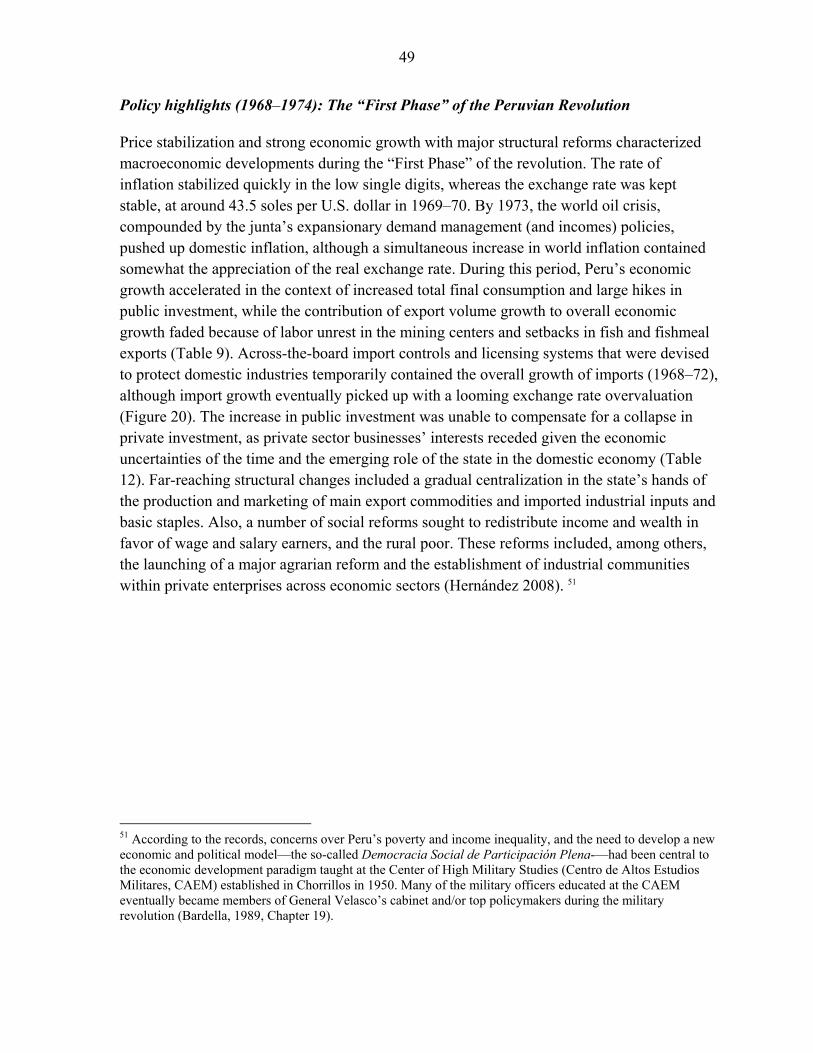
49

Policy highlights (1968–1974): The “First Phase” of the Peruvian Revolution

Price stabilization and strong economic growth with major structural reforms characterized macroeconomic developments during the “First Phase” of the revolution. The rate of inflation stabilized quickly in the low single digits, whereas the exchange rate was kept stable, at around 43.5 soles per U.S. dollar in 1969–70. By 1973, the world oil crisis, compounded by the junta’s expansionary demand management (and incomes) policies, pushed up domestic inflation, although a simultaneous increase in world inflation contained somewhat the appreciation of the real exchange rate. During this period, Peru’s economic growth accelerated in the context of increased total final consumption and large hikes in public investment, while the contribution of export volume growth to overall economic growth faded because of labor unrest in the mining centers and setbacks in fish and fishmeal exports (Table 9). Across-the-board import controls and licensing systems that were devised to protect domestic industries temporarily contained the overall growth of imports (1968–72), although import growth eventually picked up with a looming exchange rate overvaluation (Figure 20). The increase in public investment was unable to compensate for a collapse in private investment, as private sector businesses’ interests receded given the economic uncertainties of the time and the emerging role of the state in the domestic economy (Table 12). Far-reaching structural changes included a gradual centralization in the state’s hands of the production and marketing of main export commodities and imported industrial inputs and basic staples. Also, a number of social reforms sought to redistribute income and wealth in favor of wage and salary earners, and the rural poor. These reforms included, among others, the launching of a major agrarian reform and the establishment of industrial communities within private enterprises across economic sectors (Hernández 2008). 51

51 According to the records, concerns over Peru’s poverty and income inequality, and the need to develop a new economic and political model—the so-called Democracia Social de Participación Plena-—had been central to the economic development paradigm taught at the Center of High Military Studies (Centro de Altos Estudios Militares, CAEM) established in Chorrillos in 1950. Many of the military officers educated at the CAEM eventually became members of General Velasco’s cabinet and/or top policymakers during the military revolution (Bardella, 1989, Chapter 19).

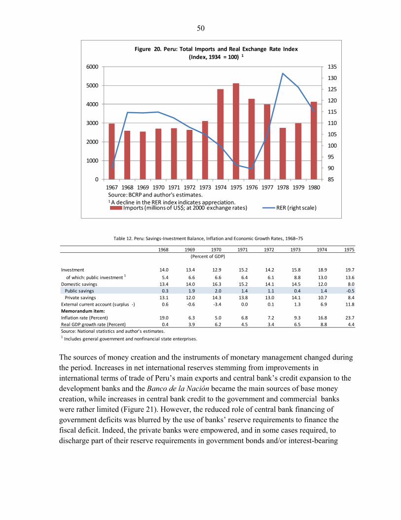
50

The sources of money creation and the instruments of monetary management changed during the period. Increases in net international reserves stemming from improvements in international terms of trade of Peru’s main exports and central bank’s credit expansion to the development banks and the Banco de la Nación became the main sources of base money creation, while increases in central bank credit to the government and commercial banks were rather limited (Figure 21). However, the reduced role of central bank financing of government deficits was blurred by the use of banks’ reserve requirements to finance the fiscal deficit. Indeed, the private banks were empowered, and in some cases required, to discharge part of their reserve requirements in government bonds and/or interest-bearing

1968 1969 1970 1971 1972 1973 1974 1975

Investment 14.0 13.4 12.9 15.2 14.2 15.8 18.9 19.7

of which: public investment 1 5.4 6.6 6.6 6.4 6.1 8.8 13.0 13.6

Domestic savings 13.4 14.0 16.3 15.2 14.1 14.5 12.0 8.0

Public savings 0.3 1.9 2.0 1.4 1.1 0.4 1.4 -0.5

Private savings 13.1 12.0 14.3 13.8 13.0 14.1 10.7 8.4

External current account (surplus -) 0.6 -0.6 -3.4 0.0 0.1 1.3 6.9 11.8

Memorandum item:

Inflation rate (Percent) 19.0 6.3 5.0 6.8 7.2 9.3 16.8 23.7

Real GDP growth rate (Percent) 0.4 3.9 6.2 4.5 3.4 6.5 8.8 4.4

Source: National statistics and author's estimates.1 Includes general government and nonfinancial state enterprises.

Table 12. Peru: Savings-Investment Balance, Inflation and Economic Growth Rates, 1968–75

(Percent of GDP)

85

90

95

100

105

110

115

120

125

130

135

0

1000

2000

3000

4000

5000

6000

1967 1968 1969 1970 1971 1972 1973 1974 1975 1976 1977 1978 1979 1980

Figure 20. Peru: Total Imports and Real Exchange Rate Index

(Index, 1934 = 100) 1

Imports (millions of US$; at 2000 exchange rates) RER (right scale)

Source: BCRP and author's estimates.1 A decline in the RER index indicates appreciation.

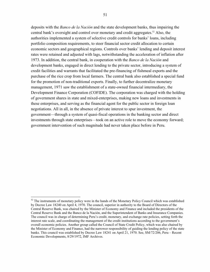
51

deposits with the Banco de la Nación and the state development banks, thus impairing the central bank’s oversight and control over monetary and credit aggregates.52 Also, the authorities implemented a system of selective credit controls for banks’ loans, including portfolio composition requirements, to steer financial sector credit allocation to certain economic sectors and geographical regions. Controls over banks’ lending and deposit interest rates were retained and adjusted with lags, notwithstanding the acceleration of inflation after 1973. In addition, the central bank, in cooperation with the Banco de la Nación and development banks, engaged in direct lending to the private sector, introducing a system of credit facilities and warrants that facilitated the pre-financing of fishmeal exports and the purchase of the rice crop from local farmers. The central bank also established a special fund for the promotion of non-traditional exports. Finally, to further decentralize monetary management, 1971 saw the establishment of a state-owned financial intermediary, the Development Finance Corporation (COFIDE). The corporation was charged with the holding of government shares in state and mixed-enterprises, making new loans and investments in these enterprises, and serving as the financial agent for the public sector in foreign loan negotiations. All in all, in the absence of private interest to spur investment, the government—through a system of quasi-fiscal operations in the banking sector and direct investments through state enterprises—took on an active role to move the economy forward; government intervention of such magnitude had never taken place before in Peru.

52 The instruments of monetary policy were in the hands of the Monetary Policy Council which was established by Decree Law 18240 on April 4, 1970. The council, superior in authority to the Board of Directors of the Central Reserve Bank, was chaired by the Minister of Economy and Finance and included the presidents of the Central Reserve Bank and the Banco de la Nación, and the Superintendent of Banks and Insurance Companies. The council was in charge of determining Peru’s credit, monetary, and exchange rate policies, setting forth the interest rate scale, and coordinating the management of the credit institutions according to the government’s overall economic policies. Another group called the Council of State Credit Policy, which was also chaired by the Minister of Economy and Finance, had the narrower responsibility of guiding the lending policy of the state banks. This council was established by Decree Law 18241 on April 21, 1970. See, SM/72/206, Peru – Recent Economic Developments, 8/29/1972, IMF Archives.

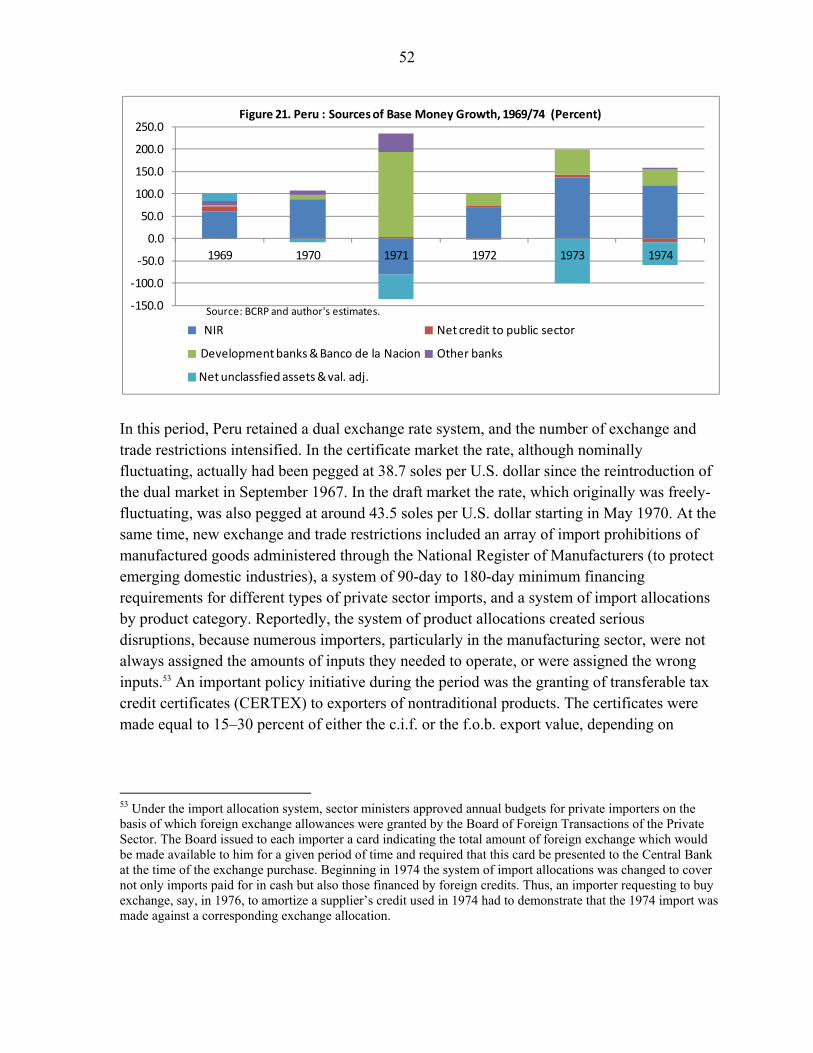
52

In this period, Peru retained a dual exchange rate system, and the number of exchange and trade restrictions intensified. In the certificate market the rate, although nominally fluctuating, actually had been pegged at 38.7 soles per U.S. dollar since the reintroduction of the dual market in September 1967. In the draft market the rate, which originally was freely-fluctuating, was also pegged at around 43.5 soles per U.S. dollar starting in May 1970. At the same time, new exchange and trade restrictions included an array of import prohibitions of manufactured goods administered through the National Register of Manufacturers (to protect emerging domestic industries), a system of 90-day to 180-day minimum financing requirements for different types of private sector imports, and a system of import allocations by product category. Reportedly, the system of product allocations created serious disruptions, because numerous importers, particularly in the manufacturing sector, were not always assigned the amounts of inputs they needed to operate, or were assigned the wrong inputs.53 An important policy initiative during the period was the granting of transferable tax credit certificates (CERTEX) to exporters of nontraditional products. The certificates were made equal to 15–30 percent of either the c.i.f. or the f.o.b. export value, depending on

53 Under the import allocation system, sector ministers approved annual budgets for private importers on the basis of which foreign exchange allowances were granted by the Board of Foreign Transactions of the Private Sector. The Board issued to each importer a card indicating the total amount of foreign exchange which would be made available to him for a given period of time and required that this card be presented to the Central Bank at the time of the exchange purchase. Beginning in 1974 the system of import allocations was changed to cover not only imports paid for in cash but also those financed by foreign credits. Thus, an importer requesting to buy exchange, say, in 1976, to amortize a supplier’s credit used in 1974 had to demonstrate that the 1974 import was made against a corresponding exchange allocation.

-150.0

-100.0

-50.0

0.0

50.0

100.0

150.0

200.0

250.0

1969 1970 1971 1972 1973 1974

Figure 21. Peru : Sources of Base Money Growth, 1969/74 (Percent)

NIR Net credit to public sector

Development banks & Banco de la Nacion Other banks

Net unclassfied assets & val. adj.

Source: BCRP and author's estimates.

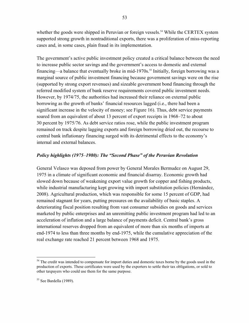
53

whether the goods were shipped in Peruvian or foreign vessels.54 While the CERTEX system supported strong growth in nontraditional exports, there was a proliferation of miss-reporting cases and, in some cases, plain fraud in its implementation. The government’s active public investment policy created a critical balance between the need to increase public sector savings and the government’s access to domestic and external financing—a balance that eventually broke in mid-1970s.55 Initially, foreign borrowing was a marginal source of public investment financing because government savings were on the rise (supported by strong export revenues) and sizeable government bond financing through the referred modified system of bank reserve requirements covered public investment needs. However, by 1974/75, the authorities had increased their reliance on external public borrowing as the growth of banks’ financial resources lagged (i.e., there had been a significant increase in the velocity of money; see Figure 16). Thus, debt service payments soared from an equivalent of about 13 percent of export receipts in 1968–72 to about 30 percent by 1975/76. As debt service ratios rose, while the public investment program remained on track despite lagging exports and foreign borrowing dried out, the recourse to central bank inflationary financing surged with its detrimental effects to the economy’s internal and external balances. Policy highlights (1975–1980): The “Second Phase” of the Peruvian Revolution General Velasco was deposed from power by General Morales Bermudez on August 29, 1975 in a climate of significant economic and financial disarray. Economic growth had slowed down because of weakening export value growth for copper and fishing products, while industrial manufacturing kept growing with import substitution policies (Hernández, 2008). Agricultural production, which was responsible for some 15 percent of GDP, had remained stagnant for years, putting pressures on the availability of basic staples. A deteriorating fiscal position resulting from vast consumer subsidies on goods and services marketed by public enterprises and an unremitting public investment program had led to an acceleration of inflation and a large balance of payments deficit. Central bank’s gross international reserves dropped from an equivalent of more than six months of imports at end-1974 to less than three months by end-1975, while the cumulative appreciation of the real exchange rate reached 21 percent between 1968 and 1975.

54 The credit was intended to compensate for import duties and domestic taxes borne by the goods used in the production of exports. These certificates were used by the exporters to settle their tax obligations, or sold to other taxpayers who could use them for the same purpose.

55 See Bardella (1989).

54

The government of General Morales Bermudez was quick to implement a stabilization program that, despite important reforms of the exchange system, failed to correct Peru’s internal and external balances. In late September 1975, the exchange rates in the certificate and free market were unified at a rate of 45 soles per U.S. dollar. The unification of the exchange market was complemented with revisions to the systems of minimum financing requirements of imports and import allocations to reduce economic distortions. However, by mid-1976, the program’s macroeconomic objectives had succumbed to the pursuit of expansionary monetary, fiscal and incomes policies that fed inflationary pressures and perpetuated large current account deficits of the balance of payments. A steady deterioration of the balance of payments culminated in a net international reserve loss of more than US$1.2 billion in the 18 months ending in June 1976, when the central bank’s net international reserve position dropped to negative US$500 million and the central bank was forced to temporarily close the foreign exchange market. An economic program launched in mid-1976 failed again to stabilize the economy, thus forcing the government to free the exchange rate in late-1977. The mid-1976 program included sizeable corrective price adjustments for gasoline and food staples to address the fiscal deficit and a large up-front exchange rate depreciation that was followed by a practice of depreciating the sol against the U.S. dollar once or twice a week. Nevertheless, an expansionary fiscal policy caused inflation to accelerate and led to a further large loss of net international reserves. By the end of the third quarter of 1977 the level of freely disposable foreign exchange reserves was reduced to the equivalent of a few days of imports. In early October 1977, the authorities developed a new stabilization program in cooperation with the IMF. The program abolished the system of import controls, adjusted prices and tariffs of some key public enterprises to catch up with past inflation, and freed the exchange market which, in combination, triggered a major devaluation of the sol (Figure 22). The government also announced accompanying fiscal and monetary policies to resume progress towards balance of payments equilibrium and to address domestic inflation, which had reached an average of about 45 percent in September 1977. Headline monetary measures included limits on overall banking sector credit expansion to the private and public sectors, and a policy of positive real interest rates to support an increase in money demand. The system of reserve requirements, which had already been simplified under the mid-1976 economic program, remained in place although the authorities stood ready to use this instrument as needed to control overall credit developments.

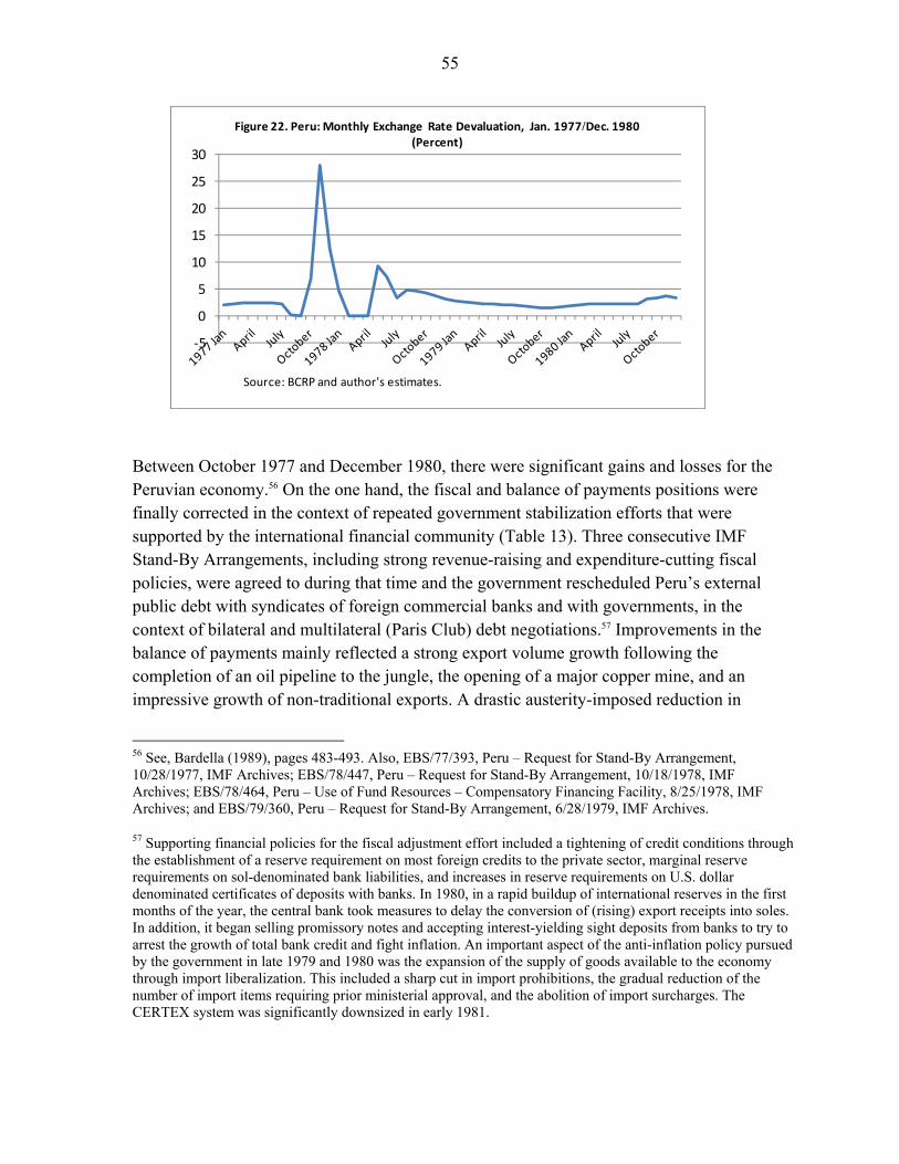
55

Between October 1977 and December 1980, there were significant gains and losses for the Peruvian economy.56 On the one hand, the fiscal and balance of payments positions were finally corrected in the context of repeated government stabilization efforts that were supported by the international financial community (Table 13). Three consecutive IMF Stand-By Arrangements, including strong revenue-raising and expenditure-cutting fiscal policies, were agreed to during that time and the government rescheduled Peru’s external public debt with syndicates of foreign commercial banks and with governments, in the context of bilateral and multilateral (Paris Club) debt negotiations.57 Improvements in the balance of payments mainly reflected a strong export volume growth following the completion of an oil pipeline to the jungle, the opening of a major copper mine, and an impressive growth of non-traditional exports. A drastic austerity-imposed reduction in

56 See, Bardella (1989), pages 483-493. Also, EBS/77/393, Peru – Request for Stand-By Arrangement, 10/28/1977, IMF Archives; EBS/78/447, Peru – Request for Stand-By Arrangement, 10/18/1978, IMF Archives; EBS/78/464, Peru – Use of Fund Resources – Compensatory Financing Facility, 8/25/1978, IMF Archives; and EBS/79/360, Peru – Request for Stand-By Arrangement, 6/28/1979, IMF Archives.

57 Supporting financial policies for the fiscal adjustment effort included a tightening of credit conditions through the establishment of a reserve requirement on most foreign credits to the private sector, marginal reserve requirements on sol-denominated bank liabilities, and increases in reserve requirements on U.S. dollar denominated certificates of deposits with banks. In 1980, in a rapid buildup of international reserves in the first months of the year, the central bank took measures to delay the conversion of (rising) export receipts into soles. In addition, it began selling promissory notes and accepting interest-yielding sight deposits from banks to try to arrest the growth of total bank credit and fight inflation. An important aspect of the anti-inflation policy pursued by the government in late 1979 and 1980 was the expansion of the supply of goods available to the economy through import liberalization. This included a sharp cut in import prohibitions, the gradual reduction of the number of import items requiring prior ministerial approval, and the abolition of import surcharges. The CERTEX system was significantly downsized in early 1981.

-5

0

5

10

15

20

25

30

Figure 22. Peru: Monthly Exchange Rate Devaluation, Jan. 1977/Dec. 1980 (Percent)

Source: BCRP and author's estimates.

56

imports added to the improvement in the external current account balance. On the other hand, progress in reducing the rate of inflation and reactivating the economy proved harder to attain. Average inflation remained persistently high—at about 60 percent on average in 1978–80—and the economy contracted in 1977–1978, albeit before recovering in 1979/80 on account of the export surge previously mentioned. Average incomes per-capita collapsed between 1970 and 1980, and private investment was at historical lows as a share of GDP. The social costs of the stabilization process were paramount as signaled by the poverty rates across the country and the exodus of Peruvians citizens to foreign countries in search of jobs and better living opportunities.

Exchange rate policy was revisited significantly during the 1977–1980 period. The initial floating of the exchange rate in October 1977 was followed by a policy of frequent mini-devaluations of the exchange rate (i.e., a crawling peg regime) starting in May 1978. After being maintained at 130 soles per U.S. dollar since December 1977, the exchange rate was devalued to 150 soles per U.S. dollar in May 1978; and since then the rate was adjusted steadily by the central bank in a series of frequent small (mini) depreciations (in line with the rate of domestic inflation), reaching 194 soles per U.S. dollar in December 1978. In January 1979, as an anti-inflationary measure, the rate of depreciation was slowed to roughly one half of the rate of domestic inflation or to approximately 2.5 percent per month on average. Beginning in February 1979, the authorities initiated a policy of announcing the exchange rate one month in advance, extending the announcement to two months in advance beginning in March. At the same time, in an attempt to influence expectations, the authorities let it be known which would be an appropriate end-year exchange rate level/target. In July 1980, under the newly elected government of Fernando Belaúnde, the preannounced exchange rate policy was abandoned. The new policy was to depreciate the sol frequently by small steps

1975 1976 1977 1978 1979 1980

Investment 19.7 17.8 15.0 14.6 14.6 17.8

of which: public investment 1 13.6 13.2 13.2 13.2 13.2 13.2

Domestic savings 8.0 10.3 8.5 14.1 21.3 18.7

Public savings -0.5 0.2 -3.7 -1.6 3.6 2.5

Private savings 8.4 10.1 12.2 15.7 17.7 16.3

External current account (surplus -) 11.8 7.5 6.6 0.5 -6.7 -1.0

Memorandum item:

Inflation rate (Percent) 23.7 33.6 38.0 58.1 67.9 59.4

Real GDP growth rate (Percent) 4.4 1.2 0.6 -3.8 2.0 7.7

Source: National statistics and author's estimates.1 Includes general government and nonfinancial state enterprises.

Table 13. Peru: Savings-Investment Balance, Inflation and Economic Growth Rates, 1975–80

(Percent of GDP)

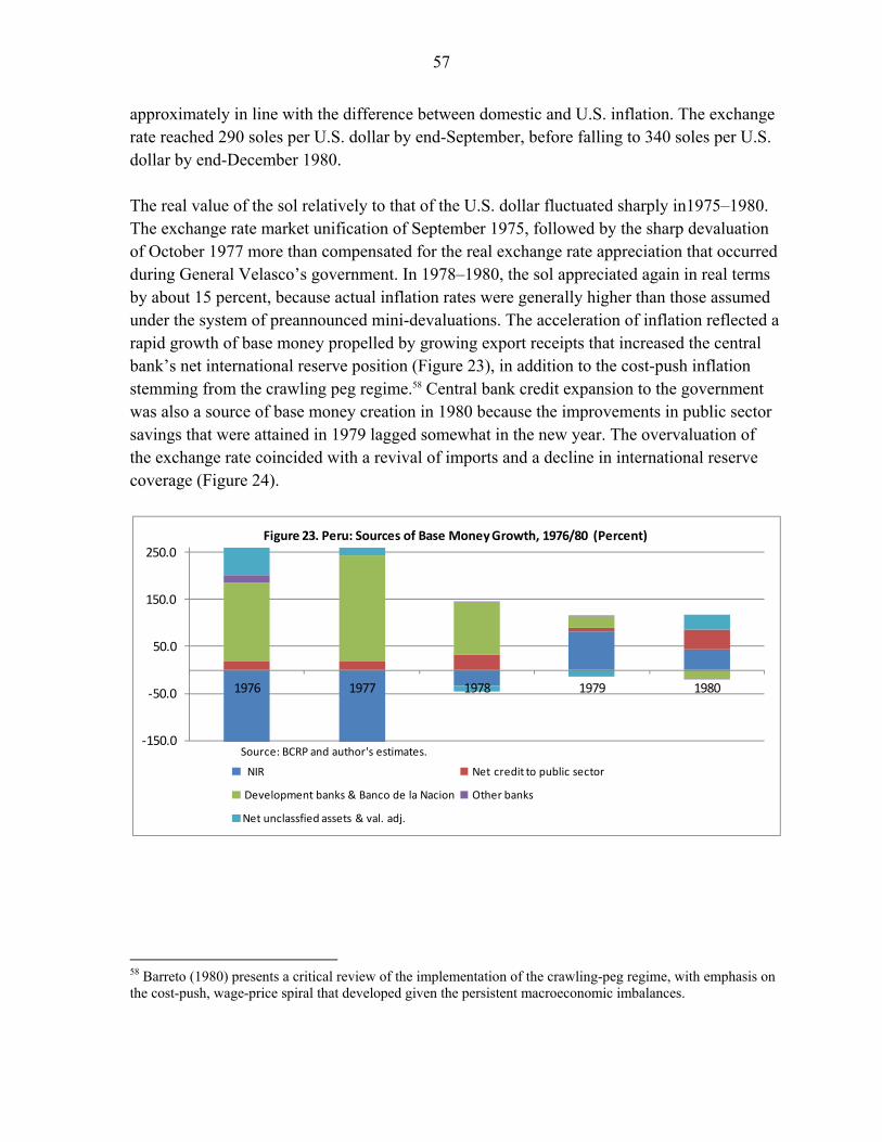
57

approximately in line with the difference between domestic and U.S. inflation. The exchange rate reached 290 soles per U.S. dollar by end-September, before falling to 340 soles per U.S. dollar by end-December 1980. The real value of the sol relatively to that of the U.S. dollar fluctuated sharply in1975–1980. The exchange rate market unification of September 1975, followed by the sharp devaluation of October 1977 more than compensated for the real exchange rate appreciation that occurred during General Velasco’s government. In 1978–1980, the sol appreciated again in real terms by about 15 percent, because actual inflation rates were generally higher than those assumed under the system of preannounced mini-devaluations. The acceleration of inflation reflected a rapid growth of base money propelled by growing export receipts that increased the central bank’s net international reserve position (Figure 23), in addition to the cost-push inflation stemming from the crawling peg regime.58 Central bank credit expansion to the government was also a source of base money creation in 1980 because the improvements in public sector savings that were attained in 1979 lagged somewhat in the new year. The overvaluation of the exchange rate coincided with a revival of imports and a decline in international reserve coverage (Figure 24).

58 Barreto (1980) presents a critical review of the implementation of the crawling-peg regime, with emphasis on the cost-push, wage-price spiral that developed given the persistent macroeconomic imbalances.

-150.0

-50.0

50.0

150.0

250.0

1976 1977 1978 1979 1980

Figure 23. Peru: Sources of Base Money Growth, 1976/80 (Percent)

NIR Net credit to public sector

Development banks & Banco de la Nacion Other banks

Net unclassfied assets & val. adj.

Source: BCRP and author's estimates.

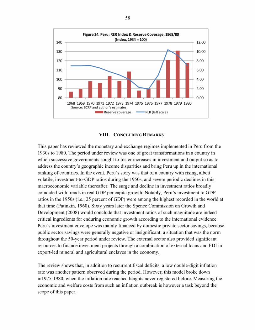
58

VIII. CONCLUDING REMARKS

This paper has reviewed the monetary and exchange regimes implemented in Peru from the 1930s to 1980. The period under review was one of great transformations in a country in which successive governments sought to foster increases in investment and output so as to address the country’s geographic income disparities and bring Peru up in the international ranking of countries. In the event, Peru’s story was that of a country with rising, albeit volatile, investment-to-GDP ratios during the 1950s, and severe periodic declines in this macroeconomic variable thereafter. The surge and decline in investment ratios broadly coincided with trends in real GDP per capita growth. Notably, Peru’s investment to GDP ratios in the 1950s (i.e., 25 percent of GDP) were among the highest recorded in the world at that time (Patinkin, 1960). Sixty years later the Spence Commission on Growth and Development (2008) would conclude that investment ratios of such magnitude are indeed critical ingredients for enduring economic growth according to the international evidence. Peru’s investment envelope was mainly financed by domestic private sector savings, because public sector savings were generally negative or insignificant: a situation that was the norm throughout the 50-year period under review. The external sector also provided significant resources to finance investment projects through a combination of external loans and FDI in export-led mineral and agricultural enclaves in the economy. The review shows that, in addition to recurrent fiscal deficits, a low double-digit inflation rate was another pattern observed during the period. However, this model broke down in1975-1980, when the inflation rate reached heights never registered before. Measuring the economic and welfare costs from such an inflation outbreak is however a task beyond the scope of this paper.

0.00

2.00

4.00

6.00

8.00

10.00

12.00

80

90

100

110

120

130

140

1968 1969 1970 1971 1972 1973 1974 1975 1976 1977 1978 1979 1980

Figure 24. Peru: RER Index & Reserve Coverage, 1968/80 (Index, 1934 = 100)

Reserve coverage RER (left scale)

Source: BCRP and author's estimates.

59

The relatively small size and openness of the Peruvian economy called for a strong partnership with the rest of the world in terms of export markets and technical knowledge at all times. Leaders, including military caudillos like Sanchez Cerro, Odría, Velasco and Morales Bermudez, reached out to international forums like the Kemmerer mission, the Klein mission report, and the Bretton Woods institutions (such as the IMF and the World Bank) to support their governments’ policies in times of economic stress. The ultimate policy decisions however, rested with the Peruvian authorities, who, at times, chose to disagree with their foreign advisers. Examples include the timely suspension of the currency convertibility proposed by the Kemmerer mission (1931) given the balance of payments deficits, and the decision by the Central Reserve Bank to terminate the parity for the sol against the U.S. dollar in late-1949 and never to resume it despite the prevailing Bretton Woods system of fixed exchange rates that was in place until the early-1970s. The dynamics of the export sector and the strength of the central bank’s external position were always relevant. During export booms and periods of rising FDI, the policy challenge was how to contain the growth of monetary aggregates and inflation. Controlling inflationary expectations was critical for containing the appreciation of the real exchange rate and its negative impact on international reserves. When the external environment was bleak and/or uncertain, the challenge was how to arrest excessive growth of imports and also protect the international reserve position. Much intellectual power in policy analysis and design was needed at all times, with the Central Reserve Bank being consistently a readily available source for technical advice and analytical rigor for the government. At times, the central bank went beyond the call of duty for a monetary institution, immersing its Economic Studies Department in the preparation of Peru’s first comprehensive economic development program (Banco Central de Reserva del Perú, 1961) that identified long-run economic issues and challenges for policymakers of those times. In terms of hard numbers, the data show that nominal exchange rates were not that flexible during the half-century covered by this paper, rather, there was a sequence of broadly stable nominal exchange rates episodes followed by discrete upward adjustments (devaluations) of the national currency. Only the 1930s and 1950s saw enhanced nominal exchange rate flexibility, with the 1950s being considered by some scholars a unique experiment with floating exchange rates in a developing country (Edwards, 1983; Hamann and Savastano, 1985; and Tsiang, 1956). The mini-devaluations of 1978–80 also enhanced exchange rate flexibility, although the exchange rate system was not that of a float, but rather one of adjustable fixed rates in line with the actual and/or expected rate of domestic inflation. While the nominal exchange rate stability supported, in principle, lower domestic inflation than otherwise, it critically influenced trends of the real effective exchange rate (i.e., the

60

nominal exchange rate adjusted by Peru’s inflation differential with the U.S.) that affected overall macroeconomic conditions. Periods of nominal exchange rate stability (i.e., 1940–1948, 1960–67, 1970–75) led to a significant overvaluation of the domestic currency that resulted in rapid growth of commodity imports and domestic demand, albeit accompanied by growing external current account deficits and dwindling central bank international reserves. By contrast, the adjustments in the level of the nominal exchange rate, which were generally complemented by tight financial policies, led to slowing import growth and overall economic activity, as well as improvements in the balance of payments. The exchange rate stability or flexibility registered at different times reflected neither a rigid adherence to a system of fixed parities against the U.S. dollar nor a system of complete emphasis on monetary aggregates without concern for the exchange rate. Rather, both periods were hybrid implementations of textbook cases of fixed and floating exchange rate regimes. In either regime, the monetary authorities erred on the side of delivering exchange rate stability even at the cost of introducing market distortions (i.e., exchange and trade restrictions) and/or incurring heavy losses in international reserves. For example, the exchange rate stability of the 1940s, during the Second World War, led to the introduction of exchange and trade controls to force a quick adaptation of imports to export receipts. Also, the Peruvian experience of floating exchange rates of the 1950s delivered remarkable “stability” of the floating exchange rate for a number of years (especially in 1954–57) that was achieved at the cost of heavy losses in reserves. This historical review also shows that the level of the real exchange rate and the investment-to-GDP ratios registered between late-1949 and 1962 were the highest ever recorded for Peru. No period between 1930 and 1980 had a more competitive real exchange rate and higher investment ratios than those registered in that thirteen year episode. The years1938–1944 had some resemblance with the 1949–1962 episode in terms of the levels of the real exchange rate, but domestic investment ratios and economic growth rates were more limited. Also, the time between the rise in the real exchange rate level and the return to earlier exchange rate levels was only 6 years, compared with a 13-year interval registered in the 1950s. During the military government of 1975–1980, there was a temporary recovery in the real exchange rate from the lows recorded at the end of the Velasco’s administration, but the period was short-lived (1975–78) and investment and economic activity were significantly depressed. High inflation in 1979–80 lowered the real exchange rate, thus putting renewed pressure on export competitiveness and triggering import growth. The historical review has traced the evolution of monetary policy through the years. We find numerous moments in 1930–1980, in which the monetary authority adjusted banks’ reserve requirements to complement fiscal consolidation efforts underway and to arrest the growth of credit and support a restoration of the international reserve position. Interestingly, a genesis

61

of the modern sterilization mechanism used by most central banks today, including the Central Reserve Bank of Peru, appeared only during the Velasco administration in which treasury bills were used to mop up banks’ liquidity. Unfortunately, the liquidity subtracted from the economy was injected again through a non-transparent system of quasi-fiscal operations that financed the development banks and, ultimately, the central government deficit. Another casualty during the military regime of 1968–1980 was the apparent loss of central bank independence, which had been a hard-won process attained only in 1961 with the issuance of a new Central Bank Law. The establishment of the Monetary Policy Council which was superior in authority to the Central Reserve Bank and was in charge of determining Peru’s credit, monetary, and exchange rate policy did not bear well in terms of best international practices, although the data, in terms of the components of base money creation, and the testimony recorded in the central bank minutes suggest a high degree of fiscal dominance over monetary decisions in place both before and after the military regime. The review finishes in 1980. This paper hopefully fills a gap in the understanding of the monetary policy in Peru. Yet, the years 1980–85 were a dramatic period for Peru, in which output first stagnated during 1980–82 and then dropped by 16 percent over 15 months, while inflation doubled to 120 percent in early 1983, and doubled again to 250 percent in early 1985. Policymakers faced challenges never seen before in Peru during those years. The task of recording and thoroughly analyzing those events by economic practitioners and historians thus remains and merits our attention. In the words of César Vallejo we could confidently say: “Hay, compañeros, muchísimo por hacer” (Vargas Llosa (2010)).

62

IX. SELECTED BIBLIOGRAPHY

Banco Central de Reserva del Perú (1961), Plan Nacional de Desarrollo Económico y Social del Perú, 1962–1971, Tomo 1, 500 pages Banco Central de Reserva del Perú (1999), El Banco Central: Su Historia y la Economía del Perú 1821–1992, three volumes, Lima, Perú. Banco Central de Reserva del Perú (n.d.), La Misión Kemmerer en el Perú, two volumes, impresion Ausonia SA., Lima, Peru. Bardella, Gianfranco (1989), Un Siglo en la Vida Económica del Perú: 1889–1989, Banco de Crédito del Perú, Lima, May, 632 pages. Barreto, Emilio G. (1936), El Valor Adquisitivo de la Moneda: Otras Cuestiones Monetario-Bancarias, Editorial Lumen, Lima, Peru, 176 pages. Barreto, Emilio G. (1943), “La Política Monetaria del Perú de 1900 a 1940,” in El Sistema Monetario del Perú, by Bruno Moll and Emilio G. Barreto (1943), Revista de Economía y Estadística, Año IV, No.3, Imprenta de la Universidad de Córdoba, Republica Argentina. Barreto, Emilio G. (1972), “Las Reformas Financieras del Perú de 1968 a 1971,” Conferencia de prensa del doctor Emilio G. Barreto, mimeo, Lima, Peru. Barreto, Emilio G. (1980), Perú: Los Desarrollos Económicos y Financieros: 1970–1980, Fondo Editorial del Banco Central de Reserva del Perú, Imprenta B.C.R.P., September, 370 pages. Basadre, Jorge (2003), “La Estructura Económica,” in Ernesto Yepes del Castillo, Memoria y Destino del Perú: Jorge Basadre, Textos Esenciales, Fondo Editorial del Congreso del Perú, Lima, pages 443–494. Boloña, Carlos (1981), Tariff Policies in Peru, 1880–1980, Ph.D. dissertation, Oxford University. Contreras, Carlos and Marcos Cueto (2004), Historia del Perú Contemporáneo: Desde las luchas por la Independencia hasta el presente, Pontificia Universidad Católica del Perú, Universidad del Pacifico, Instituto de Estudios Peruanos, 422 pages, Talleres Gráficos de Tarea Asociación Grafica Educativa, Lima, Peru.

63

Corden, Max and Peter Neary (1982), "Booming Sector and De-industrialisation in a Small Open Economy", The Economic Journal (December): pages 825–848. Edwards, Sebastian (1983), “Floating Exchange Rates in Less-Developed Countries: A Monetary Analysis of the Peruvian Experience, 1950–54,” Journal of Money, Credit and Banking, vol. 15, No.1, February, pages 73–81. Ferrero, Rómulo (1963), “El Desarrollo de la Economía Nacional en los Últimos Veinticinco Años” en José Pareja y Paz Soldán, Visión del Perú en el Siglo XX, Librería Studium S.A., Lima. Guevara Ruiz, Guillermo (1999), “Política Monetaria del Banco Central: Una Perspectiva Histórica,” Revista Estudios Económicos 5, Banco Central de Reserve del Perú, available on the central bank’s website. Hamann, Alfonso Javier and Miguel Aldo, Savastano (1985), El Enfoque Monetario de la Determinación del Tipo de Cambio en los Países en Vías de Desarrollo: Un Análisis de la Experiencia Peruana (1949–1954), Tesina presentada para la obtención del grado académico de bachiller en economía, Universidad del Pacifico, Facultad de Economía, 155 pages. Haya de la Torre, Victor Raúl (1936), El Antiimperialismo y el Apra, Chile. Hayn, Rolf (1955) “Peruvian Monetary and Foreign-Exchange Policy, 1940–1945,” in Inter-American Economic Affairs, volume VIII, No.4, Spring, pages 23–42. Hayn, Rolf (1957) “Peruvian Exchange Controls: 1945–1948,” in Inter-American Economic Affairs, volume X, No.4, Spring, pages 47–70. Hernández, Marco Antonio (2008), The State, Capital, and Economic Statecraft: The Political Economy of State-Business Relations in Peru and Chile, Ph.D. dissertation, Oxford University. International Monetary Fund (IMF) Archives: Initial Par Values – Peru, EBD/46/130 of 11/25/1946.

Exchange Market in Peru, SM/47/43 of 1/29/1947.

Supplementary Material on Peru in connection with the Preliminary Report of the Fund’s Representatives, SM/48/188 of 2/21/1948.

64

Report to Peru, SM/48/212 of 4/2/1948.

Report of Fund Representative on Visit to Peru, SM/48/293 of 12/1/1948.

The Peruvian Exchange Proposals, SM/48/268 of 8/31/1948.

Peru: Recent Economic Developments, SM/49/375 of 7/7/1949.

1955 Consultations – Peru, SM/55/46 of 7/18/1955.

1956 Consultations and Use of the Fund’s Resources– Peru, SM/57/4 of 1/18/1957.

1957 Consultations – Peru, SM/57/99 of 12/6/1957. Request for Stand-By Arrangement – Peru, EBS/59/13 of 2/24/1959. Peru – Unification of Exchange Markets, SM/60/40 of 5/25/1960.

Peru – 1960 Consultations, SM/61/9 of 2/14/1961.

Peru – Request for Stand-By Arrangement, EBS/62/17 of 2/15/1962.

EBS/63/24, Peru – Request for Stand-By Arrangement, 2/14/1963.

Peru – 1963 Article VIII Consultations, SM/64/19 of 2/14/1964.

Peru – 1964 Article VIII Consultations, SM/65/26 of 3/25/1965.

Peru – Request for Stand-By Arrangement, EBS/66/73 of 3/16/1966.

Peru – Request for Stand-By Arrangement, EBS/67/162 of 8/4/1967.

Peru – Request for Stand-By Arrangement, EBS/68/240 of 9/9/1968.

Peru – 1968 Article VIII Consultation, SM/68/153 of 10/9/1968.

Supplement 1, Peru – Request for Stand-By Arrangement, EBS/68/240 of 11/1/1968.

Peru – Use of Fund’s Resources, EBS/72/178 of 6/1/1972.

Supplement 1, Peru – Purchase Transaction, EBS/72/178 of 6/14/1972.

Peru – Use of Fund Resources – Compensatory Financing, EBS/76/173 of 4/16/1976.

Peru – Recent Economic Developments, SM/72/206 of 8/29/1972.

65

Peru – Request for Stand-By Arrangement, EBS/77/393 of 10/28/1977. Peru – Request for Stand-By Arrangement, EBS/78/447 of 10/18/1978. Peru – Use of Fund Resources – Compensatory Financing Facility, EBS/78/464 of 8/25/1978. Peru – Request for Stand-By Arrangement, EBS/79/360 of 6/28/1979. Par Value-Peru, EBM No. 626 of 12/18/1950.

1952 Consultation –Peru, EBM/52/69.

Use of Fund’s Resources – Peru, EBM/54/6 of 2/12/54. 1953 Consultations and Use of the Fund’s Resources – Peru, EBM/54/7 of 2/17/1954. Use of Fund’s Resources – Peru, EBM/55/9 of 2/16/1955. 1955 Consultations – Peru, EBM/55/49 of 7/28/1955. Use of the Fund’s Resources – Peru, EBM/56/10 of 2/10/1956. Peru – 1956 Consultations, EBM/57/6 of 2/6/1957. 1957 Consultations – Peru, EBM/57/61 of 12/30/1957. Use of Fund’s Resources – Stand-By Arrangement with Peru, EBM/58/45 of 9/12/1958.

Use of the Fund’s Resources – Stand –by Arrangement with Peru, EBM/59/3 of 2/11/1959. Peru – 1958 Consultations and Use of Fund’s Resources, EBM/59/6 of 2/27/1959. Peru – Acceptance of Obligations of Article VIII, Sections 2, 3, and 4, EBM/61/4 of 2/8/1961.

Peru – 1959 Consultations and Use of the Fund’s Resources, EBM/60/7 of 2/29/1960.

Peru – 1961 Article VIII Consultations and Stand-By Arrangement, EBM/62/8 of 2/26/1962.

66

Peru – 1962 Article VIII Consultations and Stand-By Arrangement, EBM/63/7 of 2/25/1963.

Peru – 1963 Article VIII Consultations and Stand-By Arrangement, EBM/64/11 of 2/28/1964.

Peru – 1964 Article VIII Consultations and Stand-By Arrangement, EBM/65/1965 of 4/7/1965.

Peru – 1965 Article VIII Consultations and Stand-By Arrangement, EBM/66/21 of 3/30/1966.

Peru – Modification of Stand-By Arrangement, EBM/66/42 of 6/15/1966.

Instituto Nacional de Planificación (1979), Cuentas Nacionales del Perú: 1950–1978, Oficina Nacional de Estadística (ONE), Dirección de Cuentas Nacionales, May, 160 pages. Kalin, Irving (1953), “Thriving Peru: Its Switch from Bust to Boom Shows What a Free Economy Can Do,” The Wall Street Journal, February 11, 1953. Klein, Julius (1949), “Reforma Monetaria en el Perú,” El Trimestre Económico, 16, Fondo de Cultura Económica, México, December, pages 600-619. Kuczynski, Pedro Pablo (1977), Peruvian Democracy under Economic Stress: An Account of the Belaúnde Administration, 1963–1968, Princeton University Press, Princeton, New Jersey, xiii + 314 pages. Kurbs, Friedrich (1939), “Introducción,” Extracto Estadístico del Perú, Dirección Nacional de Estadística, Imprenta Americana, Lima, Perú, pages I-CXXIII. Little, Arthur D. (1960), Programa de Desarrollo Industrial y Regional para el Perú, Lima. Lovasy, Gertrud (1961), “Note on Exchange Depreciation and Export Developments in Peru,” International Monetary Fund, DM/61/18, Research and Statistics Department, Washington D.C., June, 12 pages. Mariátegui, José Carlos (1928), 7 Ensayos de Interpretación de la Realidad Peruana, Lima, Perú, Biblioteca Amauta, 352 pages. Ocampo, José Antonio (1988), “Crisis Mundial y Cambio Estructural (1929–1945),” in José Antonio Ocampo (compilador), Historia Económica de Colombia, Siglo Veintiuno Editores, pages 206–242.

67

Patinkin, Don (1960), The Israel Economy: The First Decade, The Falk Project for Economic Research in Israel, Jerusalem, December, 160 pages. Polak, Jacques J. (1948), “Depreciation to meet a Situation of Overinvestment,” in Frankel, Jacob A. and Morris Goldstein (1991), editors, International Financial Policy—Essays in Honor of Jacques J. Polak, Washington: International Monetary Fund and De Nederlandsche Bank, pages 46–57. Polak, Jacques J. (1957), “Monetary Analysis of Income Formation and Payments Problems”, in International Monetary Fund (1977), The Monetary Approach to the Balance of Payments, Washington D.C. pages 15–64. Polak, Jacques J. (1997), “The IMF Monetary Model at Forty,” International Monetary Fund, Working Paper, WP/97/49, April, 20 pages. Quiroz, Alfonso W. (1986), Financial Institutions in Peruvian Export Economy and Society, 1884–1930, Ph.D. dissertation, Columbia University. Quiroz, Alfonso W. (1991), “Financial Development in Peru under Agrarian Export Influence, 1884–1950,” The Americas, Vol.47, No.4, April, pp. 447–476. Quiroz, Alfonso W. (2011), “Mirando Hacia Adentro, 1930–1960: El Proceso Económico” in Marcos Cueto and Carlos Contreras, editores, América Latina en la Historia Contemporánea: Mirando Hacia Adentro, Madrid: Mapfre Editores, forthcoming. Roemer, Michael (1970), Fishing for Growth: Export-led Development in Peru, 1950–1967, Harvard University Press, Cambridge, Massachusetts, 208 pages. Rojas, Jorge (1993), “El Perú hasta 1960: Políticas Liberales en una Economía Abierta,” mimeo, Serie Documentos de Trabajo, No. 109, March, 51 pages. Seminario, Bruno and Arlette Beltrán (1998), Crecimiento Económico en el Perú: 1896-1995, Nuevas Evidencias Estadísticas, Lima, Centro de Investigación de la Universidad del Pacifico. Spence Commission on Growth and Development (2008), The Growth Report: Strategies for Sustained Growth and Inclusive Development, The International Bank for Reconstruction and Development/The World Bank, Washington D.C., 180 pages.

68

Thorp, Rosemary and Geoffrey Bertram (1978), Peru 1980–1977: Growth and Policy in an Open Economy, Columbia University Press, New York, xv + 478 pages. Triffin, Robert (1946), “Esbozo General de un Análisis de las Series Estadísticas Monetarias y Bancarias de América Latina sobre Bases Uniformes y Comparables,” in Memoria: Primera Reunión de Técnicos sobre Problemas de la Banca Central del Continente Americano, Mexico City: Banco de México, pp. 410–430. Tsiang, S. C. (1956), “An Experiment with a Flexible Exchange Rate System: The Case of Peru 1950–1954,” International Monetary Fund, DM/56/22, Research and Statistics Department, Washington D.C., July, 30 pages, published in International Monetary Fund Staff Papers, 5, November 1957, pages 449–476. Vargas Llosa, Mario (2010), “Elogio a la Lectura y la Ficción: Discurso del Nobel,” Nobel Lecture, Stockholm, December 10, 2010. Webb, Richard (1987), Country Study No.8: PERU, Stabilization and Adjustment Programmes and Policies, World Institute for Development Economics Research of the United Nations University, WIDER Publications, 44 pages, Helsinki, Finland. Webb, Richard (2009), “Emilio G. Barreto,” El Comercio, 16 de Marzo. Yepes, Ernesto (1992), La Modernización en el Perú del Siglo XX: Ilusión y Realidad, Mosca Azul Editores, Economía y Política, 92 pages.