Embed Size (px)
Citation preview
On Credible Monetary Policies with Model Uncertainty∗
Anna Orlik † Ignacio Presno ‡
June 3, 2013
Abstract
This paper studies the design of optimal time-consistent monetary policy in an economy
where the planner trusts his own model, while a representative household uses a set of
alternative probability distributions governing the evolution of the exogenous state of the
economy.
In such environments, unlike in the original studies of time-consistent monetary policy,
management of households’ expectations becomes an active channel of optimal policymak-
ing per se; a feature that our paternalistic government seeks to exploit.
We adapt recursive methods in the spirit of Abreu et al. (1990) as well as computational
algorithms based on Judd et al. (2003) to fully characterize the equilibrium outcomes for a
class of policy games between the government and a representative household who distrusts
the model used by the government.
1 Introduction
Undoubtedly, inflation expectations of the public influence greatly actual inflation, and, there-
fore, a central bank’s ability to achieve price stability. But what do we mean precisely by the
”state of inflation expectations”? And, most importantly, what role does monetary policy
play in shaping or managing inflation expectations1?
∗We are especially grateful to Thomas J. Sargent for his support and encouragement. We thank David
Backus, Roberto Chang, Timothy Cogley, Stanley Zin and seminar participants at Bank of England, Board of
Governors of the Federal Reserve System, Carnegie Mellon University, UPF-CREI, and Federal Reserve Bank
of San Francisco, for helpful comments.†Address: Board of Governors of the Federal Reserve System, 20th Street and Constitution Avenue NW
Washington, DC 20551, Email: [email protected].‡Address: Federal Reserve Bank of Boston, 600 Atlantic Avenue Boston, MA 02110, Email: igna-
[email protected] questions are subject of Bernanke (2007).
1
In this paper, the management of private beliefs by a central banker becomes an integral
part of the theory of optimal monetary policy making.
In our modeled economy, which we construct in the tradition of monetary models of Calvo
(1978) and Chang (1998), a representative household derives utility from consumption and
real money holdings. The government uses the newly printed money to finance transfers or
taxes to households. Taxes and transfers are distortionary. The only source of uncertainty
in this economy is a shocks that affects the degree of tax distortions through its influence on
households’ income.
At the heart of this paper lies the assumption that the government has a single approx-
imating model that describes the evolution of the underlying state of the economy while a
representative household fears it might be misspecified. To confront that concern, a rep-
resentative household contemplates a set of nearby probability distributions governing the
evolution of the underlying shock and seeks decision rules that would work well across these
models. The household assesses the performance of a given decision rule by computing the
expected utility under the worst-case density within the set.
The fact that private agents seem unable to assign a unique probability distribution to
alternative outcomes has been demonstrated in Ellsberg (1961) and similar experimental
studies2. Moreover, lack of confidence in the models seems to have become apparent during
the recent financial crisis3. Below we present the quote from Bernanke (2010)
”Most fundamentally, and perhaps most challenging for researchers, the crisis should motivate
economists to think further about modeling human behavior. Most economic researchers continue
to work within the classical paradigm that assumes rational, self-interested behavior and the
maximization of ”expected utility” (...). An important assumption of that framework is that,
in making decisions under uncertainty, economic agents can assign meaningful probabilities to
alternative outcomes. However, during the worst phase of the financial crisis, many economic
actors–including investors, employers, and consumers– metaphorically threw up their hands and
admitted that, given the extreme and, in some ways, unprecedented nature of the crisis, they did
not know what they did not know.”
The government in our model follows the above advice; he recognizes that households are
not able or willing to assign a unique probability distribution to alternative realizations of
the stochastic state of the economy. The government wants to design optimal policy that
explicitly accounts for the fact that households’ allocation rules are influenced by how they
form their beliefs in light of model uncertainty.
We characterize optimal policy under two timing protocols for government’s choices. First,
we work under the assumption that the government can commit at time zero to a policy speci-
fying its actions for all current and future dates and states of nature. Under this assumption, a
2See, e.g.Halevy (2007).3See e.g. Caballero and Krishnamurthy (1998), and Uhlig (2010).
2
government chooses at time zero the best competitive equilibrium from the set of competitive
equilibria with model uncertainty, i.e. one that maximizes the expected households’ lifetime
utility but under its own unique belief. We will refer to such a government as paternalistic
Ramsey planner.
The competitive equilibrium conditions in our context are represented by households’ Euler
equations and an exponential twisting formula for the beliefs’ distortions. Using insights of
Kydland and Prescott (1980), we express the set of competitive equilibria in a recursive way by
introducing an adequate pair of state variables. We need first to keep track of the equilibrium
(adjusted) marginal utilities to guarantee that the Euler equations are satisfied after each
history. Our second state variable is households’ lifetime utility. This variable is needed
to express the equilibrium beliefs’ distortions in the context of model uncertainty. These
two variables summarize all the relevant information about future policies and allocations
for households’ decision making when the government has the ability to commit. Through
the dynamics of the promised marginal utility and households’ continuation value, which the
government has to be able to deliver in equilibrium, the solution to the government’s problem
under commitment, the Ramsey plan, exhibits history dependence.
Once we abstract from the assumption that the government has the power to commit,
and, instead, chooses sequentially, time inconsistency problem may arise, as first noted by
Kydland and Prescott (1977) and Calvo (1978). The government will adhere to a plan only
if it is optimal after any realized history. Thereofre, we need to check whether the optimal
policies derived by our paternalistic Ramsey planner are time consistent, and, more generally,
to characterize what we call the set of sustainable plans with model uncertainty4. This latter
notion should be thought of as an extension of Chari and Kehoe (1990).
Using the government’s continuation value as an additional third state variable, in order
to keep track of an appropriate incentive constraint for the government, we provide a complete
recursive formulation of a sustainable plan under model uncertainty. In this formulation, a
new source of history-dependence arises and it is given by the restrictions that the system of
households’ expectations imposes on government’s policy actions in equilibrium.
This paper constitutes the first attempt to characterize the set of all time-consistent out-
comes when agents exhibit any form of uncertainty aversion in an infinite-horizon model.
This particular feature of our environment provides the opportunities to the government to
influence households’ beliefs about exogenous variables through their expectations of future
4The notion of a sustainable plan inherits sequential rationality on the government’s side, jointly with
the fact that households always respond to government actions by choosing from competitive equilibrium
allocations.
3
policies, which have to be confirmed in equilibrium. The management of households’ beliefs
becomes an active channel of policy-making as the government will try to optimally exploit
the dependence of households’ equilibrium beliefs on the path of future policies.
Characterizing time-consistent outcomes is a challenging task. This is because any time
consistent solution must include a description of government and market behavior such that
the continuation of such behavior after any history is a competitive equilibrium and it is
optimal for the government to follow that policy. In this paper, we use insights from the
work by Abreu et al. (1990), Chang (1998), Phelan and Stacchetti (2001) to compute the sets
of equilibrium payoffs as the largest fixed point of a particular operator which we construct
and describe in detail. Also, we adapt algorithms in the spirit of Judd et al. (2003) based
on hyperplane approximation methods that let us compute the equilibrium values sets in
question. The characterization of the entire set of sustainable equilibrium values facilitates
the examination of practical policy questions. Our numerical examples suggest that policies
that account for the fact that households contemplate a set of probability distributions may
lead to better outcomes in terms of welfare.
Although in this paper we restrict attention to the type of models of monetary policy-
making which can be cast in the spirit of Calvo (1978), hopefully it will become clear that
our approach could be applicable to many repeated or dynamic games between a government
and a representative household who distrusts the model used by the government.
To our knowledge, there are two papers that try to explore the role of policy maker
in managing households’ expectations in the presence of model uncertainty. Karantounias
et al. (2009) study the optimal fiscal policy problem of Lucas and Stokey (1983) but in an
environment where a representative household distrusts the model governing the evolution of
exogenous government expenditure. The authors apply techniques of Marcet and Marimon
(2009) to characterize the optimal policies when the government is assumed to have the power
to commit. Woodford (2003) discusses the optimal monetary policy under commitment in
an economy where both the government and the private sector fully trust their own models,
but the government distrusts its knowledge of the private sector’s beliefs about prices. With
respect to both of these paper, our study can be seen as providing arguments to question
the government’s ability to commit which go beyond the usual reasons for potential time
inconsistency of government’s policies and that have to do with planner’s ability to influence
the equilibrium system of beliefs of the private agents.
The remainder of this paper is organized as follows. Section 2 sets up the model and out-
lines the assumptions made. In Section 3 we introduce the notion of competitive equilibrium
with model uncertainty. In Section 4 we discuss the recursive formulation of the Ramsey
4
problem for the paternalistic government. Section 5 contains the discussion of sustainable
plans with model uncertainty. In Section 6 we describe the computational algorithms we have
implemented to determine the set of all the equilibrium values to the government and to the
representative household, and promised marginal utilities. Also, we present numerical results.
Section 7 briefly discusses an alternative hypothesis with both the government and households
using, possibly distinct, sets of models. Finally, Section 8 concludes.
2 Benchmark Model
The economy is populated by two infinitely-lived agents: a representative household (with
her evil alter ego, which represents her fears about model misspecification) and a government.
The household and the government interact with each other at discrete dates indexed as
t = 0, 1, ....
At the beginning of each period, the economy is hit by an exogenous shock that affects the
final output level. While the government fully trusts the probability distribution for the shock,
the representative household fears that it is misspecified. In turn, she contemplates a set of
alternative probability distributions to be endogenously determined, and seeks decision rules
that perform well over this set of distributions. Given her doubts on which model actually
governs the evolution of the shock, the household designs decision rules that guarantee lower
bounds on expected utility level under any of the distributions.
Let (Ω,F ,Pr) be the underlying probability space. Let the exogenous shock be given by
st, where s0 ∈ S is given (there is no uncertainty at time 0) and st : Ω→ S for all t > 0. The
set S the shock can take values from is assumed to be finite with cardinality S. We assume
that st follows a Markov process for all t > 0, with transition density given by π (st+1|st).Throughout the paper we will refer to the conditional density π (st+1|st) as the approxi-
mating model. Let st ≡ (s0, s1, ..., st) ∈ S×S× ...×S ≡ St+1 be the history of the realizations
of the shock up to t. Finally, we denote by St ≡ F(st)
the sigma-algebra generated by the
history st.
2.1 Representative Household’s Problem and her Fears about Model Mis-
specification
Households in this economy derive utility from consumption of a single good, c(st), and real
money balances, m(st). The households’ period payoff is given by u(ct(st))
+ v(mt
(st)),
where the utility components u and v satisfy the following assumptions
5
[A1] u : R+ → R is twice continuously differentiable, strictly increasing, and strictly
concave
[A2] v : R+ → R is twice continuously differentiable, and strictly concave
[A3] limc→0 u′ (c) = limm→0 v
′ (m) = +∞
[A4] ∃m < +∞ such that v′ (m) = 0
The assumptions [A1]-[A3] are standard. Assumption [A4] establishes a satiation level for
real money balances.
In this paper we model the representative household as being uncertainty-averse. While
the government fully trusts the approximating model π(st), the household distrusts it. For
this reason, she surrounds it with a set of alternative distributions π(st)
that are statistical
perturbations of the approximating model, and seeks decision rules that perform well across
these distributions. We assume that these alternative distributions, π (st), are absolutely
continuous with respect to π (st), i.e. π (st) = 0⇒ π(st)
= 0, ∀st ∈ St+1.
By invoking Radon-Nikodym theorem we can express any of these alternative distorted
distributions using a nonnegative St-measurable function given by
Dt
(st)
=
π(st)π(st) if π
(st)> 0
1 if π(st)
= 0
which is a martingale with respect to π(st), i.e.
∑st+1
π (st+1|st)Dt+1
(st+1
)= Dt
(st). We can
also define the conditional likelihood ratio as dt+1
(st+1|st
)≡ Dt+1(st,st+1)
Dt(st)for Dt
(st)> 0.
Notice that in case Dt
(st)> 0 it follows that
dt+1
(st+1|st
)=
π(st+1|st)π(st+1|st) if π
(st+1
)> 0
1 if π(st+1
)= 0
and that the expectation of the conditional likelihood ratio under the approximating model
is always equal to 1, i.e.∑st+1
π(st+1|st
)dt+1(st+1|st) = 1.
To express the concerns about model misspecification, we follow Hansen and Sargent
(2008) and endow the household with multiplier preferences. Under this assumption, the set
of alternative distributions over which the household evaluates the expected utility of a given
decision rule is given by an entropy ball endogenously determined. We can then think of the
household as playing a zero-sum game against her evil alter ego, who is a fictitious agent that
represents her fears about model misspecification. The evil alter ego will be distorting the
6
expectations of continuation outcomes in order to minimize the household’s lifetime utility.
He will do it by selecting a worst-case distorted model π(st), or equivalently, a sequence of
probability distortionsDt
(st), dt+1
(st+1|st
)∞t=0
.
The representative household, thus, ranks consumption and money balances plans accord-
ing to
V H = maxct(st),mt(st)
minDt(st),dt+1(st+1)
∞∑t=0
βt∑st
π(st)Dt(st)[u(ct(st))
+ v(mt
(st))]
+θβ∑st+1
π(st+1|st)dt+1(st+1|st) log dt+1(st+1|st)
(1)
Dt+1(st+1) = dt+1(st+1|st)Dt(st) (2)∑
st+1
π(st+1|st)dt+1(st+1|st) = 1 (3)
where mt ≡ qtMt is the real money balances, Mt is the money holdings at the end of period
t, qt is the value of money in terms of the consumption good (that is, the reciprocal of the
price level), and θ ∈ (θ,+∞] is a penalty parameter that controls the degree of concern about
model misspecification. Through the last term, the entropy term, the evil alter ego is being
penalized whenever he selects a distorted model that differs from the approximating one.
Note that the higher the value of θ, the more the evil alter ego is being punished. If we let
θ → +∞ the probability distortions to the approximating model vanish, the household and
the government share the same beliefs, and expression (1) collapses to the standard expected
utility.
Conditions (2) and (3) discipline the choices of the evil alter ego. (2) defines recursively the
likelihood ratio Dt. Condition (3) guarantees that every distorted probability is a well-defined
probability measure.
The minimization problem of the evil alter ego yields lower bounds (in terms of expected
utility) on the performance of any decision rule of the household. The probability distortion
d(st+1|st) that solves such minimization problem satisfies the following exponential twisting
formula
d(st+1|st) =exp
(−V H(st+1)
θ
)∑
st+1∈S π(st+1|st) exp(−V H(st+1)
θ
) (4)
where V H(st+1) is the t+1−equilibrium value for the household. (4) shows how the evil alter
ego pessimistically twists the households’ beliefs by assigning high probability distortions to
the states st+1 associated with low utility for the household, and low probability distortions
to the high-utility states. See the Appendix A.1 for the derivation of (4). Notice from (4)
7
that to express the optimal belief distortions, set by the evil alter ego, we need to know
the households’ equilibrium values. Using expression (4) the expected lifetime utility of the
household at time t, in equilibrium, is
V (st) = u(c(st)) + v(m(st))− βθ log∑st+1∈S
π(st+1|st)(
exp
(−V
H(st+1)
θ
))(5)
The representative household takes sequences of prices,qt(st)∞
t=0, income,
yt(st)∞
t=0,
taxes or subsidies,xt(st)∞
t=0, and conditional likelihood ratio chosen by her evil alter ego,
dt+1
(st+1|st
)∞t=0
, as well as the initial money supply M−1, shock realization s0 and D0 = 1,
as given.
The household then maximizes (1) subject to the following constraints
qt(st)Mt
(st)≤ yt
(st)− xt
(st)− ct
(st)
+ qt(st)Mt−1(st−1) (6)
qt(st)Mt
(st)≤ m (7)
Condition (6) represents the household’s budget constraint which states that for all t ≥ 0, and
all st after-tax income in period t, yt − xt, together with the value of money holdings carried
from last period have to be sufficient to cover the period-t expenditures on consumption and
new purchases of money. (7) is introduced for technical reasons, in order to bound real money
balances from above.
2.2 Government
The government in this economy chooses how much money, Mt(st) to create or to withdraw
from circulation. In particular, it chooses a sequence ht∞t=0 where ht is the reciprocal of the
gross rate of money growth for all t ≥ 0, i.e. ht ≡ Mt−1
Mt. We make the following assumption
on the set of values for the inverse money growth rate
[A5] ht(st) ∈ Π ≡ [π, π] with 0 < π < 1
β ≤ π
[A5] establishes ad hoc bounds on the admissible rates for money creation. A positive lower
bound implies that the supply of money has to be positive. The upper bound is set for
technical reasons.
The government runs a balanced budget by printing money to finance the subsidies to
households, or destroying the money it collects in the form of tax revenues, xt,
xt(st) = qt(s
t)[Mt−1
(st−1
)−Mt(s
t)]
(8)
Using the definition of mt and ht, (8) can be reformulated as
xt(st) = mt(s
t)[ht(s
t)− 1]
(9)
8
Notice that from (9) xt(st) ∈ X ≡ [(π − 1)m, (π − 1)m].
As in Chang (1998), we assume that taxes and subsidies are distortionary. To model that,
we consider an ad hoc functional form for households’ income, f : X × S → R, that depends
on tax collections in period t, and the exogenous shock, st, i.e. yt(st) ≡ f(xt(s
t), st). The
function f : X×S→ R is assumed to be at least twice continuously differentiable with respect
to its first argument and
[A6] f(x, s) > 0, f1(0, s) = 0, f11(x, s) < 0 for all x ∈ X, for all s ∈ S .
[A7] f(x, s) = f(−x, s) > 0 for all x ∈ X, for all s ∈ S .
[A8] f2(x, s) > 0 for all x ∈ X, for all s ∈ S .
where f1 and f11 denote, respectively, the first and second derivative of function f with
respect to its first argument. Function f is intended to represent that taxes (and transfers) are
distortionary without the need to model the nature of such distortions explicitly. [A6] indicates
that it is increasingly costly in terms of consumption good to set taxes or to make transfers
to households. This assumption will play a key role in the time-inconsistency nature of the
Ramsey plan, when the government can commit to its announced policies. The symmetry of
f given by [A7] implies that taxes and subsidies are equally distortionary.
2.3 Within Period Timing Protocol
The timing protocol within each period is as follows. First, the realization of the shock
st(st−1) occurs. Then, the government observes the shock realization, chooses the money
supply growth rate ht(st) and taxes xt(s
t) for the period and announces a sequence of future
money growth rates and tax collections ht+1(st+1), xt+1(st+1)∞t=0. After that, given prices
qt(st−1), the current policy actions (ht(s
t), xt(st)) and their expectations of future policies, the
households choose Mt(st−1), or equivalently real balances mt(s
t). When making her choice
of mt(st), the household can be think of playing a zero-sum game against her evil alter ego,
who distorts her beliefs’ about the evolution of future shock realizations 5. Then, taxes are
collected and output is realized, yt(st) = f(st(s
t−1), xt(st)). Finally, consumption ct(s
t) takes
place.
In our economy, the government would want to promote utility by increasing the real
money holdings towards the satiation level. In equilibrium, however, this can only be achieved
by reducing the money supply over time which in turn induces a gradual deflationary process
5Since the game between the household and her evil alter ego is zero sum, the timing protocol between their
moves do not affect the solution
9
along the way. In order to balance its budget constraint the government has to set posi-
tive taxes along with the withdrawal of money from circulation. Taxes are assumed to be
distorting, and, hence, this has negative effects on households’ income.
In this simple framework, as discussed by Calvo (1978) first and Chang (1998) later, the
optimal policies for the Ramsey government with the ability to commit would typically be
time-inconsistent. A discussion of the source of time-inconsistency of the Ramsey plan is
presented in section 4.
3 Competitive Equilibrium With Model Uncertainty
In this section we define and characterize a competitive equilibrium with model uncertainty
in this economy.
Throughout the rest of the paper I will use bold letters to denote state-contingent se-
quences.
Definition 3.1. A government policy in this economy is given by sequences of (inverse)
money growth rates h = ht(st)∞t=0 and tax collections x = xt(st)∞t=0. A price system is q =
qt(st)∞t=0. An allocation is given by a triple of nonnegative sequences of consumption, real
balances and income, (c,m,y), where c = ct(st)∞t=0, m = mt(st)∞t=0, and y = yt(st)∞t=0.
Definition 3.2. Given M−1, s0, a competitive equilibrium with model uncertainty is given
by an allocation (c,m,y), a price system q, belief distortions d, and a sequence of households’
utility values VH = V Ht+1∞t=0 such that for all t and all st
(i) given q, beliefs’ distortions d, and government’s policies h and x,(m,VH
)solves house-
holds’ maximization problem;
(ii) given q and(m,x,h,VH
), d solves the evil alter ego’s minimization problem;
(iii) government’s budget constraint holds;
(iv) money and consumption good markets clear, i.e. ct(st) = yt(s
t) and mt(st) = qt(s
t)Mt(st).
Under assumptions [A1-A6] we can prove the following proposition
Proposition 3.1. A competitive equilibrium is completely characterized by sequences(m,x,h,d,VH
)such that for all t and all st, mt
(st)∈ M, xt
(st)∈ X, ht
(st)∈ Π, dt+1
(st+1
)∈ D ⊆ RS+,
and V Ht+1(st+1) ∈ V and
10
mt
(st) u′(f(xt
(st), st))− v′(mt
(st))
=
β∑st+1
π(st+1|st)dt+1(st+1|st)u′(f(xt+1
(st+1
), st+1)ht+1
(st+1
)mt+1
(st+1
), ≤ if mt = m
(10)
dt+1(st+1|st) =
exp
(−V
Ht+1(s
t+1)θ
)∑st+1
π(st+1|st) exp(−V
Ht+1(st+1)
θ
) (11)
V Ht = u(f(xt
(st), st)
)+ v
(mt
(st))− βθ log
∑st+1
π (st+1|st) exp
(−V Ht+1
(st+1
)θ
)(12)
−xt(st)
= mt
(st) (
1− ht(st))
(13)
Proof. See Appendix A.1.
(10) is an Euler equation for real money balances. Expression (11) is simply the expo-
nential twisting formula for optimal beliefs’ distortions, rewritten from (4). (12), as in (5),
expresses the household’s utility values recursively once the probability distortions chosen
by the evil alter ego are incorporated. Finally, (13) is the government’s balanced budget
constraint.
Note that households’ transversality condition is not included in the list of conditions
characterizing competitive equilibrium. In Appendix A.1. we explain why this is the case.
Formally, Let E ≡M×X×Π×D×V and E∞ ≡M∞×X∞×Π∞×D∞×V∞. We define
a set of competitive equilibria for each possible realization of the initial state s0
CEs =(
m,x,h,d,VH)∈ E∞| (10)-(13) hold and s0 = s
In Appendix A.2, we present an example of a competitive equilibrium sequence.
Corollary 3.1. CEs for all s ∈ S is nonempty.
Proof. See Appendix A.2.
Corollary 3.2. CEs for all s ∈ S is compact.
Proof. See Appendix A.3.
Corollary 3.3. A continuation of a competitive equilibrium with model uncertainty is a com-
petitive equilibrium with model uncertainty, i.e. if(m,x,h,d,VH
)∈ CEs0 then
mt, xt, ht, dt, V
Ht+1
∞j=t∈
CEst for all t and all s0, st ∈ S.
Proof. Follows immediately from Proposition 3.1.
11
4 Ramsey Problem for a Paternalistic Government: Recursive
Formulation
We start by formulating and solving the time-zero Ramsey problem for the government.
Although the assumption that the government can commit is unrealistic, studying such en-
vironment will be useful for two reasons. First, it will allow us to describe the notion of
a paternalistic government and to characterize the set of equilibrium values (both for gov-
ernment and households) that the government can attain with commitment. This set of
equilibrium values is interesting for constituting a larger set which includes the set of values
that could be delivered when the government chooses sequentially. The discrepancy between
these two sets sheds some light on how severe the time-inconsistency problem is. Second, as
it will become clearer later on, the procedure to solve the Ramsey problem will constitute a
helpful step towards deriving a recursive structure for the credible plans.
We proceed then in this section by assuming that the government sets its policy once
and for all at time 0. That is, at time 0 it chooses the entire infinite sequence of money
growth rates ht(st)∞t=0 and commits to it. A benevolent government in this economy would
exhibit households’ preference orderings and, hence, maximize households’ expected utility
under the distorted model, given by (1). In our setup, we depart from the assumption of
a benevolent government, and assume instead that the government is paternalistic in the
sense that it cares of households’ utility but under its own beliefs, which are assumed to be
π(st). The assumption of a paternalistic government implies in turn that the households and
the government do not necessarily share the same beliefs when evaluating consumption and
real balances contingent plans. While the former believes that the exogenous shock evolves
according to the approximating model π(st), the latter act as if the evolution of the shock is
governed by π(st).
For a given initial shock realization s0 and initial M−1, the Ramsey problem that the
government solves in our environment therefore consists of choosing (m,x, h, d) ∈ CEs0 to
maximize households’ expected utility under the approximating model, i.e.
V Gt = max
(m,x,h,d,VH)
∞∑t=0
βt∑st
πt(st)[u(ct(st))
+ v(mt
(st))]
s.t. (10) - (13) (14)
We solve the Ramsey problem by formulating it in a recursive fashion. To do so, we need
to adopt a recursive structure of the competitive equilibria. It is key then to identify any
variables that summarize all relevant information about future policies and future allocations
for today’s households’ decision making. It is immediate to see from the Euler equation (10)
which variables are the ones we are after. For time t, history st, households’ choice of real
12
balances mt(st), we need to know the (discounted) expected value of money at t+ 1, defined
by the right hand side of (10). The expected value of money at t + 1 can be expressed in
terms of the value of money for each shock realization st+1 and the probability distribution
households assign to st+1. Following Kydland and Prescott (1980) and Chang (1998), we
designate the value of money as a pseudo-state variable to keep track of6. Let µt+1(st+1)
denote the equilibrium value of money at t+ 1 after history st+1,
µt+1
(st+1
)≡ u′(f(xt+1
(st+1
), st+1)(ht+1
(st+1
)mt+1
(st+1
)) (15)
We can view µt+1(st+1) as the ”promised” (adjusted) marginal utility of money after st+1.
The second ingredient to compute the expected value of money at t+1 is households’ beliefs
about st+1. As shown in Hansen and Sargent (2007), households want to guard themselves
against a worst-case scenario by twisting the approximating probability model in accordance
to distortions dt+1(st+1). Therefore, the future paths of ht+1(st+1), mt+1(st+1) influence
today’s choice of real money balances mt, not only through their effect on µt+1(st+1) but also
through the impact they have on the degree of distortion in the beliefs of the representative
household, as given by (11).
These probability distortions turn to be in equilibrium function of households’ continuation
values. It results clear therefore that to construct a recursive representation of the competitive
equilibria with model uncertainty we need to compute households’ utility values V H(st+1), in
addition to µt+1(st+1). Together, they can be thought of as device used to ensure that the
effects of future policies on agents’ behavior in earlier periods are accounted for.
Let <2 be the space of all the subsets of R2. Moreover, let Ω : S → <2 be the value
correspondence such that
Ω (s = s0) =(µs, V
Hs
)∈ R× R| µs ≡ u′ [f(x0 (s0) , s0)] [x0 (s0) +m0 (s0)] and
V Hs = u (f(x (s0) , s0) + v (m (s0))− βθ log
∑s1
π (s1|s0) exp(−V H1 (s1)
θ
)with s0 = s and for some (m,x,h,d,VH) ∈ CEs
.
For each initial state realization s, the set Ω(s) is formed by all current (adjusted) marginal
utilities and households’ values that can be delivered in a competitive equilibrium. Through
these two variables, future policies and allocations (m,x,h,d,VH) influence the choice of m0
for s0 = s. It is straightforward to check that Ω(s) is non-empty and compact.
Define
Ψ(s, µs, V
Hs
)=(
m,x,h,d,VH)∈ CEs|µs = u′ [f(x0 (s0) , s0)] [x0 (s0) +m0 (s0)] and
6To solve for the Ramsey plan in a dynamic economy with capital accumulation, Marcet and Marimon
(2009) use instead as pseudo-state variable the Lagrange mutiplier associated with the Euler equations to
guarantee that they are satisfied at every point of time
13
V Hs = u (f(x (s0) , s0) + v (m (s0))− βθ log
∑s1
π (s1|s0) exp(−V H
1 (s1) /θ).
Ψ(s, µs, V
Hs
)delivers the competitive equilibrium sequences
(m,x,h,d,VH
)associated with
an initial marginal utility µs and an initial lifetime utility for the households V Hs for initial
s0 = s. If we knew sets Ω(s) and Ψ(s, µs, V
Hs
), we could solve the Ramsey problem for our
paternalistic government in (14) for s0 = s in two steps as follows. First, we solve the Ramsey
problem when the time 0 shock realization is s and the initial marginal utility and households’
value are µs and V Hs , respectively,
V G∗(s, µs, VHs ) = max
(m,x,h,d,VH)
∞∑t=0
βt∑st
πt(st)[u(ct(st))
+ v(mt
(st))]
(16)
s.t.(m,x,h,d,VH
)∈ Ψ
(s, µs, V
Hs
)Let µ = [µ1, µ2, ..., µS ] and V H =
[V H
1 , V H2 , ..., V H
S
]be the vectors of state-contingent
marginal utilities and households’ utilities, respectively. Notice that µs ∈ [0, µs] for some
µs, ∀s ∈ S. Also, given that the period payoffs are bounded, it follows that[V Hs , V
Hs
], for
some bounds V Hs , V
Hs . The primes are used to denote next-period values.
The next proposition formulates the Ramsey problem (16) with a recursive structure that
can be solved using dynamic programming techniques.
Proposition 4.1. V G∗ (s, µs, V Hs
)satisfies the following Bellman equation
V G(s, µs, V
Hs
)= max
(m,x,h,µ′,V H′)[u (f (x, s)) + v(m)] + β
∑s′
π(s′|s)ws′(s′, µ′s′ , V
H′s′)
(17)
(m,x, h) ∈M× X×Π and(µ′s′ , V
H′s′)∈ Ω (s′) for all s′
µs = u′ [f(x, s)] [x+m] (18)
V Hs = u (f(x, s)) + v (m)− βθ log∑s′
π (s′|s) exp
(−V H′s′
θ
)(19)
−x = m [1− h] (20)
m u′(f(x, s))− v′(m) = β∑s′
π(s′|s)exp
(−V
H′s′θ
)∑s′ π(s′|s) exp
(−V
H′s′θ
)µ′s′ , ≤ if m = m (21)
Conversely, if a bounded function V G : S × Ω(s) → R satisfies the above Bellman equation,
then it is solution of (16).
Proof. Based on the Bellman principle of optimality, straightforward extension of Chang
(1998), p. 457, and is left to the reader.
In the recursive Ramsey problem given by (17) it is clear to see how the government
when maximizing its utility in any period t > 0 is bounded by its previous-period promises of
14
marginal utility and households’ value (µ, V H). These promises were key from the households’
perspective when choosing real balances at t − 1. To maximize their utility, the time t − 1
Euler equation has to hold. Under commitment, these promises must be delivered at t thereby
conditioning government’s choice in that period. In this way, the government guarantees that
households’ Euler equation is satisfied in every period. Through the dynamics of the promised
marginal utility and households’ value, which the government has to manage to deliver at every
point in equilibrium, the Ramsey plan exhibits history dependence. Once we have solved the
recursive Ramsey problem, the following step has to be undertaken
V G∗ (s) = max(µs,V Hs )∈Ω(s)
V G∗ (s, µs, V Hs
)(22)
In contrast with the rest of the periods, there is no promised (µs, VHs ) to be delivered in the
first period. Hence, the government is free to choose the initial vector(µs, V
Hs
)7.
To solve the recursive problem stated in Proposition 4.1, it is necessary to know in advance
the value correspondence Ω. In what follows we provide a procedure for the computation of Ω
as the largest fixed point of a specific value correspondence operator, as proposed by Kydland
and Prescott (1980).
Let G be the space of all the correspondences Ω, and let Q live in it. Let the operator
B : G → G be defined as follows
B (Q) (s) =(µs, V
Hs
)∈ R× R| ∃
(m,x, h, µ′, V H′) ∈M× X×Π×Q such that
(18)-(21) hold
By picking vectors of continuation marginal utilities and households’ values (µ′, V H′) from
Q, the operator B computes the set of current marginal utilities and households’ values
(µs, VHs ) for each shock realization s that are consistent with the competitive equilibrium
conditions. The operator B is a monotone operator in the sense that Q(s) ⊆ Q′(s) implies
B(Q)(s) ⊆ B(Q′)(s).
The next proposition states that the set in question Ω(s) is the largest fixed point of the
operator B. Moreover, it states that Ω(s) can be computed by iterating on the operator B
till convergence given that we start from an initial set Q0(s) sufficiently large.
Let Q0(s) = [0, µs] ×[V Hs , V
Hs
]. Clearly, it satisfies B(Q0)(s) ⊆ Q0(s). Given the
monotonicity property, by applying successively the operator B, we can construct a decreasing
sequence Qn(s)∞t=0 for each s ∈ S, where Qn(s) = B (Qn−1) (s). The limiting sets are given
by Q∞(s) = ∩∞n=0Qn(s) for n = 1, 2, ....
7The fact that can be set by the government at time 0 explains why we refer to(µs, V
Hs
)as pseudo-state
variables
15

Proposition 4.2.
(i) Q(s) ⊆ B (Q) (s)⇒ B (Q) (s) ⊆ Ω(s);
(ii) Ω(s) = B (Ω) (s)
(iii) Ω(s) = limn→∞B∞(Q0)(s).
Proof. Simple extension of the arguments in Chang (1998).
Once we have computed Ω, we can solve the recursive Ramsey problem stated in Propo-
sition (4.1) which clearly yields a Ramsey plan with a recursive representation. The resulting
Ramsey plan consists of an initial vector (µs, VHs ), given by the solution to (22), and a five-
tuple of functions (h, x,m, µ, V H) mapping (s, µs, VHs ) into current period’s (h, x,m), and
next period’s state-contingent (µ, V H), respectively,
ht = h(st, µt(st), V
Ht (st)
)xt = x
(st, µt(st), V
Ht (st)
)mt = m
(st, µt(st), V
Ht (st)
)µt+1 = ψ
(st, µt(st), V
Ht (st)
)V Ht+1 = $
(st, µt(st), V
Ht (st)
)As it turns out, the solution to the Ramsey problem is time-inconsistent. In this envi-
ronment, the government would implement a transitory deflationary process along with a
contracting money supply Mt(st)∞t=0 so as to increase the real money holdings towards its
satiation level, m. To achieve this, it would have to collect tax revenues to satisfy its bal-
anced budget constraint (9), which at the same time would entail tax distortions in the form
of output costs. At the beginning of time 0, taking prices qt(st)∞t=0 and taxes xt(st)∞t=0 as
given, the household chooses once and for all her sequence of real balances mt(st)∞t=0. If the
government was allowed to revisit its policy at time T > 0, after history st, given households’
choice mt(st)∞t=0, it would find optimal not to adhere to what the original plan prescribes
from then on, Mt(st|sT )∞t=T , but to deviate to an alternative Mt(s
t|sT )∞t=T by reducing
the money supply more gradually. These incentives arise from the fact that tax distortions
are an increasing and convex function of tax collections, as indicated in assumption [A6].
5 Sustainable Plans with Model Uncertainty
From now on, we proceed under the assumption that the government cannot commit to its
announced sequence of money supply growth rates. Instead, it will be choosing its policy
16
actions sequentially in each state 8.
As originally studied by Calvo (1978) and explained in section 4, in this case the govern-
ment faces a credibility problem. To study the optimal credible policies in this context, we
make use of the notion of sustainable plans, developed by Chari and Kehoe (1990). The notion
of a sustainable plan inherits sequential rationality on the government’s side, jointly with the
fact that households are restricted to choose from competitive equilibrium allocations 9.
In this section, we extend the notion of sustainable plans of Chari and Kehoe (1990) to
incorporate model uncertainty.
Let ht = (h0, h1, ..., ht) be the history of the (inverse) money growth rates in all the periods
up to t. A strategy for the government can be defined as σG ≡ σGt ∞t=0, with σG0 : S → Π
and σGt : St × Πt−1 → Π for all t > 0. We restrict the government to choose a strategy σG
from the set CEΠs , where CEΠ
s is defined as
CEΠs =
h ∈ Π∞| there is some
(m,x,d,VH
)such that
(m,x,h,d,VH
)∈ CEs
CEΠ
s is the set of sequences of money growth rates consistent with the existence of competitive
equilibria, given s0 = s. It is immediate to establish that this set is nonempty, and compact.
The restriction above is equivalent to forcing the government to choose after any history
ht−1, st a period t money supply growth rate from CEΠ,0st , where CEΠ,0
s is given by
CEΠ,0s = h ∈ Π : there is h ∈ CEΠ
s with h(0) = h
An allocation rule can be defined as α ≡ αt∞t=0 such that αt : St × Πt → M × D × Xfor all t ≥ 0. The allocation rule α assigns an action vector αt(s
t, ht) = (mt, xt, dt)(st, ht) for
current real balances, tax collections, and distortions to households’ beliefs about next state
st+1.
Definition 5.1. A government strategy, σG, and an allocation rule α, are said to constitute
a sustainable plan with model uncertainty (SP) if after any history st and ht−1
(i) (σG, α) induce a competitive equilibrium sequence;
8We can think instead of this environment as having a sequence of government ”administrations” with the
time t, history st administration choosing only a time t, history st government action given its forecasts of how
future administrations will act. The time t, history st administration intends to maximize the government’s
lifetime utility only in that particular node.9From a game theoretical perspective, the notion of sustainable plan entails subgame perfection in a game
between a large player (government) and a continuum of atomistic players (households), who cannot coordinate,
and are, thus, price-takers
17
(ii) given σH , it is optimal for the government to follow the continuation of σG , i.e. the
sequence of continuation future induced by σG maximizes
∞∑j=t
βj−t∑sj |st
πj(sj |st)
[u(cj(sj))
+ v(mj
(sj))]
over the set CEΠs
Condition (i) states that after any history st, ht, even if the government has disappointed
households’ expectations about money growth rates at some point in the past, all economic
agents choose actions consistent with a competitive equilibrium. Condition (ii) guarantees
that the government attains weakly higher lifetime utility after any history by adhering to
σG.
Any sustainable plan with model uncertainty (σG, α) can be factorized after any history
into a current period action profile, a, and a vector (V G′(h), V H′(h), µ′(h)) of state-contingent
continuation values for the government, and for the representative household, and promised
marginal utilities, as a function of money growth rate h. The action profile a in our context
is given by a = (h,m(h), x(h), d′(h)). That is,the action profile a assigns:
(i) an (inverse) money growth rate h that the government is instructed to follow
(ii) a reaction function m : Π→ [0,m] for the real money holdings chosen by households. If
the government adheres to the plan and executes recommended h, households respond by
acquiringm(h) real balances. Otherwise, if the government deviates from the sustainable
plan and select any h 6= h, households react by selecting m(h).
(iii) a tax allocation rule x : Π → X. Taxes revenues are determined in equilibrium as
a residual of money growth and money holdings in order to satisfy the government’s
budget constraint (8).
(iv) a reaction function d : Π→ D for the beliefs’ distortions set by the evil alter ego.
The vector (V G′(h), V H′(h), µ′(h)) reflects how continuation outcomes are affected by the
current choice h of the government through the effect it has on households’ expectations and
thereby on future prices. Given the timing protocol within the period, households’ response
or punishment to a government deviation h 6= h consists of an action m(h), typically dif-
ferent from m(h), in the same period, followed by subsequent actions and associated future
equilibrium prices, the impact of which is captured by (V G′(h), V H′(h), µ′(h)).
In our context, the sustainable plans combine two sources of history dependence. In
addition to the one embedded in the dynamics of the marginal utilities, as in the Ramsey
plan, there is a new source of history dependence arising from the restrictions that a system
18
of households’ expectations impose on the government’s policy actions. As the government
here after any history is allowed to revisit its announced policy and reset it from then on,
households expect that the government will adhere to the original plan only if it is of its own
interest to do it.
Let A(s) be given by
A(s) =(
m,x,h,d,VH)∈ CEs| there is a SP whose outcome is
(m,x,h,d,VH
)Let <3 be the space of all the subsets of R3. We define the value correspondence Λ : S −→ R3
as
Λ(s) =(V Gs , V
Hs , µs
)| there is a
(m,x,h,d,VH
)∈ A(s) with
V Gs =
∞∑t=0
βt∑st
πt(st)[u(ct(st))
+ v(mt
(st))],
V Hs =
∞∑t=0
βt∑st
πt(st)Dt(s
t)[u(ct(st))
+ v(mt
(st))]
+θβ∑st+1
π(st+1|st)dt+1(st+1|st) log dt+1(st+1|st),
µs = u′ [f(x0 (s0) , s0)] [x0 (s0) +m0 (s0)].
For each s ∈ S, Λ(s) constitutes the set of vectors of equilibrium values for the government
and the household, and the promised marginal utilities given state s that can be delivered by
a sustainable plan. We denote as G the space of all such correspondences.
Definition 5.2. For any correspondence Z ⊂ G, (a, V G′(·), V H′(·), µ′(·)) is said to be admis-
sible with respect to Z at state s if
(i) a = (h,m(h), x(h), d′(h)) ∈ Π× [0,m]Π ×XΠ × RΠ;
(ii) (V G′s′ (h), V H′
s′ (h), µ′s′(h)) ∈ Z(s′) ∀ h ∈ CEΠ,0s , s′ ∈ S;
(iii) (20)-(21) are satisfied;
(iv) u(f(x(h), s)) + v(m(h)) + β∑
s′∈S π(s′|s)V G′s′ (h) ≥
u(f(x(h), s)) + v(m(h)) + β∑
s′∈S π(s′|s)V G′s′ (h) ∀h ∈ CEΠ,0
s .
Condition (i) ensures that a belongs to the appropriate action space. Condition (ii) guar-
antees that for any h that the government contemplates the vector of continuation values and
promised marginal utility for next period’s shock s′ belongs to the corresponding set Z(s′).
Condition (iii) imposes the competitive equilibrium conditions in the current period. Finally,
19
condition (iv) describes the incentive constraint for the government in the current period.
This incentive constraint deters the government from taking one-period deviations when con-
templating money growth rates h other than prescribed h. If condition (iv) holds, it follows
from the ”one-period deviation principle” that there are no profitable deviations at all. A
plan is credible if the government finds in its own interest to confirm households’ expectations
about its policy action h. Condition (iv) guarantees that that is the case.
In what follows we explain how to compute the equilibrium value sets Λ(s). Let Z ⊂ G.
In the spirit of Abreu et al. (1990) we construct the operator B : G −→ G as follows
B(Z)(s) = co
(V Gs , V
Hs , µs)|∃ admissible (a, V G′(·), V H′(·), µ′(·)) with respect to Z at s:
a = (h,m(h), x(h), d′(h))
V Gs = u(f(x(h), s)) + v(m(h)) + β
∑s′∈S
π(s′|s)V G′s′ (h)
V Hs = u(f(x(h), s)) + v(m(h))− βθ log
∑s′∈S
π(s′|s) exp
−V H′s′ (h)
θ
µs = u(f(x(h), s))(x(h) +m(h))
For each s ∈ S, B(Z)(s) is the convex hull of the set of vectors (V G
s , VHs , µs) that can
be sustained by some admissible action profile a and vectors (V G′s , V H′
s , µ′s) of continuation
values and marginal utilities in Z(s′) for each state s′ next period.
We assume that there exists a public randomization device. In particular, we assume that
every period an exogenous, serially uncorrelated, public signal Xt is drawn from a [0, 1] uniform
distribution. Depending on current actions, this signal will determine which equilibrium will
be played next period.
The following propositions are simple adaptations of Abreu et al. (1990) for repeated
games and establish some useful properties of the operator. Together, they guarantee that
the equilibrium value correspondence Λ is its largest fixed point and can be found by iterating
on this operator.
Proposition 5.1. Monotonicity: Z ⊆ Z ′ implies B(Z) ⊆ B(Z ′).
Proof. The proof is a simple extension of that in Chang (1998).
Proposition 5.2. Self-Generation: If Z(s) is bounded and Z(s) ⊆ B(Z)(s), then B(Z)(s) ⊆Λ(s).
Proof. We need to construct a subgame perfect strategy profile (σG, σH) such that
20
(i) for each s ∈ S it delivers a lifetime utility value V Gs to the government, V H
s to a
representative household with an associated marginal promised utility µs,
(ii) the associated outcome of the SP satisfies (20)-(21)
(iii) government’s incentive constraint holds for every history (st, ht−1).
To do so, fix an initial state s and consider any (V Gs , V
Hs , µs) ∈ B(Z) (s) . Let (V G
0 , V H0 , µ0) =
(V Gs , V
Hs , µs) and define (σG, σH) recursively as follows.
Let (V Gt (ht−1, st−1, st), V
Ht (ht−1, st−1, st), µt(h
t−1, st−1, st)) ∈ Z(st) be the vector of values
and marginal utilities after an arbitrary history (ht−1, st−1, st). Since Z ⊂ B(Z), for each s ∈ Sthere exists an admissible vector (h,m(h), x(h), d′(h), V G′(h), V H′(h), µ′(h)) with respect to Z
at s. Define σGt (ht−1, (st−1, st)) = h and m = m(h). Let αt(ht−1, (st−1, st)) = (m(h),m(h)(h−
1), d′(h)) if h ∈ CEΠ,0st and = (0, 0, d′NM otherwise, where d′NM are the probability distortions
corresponding to the nonmonetary equilibrium 10.
Also, define (V Gt+1(ht, st, st+1), V H
t+1(ht, st, st+1), µt+1(ht, st, st+1)) = (V G′st+1
(h), V H′st+1
(h),
µ′st+1(h)) if h ∈ CEΠ,0
st+1 ; (V Gt+1(ht, st, st+1), V H
t+1(ht, st, st+1), µt+1(ht, st, st+1)) = (V GNMst+1
, V HNMst+1
,
µNMst+1) otherwise. Clearly, (V G
t+1(ht, st, st+1), V Ht+1(ht, st, st+1), µt+1(ht, st, st+1)) ∈ Z(st+1). By
admissibility, (σG, α) is unimprovable and, thus, is subgame perfect. Since Z(s) is bounded
for every s ∈ S, it is straightforward to show that (σG, α) delivers (V Gs , V
Hs , µs). Also, admis-
sibility of vectors (h,m(h), x(h), d′(h),
V G′(h), V H′(h), µ(h)) ensures that the equilibrium conditions are satisfied along the equilib-
rium path.
Proposition 5.3. Factorization: Λ = B(Λ).
Proof. By the previous proposition, it is sufficient to show that Λ(s) is bounded and that
Λ(s) ⊂ B(Λ)(s). The result follows from the fact that the continuation of a sustainable plan
is also a sustainable plan. Boundness of Λ(s) follows from (i) the fact that any lifetime
utility for the government is the expected discounted sum of one-period bounded payoffs; (ii)
any lifetime utility for the household can be bounded by discounted sums of non-stochastic
extremal one-period payoffs, (iii) marginal utilities are determined by continuous functions
f, u′ over compact sets.
Proposition 5.4. If Z(s) is compact for each s ∈ S, then so is B(Z)(s).
10Even though the continuation outcome in case the government selects h not belonging to CEΠ,0st is irrelevant
for the solution (since it cannot occur by assumption), to be rigorous we need to specify the moves after any
history. If the government executes h not in CE0st we assume that the economy switches to the nonmonetary
equilibrium
21
Proof. Let us show first that B(Z)(s) is bounded. Let Z be a value correspondence in G.Define the operators Υi,s : G −→ R for i = 1, 2, where < is the space of subsets in R,
Υ1,s(Z) =V Gs : ∃(V G
s , VHs , µs) ∈ Z(s)
Υ2,s(Z) =
V Hs : ∃(V G
s , VHs , µs) ∈ Z(s)
Boundness of B(Z)(s) follows from having
Υ1,s(B(Z)) ⊂ U0s + β
∑s′
π(s′|s)Υ1,s′(Z)
Υ2,s(B(Z)) ⊂ U0s − βθ log
∑s′
π(s′|s) exp(−Υ2,s′(Z)/θ
)where the sets of one-period payoffs U0
s (for current state s), and Υi,s′(Z) for i = 1, 2 are
bounded.
Let us show now that B(Z)(s) is closed. Consider any sequence
(V Gn, V Hn, µn)+∞n=1
such that (V Gnt (st−1, st), V
Hnt (st−1, st), µ
nt (st−1, st)) ∈ B(Z)(st) ∀st−1 ∈ St−1, st ∈ S that
converges to some (V G∗, V H∗, µ∗). Fix an arbitrary sequence of states st+∞t=0 . We need to
show that
(V G∗(st−1, st), VH∗(st−1, st), µ
∗(st−1, st)) ∈ B(Z)(st) ∀st−1 ∈ St, st ∈ S.
For each (V Gnt (st−1, st), V
Hnt (st−1, st), µ
nt (st−1, st)), there exists an admissible vector (hn,
mn(h), xn(h), d′n(h), V Gn′(h), V Hn′(h), µn′(h)) with respect to Z at s. This vector should be
indexed by histories of shocks st. In particular, hnt (st) = hn. Since st+∞t=0 is fixed, we
slightly abuse the notation and refer to hnt (st) as just hnt . Without loss of generality, we
assume that hnt converges to some h∗t ∈ CEΠ,0st . In a similar way, for each h ∈ CEΠ,0
st ,
(mn(h), xn(h), d′n(h), V Gn′(h), V Hn′(h), µn′(h)) −→ (m∗(h), x∗(h), d′∗(h), V G′(h)∗, V H′(h)∗,
µ′(h)∗) where (m∗(h), x∗(h), d′∗(h)) ∈ [0,m]× X× D and (V G′s′ (h)∗, V H′
s′ (h)∗, µ′s′(h)∗) ∈ Z(s′)
∀s′ ∈ S, by compactness of [0,m] × X × D and Z(s′) ∀s′ ∈ S. By continuity of functions
u, v, f, u′, v′, it is straightforward to check that (m∗(h), x∗(h), d′∗(h), V G′(h)∗, V H′(h)∗, µ′(h)∗)
satisfies conditions (20)-(21). It follows then that (V G∗(st−1, st), VH∗(st−1, st), µ
∗(st−1, st)) ∈B(Z)(st).
6 Computational Algorithm
In this section we describe how to implement the operator B on the computer in order to
compute the equilibrium value correspondence Λ. Our computational algorithm is based on
22
an outer approximation of the value sets and is a straightforward adaptation of the approach
developed by Judd et al. (2003).
Several techniques have been applied to find the equilibrium value sets in different envi-
ronments. Chang (1998) uses an approach based on the discretization of both the space of
actions and the space of continuation values and promised marginal utilities. This technique
in our case suffers from a severe curse of dimensionality. The method proposed by Judd et al.
(2003) instead discretizes only the action space and by solving optimization problems approx-
imates the value sets in question using hyperplanes 11. In contrast with the other approach,
in our case it is necessary to introduce of a public randomization device to convexify the value
sets.
6.1 Monotone Outer Hyperplane Approximation
We start by dicretizing the the action space. Let mgrid = [m1, ...,mNm ] be the grid for real
balances with Nm gridpoints, such that m1 = 0 and mNm = m. Also, we define hgrid =
[h1, ..., hNh ], as the grid for money growth rates with Nh gridpoints such that h1 = π and
hNh = π.
Consider then a set of D hyperplanes. Each hyperplane is represented by a subgradient
gi = (gl,1, gl,2, gl,3) ∈ R3, and a hyperplane level cl,s ∈ R for l = 1, ..., D. Let G = g1, ..., gDbe the vector of subgradients and let Cs = (c1,s, ..., cD,s) be the vector of hyperplane levels for
state s. For simplicity, we will use the same set of subgradients G in all our approximations.
The vector of hyperplane levels, Cs, however, will be state-specific and will be updated after
each approximation. The outer approximation of any W (s) ⊂ R3 is given by the smallest
convex polytope W (s), generated by a set of hyperplanes, that contains W (s). The convex
polytope W (s) is determined as the intersection of half-spaces defined by these hyperplanes,
i.e.
W (s) = ∩l=Dl=1
w ∈ R3|gl · w ≤ cl,s
(23)
Table 1 displays the algorithm we use to perform the outer approximation.
To initialize the algorithm it is necessary to find a candidate correspondence Z0 such that
for all s Z0(s) contains the equilibrium value set Λ(s) and B(Z0)(s) ⊆ Z0(s). Our candidate
11See Fernandez-Villaverde and Tsyvinski (2002) for an adaptation of this procedure to characterize the
value sets in a dynamic capital taxation model without commitment
23
Z0 is given by the hypercube [V Gs , V
Gs ]× [V H
s , VHs ]× [µ
s, µs], where
V Gs = u(f(x, s)) + v(0) + β
∑s′
π(s′|s)V Gs′
VGs = u(f(0, s)) + v(m) + β
∑s′
π(s′|s)V Gs′
V Hs = u(f(x, s)) + v(0)− βθ log
∑s′
π(s′|s) exp(−V H
s′ /θ)
VHs = u(f(0, s)) + v(m)− βθ log
∑s′
π(s′|s) exp(−V H
s′ /θ)
µs
= 0
µs = u′(f(x, s))mπ
Using the hyperplanes, we compute in Step 0 the initial vector of hyperplane levels C0s
corresponding to the outer approximation of each set Z0(s), denoted by Z0(s), and input them
in the algorithm. Each of these Z0(s) will be the set from which the first vectors (V Gs′ , V
Hs′ , µs′)
of continuation values and promised marginal utilities are picked.
In Step 1, in iteration k we compute the convex polytope Zk(s) by updating the vector
of hyperplane levels Cks . To do so, we employ the value correspondence Zk−1 as input, for
s = 1, ..., S. The set Zk(s) is given by the convex hull of the set of vectors of current values
(V Gs , V
Hs , µs) that can be sustained by some admissible action profile and continuation values
(V G′, V H′, µ′) such that (V G′s′ , V
H′s′ , µ
′s′) belongs to Zk−1(s′). For the government’s incentive
constraint we do not need to consider all possible one-period deviations, but only the best one.
Also, we impose the harshest punishment for the government following any deviation. The
punishment may not be trivial and has to be determined endogenously, as shown in Step 1,
part (a) 12. To compute the worst punishment for each s we undertake a two-step procedure.
First, we fix the government’s choice of money growth rate h and choose m to minimize the
government’s value such that the competitive equilibrium conditions are satisfied and the
vector of continuation values and promised marginal utilities is picked from Zk−1(s′) for each
next period’s s′. Second, we select the maximal value from this vector of government’s values
as function of h and denote it by V Gs . This value will be associated to the best deviation for
the government for state s. Once we have formulated the government’s incentive constraint,
we proceed to compute Zk(s) for s = 1, ..., S.
12If we knew the worst value in advance, we would be able to specify the right hand side of the government’s
incentive constraint before solving the problem. Having an ex ante formulation of the incentive constraint
would let us apply Marcet and Marimon (2009) techniques and solve for the SP associated to the highest
equilibrium value of the government by deriving the corresponding recursive saddle point functional equation.
24

We repeat this step until the polytopes, or equivalently the updated vectors of hyperplane
levels Cs, attain convergence.
25

Table 1: Monotone Outer Hyperplane Approximation
Step 0: Approximate each Z0(s) ⊃ Λ(s).
For each s = 1, ..., S, and gl ∈ G, l = 1, ..., D, compute
c0l,s = max gl,1VGs + gl,2V
Hs + gl,3µs, such that
(V Gs , VHs , µs) ∈ Z0(s)
Let C0s = c01,s, ..., c0D,s for s = 1, ..., S
Step 1: Given Cks for s = 1, ..., S, update Ck+1s .
For each s = 1, ..., S, and gl ∈ G, l = 1, ..., D,
(a) For each pair (m,h), solve
P ks (m,h) = min(V G′,V H′ ,µ′) u[f(x, s)] + v(m) + β∑s′∈S π(s′|s)V G′s′ ,
such that m[u′(f(x, s))− v′(m)] = β∑s′∈S π(s′|s)d′s′µ′s′ with ≤ if m = m
x = m(h− 1)
gl · (V G′s′ , V H′
s′ , µ′s′) ≤ ckl,s′ for s′ = 1, ..., S, l = 1, ..., D
Let P ks (m,h) = +∞ if no (V G′, V H′, µ′) satisfies the constraints.
Let Rks (h) = minm Pks (m,h). Let V Gs = maxh∈ΠR
ks (h)
(b) For each pair (m,h), solve
ck+1l,s (m,h) = max(V G′,V H′ ,µ′) gl,1V
Gs + gl,2V
Hs + gl,3µs, (P1)
such that V Gs = u[f(x, s)] + v(m) + β∑s′∈S π(s′|s)V G′s′
V Hs = u[f(x, s)] + v(m)− βθ log∑s′∈S π(s′|s) exp
−V H′s′ /θ
µs = u′[f(x, s)] (m+ x)
m[u′(f(x, s))− v′(m)] = β∑s′∈S π(s′|s)d′s′µ′s′ with ≤ if m = m
x = m(h− 1)
d′s′ = exp−V H′s′ /θ
/∑s′∈S π(s′|s) exp
−V H′s′ /θ
V Gs ≥ V
Gs
gl · (V G′s′ , V H′
s′ , µ′s′) ≤ ckl,s′ for s′ = 1, ..., S, l = 1, ..., D
6.2 Numerical Results
In this section we present a numerical example. Assume that S = 2, Nm = 31, Nh = 8. We
assume the following functional forms and parameter values:
m = mf = 30
π = 0.75, π = 2.1
u(c) = log c
v(m) = 1500(mm− 0.5m2)0.5
f(x, s) = (0.8 + 0.2s)(180− (0.4x)2)
π(s′ = 1|s = 1) = π(s′ = 2|s = 2) = 0.75
26
where ck+1l,s (m,h) = −∞ if no (V G′, V H′, µ′) satisfies the constraints.
Let (V G′, V H′, µ′)l,s(m,h) ∈ RS×3 be the solution to (P1).
(c) For each s = 1, ...S, and l = 1, ..., D, define
ck+1l,s = max(m,h) c
k+1l,s (m,h)
(m∗, h∗)l,s= arg max(m,h) c
k+1l,s (m,h)
Update Ck+1s as Ck+1
s = ck+11,s , ..., c
k+1D,s for s = 1, ..., S
Step 2: Stop if maxl,s |ck+1l,s − ckl,s| < 10−6; otherwise go to Step 1.
To implement the computational algorithm we use D = 116 hyperplanes, with equally-
spaced subgradients. We assume a discount factor β = 0.313. Such a high degree of impatience
of government and households let us observe some intriguing features regarding the sustain-
ability of equilibrium outcomes. It is worth noticing that each equilibrium value can be
supported by multiple equilibrium strategies. The characterization of the equilibrium value
sets, however, will shed some light on how severe the time-inconsistency issue is with and
without uncertainty aversion.
7.41 7.42 7.43 7.44 7.45 7.46 7.47 7.487.41
7.42
7.43
7.44
7.45
7.46
7.47
7.48
VG1
VH 1
R
7.63 7.64 7.65 7.66 7.67 7.68 7.69 7.77.63
7.64
7.65
7.66
7.67
7.68
7.69
7.7
VG2
VH 2
R
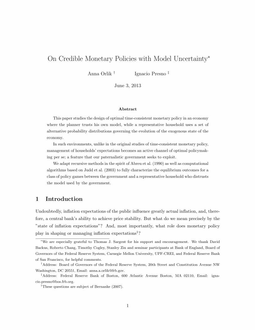
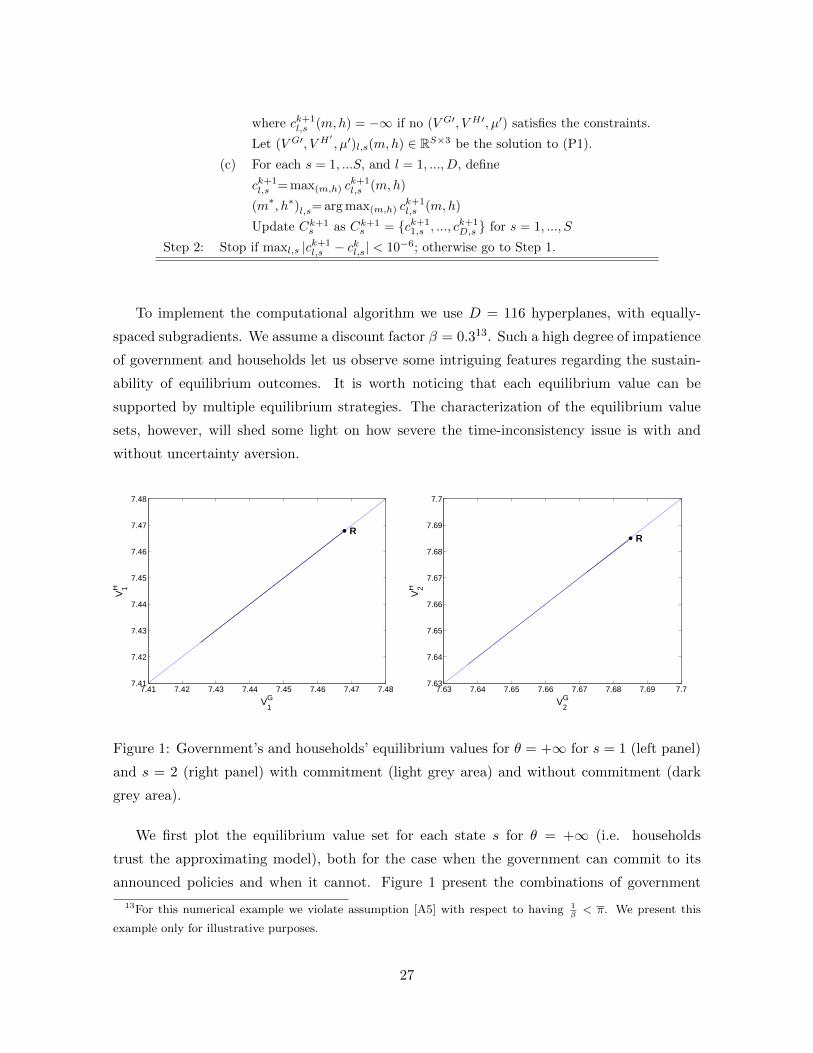
Figure 1: Government’s and households’ equilibrium values for θ = +∞ for s = 1 (left panel)
and s = 2 (right panel) with commitment (light grey area) and without commitment (dark
grey area).
We first plot the equilibrium value set for each state s for θ = +∞ (i.e. households
trust the approximating model), both for the case when the government can commit to its
announced policies and when it cannot. Figure 1 present the combinations of government
13For this numerical example we violate assumption [A5] with respect to having 1β< π. We present this
example only for illustrative purposes.
27
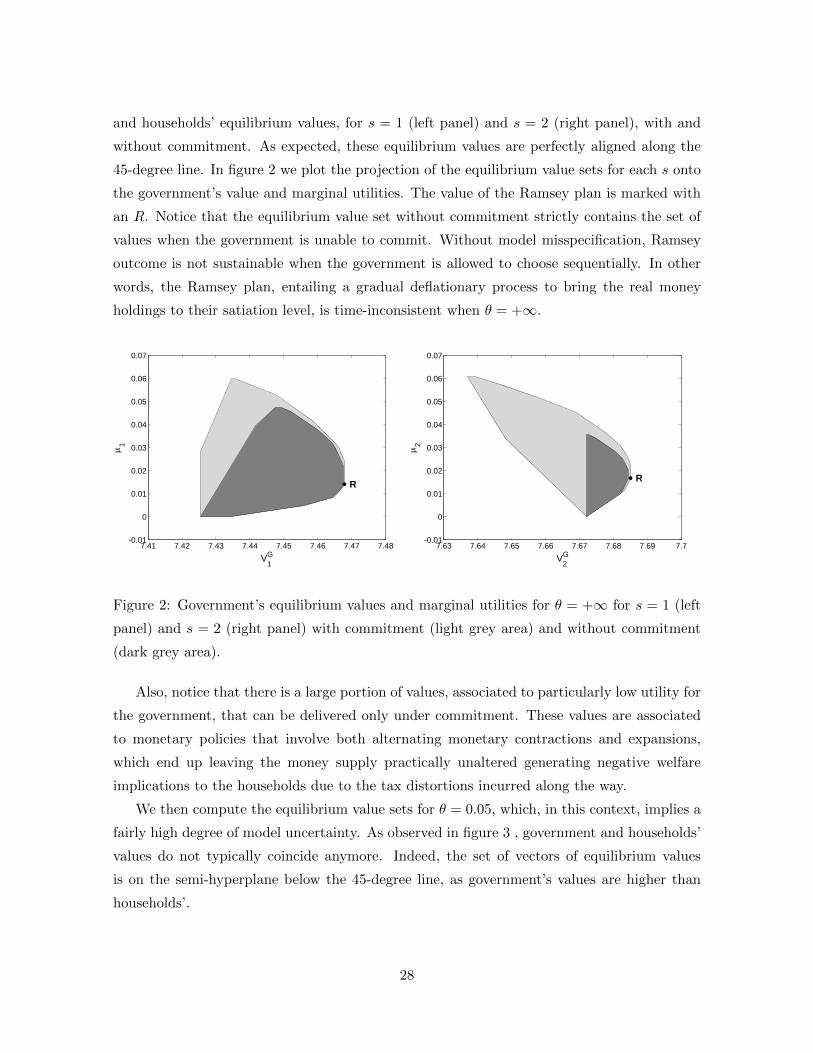
and households’ equilibrium values, for s = 1 (left panel) and s = 2 (right panel), with and
without commitment. As expected, these equilibrium values are perfectly aligned along the
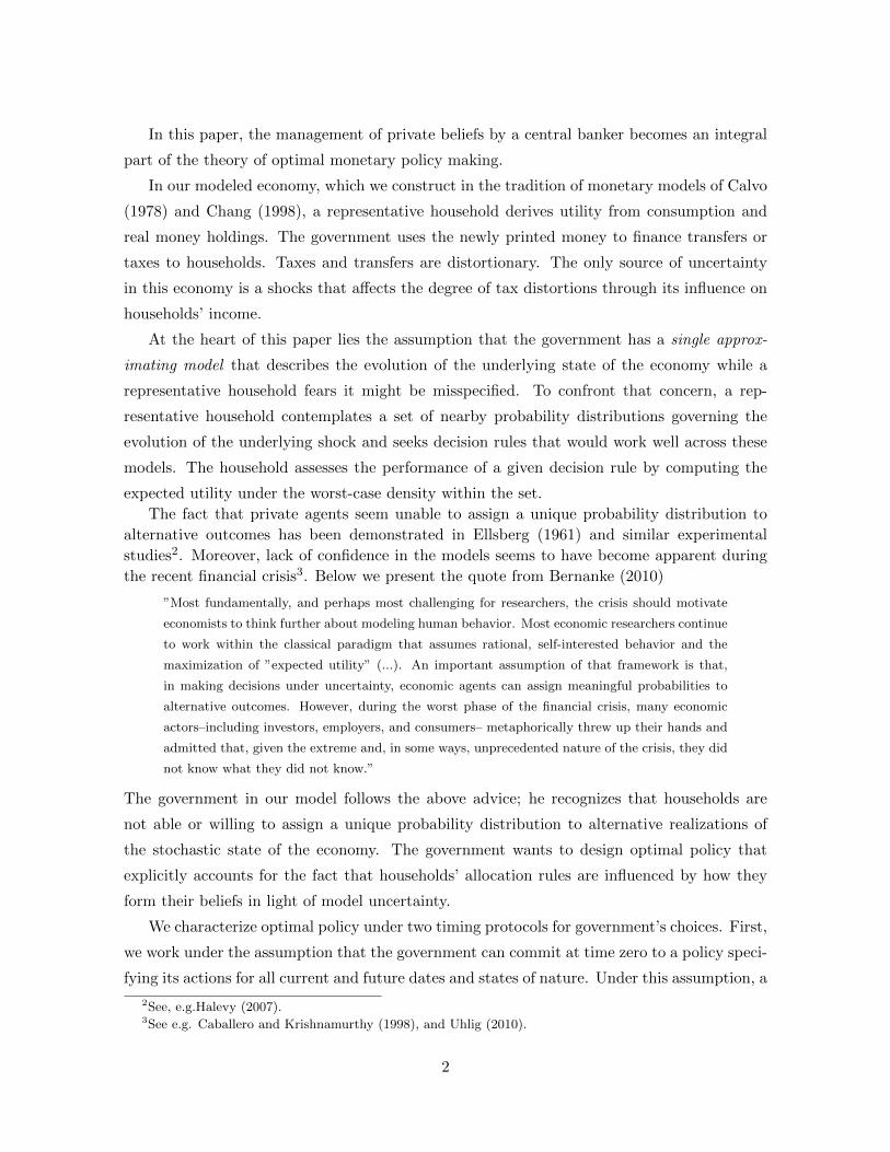
45-degree line. In figure 2 we plot the projection of the equilibrium value sets for each s onto
the government’s value and marginal utilities. The value of the Ramsey plan is marked with
an R. Notice that the equilibrium value set without commitment strictly contains the set of
values when the government is unable to commit. Without model misspecification, Ramsey
outcome is not sustainable when the government is allowed to choose sequentially. In other
words, the Ramsey plan, entailing a gradual deflationary process to bring the real money
holdings to their satiation level, is time-inconsistent when θ = +∞.
7.41 7.42 7.43 7.44 7.45 7.46 7.47 7.48-0.01
0
0.01
0.02
0.03
0.04
0.05
0.06
0.07
VG1
1
R
7.63 7.64 7.65 7.66 7.67 7.68 7.69 7.7-0.01
0
0.01
0.02
0.03
0.04
0.05
0.06
0.07
VG2
2
R
Figure 2: Government’s equilibrium values and marginal utilities for θ = +∞ for s = 1 (left
panel) and s = 2 (right panel) with commitment (light grey area) and without commitment
(dark grey area).
Also, notice that there is a large portion of values, associated to particularly low utility for
the government, that can be delivered only under commitment. These values are associated
to monetary policies that involve both alternating monetary contractions and expansions,
which end up leaving the money supply practically unaltered generating negative welfare
implications to the households due to the tax distortions incurred along the way.
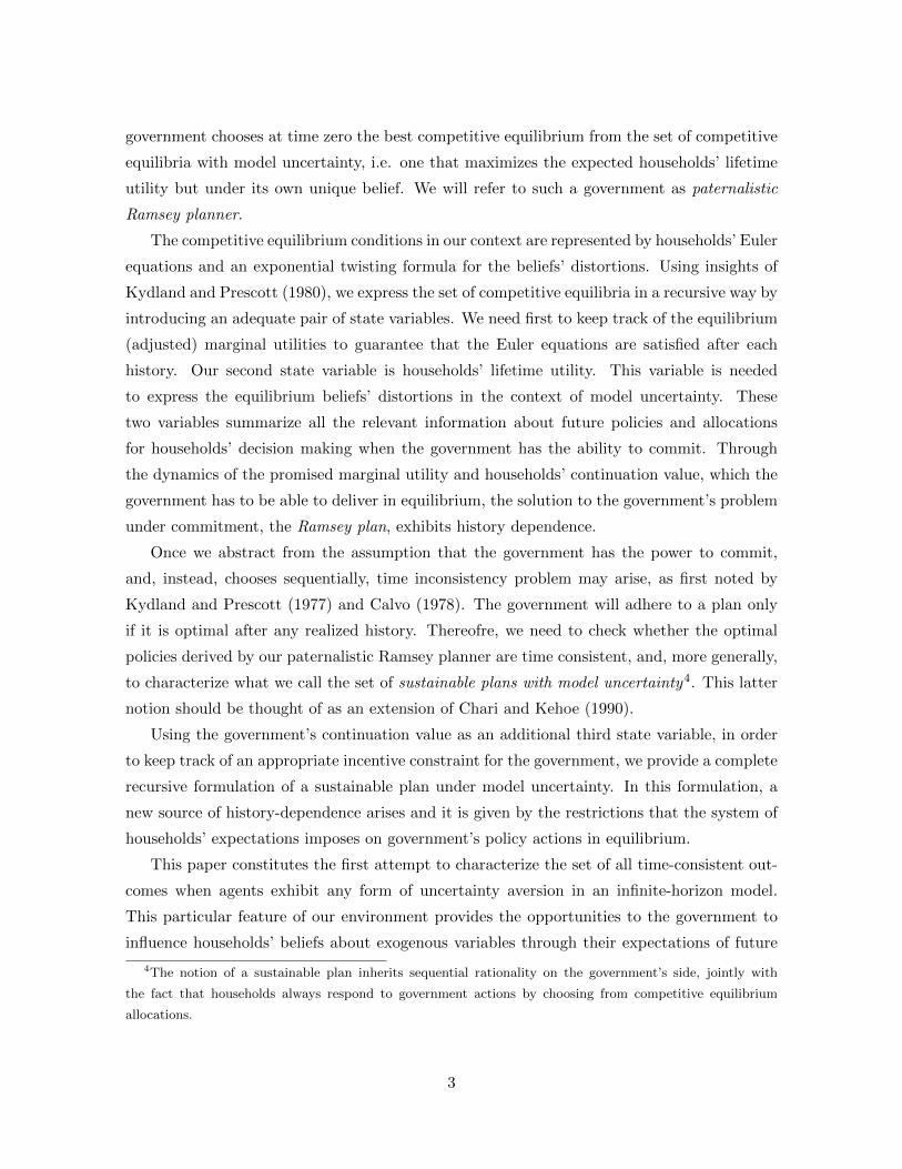
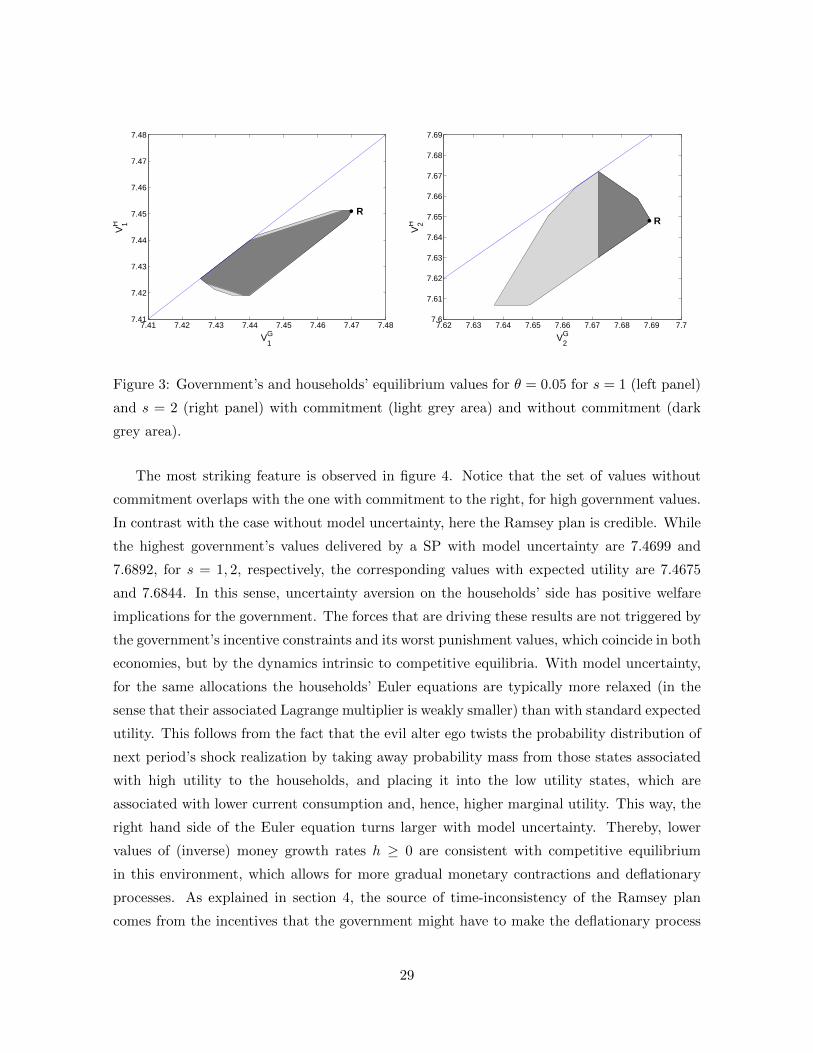
We then compute the equilibrium value sets for θ = 0.05, which, in this context, implies a
fairly high degree of model uncertainty. As observed in figure 3 , government and households’
values do not typically coincide anymore. Indeed, the set of vectors of equilibrium values
is on the semi-hyperplane below the 45-degree line, as government’s values are higher than
households’.
28
7.41 7.42 7.43 7.44 7.45 7.46 7.47 7.487.41
7.42
7.43
7.44
7.45
7.46
7.47
7.48
VG1
VH 1
R
7.62 7.63 7.64 7.65 7.66 7.67 7.68 7.69 7.77.6
7.61
7.62
7.63
7.64
7.65
7.66
7.67
7.68
7.69
VG2
VH 2 R
Figure 3: Government’s and households’ equilibrium values for θ = 0.05 for s = 1 (left panel)
and s = 2 (right panel) with commitment (light grey area) and without commitment (dark
grey area).
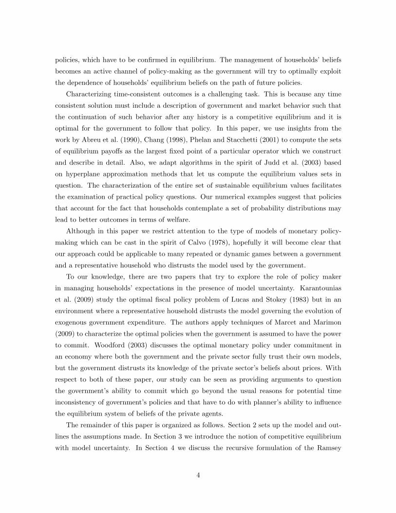
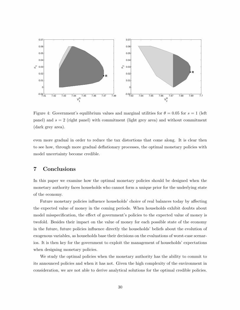
The most striking feature is observed in figure 4. Notice that the set of values without
commitment overlaps with the one with commitment to the right, for high government values.
In contrast with the case without model uncertainty, here the Ramsey plan is credible. While
the highest government’s values delivered by a SP with model uncertainty are 7.4699 and
7.6892, for s = 1, 2, respectively, the corresponding values with expected utility are 7.4675
and 7.6844. In this sense, uncertainty aversion on the households’ side has positive welfare
implications for the government. The forces that are driving these results are not triggered by
the government’s incentive constraints and its worst punishment values, which coincide in both
economies, but by the dynamics intrinsic to competitive equilibria. With model uncertainty,
for the same allocations the households’ Euler equations are typically more relaxed (in the
sense that their associated Lagrange multiplier is weakly smaller) than with standard expected
utility. This follows from the fact that the evil alter ego twists the probability distribution of
next period’s shock realization by taking away probability mass from those states associated
with high utility to the households, and placing it into the low utility states, which are
associated with lower current consumption and, hence, higher marginal utility. This way, the
right hand side of the Euler equation turns larger with model uncertainty. Thereby, lower
values of (inverse) money growth rates h ≥ 0 are consistent with competitive equilibrium
in this environment, which allows for more gradual monetary contractions and deflationary
processes. As explained in section 4, the source of time-inconsistency of the Ramsey plan
comes from the incentives that the government might have to make the deflationary process
29
7.41 7.42 7.43 7.44 7.45 7.46 7.47 7.48-0.01
0
0.01
0.02
0.03
0.04
0.05
0.06
0.07
VG1
1
R
7.63 7.64 7.65 7.66 7.67 7.68 7.69 7.7-0.01
0
0.01
0.02
0.03
0.04
0.05
0.06
0.07
VG2
2
R
Figure 4: Government’s equilibrium values and marginal utilities for θ = 0.05 for s = 1 (left
panel) and s = 2 (right panel) with commitment (light grey area) and without commitment
(dark grey area).
even more gradual in order to reduce the tax distortions that come along. It is clear then
to see how, through more gradual deflationary processes, the optimal monetary policies with
model uncertainty become credible.
7 Conclusions
In this paper we examine how the optimal monetary policies should be designed when the
monetary authority faces households who cannot form a unique prior for the underlying state
of the economy.
Future monetary policies influence households’ choice of real balances today by affecting
the expected value of money in the coming periods. When households exhibit doubts about
model misspecification, the effect of government’s policies to the expected value of money is
twofold. Besides their impact on the value of money for each possible state of the economy
in the future, future policies influence directly the households’ beliefs about the evolution of
exogenous variables, as households base their decisions on the evaluations of worst-case scenar-
ios. It is then key for the government to exploit the management of households’ expectations
when designing monetary policies.
We study the optimal policies when the monetary authority has the ability to commit to
its announced policies and when it has not. Given the high complexity of the environment in
consideration, we are not able to derive analytical solutions for the optimal credible policies.
30

We provide, however, a full characterization the sets of all equilibrium outcomes both with
and without commitment on the government’s side. To compute these sets, we implement a
computational algorithm based on outer hyperplane approximation techniques proposed by
Judd et al. (2003).
The characterization of the set of all sustainable payoffs may shed some light on how severe
the time-inconsistency issue is for the Ramsey plan. As illustrated in our numerical example,
the fact that households may have doubts about model misspecification can help mitigate the
time-inconsistency of the Ramsey plan.
31
A Appendix
A.1 Characterization of the competitive equilibrium sequence
A.1.1 Solving a representative households’ maximization problem
Given pricesqt(s
t)
, government’s policiesht(s
t), xt(st)
and beliefs’ distortionsDt+1
(st+1
), dt+1
(st+1
)∞t=0
, the households’ optimization problem consists of choosingct(st),Mt
(st)∞
t=0and
λt(st), µt(st)∞
t=0to maximize and minimize, respectively, the
lagrangian
LH =∞∑t=0
βt∑st
π(st)Dt(st)[u(ct(st))
+ v(qt(st)Mt
(st))]
+
−λt(st) [qt(st)Mt
(st)− yt
(st)
+ xt(st)
+ ct(st)− qt
(st)Mt−1
(st−1
)]+
− µt(st) [qt(st)Mt
(st)−m
]Taking FOCs we obtain
u′(ct(st)) = λt
(st)
(24)
Dt(st)[v′(mt
(st))qt(st)− λt
(st)qt(st)]
+
β∑st+1
π(st+1|st)λt+1
(st+1
)Dt+1(st+1)qt+1
(st+1
)−Dt(s
t)µt(st)qt(st)
= 0 (25)
Substitute equation (24) into (25), use (2) and note thatqt+1(st+1)qt(st)
=mt+1(st+1)ht+1(st+1)
mt(st)
v′(mt
(st))− u′(ct
(st)) + β
∑st+1
π(st+1|st)Dt+1(st+1)
Dt(st)u′(ct+1
(st+1
))qt+1
(st+1
)qt (st)
≥ 0,
= 0 if mt
(st)< m
mt
(st) [u′(ct
(st))− v′(mt
(st))]
−β∑st+1
π(st+1|st)dt+1
(st+1|st
)u′(ct+1
(st+1
))mt+1
(st+1
)ht+1
(st+1
)≤ 0,
= 0 if mt
(st)< m
The above expression is our equilibrium condition, equation (10).
A.1.2 Solving alter ego’s minimization problem
Given ct(st),mt(s
t), the evil alter ego’s optimization problem consists of choosingDt
(st), dt+1(st+1|st)
and
φt+1
(st+1
), ϕt
(st)
to minimize and maximize, respectively,
32
the lagrangian
LAE =
∞∑t=0
βt∑st
πt(st)Dt(s
t)[u(ct) + v(mt)] +
+βθ∑st+1
π(st+1|st)dt+1(st+1|st) log dt+1(st+1|st)+
−β∑st+1
π(st+1|st)φt+1
(st+1
) [Dt+1(st+1)− dt+1(st+1|st)Dt(s
t)]
+
−ϕt(st)∑
st+1
π(st+1|st)dt+1(st+1|st)− 1
The FOCs for dt+1(st+1|st) and Dt(s
t) are respectively given by
βθDt(st) [log dt+1(st+1|st) + 1] + βφt+1
(st+1
)Dt(s
t) = ϕt(st)
(26)
[u(ct) + v(mt)] + βθ∑st+1
π(st+1|st)dt+1(st+1|st) log dt+1(st+1|st)+
+β∑st+1
π(st+1|st)φt+1
(st+1
)dt+1(st+1|st) = φt
(st)
(27)
Rearranging (26) leads to
log dt+1(st+1|st) = −1 +ϕt(st)
βθDt(st)−φt+1
(st+1
)θ
dt+1(st+1|st) = exp
(−1 +
ϕt(st)
βθDt(st)
)exp
(−φt+1
(st+1
)θ
)(28)
By condition (3) it has to be the case that
exp
(−1 +
ϕt(st)
βθDt(st)
)∑st+1
π(st+1|st) exp
(−φt+1
(st+1
)θ
)= 1
exp
(−1 +
ϕt(st)
βθDt(st)
)=
1∑st+1
π(st+1|st) exp(−φt+1(st+1)
θ
) (29)
Substituting equation (29) back into (28) yields
dt+1(st+1|st) =
exp
(−φt+1(st+1)
θ
)∑
st+1π(st+1|st) exp
(−φt+1(st+1)
θ
) (30)
Now we use (26) and impose a respective transversality condition,
limt→∞
βt∑st+1
π(st+1|st)φt+1
(st+1
)dt+1(st+1|st) = 0 (31)
33
It follows that
φt(st)
= V Ht
(st)
(32)
Using the above result in equation (30) delivers our equilibrium condition (11)
dt+1(st+1|st) =
exp
(−V Ht+1(st+1)
θ
)∑
st+1π(st+1|st) exp
(−V Ht+1(st+1)
θ
)A.1.3 On transversality condition
We will show that the transversality condition,
βt∑
st+1π(st+1|st)dt+1(st+1|st)u′
[(f(xt
(st), st)
]mt
(st)ht(st)→ 0 as t → ∞ for all t and
all st, is satisfied if (m,x,h,d,VH) ∈ E∞.
Since E is compact, for any(xt(st),mt
(st), ht(st), dt+1(st+1|st)
)∈ E, it must be that∑
st+1π(st+1|st)dt+1(st+1|st)u′
[(f(xt
(st), st)
]mt
(st)ht(st)
belongs to a compact interval
(due to continuity of u′ and f) for every t. Hence, it has to be that∑st+1
π(st+1|st)dt+1(st+1|st)u′[(f(xt
(st), st)
]mt
(st)ht(st)
is a bounded sequence, and the
required sequence indeed converges to zero.
A.2 Example of competitive equilibrium sequences
Assume that st = H,L and that the production function is such that f(0, H) = f(0, L). Set
(m,x,h) = m∗, 0, 1∞t=0 where m∗ satisfies the following condition for all t and all st
u′ (f(0, st)) (1− β) = v′ (m∗)
Then (m,x,h) ∈ CEs.
A.3 Proof of Corollary 3.
CEs for all s ∈ S is compact.
Proof. Fix s0 ∈ S. Let(mn,xn,hn,dn,VHn)
be the sequence from CEs=s0 converging to
some sequence(m,x,h,d,VH
). We need to show that this limiting sequence belongs to
CEs=s0 .
CEs=s0 is a nonempty subset of a compact set E∞. Since E∞ is compact, it is closed, and,
hence,(m,x,h,d,VH
)∈ E∞.
The fact that(mn,xn,hn,dn,VHn) ∈ CEs=s0 implies that equations (10) - (13) are
satisfied for each n. Consequently, by continuity of u, v, u′, v′ and f ,(m,x,h,d,VH
)satisfy
34

these same equations. It follows then from Proposition 3.1 that(m,x,h,d,VH
)∈ CEs=s0 ,
which means that CEs=s0 is a closed subset of the compact set. Hence, it is compact.
35
References
Abreu, D., D. Pearce, and E. Stacchetti (1990). Toward a theory of discounted repeated
games with imperfect monitoring. Econometrica 58 (5), 1041–1063.
Abreu, D. and Y. Sannikov. An algorithm for two player repeated games with perfect moni-
toring. Economic Theory Center Working Paper No. 26-2011 .
Bernanke, B. S. (2007). Inflation expectations and inflation forecasting. Speech at the Mone-
tary Economics Workshop of the National Bureau of Economic Research Summer Institute,
Cambridge, Massachusetts.
Bernanke, B. S. (2010). Implications of the financial crisis for economics. Speech at the
Conference Co-sponsored by the Center for Economic Policy Studies and the Bendheim
Center for Finance, Princeton University, Princeton, New Jersey .
Caballero, R. J. and A. Krishnamurthy (1998). Collective risk management in a flight to
quality episode. Journal of Finance (5), 2195–2230.
Calvo, G. A. (1978). On the time consistency of optimal policy in a monetary economy.
Econometrica 46 (6), 1411–1428.
Chang, R. (1998). Credible monetary policy in an infinite horizon model: Recursive ap-
proaches. Journal of Economic Theory 81 (6), 431–461.
Chari, V. V. and P. Kehoe (1990). Sustainable plans. Journal of Political Economy 98 (4),
783–802.
Ellsberg, D. (1961). Risk, ambiguity and savage axioms. Quarterly Journal of Eco-
nomics 75 (4), 643–669.
Fernandez-Villaverde, J. and A. Tsyvinski (2002). Optimal fiscal policy in a business cycle
model without commitment. Mimeo, University of Pennsylvania.
Halevy, Y. (2007). Ellsberg revisited: An experimental study. Econometrica 75 (2), 503–536.
Hansen, L. P. and T. J. Sargent (2007). Recursive robust estimation and control without
commitment. Journal of Economic Theory 136 (1), 1–27.
Hansen, L. P. and T. J. Sargent (2008). Robustness. Princeton, NJ; Princeton University
Press.
36
Judd, K., S. Yeltekin, and J. Conklin (2003). Computing supergame equilibria. Economet-
rica 71 (4), 1239–1254.
Karantounias, A. G., L. P. Hansen, and T. J. Sargent (2009). Managing expectations and
fiscal policy. Federal Reserve Bank of Atlanta Working Paper 2009-29 .
Kydland, F. and E. C. Prescott (1977). Rules rather than discretion: The inconsistency of
optimal plans. Journal of Political Economy 85 (3), 473–491.
Kydland, F. and E. C. Prescott (1980). Dynamic optimal taxation, rational expectations and
optimal control. Journal of Economic Dynamics and Control 2, 79–91.
Ljungqvist, L. P. and T. J. Sargent (2004). Recursive Macroeconomic Theory. The MIT Press;
Cambridge, MA.
Lucas, R. E. and N. L. Stokey (1983). Optimal fiscal and monetary policy in an economy
without capital. Journal of Monetary Economics 12 (1), 55–93.
Marcet, A. and R. Marimon (2009). Recursive contracts. Mimeo, Institut d’ Analisi
Economica.
Phelan, C. and E. Stacchetti (2001). Sequential equilibria in a ramsey tax model. Economet-
rica 69 (6), 1491–1518.
Uhlig, H. (2010). A model of a systemic bank run. Journal of Monetary Economics 57 (1),
78–96.
Woodford, M. (2003). Interest and prices: Foundations of a theory of monetary policy.
Princeton University Press.
37