Tellus (2008), 60A, 620–631 C© 2008 The AuthorsJournal compilation C© 2008 Blackwell Munksgaard

Printed in Singapore. All rights reservedT E L L U S

Climate mode simulation of North Atlantic polar lowsin a limited area model

By MATTHIAS ZAHN 1,2∗, HANS VON STORCH 1,2 and STEPHAN BAKAN 3, 1Institute for CoastalResearch GKSS Research Center, System Analysis and Modelling, Max-Planck-Straße 1, D-21502 Geesthacht,

Germany; 2Meteorological Institute of the University of Hamburg, Bundesstr. 55, D-20146 Hamburg, Germany;3Max Planck Institute for Meteorology, Bundesstr. 53, D-20146 Hamburg, Germany

(Manuscript received 18 June 2007; in final form 10 March 2008)

ABSTRACTPolar lows are not properly resolved in global re-analyses. In order to describe the year-to-year variability and decadaltrends in the formation of such mesoscale storms, atmospheric limited area models, which post-process re-analysis data,may be an appropriate tool. In this study we demonstrate the merits and potential of this approach.

A series of 3-week long ensemble simulations of weather situations over the NE Atlantic with a limited areamodel/regional climate model (CLM) are examined. The model was driven with NCEP–NCAR re-analyses at thelateral and lower boundaries. Additionally, the spectral nudging technique was used to enforce the large-scale circula-tion, as given by the NCEP–NCAR reanalysis, on the simulation. The ensemble members differ by initial conditionstaken from several consecutive days.

In most of the cases, a polar low developed after a simulated time of about 2 weeks, that is, long after the initializationof the model calculations.

The spectrally nudged version of the model is very insensitive to initial conditions. The observed polar lows werereproduced in all ensemble members. A reasonable correlation between the simulated polar low features and thosederived from a satellite product (HOAPS-III) and operational high-resolution weather analyses (DWD) is found. Thepolar lows are considerably deepened compared to the driving NCEP–NCAR analysis, but the comparison with weathermaps indicates some differences in detail.

When CLM is run without the large-scale constraint of spectral nudging, considerable variability emerges across thedifferent ensemble members and the observed polar low often does not emerge.

1. Introduction

The term polar low is used for a spectrum of different intensemaritime small and mesoscale (horizontal diameter up to 1000km) cyclones forming poleward the Polar Front in both hemi-spheres (Rasmussen and Turner, 2003). Because they are asso-ciated with surface wind speeds near or above gale force, severeweather and heavy precipitation, they constitute a significant partof the marine weather risk in subpolar waters.

A variety of initial conditions and forcing mechanisms, whichusually interact with each other, are thought of as being re-sponsible for polar low development. Early studies focused onbaroclinic environments as an initial condition for polar lowdevelopment (e.g. Harrold and Browning, 1969) as well asapproaching upper level disturbances (Harrold and Browning,

∗Corresponding author.e-mail: matthias.zahn@gkss.deDOI: 10.1111/j.1600-0870.2008.00330.x

1969; Rasmussen, 1985). To explain their further developmentconditional instability of the second kind (e.g. Rasmussen, 1979)and air sea interaction instability (Emanuel, 1986; Emanuel andRotunno, 1989), subsequently renamed Wind Induced SurfaceHeat Exchange, are considered as being important for polar lowdevelopment.

More recently a wealth of sensitivity and diagnostic studiesof polar low occurrences in the North Atlantic applying highresolution numerical models were undertaken to increase theunderstanding of the dynamical processes involved (Nordengand Rasmussen, 1991; Grønas and Kvamstø, 1995; Mailhotet al., 1996; Nielsen, 1997; Claud et al., 2004). Further nu-merical studies were undertaken for other parts in the NorthernHemisphere by Yanase et al. (2002, 2004) for the Japan Sea,Blier (1996) and Bresch et al. (1997) for the Gulf of Alaska andLee et al. (1998) for the Korean Peninsula as well as for theAntarctic (Heinemann, 1998; Heinemann and Klein, 2003). Allof them succeed in reproducing the respective polar low casereasonably.

620 Tellus 60A (2008), 4

P U B L I S H E D B Y T H E I N T E R N A T I O N A L M E T E O R O L O G I C A L I N S T I T U T E I N S T O C K H O L M

SERIES ADYNAMIC METEOROLOGYAND OCEANOGRAPHY

CLIMATE MODE SIMULATION OF POLAR LOWS 621

In addition to these process studies, studies focusing onclimatological aspects of mesocyclones and polar lows wereconducted in the northern (Wilhelmsen, 1985; Harold et al.,1999a,b) as well as in the southern hemisphere (e.g. Carleton andCarpenter, 1990). As these studies were primarily based on satel-lite imagery or observations, they only describe a limited timeperiod and also suffer from a lack of homogeneity. Further un-certainties emerge from the subjective way of detection. A firstobjective climatology of polar lows was compiled by Bracegir-dle and Gray (2008) based on applying objective criteria forthe identification of polar lows to numerical weather predictiondata. However these data were available for a relatively shorttime period only.

The construction of comprehensive multidecadal climatolog-ical statistics of polar low occurrences has not been achievedso far. However, such knowledge is needed to assess interan-nual variability and decadal trends, and for evaluating possibleconnections or contributions to larger scale climatic changes inthe past and future. Presently available long-term databases, thatpossibly enable an assessment of such questions, usually sufferfrom inhomogeneities, that is, changes over time are related tochanging analysis tools and skills. However, data homogeneityis a key requisite for robust assessments of ongoing change.

We have begun to implement a technique which we hope willallow us to overcome the limitation of too short and inhomoge-neous data. The basic idea is to run an atmospheric limited areamodel covering the NE Atlantic with global re-analyses at the lat-eral and lower boundaries. Additionally a large-scale constraintapplied in the interior to impose the reliably and homogeneouslyanalysed large-scale atmospheric state on the mesoscale forma-tion and life cycle of polar lows. Recently, such re-analysis datawas used by Kolstad (2006) to detect ‘reverse shear flow’ atmo-spheric conditions, which favour the development of a particularkind of polar low. Also using the relatively coarsely gridded re-analysis data, Condron et al. (2006) investigated climatologicalaspects of mesocyclones by locating the maxima in the Laplacianof the pressure field or geopotential height.

In this paper, we want to investigate whether a higher reso-lution atmospheric limited area model (LAM)/regional climatemodel (RCM), as used in long term retrospective reconstructionsof the detailed weather stream (e.g. Weisse et al., 2005), is capa-ble of reproducing such subpolar maritime mesoscale features. Indoing so, we implicitly assume the validity of the ‘downscalingconcept’, namely that the interaction of a given large-scale flowwith the regional physiographic details will cause the formationof mesoscale features.

The above mentioned sensitivity or diagnostic studies are con-ducted in order to accurately simulate the dynamical processesinvolved in polar low development. Therefore, the best possiblelarge-scale fields are used as initial fields, which usually are closeto the times of the respective polar low occurrences. Contrary tothose studies we want to investigate if and how well polar lowscan be reproduced in climate mode simulations, which are ini-

tialized long before their formation. The formation takes placeapproximately 2 weeks after initialization and thus is not directlydependent on the initial state, but depends on the constraintsplaced on the model at its boundaries and on its large-scale state.

In this study we present results from a feasibility study, as towhether our dynamical downscaling set-up of an atmosphericlimited area model run in climate mode is indeed generating theadditional mesoscale information. Therefore, on the one handwe drive the model in the conventional way forced at the mar-gins and on the second hand we additionally make use of thespectral nuding technique (von Storch et al., 2000) to enforce agiven large-scale onto the simulations. We examine in a series ofthree independent case studies, if and how good polar lows arereproduced in such a set-up. Therefore, 3-week long ensemble-simulations with a LAM/RCM were undertaken for three polarlow occurrences and compared to observational data.

In Section 2, we describe the used LAM/RCM, its setup andthe observational data, in Section 3 we describe the general re-sults for the first case in Section 3.1 and for the mesoscale inSection 3.2. In Section 3.3, the results for the two other cases areshown. We end with a summary and conclusion in Section 4.

2. Regional model and simulations

The LAM/RCM applied in the present study is the atmosphericlimited area model CLM (http://clm-community.eu) (Bohmet al., 2006). CLM is the climate version of the ‘Lokal Model’LM (Steppeler et al., 2003) of the German Weather Service. Itsprognostic, non-hydrostatic equations feature the variables hor-izontal and vertical wind, real temperature, pressure, specifichumidity and specific cloud liquid water content on a hybridcoordinate system with 32 σ -levels. Initial and lateral boundaryvalues are provided by the NCEP–NCAR re-analyses (Kalnay etal., 1996). The latter are available every 6 h with a grid resolutionof 2◦ (∼220 km) and are nudged in a lateral ‘sponge zone’ to-wards the NCEP–NCAR re-analyses (Davies, 1976). CLM hasbeen used for a number of climatological investigations (e.g.Bohm et al., 2004; Deque et al., 2005; Woth et al., 2006) but sofar not for investigations in polar regions.

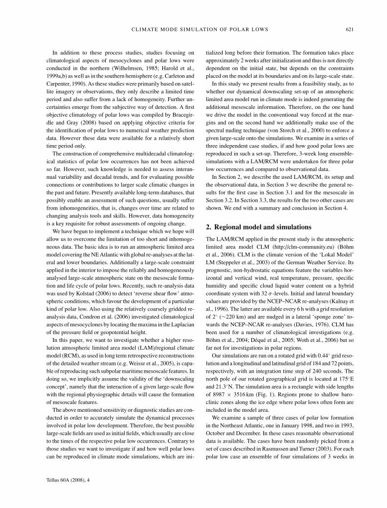
Our simulations are run on a rotated grid with 0.44◦ grid reso-lution and a longitudinal and latitudinal grid of 184 and 72 points,respectively, with an integration time step of 240 seconds. Thenorth pole of our rotated geographical grid is located at 175◦Eand 21.3◦N. The simulation area is a rectangle with side lengthsof 8987 × 3516 km (Fig. 1). Regions prone to shallow baro-clinic zones along the ice edge where polar lows often form areincluded in the model area.

We examine a sample of three cases of polar low formationin the Northeast Atlantic, one in January 1998, and two in 1993,October and December. In these cases reasonable observationaldata is available. The cases have been randomly picked from aset of cases described in Rasmussen and Turner (2003). For eachpolar low case an ensemble of four simulations of 3 weeks in

Tellus 60A (2008), 4

622 M. ZAHN ET AL.

280˚

290˚

300˚

310˚

320˚

330˚

340˚

350˚ 0˚

10˚

20˚

30˚

40˚

50˚

60˚

70˚

80˚

90˚280˚

290˚

300˚

310˚

320˚

330˚

340˚

350˚ 0˚

10˚

20˚

30˚

40˚

50˚

60˚

70˚

80˚

90˚

Fig. 1. Model grid used for this study.Darker grid boxes at the border represent thesponge zone.

length was performed. All simulations are begun about 2 weeksprior to the formation of the polar low, so that the dynamicaldevelopment should be independent of the details of the initial-ization. The members of the respective ensembles differ by theirinitial date. They are separated by 24 h in order to create different,but consistent, initial states.

One ensemble was performed with constraining CLM only atthe lateral boundaries and by the SST and sea ice conditions;these simulations are named ‘non-nudged’ (CLM-nn). A secondset of ensembles additionally makes use of spectral nudging (vonStorch et al., 2000), referred to as CLM-sn. Spectral nudgingis a mathematical method used to enforce a given large-scalefield in the simulation of the LAM. Experiments (Feser, 2006)have demonstrated that, while the large-scale circulations areefficiently constrained, the mesoscale variability conditioned bythe given large-scale state is not significantly limited by thisprocedure. The key parameter for spectral nudging is the spectralrange, within which the constraint is acting. Here we have chosenzonal wave numbers up to 14 relative to 8987 km and meridionalwave numbers up to 5 relative to 3516 km as being constraint(corresponding to a spatial scale of approximately 700 km andmore). The constraint is implemented with a vertically growingstrength (α = 0.5; von Storch et al., 2000) at 850 hPa and above.

To assess the realism of the simulation data we compared itwith a number of observation based data sources. First, the man-ually drawn mean sea level pressure maps from Berliner Wet-terkarte and from the German Meteorological Service (DWD)are applied. Also originating from the DWD a second data setcomprises the operational regional analyses available from 1993until 1998 with a grid resolution of 0.5◦.

A third data set contains almost instantaneous wind speedsfrom satellite soundings in the Hamburg Ocean AtmosphereParameters and Fluxes from Satellite Data set (HOAPS,Andersson et al. (2007); www.hoaps.org). For the present studythe HOAPS data were available between 1988 and 2002 ona regular grid of 0.5◦ for individual satellite overpasses. Theapplied wind algorithm uses a neural network to infer windspeed at 10 m height above the sea surface from Special SensorMicrowave/Imager (SSM/I) measurements. It consists of aninput layer for the brightness temperatures of 5 microwavechannels, a hidden layer with three neurons and an output layer

containing the wind speed. The network was trained with a com-posite data set from buoy measurements and radiative transfersimulations. The accuracy of these wind speed data is estimatedat about 1.5 m s−1 from theoretical considerations and obser-vational comparison studies. In contrast to the first two dataproducts, the HOAPS wind fields are not available at synopticdates but instantaneously during satellite overpasses and they aregenerally only partially filled along satellite swaths.

3. Results

In this section, first the model’s general ability to describe onepolar low case including its track is presented and the large-scalecirculation in the analyses and model simulations are compared.Secondly, details of this polar low formation are considered.This is done by filtering out large-scale components, so thatonly mesoscale features enter the analysis. Finally, results fortwo other cases are discussed.

3.1. Comparison of simulations with analysesand observations

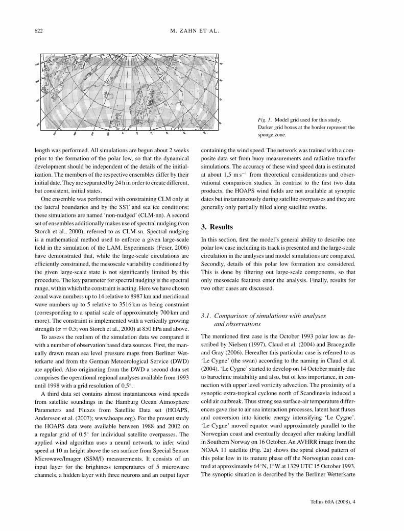
The mentioned first case is the October 1993 polar low as de-scribed by Nielsen (1997), Claud et al. (2004) and Bracegirdleand Gray (2006). Hereafter this particular case is referred to as‘Le Cygne’ (the swan) according to the naming in Claud et al.(2004). ‘Le Cygne’ started to develop on 14 October mainly dueto baroclinic instability and also, but of less importance, in con-nection with upper level vorticity advection. The proximity of asynoptic extra-tropical cyclone north of Scandinavia induced acold air outbreak. Thus strong sea surface-air temperature differ-ences gave rise to air sea interaction processes, latent heat fluxesand conversion into kinetic energy intensifying ‘Le Cygne’.‘Le Cygne’ moved equator ward approximately parallel to theNorwegian coast and eventually decayed after making landfallin Southern Norway on 16 October. An AVHRR image from theNOAA 11 satellite (Fig. 2a) shows the spiral cloud pattern ofthis polar low in its mature phase off the Norwegian coast cen-tred at approximately 64◦N, 1◦W at 1329 UTC 15 October 1993.The synoptic situation is described by the Berliner Wetterkarte

Tellus 60A (2008), 4

CLIMATE MODE SIMULATION OF POLAR LOWS 623

Fig. 2. (a) AVHRR NOAA 11 satellite image at 1329 UTC 15 July 1993 (adapted from Claud et al., 2004), and (b) surface weather chart from theFree University of Berlin at 0700 UTC 15 October 1993 (Berliner Wetterkarte 1993).

in Fig. 2b, with a synoptic low pressure system at the northerntip of Scandinavia and the small polar low at about 65◦N, 2◦E.

For this case two ensembles of four nudged and four non-nudged simulations were started at 0000 UTC on 1, 2, 3 and 4October 1993, respectively. These simulations are named refer-ring to the day of initialisation, namely CLM01-sn, CLM02-sn,CLM03-sn and CLM04-sn for the nudged ones and CLM01-nn, CLM02-nn, CLM03-nn and CLM04-nn for the non-nudgedruns.

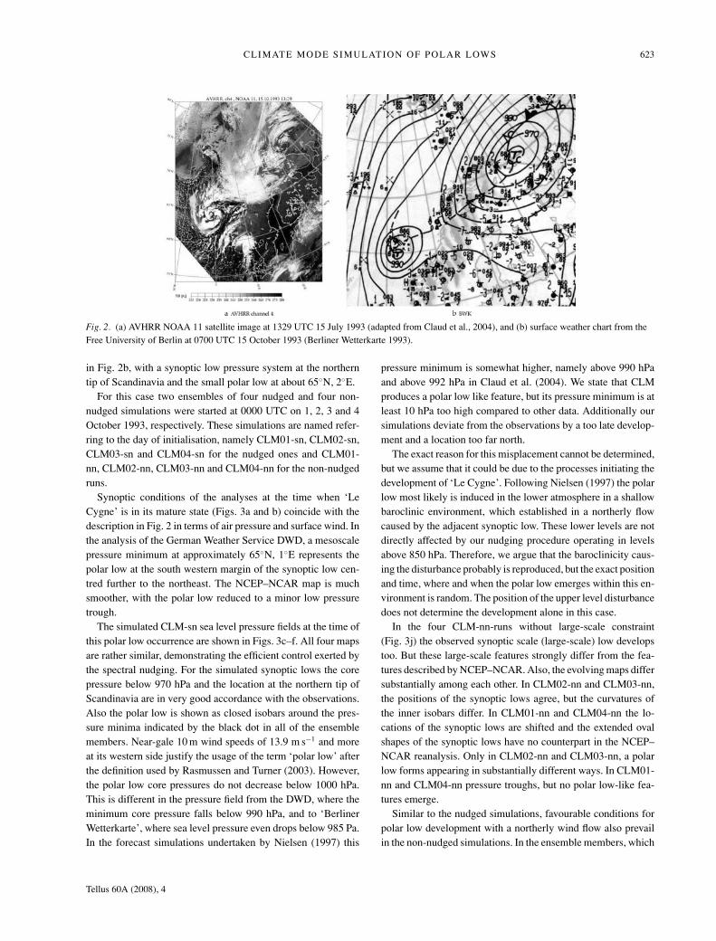
Synoptic conditions of the analyses at the time when ‘LeCygne’ is in its mature state (Figs. 3a and b) coincide with thedescription in Fig. 2 in terms of air pressure and surface wind. Inthe analysis of the German Weather Service DWD, a mesoscalepressure minimum at approximately 65◦N, 1◦E represents thepolar low at the south western margin of the synoptic low cen-tred further to the northeast. The NCEP–NCAR map is muchsmoother, with the polar low reduced to a minor low pressuretrough.

The simulated CLM-sn sea level pressure fields at the time ofthis polar low occurrence are shown in Figs. 3c–f. All four mapsare rather similar, demonstrating the efficient control exerted bythe spectral nudging. For the simulated synoptic lows the corepressure below 970 hPa and the location at the northern tip ofScandinavia are in very good accordance with the observations.Also the polar low is shown as closed isobars around the pres-sure minima indicated by the black dot in all of the ensemblemembers. Near-gale 10 m wind speeds of 13.9 m s−1 and moreat its western side justify the usage of the term ‘polar low’ afterthe definition used by Rasmussen and Turner (2003). However,the polar low core pressures do not decrease below 1000 hPa.This is different in the pressure field from the DWD, where theminimum core pressure falls below 990 hPa, and to ‘BerlinerWetterkarte’, where sea level pressure even drops below 985 Pa.In the forecast simulations undertaken by Nielsen (1997) this

pressure minimum is somewhat higher, namely above 990 hPaand above 992 hPa in Claud et al. (2004). We state that CLMproduces a polar low like feature, but its pressure minimum is atleast 10 hPa too high compared to other data. Additionally oursimulations deviate from the observations by a too late develop-ment and a location too far north.

The exact reason for this misplacement cannot be determined,but we assume that it could be due to the processes initiating thedevelopment of ‘Le Cygne’. Following Nielsen (1997) the polarlow most likely is induced in the lower atmosphere in a shallowbaroclinic environment, which established in a northerly flowcaused by the adjacent synoptic low. These lower levels are notdirectly affected by our nudging procedure operating in levelsabove 850 hPa. Therefore, we argue that the baroclinicity caus-ing the disturbance probably is reproduced, but the exact positionand time, where and when the polar low emerges within this en-vironment is random. The position of the upper level disturbancedoes not determine the development alone in this case.

In the four CLM-nn-runs without large-scale constraint(Fig. 3j) the observed synoptic scale (large-scale) low developstoo. But these large-scale features strongly differ from the fea-tures described by NCEP–NCAR. Also, the evolving maps differsubstantially among each other. In CLM02-nn and CLM03-nn,the positions of the synoptic lows agree, but the curvatures ofthe inner isobars differ. In CLM01-nn and CLM04-nn the lo-cations of the synoptic lows are shifted and the extended ovalshapes of the synoptic lows have no counterpart in the NCEP–NCAR reanalysis. Only in CLM02-nn and CLM03-nn, a polarlow forms appearing in substantially different ways. In CLM01-nn and CLM04-nn pressure troughs, but no polar low-like fea-tures emerge.

Similar to the nudged simulations, favourable conditions forpolar low development with a northerly wind flow also prevailin the non-nudged simulations. In the ensemble members, which

Tellus 60A (2008), 4

624 M. ZAHN ET AL.

Fig. 3. 10 m wind speed ≥13.9 m s−1 and air pressure (at mean sea level) at 0600 UTC 15 October 1993: (a) DWD analysis data, (b) NCEP–NCARanalysis after interpolation onto the CLM grid, 0600 UTC, (c–f) CLM ensemble run with spectral nudging and (g–j) without, 0900 UTC,initialization times of the simulations are 1–4 October, respectively. If existent, black dots indicate the positions of the polar low’s pressure minimumin the respective run.

do not reproduce the polar low, the synoptic low is located fartherwest. Thus the synoptic low’s back circulation, the area in whichthe polar low develops, is shifted farther west into regions lessaffected by the warm water supply of the gulf stream. We sug-gest that lower surface temperatures, and thus a smaller air–seatemperature difference, inhibit the transformation of a mesoscaledevelopment into the polar low.

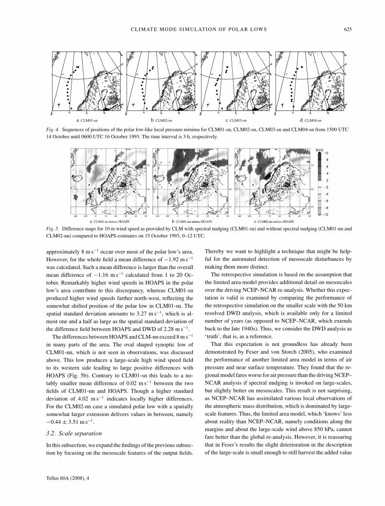
We developed a simple algorithm to track the local surfacepressure minima. Based on manually provided coordinates at1500 UTC 14 October 1993, when the polar low emerged, thisalgorithm finds the nearest local minimum in the next time step(3 h) of the output data and so on. The resulting sequences ofpositions for CLM-sn are illustrated in Fig. 4 and can be inter-preted as tracks of the simulated polar low. In all four cases,these tracks are very similar. Following a north–south direc-tion, they are in accordance with the track described in Nielsen(1997).

In CLM01-nn and CLM04-nn a track could not be identifiedbecause clear pressure minima were lacking. The polar low-likefeatures in CLM02-nn and CLM03-nn developed very close tothe Norwegian coast, remained there and made landfall nearTrondheim leading to wrong tracks (not shown).

We compared the instantaneous satellite-derived wind speedestimates (HOAPS) with the simulated fields; only CLM01-snis considered (Fig. 5a)—the other three sn-cases are virtuallyidentical. For the ‘nn’ ensemble we show two cases, namelyCLM01-nn without the formation of a polar low (Fig. 5b) andCLM02-nn with such a formation (Fig. 5c). We think that theseinstantaneous wind speeds are suitable for representing the windfield pattern.

This comparison also reveals the advantage of the nudged sim-ulations. Differences generated between HOAPS and CLM01-sn show the smoothest pattern. Apart from higher CLM windspeed off the coast of Southern Norway, differences larger than

Tellus 60A (2008), 4

CLIMATE MODE SIMULATION OF POLAR LOWS 625

350˚ 0˚

10˚

20˚

30˚40˚

50˚

60˚

70˚

350˚ 0˚

10˚

20˚

30˚40˚

50˚

60˚

70˚

a CLM01-sn35

0˚ 0˚

10˚

20˚

30˚40˚

50˚

60˚

70˚

350˚ 0˚

10˚

20˚

30˚40˚

50˚

60˚

70˚

b CLM02-sn

350˚ 0˚

10˚

20˚

30˚40˚

50˚

60˚

70˚

350˚ 0˚

10˚

20˚

30˚40˚

50˚

60˚

70˚

c CLM03-sn

350˚ 0˚

10˚

20˚

30˚40˚

50˚

60˚

70˚

350˚ 0˚

10˚

20˚

30˚40˚

50˚

60˚

70˚

d CLM04-sn

Fig. 4. Sequences of positions of the polar low-like local pressure minima for CLM01-sn, CLM02-sn, CLM03-sn and CLM04-sn from 1500 UTC14 October until 0600 UTC 16 October 1993. The time interval is 3 h, respectively.

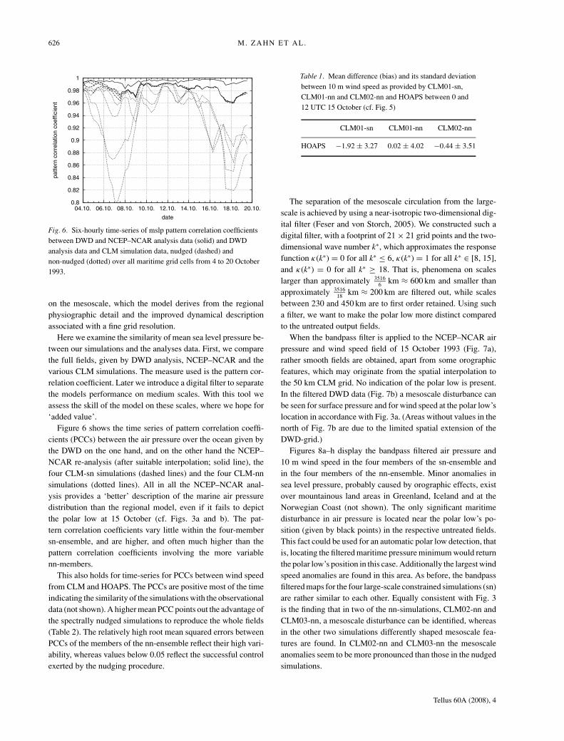
Fig. 5. Difference maps for 10 m wind speed as provided by CLM with spectral nudging (CLM01-sn) and without spectral nudging (CLM01-nn andCLM02-nn) compared to HOAPS-estimates on 15 October 1993, 0–12 UTC.

approximately 8 m s−1 occur over most of the polar low’s area.However, for the whole field a mean difference of −1.92 m s−1

was calculated. Such a mean difference is larger than the overallmean difference of −1.16 m s−1 calculated from 1 to 20 Oc-tober. Remarkably higher wind speeds in HOAPS in the polarlow’s area contribute to this discrepancy, whereas CLM01-snproduced higher wind speeds farther north-west, reflecting thesomewhat shifted position of the polar low in CLM01-sn. Thespatial standard deviation amounts to 3.27 m s−1, which is al-most one and a half as large as the spatial standard deviation ofthe difference field between HOAPS and DWD of 2.28 m s−1.

The differences between HOAPS and CLM-nn exceed 8 m s−1

in many parts of the area. The oval shaped synoptic low ofCLM01-nn, which is not seen in observations, was discussedabove. This low produces a large-scale high wind speed fieldto its western side leading to large positive differences withHOAPS (Fig. 5b). Contrary to CLM01-sn this leads to a no-tably smaller mean difference of 0.02 m s−1 between the twofields of CLM01-nn and HOAPS. Though a higher standarddeviation of 4.02 m s−1 indicates locally higher differences.For the CLM02-nn case a simulated polar low with a spatiallysomewhat larger extension delivers values in between, namely−0.44 ± 3.51 m s−1.

3.2. Scale separation

In this subsection, we expand the findings of the previous subsec-tion by focusing on the mesoscale features of the output fields.

Thereby we want to highlight a technique that might be help-ful for the automated detection of mesoscale disturbances bymaking them more distinct.

The retrospective simulation is based on the assumption thatthe limited area model provides additional detail on mesoscalesover the driving NCEP–NCAR re-analysis. Whether this expec-tation is valid is examined by comparing the performance ofthe retrospective simulation on the smaller scale with the 50 kmresolved DWD analysis, which is available only for a limitednumber of years (as opposed to NCEP–NCAR, which extendsback to the late 1940s). Thus, we consider the DWD analysis as‘truth’, that is, as a reference.

That this expectation is not groundless has already beendemonstrated by Feser and von Storch (2005), who examinedthe performance of another limited area model in terms of airpressure and near surface temperature. They found that the re-gional model fares worse for air pressure than the driving NCEP–NCAR analysis if spectral nudging is invoked on large-scales,but slightly better on mesoscales. This result is not surprising,as NCEP–NCAR has assimilated various local observations ofthe atmospheric mass distribution, which is dominated by large-scale features. Thus, the limited area model, which ‘knows’ lessabout reality than NCEP–NCAR, namely conditions along themargins and about the large-scale wind above 850 hPa, cannotfare better than the global re-analysis. However, it is reassuringthat in Feser’s results the slight deterioration in the descriptionof the large-scale is small enough to still harvest the added value

Tellus 60A (2008), 4

626 M. ZAHN ET AL.

0.8

0.82

0.84

0.86

0.88

0.9

0.92

0.94

0.96

0.98

1

04.10. 06.10. 08.10. 10.10. 12.10. 14.10. 16.10. 18.10. 20.10.

patte

rn c

orre

latio

n co

effic

ient

date

Fig. 6. Six-hourly time-series of mslp pattern correlation coefficientsbetween DWD and NCEP–NCAR analysis data (solid) and DWDanalysis data and CLM simulation data, nudged (dashed) andnon-nudged (dotted) over all maritime grid cells from 4 to 20 October1993.

on the mesoscale, which the model derives from the regionalphysiographic detail and the improved dynamical descriptionassociated with a fine grid resolution.

Here we examine the similarity of mean sea level pressure be-tween our simulations and the analyses data. First, we comparethe full fields, given by DWD analysis, NCEP–NCAR and thevarious CLM simulations. The measure used is the pattern cor-relation coefficient. Later we introduce a digital filter to separatethe models performance on medium scales. With this tool weassess the skill of the model on these scales, where we hope for‘added value’.

Figure 6 shows the time series of pattern correlation coeffi-cients (PCCs) between the air pressure over the ocean given bythe DWD on the one hand, and on the other hand the NCEP–NCAR re-analysis (after suitable interpolation; solid line), thefour CLM-sn simulations (dashed lines) and the four CLM-nnsimulations (dotted lines). All in all the NCEP–NCAR anal-ysis provides a ‘better’ description of the marine air pressuredistribution than the regional model, even if it fails to depictthe polar low at 15 October (cf. Figs. 3a and b). The pat-tern correlation coefficients vary little within the four-membersn-ensemble, and are higher, and often much higher than thepattern correlation coefficients involving the more variablenn-members.

This also holds for time-series for PCCs between wind speedfrom CLM and HOAPS. The PCCs are positive most of the timeindicating the similarity of the simulations with the observationaldata (not shown). A higher mean PCC points out the advantage ofthe spectrally nudged simulations to reproduce the whole fields(Table 2). The relatively high root mean squared errors betweenPCCs of the members of the nn-ensemble reflect their high vari-ability, whereas values below 0.05 reflect the successful controlexerted by the nudging procedure.

Table 1. Mean difference (bias) and its standard deviationbetween 10 m wind speed as provided by CLM01-sn,CLM01-nn and CLM02-nn and HOAPS between 0 and12 UTC 15 October (cf. Fig. 5)

CLM01-sn CLM01-nn CLM02-nn

HOAPS −1.92 ± 3.27 0.02 ± 4.02 −0.44 ± 3.51

The separation of the mesoscale circulation from the large-scale is achieved by using a near-isotropic two-dimensional dig-ital filter (Feser and von Storch, 2005). We constructed such adigital filter, with a footprint of 21 × 21 grid points and the two-dimensional wave number k∗, which approximates the responsefunction κ(k∗) = 0 for all k∗ ≤ 6, κ(k∗) = 1 for all k∗ ∈ [8, 15],and κ(k∗) = 0 for all k∗ ≥ 18. That is, phenomena on scaleslarger than approximately 3516

6 km ≈ 600 km and smaller thanapproximately 3516

18 km ≈ 200 km are filtered out, while scalesbetween 230 and 450 km are to first order retained. Using sucha filter, we want to make the polar low more distinct comparedto the untreated output fields.

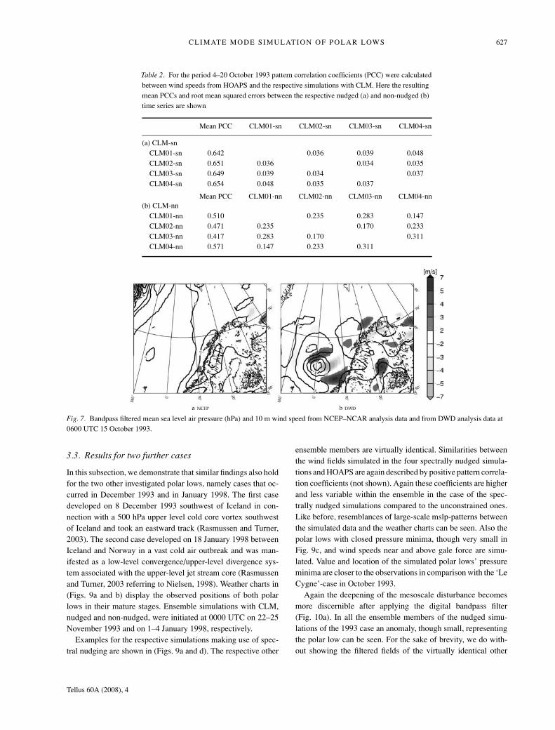
When the bandpass filter is applied to the NCEP–NCAR airpressure and wind speed field of 15 October 1993 (Fig. 7a),rather smooth fields are obtained, apart from some orographicfeatures, which may originate from the spatial interpolation tothe 50 km CLM grid. No indication of the polar low is present.In the filtered DWD data (Fig. 7b) a mesoscale disturbance canbe seen for surface pressure and for wind speed at the polar low’slocation in accordance with Fig. 3a. (Areas without values in thenorth of Fig. 7b are due to the limited spatial extension of theDWD-grid.)

Figures 8a–h display the bandpass filtered air pressure and10 m wind speed in the four members of the sn-ensemble andin the four members of the nn-ensemble. Minor anomalies insea level pressure, probably caused by orographic effects, existover mountainous land areas in Greenland, Iceland and at theNorwegian Coast (not shown). The only significant maritimedisturbance in air pressure is located near the polar low’s po-sition (given by black points) in the respective untreated fields.This fact could be used for an automatic polar low detection, thatis, locating the filtered maritime pressure minimum would returnthe polar low’s position in this case. Additionally the largest windspeed anomalies are found in this area. As before, the bandpassfiltered maps for the four large-scale constrained simulations (sn)are rather similar to each other. Equally consistent with Fig. 3is the finding that in two of the nn-simulations, CLM02-nn andCLM03-nn, a mesoscale disturbance can be identified, whereasin the other two simulations differently shaped mesoscale fea-tures are found. In CLM02-nn and CLM03-nn the mesoscaleanomalies seem to be more pronounced than those in the nudgedsimulations.

Tellus 60A (2008), 4

CLIMATE MODE SIMULATION OF POLAR LOWS 627

Table 2. For the period 4–20 October 1993 pattern correlation coefficients (PCC) were calculatedbetween wind speeds from HOAPS and the respective simulations with CLM. Here the resultingmean PCCs and root mean squared errors between the respective nudged (a) and non-nudged (b)time series are shown

Mean PCC CLM01-sn CLM02-sn CLM03-sn CLM04-sn

(a) CLM-snCLM01-sn 0.642 0.036 0.039 0.048CLM02-sn 0.651 0.036 0.034 0.035CLM03-sn 0.649 0.039 0.034 0.037CLM04-sn 0.654 0.048 0.035 0.037

Mean PCC CLM01-nn CLM02-nn CLM03-nn CLM04-nn(b) CLM-nn

CLM01-nn 0.510 0.235 0.283 0.147CLM02-nn 0.471 0.235 0.170 0.233CLM03-nn 0.417 0.283 0.170 0.311CLM04-nn 0.571 0.147 0.233 0.311

Fig. 7. Bandpass filtered mean sea level air pressure (hPa) and 10 m wind speed from NCEP–NCAR analysis data and from DWD analysis data at0600 UTC 15 October 1993.

3.3. Results for two further cases

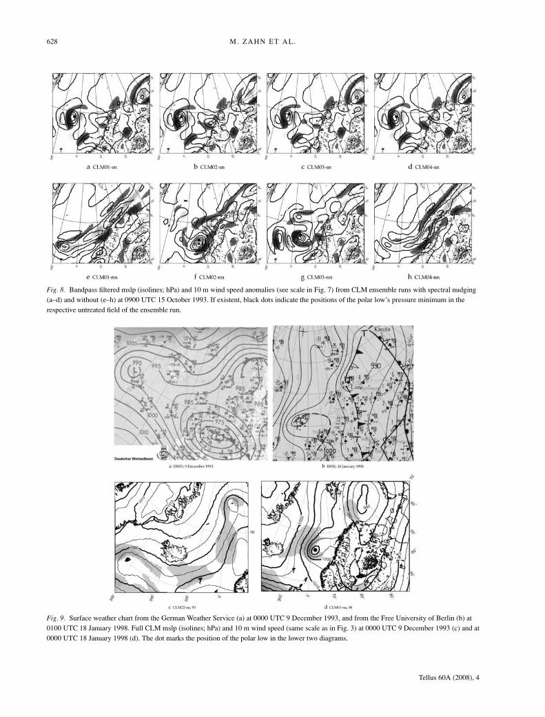
In this subsection, we demonstrate that similar findings also holdfor the two other investigated polar lows, namely cases that oc-curred in December 1993 and in January 1998. The first casedeveloped on 8 December 1993 southwest of Iceland in con-nection with a 500 hPa upper level cold core vortex southwestof Iceland and took an eastward track (Rasmussen and Turner,2003). The second case developed on 18 January 1998 betweenIceland and Norway in a vast cold air outbreak and was man-ifested as a low-level convergence/upper-level divergence sys-tem associated with the upper-level jet stream core (Rasmussenand Turner, 2003 referring to Nielsen, 1998). Weather charts in(Figs. 9a and b) display the observed positions of both polarlows in their mature stages. Ensemble simulations with CLM,nudged and non-nudged, were initiated at 0000 UTC on 22–25November 1993 and on 1–4 January 1998, respectively.

Examples for the respective simulations making use of spec-tral nudging are shown in (Figs. 9a and d). The respective other

ensemble members are virtually identical. Similarities betweenthe wind fields simulated in the four spectrally nudged simula-tions and HOAPS are again described by positive pattern correla-tion coefficients (not shown). Again these coefficients are higherand less variable within the ensemble in the case of the spec-trally nudged simulations compared to the unconstrained ones.Like before, resemblances of large-scale mslp-patterns betweenthe simulated data and the weather charts can be seen. Also thepolar lows with closed pressure minima, though very small inFig. 9c, and wind speeds near and above gale force are simu-lated. Value and location of the simulated polar lows’ pressureminima are closer to the observations in comparison with the ‘LeCygne’-case in October 1993.

Again the deepening of the mesoscale disturbance becomesmore discernible after applying the digital bandpass filter(Fig. 10a). In all the ensemble members of the nudged simu-lations of the 1993 case an anomaly, though small, representingthe polar low can be seen. For the sake of brevity, we do with-out showing the filtered fields of the virtually identical other

Tellus 60A (2008), 4

628 M. ZAHN ET AL.

Fig. 8. Bandpass filtered mslp (isolines; hPa) and 10 m wind speed anomalies (see scale in Fig. 7) from CLM ensemble runs with spectral nudging(a–d) and without (e–h) at 0900 UTC 15 October 1993. If existent, black dots indicate the positions of the polar low’s pressure minimum in therespective untreated field of the ensemble run.

Fig. 9. Surface weather chart from the German Weather Service (a) at 0000 UTC 9 December 1993, and from the Free University of Berlin (b) at0100 UTC 18 January 1998. Full CLM mslp (isolines; hPa) and 10 m wind speed (same scale as in Fig. 3) at 0000 UTC 9 December 1993 (c) and at0000 UTC 18 January 1998 (d). The dot marks the position of the polar low in the lower two diagrams.

Tellus 60A (2008), 4

CLIMATE MODE SIMULATION OF POLAR LOWS 629

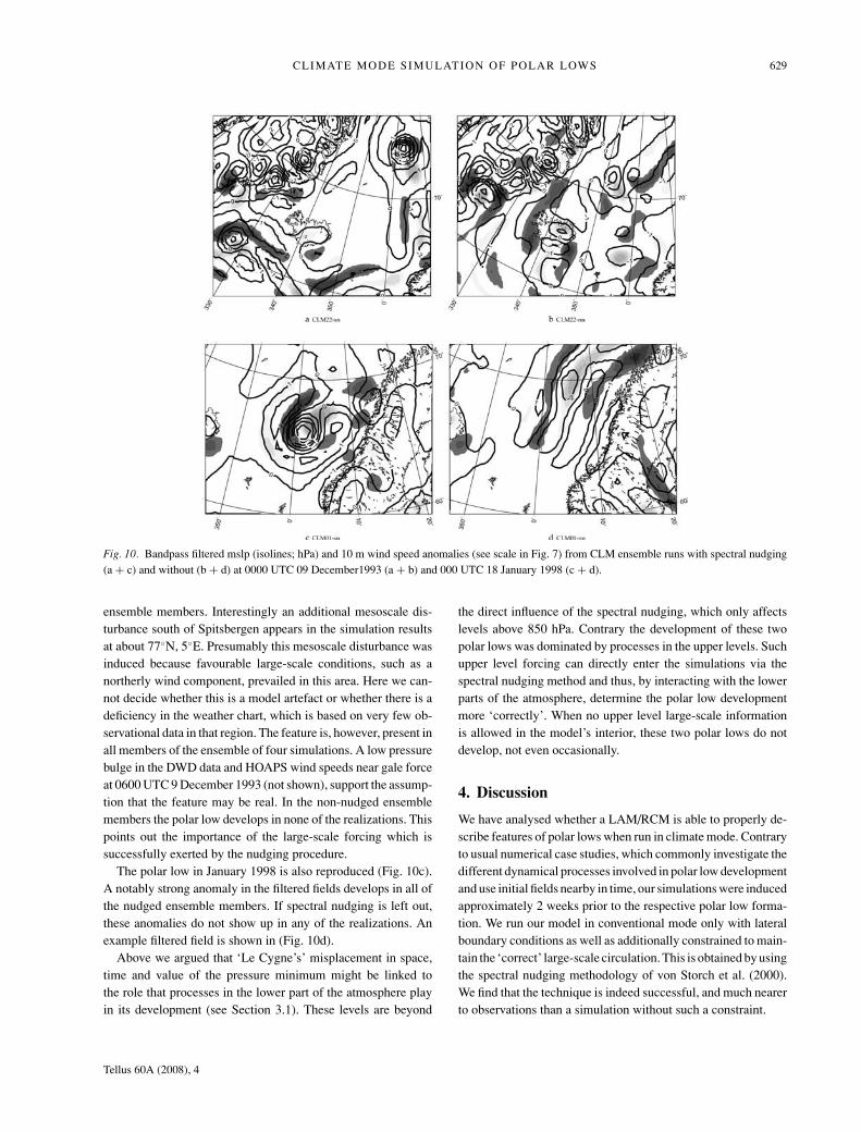
Fig. 10. Bandpass filtered mslp (isolines; hPa) and 10 m wind speed anomalies (see scale in Fig. 7) from CLM ensemble runs with spectral nudging(a + c) and without (b + d) at 0000 UTC 09 December1993 (a + b) and 000 UTC 18 January 1998 (c + d).

ensemble members. Interestingly an additional mesoscale dis-turbance south of Spitsbergen appears in the simulation resultsat about 77◦N, 5◦E. Presumably this mesoscale disturbance wasinduced because favourable large-scale conditions, such as anortherly wind component, prevailed in this area. Here we can-not decide whether this is a model artefact or whether there is adeficiency in the weather chart, which is based on very few ob-servational data in that region. The feature is, however, present inall members of the ensemble of four simulations. A low pressurebulge in the DWD data and HOAPS wind speeds near gale forceat 0600 UTC 9 December 1993 (not shown), support the assump-tion that the feature may be real. In the non-nudged ensemblemembers the polar low develops in none of the realizations. Thispoints out the importance of the large-scale forcing which issuccessfully exerted by the nudging procedure.

The polar low in January 1998 is also reproduced (Fig. 10c).A notably strong anomaly in the filtered fields develops in all ofthe nudged ensemble members. If spectral nudging is left out,these anomalies do not show up in any of the realizations. Anexample filtered field is shown in (Fig. 10d).

Above we argued that ‘Le Cygne’s’ misplacement in space,time and value of the pressure minimum might be linked tothe role that processes in the lower part of the atmosphere playin its development (see Section 3.1). These levels are beyond

the direct influence of the spectral nudging, which only affectslevels above 850 hPa. Contrary the development of these twopolar lows was dominated by processes in the upper levels. Suchupper level forcing can directly enter the simulations via thespectral nudging method and thus, by interacting with the lowerparts of the atmosphere, determine the polar low developmentmore ‘correctly’. When no upper level large-scale informationis allowed in the model’s interior, these two polar lows do notdevelop, not even occasionally.

4. Discussion

We have analysed whether a LAM/RCM is able to properly de-scribe features of polar lows when run in climate mode. Contraryto usual numerical case studies, which commonly investigate thedifferent dynamical processes involved in polar low developmentand use initial fields nearby in time, our simulations were inducedapproximately 2 weeks prior to the respective polar low forma-tion. We run our model in conventional mode only with lateralboundary conditions as well as additionally constrained to main-tain the ‘correct’ large-scale circulation. This is obtained by usingthe spectral nudging methodology of von Storch et al. (2000).We find that the technique is indeed successful, and much nearerto observations than a simulation without such a constraint.

Tellus 60A (2008), 4

630 M. ZAHN ET AL.

In the three cases considered and with the spectral nudg-ing procedure invoked, polar low development principally takesplace at about the right time and at about the right location.However for one polar low there are larger differences in detailbetween model and observations. For instance, the core pressureof the polar low in the simulation deviates from what obser-vational evidence points to. Also the location of the minimumpressure deviates by a distance of several 100 km in one case. Itseems that in conventional mode polar lows are only reproducedoccasionally.

We found signs that the spectral nudging procedure is partic-ularly successful for polar lows, which basically originate fromupper level disturbances. This is plausible because via the spec-tral nudging a large-scale closer to observations is enforced ontothe simulations. As a result more realistic and less random upperlevel fields are generated. Assuming a proper description of in-teractions between upper and lower levels in CLM, these morerealistic upper level fields in turn determine a more realistic polarlow development. Accordingly without spectral nudging, thesepolar lows did not develop at all. However, based on our few casesstudies, we cannot offer a statistically supported hypothesis.

In another study on the performance of spectrally nudged,multidecadal simulations, similar features were found. Eventswere simulated qualitatively correct, but deviations in detailshowed up. In this study more cases were available, so that thestatistics and not only the cases could be evaluated—and it turnedout that the deviations were not systematic and the statistics ofthe events were indeed well reproduced (Feser, 2006). We sug-gest that a similar situation may hold here. Of course at this timesuch a statement is a hypothesis, which needs to be tested in alarger ensemble of cases.

We applied a spatial digital bandpass filter to the simulatedoutput fields. In this way, the reproduced polar lows became moredistinct. We think that such a filter can be utilised in forthcominginvestigations on climatological aspects of polar low occurrencesin the North Atlantic. Such questions have been addressed byKolstad (2006) or Condron et al. (2006) before. However theywere not able to single out individual polar low occurrences.The minima in the bandpass filtered fields of a multidecadalsimulation might serve as a base for a detection algorithm. Ofcourse further constraints have to be applied. For instance, awind speed criterion should be implied. Also disturbances dueto orography have to be excluded. The definite constraints ofsuch a detection algorithm will have to be subject of furtherinvestigations. Then it might be possible to detect single polarlow occurrences in the output fields of multidecadal simulationsrun with spectral nudging invoked. Such a detection might serveas a base to investigate further climatological aspects of polarlows.

In a preliminary study we examined how another model,namely REMO (Zahn and von Storch, 2006) using a less suit-able region (Feser et al., 2001), was dealing with the formationof polar lows. These results are consistent with what we have

reported above. Therefore, we suggest that our results do notdepend on the specific model CLM used in this study We con-clude that important statistics of polar lows, such as frequencyof formation and tracks, may be described homogeneously byour method over several decades; thus assessments of recent,ongoing and possibly even future trends appear possible.

5. Acknowledgment

We are thankful to B. Rockel and B. Geyer for their help withthe model, to F. Feser for her help with the digital filter and to A.Andersson for providing the HOAPS-data. We are also thankfulto J. Winterfeldt and Tom Bracegirdle for reading the manuscript.The work was conducted within the Virtual Institute (VI)EXTROP which is promoted by the ‘Initiative and NetworkingFund’ of the Helmholtz Association.

References

Andersson, A., Bakan, S., Fennig, K., Grassl, H., Klepp, C.-P. and co-authors. 2007. Hamburg ocean atmosphere parameters and fluxes fromsatellite data—hoaps-3—twice daily composite. Electronic publica-tion: doi:10.1594/WDCC/HOAPS3 DAILY.

Blier, W. 1996. A numerical modeling investigation of a case of polarairstream cyclogenesis over the Gulf of Alaska. Mon. Wea. Rev. 124,2703–2725.

Bohm, U., Kucken, M., Ahrens, W., Block, A., Hauffe, D. and co-authors.2006. CLM - the climate version of LM: brief description and long-term applications. COSMO Newslett. 6, 225–235.

Bohm, U., Kucken, M., Hauffe, D., Gerstengarbe, F.-W., Werner, P.,Flechsig and co-authors. 2004. Reliability of regional climate modelsimulations of extremes and of long-term climate. Nat. Hazards EarthSyst. Sci. 4, 417–431.

Bracegirdle, T. J. and Gray, S. L. 2006. The Role of Convection in theIntensification of Polar Lows. PhD Thesis. The University of Reading,UK, 69 pp.

Bracegirdle, T. J. and Gray, S. L. 2008. An objective climatology of thedynamical forcing of polar lows in the Nordic seas. Int. J. Climatol.doi:10.1002/joc.1686.

Bresch, J. F., Reed, R. J. and Albright, M. D. 1997. A polar-low de-velopment over the Bering Sea: analysis, numerical simulation, andsensitivity experiments. Mon. Wea. Rev. 125, 3109–3130.

Carleton, A. M. and Carpenter, D. A. 1990. Satellite climatology of“polar lows” and broadscale climatic associations for the SouthernHemisphere. Int. J. Climatol. 10, 219–246.

Claud, C., Heinemann, G., Raustein. E. and Mcmurdie, L. 2004.Polar low ‘Le Cygne’: satellite observations and numerical simula-tions. Quart. J. Roy. Meteor. Soc. 130, 1075–1102.

Condron, A., Bigg, G. R. and Renfrew, I. A. 2006. Polar MesoscaleCyclones in the Northeast Atlantic: comparing Climatologies fromERA-40 and Satellite Imagery. Mon. Wea. Rev. 134, 1518–1533,doi:10.1175/MWR3136.1.

Davies, H. C. 1976. A lateral boundary formulation for multi-level pre-diction models. Quart. J. Roy. Meteorol. Soc. 102, 405–418.

Deque, M., Jones, R., Wold, M., Giorgi, F., Christensen, J. andco-authors. 2005. Global high resolution versus limited area

Tellus 60A (2008), 4

CLIMATE MODE SIMULATION OF POLAR LOWS 631

model climate change projections over Europe: quantifying confi-dence level from PRUDENCE results. Climate Dyn. 25, 653–670,doi:10.1007/s00382–005–0052–1.

Emanuel, K. A. 1986. An air-sea interaction theory for tropical cyclones.Part I: steady-state maintenance. J. Atmos. Sci. 43, 585–605.

Emanuel, K. A. and Rotunno, R. 1989. Polar lows as arctic hurricanes.Tellus 41A, 1–17.

Feser, F. 2006. Enhanced detectability of added value in limited areamodel results separated into different spatial scales. Mon. Wea. Rev.134, 2180–2190.

Feser, F. and von Storch, H. 2005. A spatial two-dimensional discretefilter for limited area model evaluation purposes. Mon. Wea. Rev. 133,1774–1786.

Feser, F., Weisse, R. and von Storch, H. 2001. Multi-decadal atmo-spheric modeling for Europe yields multi-purpose data. EOS Trans. 82,pp. 305, 310.

Grønas, S. and Kvamstø, N. 1995. Numerical simulations of the synopticconditions and development of arctic outbreak polar lows. Tellus 47A,797–814.

Harold, J. M., Bigg, G. R. and Turner, J. 1999a. Mesocyclone activitiesover the north-east Atlantic. Part 1: vortex distribution and variability.Int. J. Climatol. 19, 1187–1204.

Harold, J. M., Bigg, G. R. and Turner, J. 1999b. Mesocyclone activ-ities over the north-east Atlantic. Part 2: an investigation of causalmechanisms. Int. J. Climatol. 19, 1283–1299.

Harrold, T. W. and Browning, K. A. 1969. The polar low as a baroclinicdisturbance. Quart. J. Roy. Meteorol. Soc. 95, 710–723.

Heinemann, G. 1998. A meso-scale model-based study of the dynamicsof a wintertime polar low in the Weddell Sea region of the Antarcticduring WWSP86. J. Geophys. Res. 103, 5983–6000.

Heinemann, G. and Klein, T. 2003. Simulations of topographically forcedmesocyclones in the Weddell Sea and the Ross Sea region of Antarc-tica. Mon. Wea. Rev. 131, 302–316.

Kalnay, E., Kanamitsu, M., Kistler, R., Collins, W., Deaven, D. and co-authors. 1996. The NCEP/NCAR reanalysis project. Bull. Am. Mete-orol. Soc. 77, 437–471.

Kolstad, E. 2006. A new climatology of favourable conditions forreverse-shear polar lows. Tellus 58A, 344–354, doi:10.1111/j.1600–0870.2006.00171.x.

Lee, T.-Y., Park, Y.-Y. and Lin, Y.-L. 1998. A numerical modeling studyof mesoscale cyclogenesis to the east of the Korean Peninsula. Mon.Wea. Rev. 126, 2305–2329.

Mailhot, J., Hanley, D., Bilodeau, B. and Hertzman, O. 1996. A nu-merical case study of a polar low in the Labrador Sea. Tellus 48A,383–402.

Nielsen, N. W. 1997. An early Autumn polar low formation over theNorwegian Sea. J. Geophys. Res. 102, 13955–13973.

Nielsen, N. W. 1998. Om forudsigelighed af polare lavtryk (on the pre-dictability of polar lows). Vejret 20, 37–48. (In Danish).

Nordeng, T. and Rasmussen, E. 1991. A most beautiful polar low. A casestudy of a polar low development in the Bear Island region. Tellus 44A,81–99.

Rasmussen, E. 1979. The polar low as an extratropical CISK disturbance.Quart. J. Roy. Meteor. Soc. 105, 531–549.

Rasmussen, E. 1985. A case study of a polar low development over theBarents Sea. Tellus 37A, 407–418.

Rasmussen, E. and Turner, J. 2003. Polar Lows: Mesoscale WeatherSystems in the Polar Regions. Cambridge University Press,Cambridge.

Steppeler, J., Doms, G., Schattler, U., Bitzer, H., Gassmann, A. and co-authors. 2003. Meso-gamma scale forecasts using the nonhydrostaticmodel LM. Meteorol. Atmos. Phys. 82, 75–96.

von Storch, H., Langenberg, H. and Feser, F. 2000. A spectral nudgingtechnique for dynamical downscaling purposes. Mon. Wea. Rev. 128,3664–3673.

Weisse, R., von Storch, H. and Feser, F. 2005. Northeast Atlantic andNorth Sea storminess as simulated by a regional climate model 1958–2001 and comparison with observations. J. Climate 18, 465–479,doi:10.1175/JCLI–3281.1.

Wilhelmsen, K. 1985. Climatological study of gale-producing polar lowsnear Norway. Tellus 37A, 451–459.

Woth, K., Weisse, R. and von Storch, H. 2006. Climate change andnorth sea storm surge extremes: an ensemble study of storm surgeextremes expected in a changed climate projected by four differentregional climate models. Ocean Dyn. 56, 3–15, doi:10.1007/s10236–005–0024–3.

Yanase, W., Fu, G., Niino, H. and Kato, T. 2004. A polar low over theJapan Sea on 21 january 1997. Part II: a numerical study. Mon. Wea.Rev. 132, 1552–1574.

Yanase, W., Niino, H. and Saito, K. 2002. High-resolution numericalsimulation of a polar low. Geophys. Res. Lett. 29, 1658.

Zahn, M. and von Storch, H. 2006. Simulation of a Polar Low Case inthe North Atlantic with Different Regional Numerical Models. WGNEreport “Blue Book 2006”, 2pp.

Tellus 60A (2008), 4