Climate Change and Vulnerability to Poverty: An Empirical

ADBI Working Paper Series

CLIMATE CHANGE AND VULNERABILITY TO POVERTY: AN EMPIRICAL INVESTIGATION IN RURAL INDONESIA

Tomoki Fujii

No. 622 December 2016

Asian Development Bank Institute

The Working Paper series is a continuation of the formerly named Discussion Paper series; the numbering of the papers continued without interruption or change. ADBI’s working papers reflect initial ideas on a topic and are posted online for discussion. ADBI encourages readers to post their comments on the main page for each working paper (given in the citation below). Some working papers may develop into other forms of publication.

Suggested citation:

Fujii, T. 2016. Climate Change and Vulnerability to Poverty: An Empirical Investigation in Rural Indonesia. ADBI Working Paper 622. Tokyo: Asian Development Bank Institute. Available: https://www.adb.org/publications/climate-change-vulnerability-poverty-indonesia Please contact the authors for information about this paper.

Email: [email protected]

Tomoki Fujii is an associate professor of economics at Singapore Management University. The views expressed in this paper are the views of the author and do not necessarily reflect the views or policies of ADBI, ADB, its Board of Directors, or the governments they represent. ADBI does not guarantee the accuracy of the data included in this paper and accepts no responsibility for any consequences of their use. Terminology used may not necessarily be consistent with ADB official terms. Working papers are subject to formal revision and correction before they are finalized and considered published.

Asian Development Bank Institute Kasumigaseki Building, 8th Floor 3-2-5 Kasumigaseki, Chiyoda-ku Tokyo 100-6008, Japan Tel: +81-3-3593-5500 Fax: +81-3-3593-5571 URL: www.adbi.org E-mail: [email protected] © 2016 Asian Development Bank Institute

ADBI Working Paper 622 T. Fujii

Abstract Scientists estimate that anthropogenic climate change leads to increased surface temperature, sea-level rise, more frequent and significant extreme weather and climate events, among others. In this study, we investigate how climate change can potentially change the vulnerability to poverty using a panel data set in Indonesia. We focus on the effect of drought and flood, two of the commonly observed disasters there. Our simulation results indicate that vulnerability to poverty may increase substantially as a result of climate change in Indonesia. JEL Classification: I32, O10


Contents

1. INTRODUCTION ....................................................................................................... 1

2. CLIMATE CHANGE AND DISASTERS IN INDONESIA............................................. 2

Droughts .................................................................................................................... 3 Floods ........................................................................................................................ 4

3. DATA AND SUMMARY STATISTICS ........................................................................ 4

4. METHODOLOGY ...................................................................................................... 7

Measures of Vulnerability ........................................................................................... 7 Future Climate Scenarios and Simulations .............................................................. 10

5. EMPIRICAL RESULTS ............................................................................................ 10

Baseline Results ...................................................................................................... 10 Scenario 1(a): Doubling Incidence of Flood and Drought from IFLS 4...................... 12 Scenario 1(b): Special Treatment of Major ENSO Events ........................................ 14 Scenario 2: Using Linearly Extrapolated Standard Deviation of Daily Rainfall .......... 16

6. DISCUSSION .......................................................................................................... 17

REFERENCES ................................................................................................................... 20

APPENDIX: ADDITIONAL TABLES .................................................................................... 22


1. INTRODUCTION The impacts of climate change are multifarious and heterogeneous across the globe. Scientists now widely agree that climate change is likely to affect not only the average temperature of the earth’s surface but also various other dimensions, including agriculture, water resources, ecosystems, and prevalence of diseases. Climate change is also expected to affect frequency and magnitude of extreme weather and climate events, which, in turn, may alter the pattern of disasters such as floods and droughts. The way people are affected by these disasters may be different, even within relatively small areas, because some people are more resilient or adaptive. Those who are not resilient or adaptive may fall into poverty as a result of the negative shocks that disasters bring about. It is, therefore, important to understand who are vulnerable to extreme weather and climate events so that appropriate measures can be taken to minimize the negative shocks that these events bring about. However, despite the potential importance of these events, there is a dearth of research on climate-driven vulnerability to poverty. There are a few reasons for this. First, although there are some indications that the pattern of some extreme events has changed as a result of anthropogenic influences, including increases in atmospheric concentrations of greenhouse gases, there is a lack of clear scientific evidence that quality and quantity of extreme events have changed on regional and global scales for certain specific events. For example, the available instrumental records of floods at gauge stations are limited in space and time for a complete assessment of the climate-driven observed changes in the magnitude and frequency of floods at regional scales (IPCC 2012). This is also an important issue in Indonesia. Although the National Disaster Management Agency (Badan Nasional Penanggulangan Bencana) collects and maintains disaster information in Indonesia, the data are not directly comparable over time. For example, the number of recorded flood events is less than 15 each year between 1985 and 1997. However, the number of events after 2002 is over 100 every year between 2003 and 2013.1 This massive increase in the number of recorded flood events may be partly due to the actual increase in flood events, but it is most likely due to the better data collection in recent years. Second, the physical impact of extreme events may translate into different economic shocks to different households, even within the same town or village. Various factors, including the occupation of the household head, the household assets, the access to credit and insurance, and the local infrastructure development, are all likely to matter. However, socioeconomic surveys, from which poverty statistics are usually derived, typically contain no or very limited information about disasters and extreme events. Therefore, it is difficult to directly link poverty with extreme events. Despite these difficulties, given the observed increases in extreme events across the world, the topic is more relevant than ever before. The timeliness and increased importance of the climate-driven vulnerability to poverty can also be seen from the fact that the Fifth Assessment Report by the Intergovernmental Panel on Climate Change (IPCC) Working Group II, which traditionally focuses on adaptation and vulnerability, has a new chapter on “Livelihoods and Poverty” (IPCC 2014).

1 See also, http://dibi.bnpb.go.id/DesInventar/simple_data.jsp.

1


Because of the data availability and relevance, we focus on two common types of disasters in Indonesia, floods and droughts. We evaluate how these two types of disasters affect the vulnerability of households to poverty and simulate the impact of climate change on vulnerability to poverty under some plausible scenarios. This paper is organized as follows. In Section 2, we briefly present an overview of the situation of floods and droughts in Indonesia. In Section 3, we describe the data used, followed by a discussion of the method in Section 4. Section 5 presents the results and Section 6 offers some discussion.

2. CLIMATE CHANGE AND DISASTERS IN INDONESIA In Indonesia, various impacts of climate change have already been observed and are expected to take place. For example, modest temperature increase has already occurred and it is expected to continue. The rainy season is expected to shorten with more intense rainfall during the rainy season which, in turn, leads to a significant increase in the risk of flooding.2 Sea-level rise will inundate productive coastal zones and the warming of ocean water will affect the marine biodiversity. Climate change will also intensify water- and vector-borne diseases and threaten food security (PEACE 2007). Indonesia is among the first countries to experience the “climate departure”, which is the moment when the average temperature becomes so impacted by climate change that the old climate is left behind. It can be considered a tipping point such that the average temperature of the coolest year from then on is projected to be warmer than the average temperature of the hottest year between 1960 and 2005. Mora et al. (2013) estimate that Manokwari, Indonesia, is going to experience climate departure as early as 2020. Jakarta is estimated to have climate departure in 2029. These are substantially earlier than the world average of 2047 reported in the same study. The climate departure potentially will have a significant impact on the lives of people in Indonesia, the poor in particular, because there remain a sizable fraction of people who are either still under the poverty line or only slightly above the poverty line. For these people, the threat of poverty is far from over. If they are hit by a negative shock due to climate change, they may fall (further) below the poverty line. Therefore, Indonesia is a particularly important country to study in the context of climate-driven vulnerability to poverty. As mentioned earlier, we choose to focus on floods and droughts. We make this choice for two reasons. First, they are two of the most important impacts of climate change in Indonesia. Future climate change is likely to increase their frequency and severity in Indonesia. Second, floods and droughts are among the most commonly observed disasters. and, therefore, we have an accumulation of data on these types of disasters. Hence, we can arguably better predict whether climate change alters their frequency or incidence. In contrast, it is generally much more difficult to predict the impact of events that have never happened before. Just for the sake of comparison, consider coastal erosion induced by climate change. A substantial fraction of the population live close to the coast in Indonesia and they are sure to be negatively affected by sea-level rise; their lives as well as homes, lands, and other assets may become more vulnerable as a

2 The increasing trend in the standard deviation of daily rainfall presented later in Figure 1 is also indicative of the heightened risk of droughts and floods in the future.

2


result of climate change. However, this impact is difficult to predict because we have little information on how people would cope with coastal erosion.

Droughts

Droughts are common disasters in Indonesia, affecting some parts of Indonesia every year. Droughts negatively affect agricultural output and water supply. They are also associated with an increased incidence of forest fires. The incidence and magnitude of drought tend to be particularly higher during the phase of El Niño–Southern Oscillation (ENSO), which refers to the variations in the surface temperature of the tropical eastern Pacific Ocean and in air surface pressure in the tropical western Pacific. These variations happen because the trade winds, which carry wet and warm air from the west, tend to be weaker and, thus, dry and cold air tend to blow from the east during the El Niño years in Indonesia. This, in turn, tends to push back the onset of the rainy season as much as two months. As a result, ENSO tends to lead to droughts at the end of dry season. ENSO also tends to lead to floods during the rainy season because the rain tends to intensify during the rainy season.3 Using a model linking ENSO-based climate variability to Indonesian cereal production, Naylor et al. (2002) find, among others, that Indonesia’s paddy production varies, on average, by 1.4 million tonnes for every 1 ∘C change in sea-surface temperature anomalies—the deviation in temperature from a long-term monthly mean sea-surface temperature—for August. Droughts affect agricultural outputs because water is a key input for most agricultural outputs including rice, the main food crop grown in Indonesia. During El Niño years, widespread droughts affected 1-3 million hectares under paddy cultivation. Even during La Niña years, in which rainfall tends to be higher than average, localized droughts affect 30,000 to 80,000 hectares. On average, 280,000 hectares under paddy cultivation, which is much more than two percent of the total paddy area, are affected annually by drought to varying degrees. This means that nearly 160,000 farm households are vulnerable to these periodic droughts (Kishore et al. 2000). Droughts affect those farmers whose lives are dependent on their farmland. Based on regression analysis with cross-sectional data, Skoufias, Katayama and Essama-Nssah (2012) report a negative welfare impact of a significant shortfall in rain for farm households. Korkeala, Newhouse and Duarte (2009) find that a delayed onset of the monsoon season is associated with a 13 percent decline in per capita consumption for poor households but the delayed onset two years ago was positively correlated with consumption. This means that poor households experience greater volatility, but no lasting reduction in consumption, following delayed onset of the monsoon season. The findings of these studies indicate that drought mitigation measures may be useful. For example, Pattanayak and Kramer (2001a) measure the willingness to pay for drought mitigation from watershed protection in Ruteng Park in Indonesia by the Contingent Valuation Method. They find that farmers are willing to pay up to $2–3, which is about 10 percent of annual agricultural cost, 75 percent of the annual irrigation fees, and 3 percent of annual food expenditures. Pattanayak and Kramer (2001b) also reports a sizable benefit of drought mitigation based on a separate household model.

3 See, for example, Garrison (2010) for a general introductory discussion on ENSO events.

3


Floods

Floods are also common in Indonesia. For example, Jakarta has a long history of floods because of its geomorphology and intense seasonal rainfall. This problem has been exacerbated by rapid population growth, land-use change, waterways being clogged with household wastes and sediment from upstream. In recent years, massive floods were recorded in January 2002 and February 2007. There were, respectively, 57 and 70 deaths and 365,000 and 150,000 evacuees in these events. 4 In January 2014, 17.4 percent of Jakarta across 89 districts had been affected by a flood with 23 deaths and over 65,000 evacuees, according to the Jakarta Province Regionl Disaster Mitigation Agency (Badan Penanggulangan Bencana Daerah Provinsi DKI Jakarta). Floods also affect agricultural output. The order of magnitude of the impact of floods is comparable with that of droughts. For example, Hadi et al. (2000), cited by Pasaribu (2010), estimate that the sizes of paddy harvest failures due to floods and droughts are, respectively, 0.21 and 0.50 percent of the planted area during 1980–1998. According to the estimates by the Directorate General of Crop Protection, Ministry of Agriculture cited by Pasaribu (2010), the actual rice areas affected by floods and droughts are 333,000 and 319,000 hectares in 2008.

3. DATA AND SUMMARY STATISTICS The main data source for this study is the Indonesian Family Life Survey (IFLS), an on-going panel survey in Indonesia. The original sample frame covered 13 of the 27 provinces in Indonesia in 1993. Within each of these 13 provinces, enumeration areas were randomly drawn from a nationally representative sample frame used in the 1993 National Socio-Economic Survey (SUSENAS) designed by the Indonesian Central Bureau of Statistics (BPS). The sample was representative of about 83 percent of the Indonesian population in 1993. The first round of the IFLS (IFLS 1) was conducted in 1993/94 by the RAND Corporation, in collaboration with Lembaga Demografi, University of Indonesia. IFLS 2 was conducted in 1997, by the RAND Corporation, in collaboration with the University of California at Los Angeles and Lembaga Demografi, University of Indonesia.5 IFLS 3 was completed in 2000 and conducted by the RAND Corporation, in collaboration with the Population Research Center, University of Gadjah Mada. The IFLS 4 took place in 2007/08 and it was conducted by the RAND Corporation, the Center for Population and Policy Studies of the University of Gadjah Mada, and Survey METRE. In IFLS 1, a total of 7,224 households were interviewed and detailed individual-level data were collected from over 22,000 individuals. In IFLS 2, 94 percent of the IFLS 1 households and 91 percent of the IFLS 1 target individuals were re-interviewed. In IFLS 3, 95.3 percent of IFLS 1 households were re-contacted. In IFLS 4, the recontact rate was 93.6 percent. Among IFLS 1 dynasty households (any part of the original IFLS 1 households, 90.3 percent were either interviewed in all four waves or died, and 87.6 percent were actually interviewed in all four waves). These recontact rates are as high as or higher than most panel surveys in the United States and Europe. High reinterview rates were obtained, in part, because the data collection team was

4 “Your letters: Flooding in Jakarta–the facts”, Jakarta Post, January 28, 2014. 5 Additionally, IFLS 2+ was conducted in 1998, which covered a 25 percent sub-sample of the IFLS

households. IFLS 2+ is not used in this study.

4


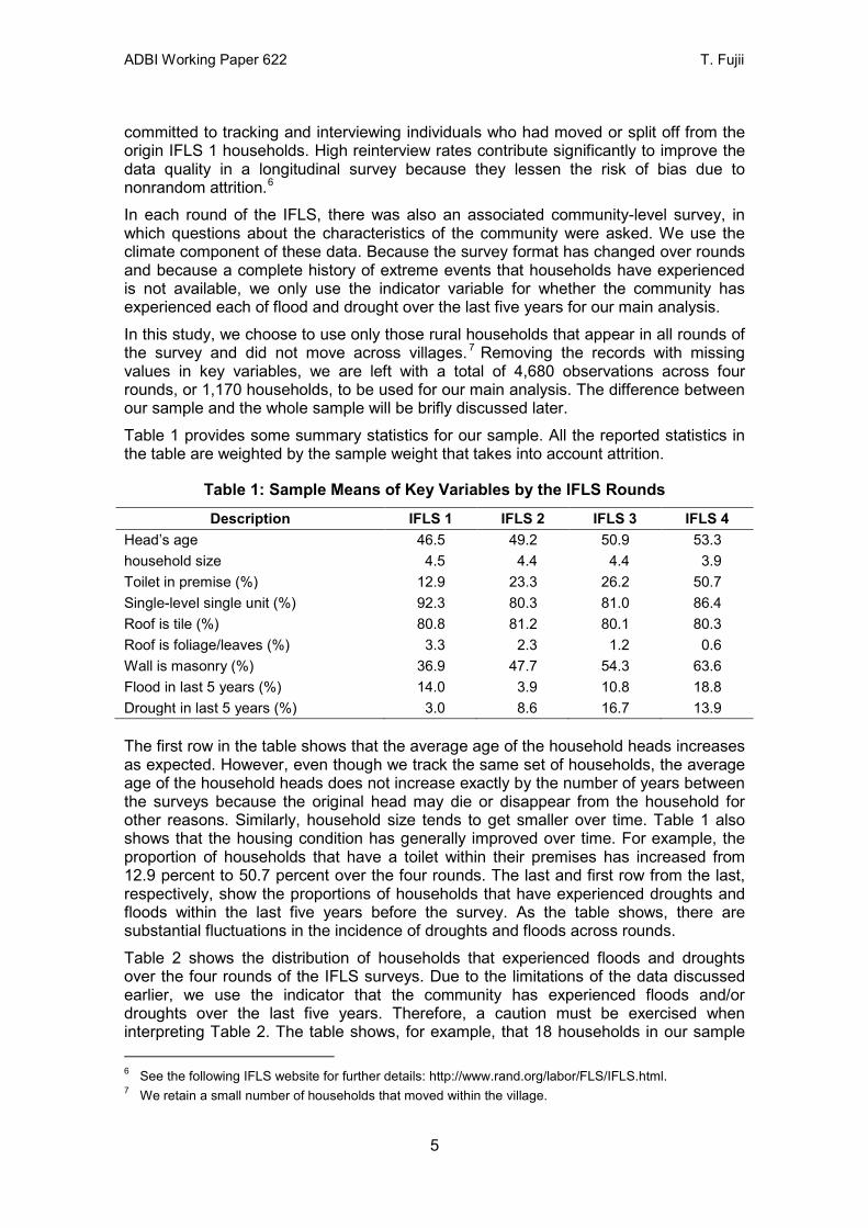
committed to tracking and interviewing individuals who had moved or split off from the origin IFLS 1 households. High reinterview rates contribute significantly to improve the data quality in a longitudinal survey because they lessen the risk of bias due to nonrandom attrition.6 In each round of the IFLS, there was also an associated community-level survey, in which questions about the characteristics of the community were asked. We use the climate component of these data. Because the survey format has changed over rounds and because a complete history of extreme events that households have experienced is not available, we only use the indicator variable for whether the community has experienced each of flood and drought over the last five years for our main analysis. In this study, we choose to use only those rural households that appear in all rounds of the survey and did not move across villages. 7 Removing the records with missing values in key variables, we are left with a total of 4,680 observations across four rounds, or 1,170 households, to be used for our main analysis. The difference between our sample and the whole sample will be brifly discussed later. Table 1 provides some summary statistics for our sample. All the reported statistics in the table are weighted by the sample weight that takes into account attrition.

Table 1: Sample Means of Key Variables by the IFLS Rounds Description IFLS 1 IFLS 2 IFLS 3 IFLS 4

Head’s age 46.5 49.2 50.9 53.3 household size 4.5 4.4 4.4 3.9 Toilet in premise (%) 12.9 23.3 26.2 50.7 Single-level single unit (%) 92.3 80.3 81.0 86.4 Roof is tile (%) 80.8 81.2 80.1 80.3 Roof is foliage/leaves (%) 3.3 2.3 1.2 0.6 Wall is masonry (%) 36.9 47.7 54.3 63.6 Flood in last 5 years (%) 14.0 3.9 10.8 18.8 Drought in last 5 years (%) 3.0 8.6 16.7 13.9

The first row in the table shows that the average age of the household heads increases as expected. However, even though we track the same set of households, the average age of the household heads does not increase exactly by the number of years between the surveys because the original head may die or disappear from the household for other reasons. Similarly, household size tends to get smaller over time. Table 1 also shows that the housing condition has generally improved over time. For example, the proportion of households that have a toilet within their premises has increased from 12.9 percent to 50.7 percent over the four rounds. The last and first row from the last, respectively, show the proportions of households that have experienced droughts and floods within the last five years before the survey. As the table shows, there are substantial fluctuations in the incidence of droughts and floods across rounds. Table 2 shows the distribution of households that experienced floods and droughts over the four rounds of the IFLS surveys. Due to the limitations of the data discussed earlier, we use the indicator that the community has experienced floods and/or droughts over the last five years. Therefore, a caution must be exercised when interpreting Table 2. The table shows, for example, that 18 households in our sample

6 See the following IFLS website for further details: http://www.rand.org/labor/FLS/IFLS.html. 7 We retain a small number of households that moved within the village.

5


experienced at least one drought within a period of five years before an IFLS survey for three rounds but no floods within a period of five years within any round of the IFLS surveys. Note that these households may have experienced droughts more than three times in our study period, because, for example, they may have experienced multiple droughts within five years before a particular round of the IFLS.

Table 2: The Numbers of Households that have Experienced Floods and Droughts in the IFLS Rounds

Drought

Flood 0 1 2 3 Total 0 486 127 67 18 698 1 241 25 71 0 337 2 38 74 23 0 135 Total 765 226 161 18 1,170

Because the floods and droughts are reported by the survey respondents and the way floods and droughts are reported across communities may not be strictly comparable, it is desirable to have an alternative measure of climate variations. To this end, we have compiled daily rainfall data at the provincial level.8 We then computed for each household the standard deviation in daily rainfall in the province the household belongs to over the past 365 days from the first interview for the household consumption module. We took this measure as a convenient measure of climate variability. This measure also has an advantage that the reference period is shorter than the flood and drought indicators taken from the IFLS data. However, because the rainfall are available only from 1997, the standard deviation over the last 365 days can be computed only from 1998. In Figure 1, we plot the standard deviation of provincial-level daily rainfall averaged over all the provinces for each year between 1997 and 2013. The dashed line represents the linear trend in the standard deviation of daily rainfall. We can see from this figure, that there is an increasing trend in the standard deviation of daily rainfall over the years involved. In this paper, we follow the standard consumption-based definition of poverty. To this end, we first define poverty lines. We consider the following three alternative sets of poverty lines: i) the official poverty lines, which are defined at the level of urban and rural areas annually;9 ii) the US$1.25-a-day international poverty line; and iii) the US$2-a-day international poverty line. For ii) and iii), we use the purchasing power parity conversion factor for private consumption in 2005 published in the World Development Indicators (USD 1=INR 4192.8) and adjust for the spatial price difference and inflation using the Consumer Price Index also available from the BPS website.10 Because the CPI data are only available for major cities, we use the CPI for the capital of the province in which the household was located.

8 We first obtain the provincial-level geographical coordinates from MyGeoPosition (http://mygeoposition .com/) and use these coordinates to obtain daily rainfall data from the agroclimatology data website by the Prediction of World Energy Resource, the National Aeronautics and Space Administration (http://power.larc.nasa.gov/cgi-bin/cgiwrap/solar/[email protected]).

9 They are available from the following website: http://www.bps.go.id/eng/tab_sub/view.php?kat=1 tabel =1 daftar=1 id_subyek=23 notab=7.

10 Obtained from http://www.bps.go.id/eng/aboutus.php?inflasi=1. Because the base year for the CPI changed over time, we link them by the CPI for the two contiguous months and the inflation rate reported in this website to cover our study period.

6


Figure 1: Standard Deviation of Daily Rainfall between 1997 and 2013

To measure poverty at the household level, we compare the total monthly consumption expenditure per capita, or the total monthly household expenditure divided by the household size, with the poverty line. If the consumption per capita of the household that the individual belonged to fell below the poverty line, the individual is deemed poor.

4. METHODOLOGY Measures of Vulnerability

As with most other studies in the literature, we define vulnerability to poverty 𝑉 as expected poverty. We denote the consumption per capita by 𝑐, the poverty line by 𝑧, their ratio by 𝑞� ≡ 𝑐/𝑧 . Further, we denote the censored ratio by 𝑞 = min(1,𝑞�) . We consider the following four vulnerability measures:

𝑉∞ = 𝐸[Ind(𝑞 < 1)]

𝑉1 = 𝐸[1 − 𝑞]

𝑉1/2 = 𝐸[1 − 𝑞1/2]

𝑉0 = −𝐸[ln𝑞],

where Ind(∙) is an indicator function that is equal to one when the argument is true and zero otherwise. The first measure is simply the expected headcount index and the most widely used measure in the literature including Chaudhuri, Jyotsna, and Suryahadi (2002). The second measure is the expected poverty-gap index. The third measure is the expected Chakravarty index with parameter 1/2. The fourth measure is the expected Watts measure. All these measures are an unscaled version of the measure proposed by Calvo and Dercon (2013).11 Although their parameter restriction would exclude 𝑉∞ and

11 Their measure is 𝑉𝐶𝐷𝑟 = 𝐸[(1 − 𝑞𝑟)/𝑟] for 𝑟 < 1 and 𝑟 ≠ 0 and 𝑉𝐶𝐷0 = −𝐸[ln𝑞].

7


𝑉1, we include them in this study because they have intuitive interpretations (they are respectively expected poverty rate and expected poverty gap). The former is also closely related to other vulnerability measures (See also Klasen and Povel (2013) and Fujii (2015a) for reviews of various vulnerability measures). To operationalize the expectations given above, we assume the following model of the ratio for each individual 𝑖 at time 𝑡:

ln𝑞�𝑖𝑡 = 𝑋𝑖𝑡𝑇𝛽 + 𝜀𝑖𝑡 , (1)

where 𝑋𝑖𝑡 is a column vector of values of covariates for ln𝑞�𝑖𝑡 ; and the idiosyncratic error term 𝜀𝑖𝑡 is assumed to be normally distributed with a zero mean but may be correlated across time or individuals. The error term 𝜀𝑖𝑡 is allowed to be

heteroskedastic and its standard deviation is given by 𝑠𝑖𝑡 ≡ �𝑉𝑎𝑟[𝜀𝑖𝑡] = �exp(𝑍𝑖𝑡𝑇𝜃),

where 𝑠𝑖𝑡 is a column vector of covariates for the variance of the idiosyncratic term. Although we set 𝑍𝑖𝑡 = 𝑋𝑖𝑡 in our empirical application as with various other empirical studies in the literature, 𝑍𝑖𝑡 and 𝑋𝑖𝑡 can be different, in general, and we maintain this difference in this section. Note that there are 1,170 individuals and 4 time periods. Hereafter, we focus on a particular individual in a particular period and drop subscripts 𝑖 and 𝑡 for most of the remainder of this section to keep the presentation simple. Given these assumptions, the vulnerability measures can be rewritten with the probability density function and the cumulative distribution function of normal distribution as the following proposition shows:

Proposition 1 Given the assumptions above, 𝑉∞ , 𝑉1 , 𝑉1/2 , and 𝑉0 can be written as follows:

𝑉∞ = Φ�−𝑋𝑇𝛽𝑠� (2)

𝑉1 = Φ�−𝑋𝑇𝛽𝑠� − exp �𝑋𝑇𝛽 + 𝑠2

2�Φ�−𝑋

𝑇𝛽𝑠

− 𝑠� (3)

𝑉1/2 = Φ�−𝑋𝑇𝛽𝑠� − exp �𝑋

𝑇𝛽2

+ 𝑠2

8�Φ�−𝑋

𝑇𝛽𝑠

− 𝑠2� (4)

𝑉0 = −𝑋𝑇𝛽Φ�−𝑋𝑇𝛽𝑠�+ 𝑠𝜙 �−𝑋

𝑇𝛽𝑠� (5)

Proof It is convenient to define the normalized error term by 𝑣 ≡ 𝜀/𝑠 . Then, eqs. (2)–(5) follow from below:

𝑉∞ = Pr(𝜀 < −𝑋𝑇𝛽) = Pr�𝑣 <−𝑋𝑇𝛽𝑠 �

𝑉1 = 𝐸[max(0,1− exp(𝑋𝑇𝛽 + 𝑠𝑣))]

= Φ�−𝑋𝑇𝛽𝑠 � − exp(𝑋𝑇𝛽)�

−𝑋𝑇𝛽𝑠

−∞exp(𝑠𝑣)𝑣𝜙(𝑣)𝑑𝑣

8


= Φ�−𝑋𝑇𝛽𝑠 � − exp�𝑋𝑇𝛽 +

𝑠2

2 �� −𝑋𝑇𝛽𝑠

−∞

exp �− (𝑣 − 𝑠)22 �

√2𝜋𝑑𝑣

𝑉1/2 = 𝐸[max(0,1−�exp(𝑋𝑇𝛽 + 𝑠𝑣))]

= Φ�−𝑋𝑇𝛽𝑠 � − exp�

𝑋𝑇𝛽2 ��

−𝑋𝑇𝛽𝑠

−∞exp �

𝑠𝑣2�𝜙(𝑣)𝑑𝑣

= Φ�−𝑋𝑇𝛽𝑠 � − exp�

𝑋𝑇𝛽2

+𝑠2

8 �� −𝑋𝑇𝛽𝑠

−∞

exp �− (𝑣 − 𝑠/2)22 �

√2𝜋𝑑𝑣

𝑉0 = 𝐸[max(0,−(𝑋𝑇𝛽 + 𝑠𝑣))]

= −𝑋𝑇𝛽Φ�−𝑋𝑇𝛽𝑠 � − 𝑠�

−𝑋𝑇𝛽𝑠

−∞𝑣𝜙(𝑣)𝑑𝑣,

where we use 𝜙′(𝑣) = −𝑣𝜙(𝑣) to obtain eq. (5).

As it can be seen from Proposition 1, both 𝑉1 and 𝑉1/2 have a very similar form. Their first terms are the same and represent the expected change in the extensive margin (i.e., whether the individual is below the poverty line). The differences in the second terms essentially come from the way the two measures treat the left tail in the consumption distribution.

To estimate these measures, we first obtain an estimate �̂� of the coefficient 𝛽 by ordinary least squares (OLS) regression. We then compute a logarithmic squared residual 𝑢 ≡ ln((ln𝑞� − 𝑋𝑇�̂�)2). By an OLS regression of 𝑢 on 𝑍, we obtain an estimate 𝜃�. Then, we obtain an estimate �̂�𝑖𝑡 of 𝑠𝑖𝑡 for each combination of (𝑖, 𝑡) as follows:

�̂�𝑖𝑡 = �exp�𝑍𝑖𝑡𝑇𝜃��

Replacing 𝛽 and 𝑠 by �̂� and �̂� in eqs. (2)–(5), we can estimate the vulnerability measures for each individual and each time period. In our empirical application, we assume that the vulnerability is the same for every member in the household. Therefore, we will aggregate household-level vulnerability by taking the average across households weighted by the population expansion factor, or the product of the household size and the household weight. It should be noted here that we run a linear regression of the logarithmic household consumption per capita over the poverty line on its covariates. This point is different from various other methods including that of Chaudhuri, Jyotsna, and Suryahadi (2002), which often involve estimating a binary regression of poverty status on its covariates. We chose a linear model because we can analytically derive various vulnerability measures in a coherent manner. This, in turn, has an added advantage that we are able to verify how our results are (in)sensitive to the choice of vulnerability measures.

9


Future Climate Scenarios and Simulations

Using the measures introduced above, we simulate the impact of climate change on vulnerability to poverty by changing the value of covariates. To operationalize this idea, we need some future climate scenarios. The main challenge here is that we do not yet know exactly how climate change would affect the lives of people through the channels of floods and droughts. In particular, scientists do not yet have enough evidence to establish a clear causal relationship between climate change and floods, even though they generally agree that anthropogenic climate change has increased and is likely to continue to increase the incidence of droughts and change the frequency and pattern of ENSO events. Therefore, we choose to adopt a few simple scenarios to present the possible order of magnitude of the impacts that future climate change may bring about. Our first scenario is the doubling incidence of floods and/or droughts from the 2007 (IFLS 4) level. This scenario is motivated by Cai et al. (2014), who predict that the frequency of major El Niño events may double in this century. Because El Niño events are related to floods and droughts, the doubling incidence of floods and droughts would not be completely unrealistic. However, because doubling incidence may appear extreme and the time horizon involved is very long, we also consider the case where the incidence of floods and/or droughts increases by 50 percent. As discussed in detail in the next section, we consider two cases under this scenario. In the first case (Scenario 1(a)), we treat all the floods and droughts observed in the IFLS data equally. In the second case (Scenario 1(b)), we assume that the droughts and floods in 1997 were different, because the ENSO event in 1997 is considered one of the largest in the observation history. As we shall show, there is some evidence that the ENSO event in 1997 was indeed different. Our second scenario (Scenario 2) is that the standard deviation of daily rainfall in a year at the provincial level changes linearly over time. In this exercise, we are, essentially, using the linear trend line similar to the one drawn in Figure 1 to predict the future standard deviation except that the trend line is defined for each province. Using a linear extrapolation to year 2030 for each province, we obtain the predicted standard deviation of daily rainfall. We then use this predicted value to compute the vulnerability to poverty under climate change. Although these scenarios are admittedly naïve, the results we present in the next section provide a plausible order of magnitude of the impact of climate change on vulnerability to poverty.

5. EMPIRICAL RESULTS Baseline Results

To compute the vulnerability measures, we first run regressions to estimate 𝛽 and 𝜃. Because the dependent variable in eq. (1) is ln𝑞�, which is the logarithm of consumption per capita normalized by the poverty line, the estimates depend not only on the consumption per capita but also on the poverty line. In Table 3, we report the baseline regression results when international poverty lines are used. In these regressions, we include the household-level fixed-effects terms to capture the unobserved heterogeneity across households. We also include IFLS-round-specific fixed-effects to absorb the aggregate shock to rural Indonesia in each round of the survey so that the changing macroeconomic environment is appropriately controlled for. In addition, we control for demographic characteristics of

10


households as well as our main variables of interest, indicator variables for floods and droughts experienced over the last five years in the community of residence. Note that the results presented in Table 3 are independent of whether we use $1.25 poverty line or $2 poverty line, because the constant term will absorb the difference. However, when the national poverty lines are used, the regression results are slightly different. This is because the national poverty lines are uniform within the rural areas each year whereas we adjust for the spatial price differences for the international poverty lines. In this section, we present the regression results based on international poverty lines only. The corresponding regression results based on national poverty lines are reported in Table A.1 in the Appendix.

As Table 3 shows, the flood variable has a negative 𝛽-coefficient, indicating that a flood tends to decrease the expected logarithmic consumption, though this coefficient is not significant. The 𝜃-coefficient on floods and droughts are both positive, suggesting that they tend to increase the variance of consumption, though the coefficient for floods is the only one that is significant.

Table 3: Regression Estimates of 𝜷 and 𝜽 for Scenario 1(a) 𝜷 𝜽

Variable Est. (s.e.) Est. (s.e.) Head’s age 0.018*** (0.0046) 0.00026 (0.022) Head’s age squared/100 –0.020*** (0.0043) –0.0063 (0.021) Household size –0.15*** (0.0066) –0.011 (0.031) Flood last five years –0.025 (0.024) 0.25** (0.12) Drought last five years 0.0067 (0.026) 0.14 (0.12) 𝑅2 0.6643 0.2893 N 4,680 4,680 Note: Household-specific and IFLS-round-specific fixed-effects terms are included in the model. International poverty lines are used for the calculation of 𝑞�. *, **, and ***, respectively, represent statistical significance at 10, 5, and 1 percent levels.

Table 4 presents various poverty and vulnerability measures for each round of the IFLS survey. All the results are weighted by the population expansion factor. In the first three rows, we report the Foster-Greer-Thorbecke (FGT) poverty measures (Foster, Greer and Thorbecke 1984) with parameters 𝛼 = 0, 𝛼 = 1, and 𝛼 = 2 for each round of IFLS survey, where the FGT measure with parameter 𝛼 is defined as follows:

𝐹𝐺𝑇𝛼 =1𝑁� 𝑖

Ind(𝑞𝑖 < 1)(1− 𝑞𝑖)𝛼 .

𝐹𝐺𝑇0 is simply the proportion of people who are under the poverty line and is often called the poverty rate or headcount index. Therefore, Table 4 shows, for example, that 53.8 percent of people in the IFLS 4 sample was living in a household whose consumption per capita was below the $2-a-day international poverty line. 𝐹𝐺𝑇1 is also called the poverty gap, which measures the average shortfall from the poverty line. 𝐹𝐺𝑇2 is called the poverty severity or the squared poverty gap and puts higher weights on the poorest of the poor. In the fourth and fifth rows, we respectively report the Watts poverty measure (Watts 1968) and the Chakravarty poverty measure (Chakravarty 1983) with parameter 𝜔 = 1/2, which are defined as follows:

11


𝑊 = −1𝑁� ln𝑞𝑖, 𝐶𝜔 =

1𝑁� 𝑖

(1 − 𝑞𝑖𝜔).

The Watts measure is the average logarithmic shortfall from the poverty line. As with 𝐹𝐺𝑇2, both the Watts and the Chakravarty measure put higher weight on the poorest of the poor. In all these measures, poverty has generally dropped over the four rounds of IFLS surveys, except that the poverty rate under the national poverty line has slightly increased between IFLS 2 and IFLS 3. Regardless of the poverty measure used, there is a substantial drop in poverty between IFLS 3 and IFLS 4, during which Indonesia achieved a healthy economic growth of around 4 percent per year in per capita income.

Table 4: Poverty Measures and Vulnerability Measures based on the Regression Reported in Tables 3 and A.1. Population Expansion Factor is Applied.

Poverty Line National Poverty Line

International Poverty Line $1.25

International Poverty Line $2

Round IFLS

1 IFLS

2 IFLS

3 IFLS

4 IFLS

1 IFLS

2 IFLS

3 IFLS

4 IFLS

1 IFLS

2 IFLS

3 ILFS

4 𝐹𝐺𝑇0 0.182 0.170 0.192 0.095 0.606 0.423 0.349 0.214 0.838 0.699 0.693 0.538 𝐹𝐺𝑇1 0.056 0.050 0.046 0.019 0.234 0.138 0.103 0.051 0.424 0.302 0.267 0.178 𝐹𝐺𝑇2 0.026 0.022 0.017 0.006 0.121 0.066 0.042 0.018 0.256 0.165 0.133 0.079 𝑊 0.079 0.068 0.058 0.024 0.351 0.198 0.136 0.065 0.694 0.463 0.384 0.242 𝐶1/2 0.033 0.029 0.026 0.011 0.141 0.082 0.059 0.029 0.265 0.184 0.158 0.103 𝑉∞ 0.145 0.135 0.173 0.097 0.619 0.397 0.354 0.218 0.857 0.718 0.686 0.537 𝑉1 0.038 0.034 0.044 0.022 0.218 0.117 0.099 0.055 0.422 0.289 0.264 0.178 𝑉1/2 0.021 0.019 0.025 0.013 0.128 0.067 0.057 0.031 0.260 0.172 0.157 0.104 𝑉0 0.049 0.044 0.058 0.028 0.308 0.158 0.133 0.072 0.661 0.423 0.380 0.247

The fifth to ninth rows are our vulnerability measures. To compute these, we plug the parameter values reported in Tables 3 or Table A.1 in the Appendix as well as the estimate of 𝑉 into eqs. (2)–(6). Because we have 𝑉∞ = 𝐸[𝐹𝐺𝑇0], 𝑉1 = 𝐸[𝐹𝐺𝑇1], 𝑉1/2 = 𝐸[𝐶1/2] , and 𝑉0 = 𝐸[𝑊] by definition, we expect to have 𝑉∞ ≃ 𝐹𝐺𝑇0 , 𝑉1 ≃𝐹𝐺𝑇1 , 𝑉1/2 ≃ 𝐶1/2 , and 𝑉0 ≃ 𝑊 , which indeed holds as shown in Table 4. As expected, the changes in our vulnerability measures have been similar to those of poverty measures.

Scenario 1(a): Doubling Incidence of Flood and Drought from IFLS 4

We now simulate how the vulnerability measures change as a result of future climate change. As discussed in Section 4, our first scenario is where the incidence of floods and droughts double from the 2007 level observed in IFLS 4. More precisely, 17.7 percent and 14.5 percent of the sample households experienced floods and droughts no more than five years from the IFLS 4 survey, respectively. We consider the effect of doubling these proportions. Because doubling may appear extreme and involves a long time horizon, we also consider 50 percent increase as a plausible change in the middle run.

12


A problem in this exercise is which households should bear the impact of floods and droughts in the future. Although it would not be impossible to estimate the floods and droughts risk for each household, we choose to assign floods and droughts randomly with an equal probability. We do this repeatedly under the assumption of independence between floods and droughts.12 That is, in each round of simulation, we randomly pick a predetermined number of households that are affected by floods or droughts. For these households, we change the values of 𝑋 and 𝑍 corresponding to floods or droughts in the computation of vulnerability while keeping all the other covariates and fixed-effects terms constant at the baseline level in 2007. We repeat this 1,000 times and take an average over all the rounds of simulation. The random assignment carried out in this way is not without problems. For the sake of argument, consider a situation in which only those households that are well above the poverty line are affected by floods and droughts. In this case, floods and droughts would not increase the vulnerability measures much, because the households that are hit by the disasters are likely to remain well above the poverty line. If we randomly assign floods and droughts without taking this pattern into consideration, the vulnerability would unambiguously increase, because the vulnerability measures for those household that are close or below the poverty line—assuming that we have such households—would worsen. In other words, the random assignment would increase the vulnerability measure. Hence, random assignment is not an innocuous exercise in general. It turns out that the pure effect of the random assignment is small in our data. The second column (“IFLS 4”) of Table 5 refers to the vulnerability measures for the IFLS 4 survey (they are the same as those reported in Table 4), which serve as our baseline measurement. In the third column (“Randomize”), we compute vulnerability measures by randomly and independently assigning floods and droughts without changing the total number of households that are affected by each of these disasters. Since there is little difference in these two columns, the random assignment has only negligible effect on the resulting vulnerability measure. The fourth column (1.5x Fl) of Table 5 shows the effect of increasing the incidence of floods by 50 percent. Compared with the third column, the vulnerability measure increases by around 2–3 percent (e.g., (0.100− 0.098)/0.098 ≃ 2% for 𝑉∞) when the national poverty line is used. The increase is even smaller when an international poverty line, especially the $2-a-day poverty line, is adopted. The fifth column (1.5x Dr) gives the effect of increasing the incidence of droughts by fifty percent. The change in vulnerability is generally smaller than those found for floods. The sixth column (1.5x Fl&Dr) gives the combined effect of the increase of incidence of both floods and droughts by 50 percent. The seventh, eighth, and ninth columns give the vulnerability measures when the incidence of flood, drought and both flood and drought double, respectively. As can be seen from the table, the impact of doubling the incidence is also small. The biggest relative change is seen in 𝑉0 under the national poverty line, but even in this case, the increase is only around 6 percent. Therefore, Table 5 shows that the combined impact of increased incidence of flood and drought is relatively small. The impact simulated here should be considered a long-run average and not a one-off impact as the flood and drought indicators used in this study are based on the incidence over the last five years.

12 It is also possible to assign floods and droughts jointly. However, we chose to maintain the independence assumption because the correlation between the flood and drought incidence is very small in our sample.

13


Table 5: Simulated Effects of Increasing the Incidence of Flood and Drought by 50 percent (1.5x) and 100 percent (2x) for Various Poverty Lines

under Scenario 1(a). Population Expansion Factor is Applied. Scenario IFLS 4 Randomize 1.5x Fl 1.5x Dr 1.5x Fl&Dr 2x Fl 2x Dr 2x Fl&Dr National Poverty Line 𝑉∞ 0.097 0.098 0.100 0.099 0.100 0.102 0.099 0.102 𝑉1 0.022 0.022 0.023 0.023 0.023 0.023 0.023 0.024 𝑉1/2 0.013 0.013 0.013 0.013 0.013 0.013 0.013 0.013 𝑉0 0.028 0.029 0.029 0.029 0.030 0.030 0.029 0.030 International Poverty Line $1.25 𝑉∞ 0.218 0.217 0.219 0.217 0.219 0.221 0.217 0.221 𝑉1 0.055 0.056 0.056 0.056 0.056 0.057 0.056 0.057 𝑉1/2 0.031 0.032 0.032 0.032 0.032 0.033 0.032 0.033 𝑉0 0.072 0.073 0.074 0.073 0.074 0.075 0.073 0.075 International Poverty Line $2 𝑉∞ 0.537 0.537 0.538 0.536 0.538 0.540 0.536 0.540 𝑉1 0.178 0.178 0.179 0.178 0.179 0.181 0.178 0.181 𝑉1/2 0.104 0.104 0.105 0.104 0.105 0.105 0.104 0.105 𝑉0 0.247 0.247 0.249 0.247 0.249 0.251 0.247 0.251

Scenario 1(b): Special Treatment of Major ENSO Events

Although an up to 7 percent increase in vulnerability (expected poverty) is not negligible, it may give a misleading impression about the importance of the impacts of flood and drought as the short-run effects may be severer. Hence, to simulate the possible magnitude of the short-run effects of major ENSO events, we utilize the fact that there was a major ENSO event right before the data collection of the IFLS2 survey Because this event was clearly a major one, it is reasonable to treat floods and droughts separately from those in other years. Table 6 reports the regression results under international poverty lines13 when the flood and drought effects are assumed to be different between IFLS 2 and other rounds of IFLS surveys. The table clearly shows that the order of magnitude of the effects of floods and droughts are different between IFLS 2 and other rounds. Unlike Table 3, the 𝛽-coefficients are statistically significant for both floods and droughts for IFLS 2, but not for other rounds of IFLS. Furthermore, we find that the major drought significantly increased the variance of consumption. It should be noted here that the vulnerability measures are generally model dependent. Therefore, the vulnerability measures reported in Table 4 are generally different from those calculated from the regression results reported in Table 6.

13 The regression results under the national poverty lines are reported in Table A.2 in the Appendix. As with Table 3, the regression results for $2 and $1.25 international poverty lines are identical except for the constant term.

14


Table 6: Regression Estimates of 𝜷 and 𝜽 for Scenario 1(b) 𝜷 𝜽

Variable Est. (s.e.) Est. (s.e.) Head’s age 0.019*** (0.005) 0.0082 (0.022) Head’s age squared/100 –0.020*** (0.004) –0.015 (0.021) Household size –0.15*** (0.007) –0.0050 (0.031) Flood last five years (non-IFLS2) –0.0015 (0.026) 0.32** (0.13) Drought last five years (non-IFLS2) 0.041 (0.030) 0.14 (0.14) Flood last five years (IFLS2) –0.21*** (0.071) –0.46 (0.34) Drought last five years (IFLS2) –0.073* (0.044) 0.36* (0.21) 𝑅2 0.6386 0.3014 N 4,680 5,584 Note: Household-specific and IFLS-round-specific fixed-effects terms are included in the model. International poverty lines are used for the calculation of 𝑞�. *, **, and *** respectively represent statistical significance at 10, 5, and 1 percent levels.

It should be noted here that the vulnerability measures are generally model dependent. Therefore, the vulnerability measures reported in Table 4 are generally different from those calculated from the regression results reported in Table 6. However, because the models are similar, the vulnerability measures are generally very close. 14As with Table 5, we report, in Table 7, the simulated effects of increased incidence of floods and droughts from the IFLS 4 level by 50 or 100 percent. However, unlike Scenario 1(a), the impacts of floods and droughts considered in Scenario 1(b) are those associated with a major ENSO event. Hence, we first replace the effects of flood and drought in IFLS 4 with those effects for 1997 (IFLS 2) without changing the flood or drought status in the IFLS 4 records. However, because the models are similar, the vulnerability measures are generally very close.15As with Table 5, we report, in Table 7, the simulated effects of increased incidence of floods and droughts from the IFLS 4 level by 50 or 100 percent. However, unlike Scenario 1(a), the impacts of floods and droughts considered in Scenario 1(b) are those associated with a major ENSO event. Hence, we first replace the effects of flood and drought in IFLS 4 with those effects for 1997 (IFLS 2) without changing the flood or drought status in the IFLS 4 records. By comparing the baseline vulnerability in the second column (IFLS 4) with the third column (1997-effect), it can be seen that simply replacing the effects of floods and droughts in 2007 (or non-IFLS 2) with those in 1997 (or IFLS 2) have a substantial impact on vulnerability. When the national poverty lines are used, there is about 40 percent increase in vulnerability, whereas the increase is around 20 and 10 percent when $1.25-a-day and $2-a-day poverty lines are used, respectively. The fourth column (Randomize) reports vulnerability measures when the assignment of floods and droughts are randomized. As with Table 5, the randomization has very little impact on the resulting vulnerability measures. The fifth column (1.5x Fl) reports the simulated vulnerability measures when the incidence of flood increases by 50 percent, where the impact of flood is equivalent to that observed in IFLS 2. Compared with the baseline vulnerability, the vulnerability has increased by well more than 50 percent in this case under the national poverty lines.

14 Round-by-round vulnerability measures for Scenario 1(b) are reported in Table A.4 in the Appendix.

15


Under international poverty lines, the relative change is about 11–28 percent, depending on the poverty line and vulnerability measure used. The impact of drought is less substantial than flood as shown in the sixth column (1.5x Dr) but the impact is still sizable. The combined effect is even more substantial as shown in the seventh column (1.5x Fl&Dr). Obviously, the impact is even larger when the incidence increases by 100 percent instead of 50 percent. The eighth to tenth columns report the vulnerability measures under the doubling incidence scenario. The combined effect of doubling the incidence of both floods and droughts is particularly large with the increase in vulnerability from the IFLS-4 baseline reaching as high as 91 percent.

Scenario 2: Using Linearly Extrapolated Standard Deviation of Daily Rainfall

In our second scenario, instead of the floods and droughts over the last five years, we use the standard deviation of daily provincial-level rainfall over the past 365 days counting from the first interview for the consumption component of the survey for each household. Table 8 reports the regression results with international poverty lines. 16 Note that the number of observations in this table is smaller because we can compute the standard deviation of daily rainfall only for IFLS 3 and IFLS 4 records.

Table 7: Simulated Effects of Increasing the Incidence of Flood and Drought by 50 percent (1.5x) and 100 percent (2x) for Various Poverty Lines under

Scenario 1(b). Population Expansion Factor is Applied. Scenario IFLS 4 1997-effect Randomize 1.5x Fl 1.5x Dr 1.5x Fl&Dr 2x Fl 2x Dr 2x Fl&Dr National Poverty Line 𝑉∞ 0.098 0.131 0.133 0.148 0.138 0.152 0.163 0.142 0.172 𝑉1 0.022 0.031 0.032 0.036 0.033 0.037 0.040 0.034 0.042 𝑉1/2 0.013 0.017 0.018 0.020 0.019 0.021 0.022 0.019 0.024 𝑉0 0.029 0.040 0.041 0.046 0.043 0.048 0.051 0.044 0.055 International Poverty Line $1.25 𝑉∞ 0.219 0.258 0.254 0.268 0.258 0.272 0.282 0.261 0.290 𝑉1 0.055 0.065 0.066 0.070 0.067 0.072 0.075 0.069 0.078 𝑉1/2 0.031 0.037 0.038 0.040 0.038 0.041 0.042 0.039 0.044 𝑉0 0.072 0.086 0.087 0.092 0.089 0.094 0.098 0.091 0.102 International Poverty Line $2 𝑉∞ 0.538 0.579 0.581 0.597 0.584 0.600 0.612 0.588 0.619 𝑉1 0.179 0.201 0.201 0.210 0.204 0.212 0.219 0.206 0.223 𝑉1/2 0.104 0.118 0.118 0.123 0.119 0.124 0.128 0.121 0.131 𝑉0 0.247 0.281 0.281 0.294 0.285 0.298 0.308 0.289 0.315

Table 8 shows that the 𝛽-coefficient on the standard deviation of daily rainfall over the past 365 days is negative and significant. The 𝜃-coefficient is also negative but it is not significant. To simulate the impact of climate change, we extrapolate the linear trend of provincial-level standard deviation in the annual rainfall to year 2030. To predict the future vulnerability in 2030, we replace the current standard deviation for IFLS 4 records with those extrapolated standard deviations. The results obtained in this way are provided in Table 9. For each set of poverty lines, we report the baseline vulnerability at IFLS 4

16 The regression results under national poverty lines are reported in Table A.3 in the Appendix.

16


and the predicted vulnerability in 2030. We observe about 2, 15, and 10 percent increase in vulnerability measures, respectively, when the national, $1.25-a-day, and $2-a-day poverty lines are used.

Table 8: Regression Estimates of 𝜷 and 𝜽 for Scenario 2 𝜷 𝜽

Variable Est. (s.e.) Est. (s.e.) Head’s age 0.017** (0.0074) –0.044* (0.024) Head’s age squared/100 –0.017** (0.0070) 0.041* (0.022) Household size –0.17*** (0.011) –0.0025 (0.028) SD of daily rainfall over the past 365 days –0.032* (0.017) –0.064 (0.044) 𝑅2 0.7675 0.0023 N 2,340 2,340 Note: Household-specific fixed-effects terms are included in the model. International poverty lines are used for the calculation of 𝑞�. *, **, and *** respectively represent statistical significance at 10, 5, and 1 percent levels.

Table 9: Vulnerability Measures under Scenario 2. Population Expansion Factor is Applied.

Poverty Line National International $1.25 International $2 Scenario IFLS 4 2030 IFLS 4 2030 IFLS 4 2030

𝑉∞ 0.105 0.107 0.247 0.285 0.579 0.623 𝑉1 0.020 0.021 0.057 0.068 0.194 0.218 𝑉1/2 0.011 0.011 0.032 0.038 0.112 0.126 𝑉0 0.025 0.025 0.071 0.086 0.263 0.299

6. DISCUSSION In this study, we consider the impact of climate change on vulnerability to poverty, defined as expected poverty, in rural Indonesia. We have considered two main scenarios. In the first scenario, we consider the case where future climate change doubles the incidence of floods and droughts. As an intermediary case, we also computed vulnerability when the incidence increases by 50 percent. Under this scenario, we computed the change in vulnerability for two cases, one case where the impact is estimated from flood and drought records over all the four rounds of the survey and the other case where the impact is derived essentially from the cross-sectional variations in year 1997, when a major ENSO event took place. Based on the former case, the increase in the vulnerability is modest and no greater than 7 percent for all the poverty lines and vulnerability measures considered in this study. However, for the latter case, doubling the flood and the drought incidences had a major impact on vulnerability. The increase in vulnerability was at least 15 percent and reached as high as 91 percent, depending on the vulnerability measure and poverty line used. Because the measurement of floods and droughts may not be strictly comparable, we also used rainfall data. By linearly extrapolating the standard deviation of daily rainfall over the last 365 days to year 2030, we predicted the vulnerability for year 2030. We found that there was a relatively large increase in vulnerability when $1.25-a-day international poverty line was used. The order of magnitude in this case is comparable

17


to the 50 percent increase in the incidence of both floods and droughts associated with a major ENSO event (Scenario 1(b)). There are a few important limitations in this study. First, our climate scenarios and simulation method are admittedly rudimentary. For example, we chose a random assignment for the sake of simplicity and tractability. Because the effect of random assignment is small in our sample, we do not have any evidence to indicate that our prediction is seriously biased due to the random assignment. However, this does not exclude the possibility that the future climate change systematically affects certain types of people more than others. Second, we only consider the impacts of floods and droughts. Other important changes such as sea-level rises are ignored. Therefore, our estimates are likely to underestimate the overall effect of climate change on vulnerability to poverty. Third, our measures of vulnerability are all individual-level vulnerability averaged over the sample. That is, our vulnerability measures are additively separable across individuals. However, it could be argued that the society is more vulnerable if a bad shock simultaneously affects everyone once it happens. To take this perspective into consideration, it is possible, for example, to use the social vulnerability measure proposed by Calvo and Dercon (2013). A practical difficulty, though, is that we need to know the current and future correlation of floods and droughts across households. Because our understanding of the impact of climate change through floods and droughts, especially flood, is limited, we chose to leave this as an exercise for future research. Fourth, the current analysis ignores the general equilibrium effects. To see this issue, suppose that various parts of Indonesia or even various parts of the world including Indonesia are hit simultaneously by correlated climate shocks (not necessary hit by the same flood or drought). Then, the impact on the household would be different from what it would be without such correlated climate shocks. This is because, for example, such correlated shocks would affect the relative prices, whereas an idiosyncratic shock for a particular household or a community would have a negligible impact on relative prices. Fifth, we do not take into account the possibility of non-linearity of the impact, even though it is potentially important. For example, once climate departure occurs, the nature of the impacts of an ENSO event may change systematically and non-linearly. Similarly, when we extrapolate the impact with the standard deviation of rainfall, we assumed that the impact would increase linearly with the standard deviation but this may not hold even in approximation. Further scientific research will be needed to fully address these issues. Finally, the estimates we provide are based on the condition that the households stay in the same village throughout our observation periods. This is a stringent restriction especially given that those households which can no longer survive in the same village will have to move. However, we chose to restrict our sample to control for a variety of unobservable factors that are specific to the location of residence with fixed-effects terms. Although we cannot draw strong conclusions, we can find the nature of households we used by comparing summary statistics in Tables A.5 and A.6 in the Appendix with Tables 1 and 2. The comparison appears to indicate that the general housing conditions at the beginning of the survey in our sample were slightly better than the average for the whole sample, which may be because those living in a poorly-built

18


house are more likely to move when they are hit by a disaster. On the other hand, the incidences of floods and droughts do not appear to be drastically different. Given the limitations above, it appears likely that our estimates provide a plausible lower-bound of the impact of future climate change on vulnerability. Although the long-run effects of floods and droughts appear rather limited, the short-run effects are sizable. Besides providing some plausible estimates of the impact of future climate change on vulnerability to poverty in Indonesia, this study contributes to the existing literature in several ways. First, to the best of our knowledge, this is the first study to directly link climate change with vulnerability to poverty using panel data. This is an important first step because most of the existing studies on the impact of climate change rely heavily on global climate models and do not take into account the standards of living observed in household surveys. Although there have been a few exceptions such as Adger (1999), they are based on cross-sectional evidence and thus require much stronger assumptions than ours. Further, they do not provide any estimates on the possible impact of future climate change. Second, we also make a methodological contribution by proposing a variant of the expected poverty approach that bridges the popular measure of expected poverty rate by Chaudhuri, Jyotsna, and Suryahadi (2002) and the axiomatically-derived vulnerability measure by Calvo and Dercon (2013). We offer a practical method in which various vulnerability measures can be computed in a coherent manner. The methodology used in this study can be applied easily to other countries if a relevant panel data set is available. This study also underscores the importance of monitoring the economic situation of households in developing countries that are likely to be affected by climate change because current global climate models do not tell us how climate change affects vulnerability to poverty. By linking global climate models with household-based observations, we will be able to make more meaningful prediction about the possible impacts of future climate changes on households including vulnerability to poverty.

19


REFERENCES Adger, N. 1999. Social Vulnerability to Climate Change and Extremes in Coastal

Vietnam. World Development 27(2): 249–269. Cai, W., S. Borlace, M. Lengaigne, P. van Rensch, M. Collins, G. Vecchi,

A. Timmermann, et al. 2014. Increasing Frequency of Extreme El Niño Events due to Greenhouse Warming. Nature Climate Change 4: 111–116.

Calvo, C., and S. Dercon. 2013. Vulnerability of Individual and Aggregate Poverty. Social Choice and Welfare 41: 721–740.

Chakravarty, S.R. 1983. A New Index of Poverty. Mathematical Social Sciences 6: 307–313.

Chaudhuri, S., J. Jyotsna, and A. Suryahadi. 2002. Assessing Household Vulnerability to Poverty from Cross-sectional Data: A Methodology and Estimates from Indonesia. Discussion Paper Series 0102-52, Department of Economics, Columbia University.

Foster, J., J. Greer, and E. Thorbecke. 1984. A Class of Decomposable Poverty Measures. Econometrica 52(3): 761–766.

Fujii, T. 2015a. Concepts and Measurement of Vulnerability to Poverty and Other Issues: A Review of Literature. ADBI Working Papers (to appear).

———. 2015b. Climate Change and Vulnerability to Poverty: An Empirical Investigation in Rural Indonesia. ADBI Working Papers (to appear).

Garrison, T.S. 2010. Oceanography: An Invitation to Marine Science, Seventh Edition. Cengage Learning.

Glantz, M.H. 2001. Executive Summary: Reducing the Impact of Environmental Emergencies through Early Warning and Preparedness: The Case of the 1997-98 El Niño. A UNEP/NCAR/UNU/WMO/ISDR Assessment, United Nations Environment Programme, National Center for Atmospheric Research, World Meteorological Organization, United Nations University, and International Strategy for Disaster Reduction, January

Hadi, P.U., C. Saleh, A.S. Bagyo, Hendayana R., Y. Marisa, and I. Sadikin. 2000. Studi kebutuhan asuransi pertanian pada pertanian rakyat.’ Research Report, Indonesian Center for Agricultural Socio-economic Research, Bogor, Indonesia.

IPCC. 2012. Managing the Risks of Extreme Events and Disasters to Advance Climate Change Adaption: A Special Report of Working Groups I and II of the Intergovernmental Panel on Climate Change, edited by Field, C.B., V. Barros, T.F. Stocker, D. Qin, D.J. Dokken, K.L. Ebi, M.D. Manstrandrea, et al. Cambridge, UK and New York, NY, USA: Cambridge University Press.

———. 2014. Climate Change 2014: Impacts, Adaptation, and Vulnerability. Part A: Global and Sectoral Aspects. Contribution of Working Group II to the Fifth Assessment Report of the Intergovernmental Panel on Climate Change, edited by Field, C.B., V.R. Barros, D.J. Dokken, K.J. Mach, M.D. Mastrandrea, T.E. Bilir, M. Chatterjee, et al. Cambridge, UK and New York, NY, USA: Cambridge University Press.

Kishore, K., A.R. Subbiah, T. Sribimawati, I.S. Dihart, S. Alimoeso, P. Rogers, and D. Setiana. 2000. Indonesia Country Study. In Glantz (2001: 103–109), Asian Disaster Preparedness Center.

20


Klasen, S., and F. Povel. 2013. Defining and Measuring Vulnerability: State of the Art and New Proposals. In Vulnerability to Poverty: Theory, Measurement and Determinants, edited by S. Klasen and H. Waibel, Palgrave-Macmillan.

Korkeala, O., D. Newhouse, and M. Duarte. 2009. Distributional Impact Analysis of Past Climate Variability in Rural Indonesia. World Bank Policy Research Working Paper 5070, World Bank.

Mora, C., A.G. Frazier, R.J. Longman, R.S. Dacks, M.M. Walton, E.J. Tong, J.J. Sanchez, et al. 2013. The Projected Timing of Climate Departure from Recent Variability. Nature 502: 183–187.

Naylor, R., W. Falcon, N. Wada, and D. Rochberg. 2002. Using El Niño-Southern Oscillation Climate Data to Improve Food Policy Planning in Indonesia. Bulletin of Indonesian Economic Studies 38(1): 75–91.

Pasaribu, S.M. 2010. Developing Rice Farm Insurance in Indonesia. Agriculture and Agricultural Science Procedia 1: 33–41.

Pattanayak, S.K., and R.A. Kramer. 2001a. Pricing Ecological Services: Willingness to Pay for Drought Mitigation from Watershed Protection in Eastern Indonesia. Water Resources Research 37(3): 771–778.

———. 2001b. Worth of Watersheds: A Producer Surplus Approach for Valuing Drought Mitigation in Eastern Indonesia. Environmental and Development Economics 6: 123–146.

PEACE. 2007. Indonesia and Climate Change: Current Status and Policies. Jakarta, Indonesia: World Bank, Department for International Development, and PT Pelangi Energi Abadi Citra Enviro.

Skoufias, E., R.S. Katayama, and B. Essama-Nssah. 2012. Too Little Too Late: Welfare Impacts of Rainfall Shocks in Rural Indonesia. Bulletin of Indonesian Economic Studies 48(3): 351–368.

Watts, H.W. 1968. An Economic Definition of Poverty. In On Understanding Poverty, edited by D.P. Moynihan. New York: Basic Books, 316–329.

21


APPENDIX: ADDITIONAL TABLES Table A.1: Regression Estimates of 𝜷 and 𝜽 for Scenario 1(a).

𝜷 𝜽 Variable Est. (s.e.) Est. (s.e.)

Head’s age 0.019*** (0.0046) 0.024 (0.022) Head’s age squared/100 –0.020*** (0.0043) –0.029 (0.020) Household size –0.15*** (0.0066) –0.028 (0.031) Flood last five years –0.036 (0.024) 0.22* (0.11) Drought last five years –0.0049 (0.026) 0.185 (0.12) 𝑅2 0.6359 0.2936 N 4,680 4,680 Note: Household-specific and IFLS-round-specific fixed-effects terms are included in the model. National poverty lines are used for the calculation of 𝑞� . *, **, and *** respectively represent statistical significance at 10, 5, and 1 percent levels.

Table A.2: Regression Estimates of 𝜷 and 𝜽 for Scenario 1(b) 𝜷 𝜽

Variable Est. (s.e.) Est. (s.e.) Head’s age 0.019*** (0.0046) 0.021 (0.021) Head’s age squared/100 –0.021*** (0.0043) –0.022 (0.020) Household size –0.16*** (0.0065) –0.020 (0.031) Flood last five years (non-IFLS2) –0.0031 (0.026) 0.39*** (0.12) Drought last five years (non-IFLS2) 0.048 (0.030) 0.20 (0.14) Flood last five years (IFLS2) –0.31*** (0.070) –0.30 (0.33) Drought last five years (IFLS2) –0.13*** (0.044) 0.32 (0.21) 𝑅2 0.6386 0.3014 N 4,680 5,584 Note: Household-specific and IFLS-round-specific fixed-effects terms are included in the model. National poverty lines are used for the calculation of 𝑞� . *, **, and *** respectively represent statistical significance at 10, 5, and 1 percent levels.

Table A.3: Regression Estimates of 𝜷 and 𝜽 for Scenario 2 𝜷 𝜽

Variable Est. (s.e.) Est. (s.e.) Head’s age 0.018** (0.0074) –0.061** (0.024) Head’s age squared/100 –0.018** (0.0069) 0.058*** (0.022) Household size –0.17*** (0.011) –0.019 (0.028) SD of daily rainfall over the past 365 days –0.0049 (0.017) –0.074 (0.045) 𝑅2 0.7692 0.0023 N 2,340 2,340 Note: Household-specific fixed-effects terms are included in the model. National poverty lines are used for the calculation of 𝑞�. *, **, and *** respectively represent statistical significance at 10, 5, and 1 percent levels.

22


Table A.4: Vulnerability Measures based on the Regression Reported in Tables 6 and A.2. Population Expansion Factor is Applied.

Poverty Line National Poverty Line

International Poverty Line $1.25

International Poverty Line $2

Round IFLS

1 IFLS

2 IFLS

3 ILFS

4 IFLS

1 IFLS

2 IFLS

3 ILFS

4 IFLS

1 IFLS

2 IFLS

3 ILFS

4 𝑉∞ 0.147 0.135 0.173 0.098 0.621 0.395 0.355 0.219 0.857 0.712 0.687 0.538 𝑉1 0.038 0.034 0.043 0.022 0.219 0.116 0.099 0.055 0.423 0.287 0.265 0.179 𝑉1/2 0.022 0.019 0.025 0.013 0.129 0.067 0.057 0.031 0.260 0.171 0.157 0.104 𝑉0 0.051 0.044 0.057 0.029 0.309 0.157 0.134 0.072 0.663 0.420 0.381 0.247

Table A.5: Sample Means of Key Variables for the Whole Sample Description IFLS 1 IFLS 2 IFLS 3 IFLS 4

Head’s age 46.2 48.7 48.2 47.9 household size 4.5 4.5 4.3 3.9 Toilet in premise (%) 25.2 36.5 39.5 57.6 Single-level single unit (%) 87.1 78.8 77.8 80.9 Roof is tile (%) 76.4 76.0 78.2 76.5 Roof is foliage/leaves (%) 4.2 2.2 1.9 1.2 Wall is masonry (%) 47.1 57.2 62.0 72.0 Flood last five years (%) 15.7 13.7 15.9 23.6 Drought last five years (%) 1.7 9.7 9.7 12.0

Table A.6: The Number of Households that have Experienced Floods and Droughts for the Whole Sample

Drought Flood 0 1 2 3 Total

0 5,543 735 206 34 6,518 1 2,063 253 201 0 2,517 2 558 159 23 0 740 3 209 0 0 0 209 4 19 0 0 0 19 Total 8,392 1,147 430 34 10,003

23

Documents

Climate Change and Vulnerability to Poverty: An Empirical