CLIMATE CHANGE AND LAND USE PATTERN IN BRAZIL

CLIMATE CHANGE AND LAND USE PATTERN IN BRAZIL

Eduardo Barbosa

José Féres

Eduardo A. Haddad

Antonio Paez

TD Nereus 12-2012

São Paulo

2012

1

Climate Change and Land Use Pattern in Brazil1

E. Barbosa, J. Feres, E. Haddad, and A. Paez

Abstract. The objective of this dissertation is to assess the impacts of climate change on

the land use pattern in Brazil. To do so an economic model for optimal land use

allocation was used. This model was derived from the profit maximization problem of a

representative agent that has six options of land use: soybean, corn, sugar cane, other

crops, pasture land and forests. From the estimated coefficients of the model

simulations were carried using forecast data for temperature and precipitation in three

periods of times 2010-39, 2040-69 and 2070-99. The results varied greatly in different

regions but in general the area for pasture land increased while the areas for forests

declined.

1. Introduction

In recent years there is an increasing concern among the different segments of society

with the possible economic and social impacts of climate changes. Evidence indicates

that higher green gas concentrations in the atmosphere will have a significant effect on

the planet. Therefore, the possible economic impacts of climate changes have been the

subject of academic debate, and the study of such impacts, both globally and regionally,

is essential to the understanding of the problem and its consequences.

There is a common understanding that climate changes would impact several economic

sectors. Analysis of agricultural and livestock farming is important for understanding

the economic impacts of climate changes in the different regions of the globe, for this

sector is directly affected by changes in temperature and rainfall.

In Brazil, the agricultural sector contributes to a large share of the national exports,

having accounted for 37.9% of exports in 2010. It is of great importance because it has

helped to ensure the macroeconomic stability and balance of payments equilibrium

observed in Brazil in the last decade. Moreover, in the context of climate change, the

agricultural sector plays a major role in the country because high levels of carbon

dioxide (CO2) emissions come from this sector.

1 This paper is based on the results of Barbosa’s M.A. thesis, defended at the Department of Economics at

the University of São Paulo. Haddad has acted as his thesis adviser and Féres as his co-adviser; Paez also

acted as his co-adviser during his visit at MacMaster University, when part of the work was developed.

2

Climatologists have been studying climate from a scientific perspective for many years.

At first, it is important to note that the study of the impacts of climate change can be

conducted according to the tools and the methodology of modern economics. And this

connection between the study of climate and economics begins when climate variables,

which seemed constant over time, change and the possible effects of such changes affect

people around the world in different ways.

Microeconomic tools allow for the construction of theoretical models that relate the

decision-making processes in a given economy to climate variables. The

microeconomic theory allows creating analytical models that relate climate variables to

different options from decision-makers. Thus, by developing a model that is grounded

on sound economic theory, one can use the observed data to estimate its parameters and

understand the influence of climate variables on the object of the study. For the

estimation of the model, modern econometric tools can be used.

The present study aims to examine how changes in climate variables – specifically

temperature and precipitation – could impact the pattern of land use in Brazil, providing

information on the possible effects of such changes on Brazilian regions. In this context,

an economic model is proposed, which focuses on a profit maximization problem faced

by an economic agent that allocates the available resource (area) to different uses. From

the estimation of the parameters of this model and long range forecasts of temperature

and precipitation one can create a consistent scenario for the pattern of land use in

Brazil until the end of the XXI century.

This chapter has been organized in the following way: in the next section a brief review

of the current literature on climate change effects on the agricultural sector is presented.

Next we present the economic model and a discussion on the econometric specification

adopted. The subsequent section details the creation of the database used and the results

of the estimated model and simulations. The last section contains the final remarks.

3

2. Literature Review

The study of the economic impacts caused by climate change is by nature a

multidisciplinary one. The first studies that addressed the effects of global climate

change in agriculture from an economic perspective emerged in the 1980s as a result of

a growing concern in several countries about harmful effects of environmental changes.

These studies sought to understand the changes in productivity that could be caused by

climate change in specific regions and crops. It is interesting to note that this kind of

research was closely related to studies that analyzed the impact of other factors in the

agricultural sector, such as the level of CO2 or the use of irrigation or fertilizers (Moore

and Negri,1992). Since this first studies, several models have been proposed, including

those seeking to understand the dynamics of the land use pattern and the deforestation

process. The literature can be divided in four different approaches: the production

function, the Ricardian models, the fixed effects model, and the agent-based land-use

models (ABLUM’s).

The production function approach focuses on the function that relates the production of

a particular culture with climate variables such as rainfall and average temperatures.

Cross section regressions make it possible to isolate the effects related to climatic

variables. The results of the estimation show the sensitivity of each crop production

related to the variables studied. An example of the application of the methodology can

be found in Sands and Edmonds (2005), who analyzed the crops of sorghum and maize

for the American case. Decker et al. (1986) and Adams (1989) used this approach to

study the impacts of climate change on different crops in the United States. The main

criticism on this approach is the lack of ability to capture the adaptation process of the

agents.

The Ricardian approach, as its name suggests, is based on the concept of Ricardian rent.

This type of analysis assumes that land markets operate efficiently and therefore the

price of the land reflects the discounted value of future farm incomes. The analysis

assumes that agents have enough information to predict future earnings and calculate

the discounted future income of the establishment. Another assumption is that producers

maximize the allocation of the activities on their land, taking into account the economic

and climate variables, so the effect of climate change would already be reflected in land

4

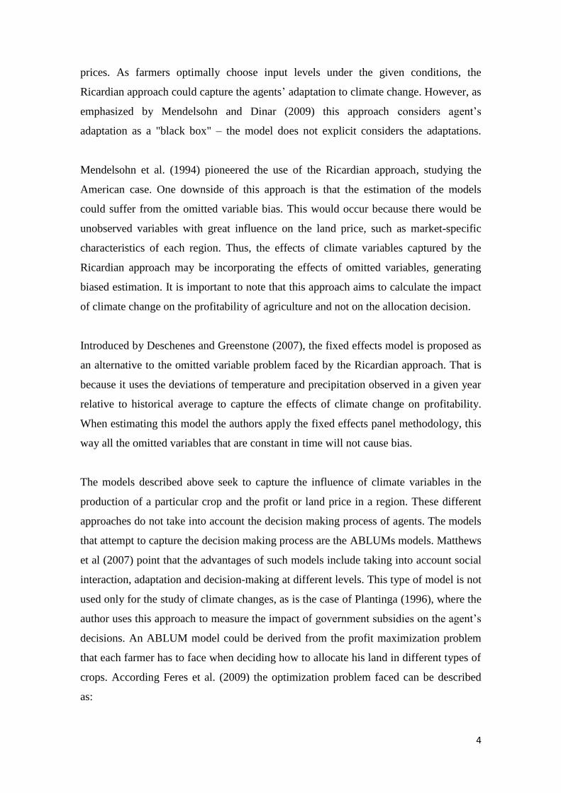
prices. As farmers optimally choose input levels under the given conditions, the

Ricardian approach could capture the agents’ adaptation to climate change. However, as

emphasized by Mendelsohn and Dinar (2009) this approach considers agent’s

adaptation as a "black box" – the model does not explicit considers the adaptations.

Mendelsohn et al. (1994) pioneered the use of the Ricardian approach, studying the

American case. One downside of this approach is that the estimation of the models

could suffer from the omitted variable bias. This would occur because there would be

unobserved variables with great influence on the land price, such as market-specific

characteristics of each region. Thus, the effects of climate variables captured by the

Ricardian approach may be incorporating the effects of omitted variables, generating

biased estimation. It is important to note that this approach aims to calculate the impact

of climate change on the profitability of agriculture and not on the allocation decision.

Introduced by Deschenes and Greenstone (2007), the fixed effects model is proposed as

an alternative to the omitted variable problem faced by the Ricardian approach. That is

because it uses the deviations of temperature and precipitation observed in a given year

relative to historical average to capture the effects of climate change on profitability.

When estimating this model the authors apply the fixed effects panel methodology, this

way all the omitted variables that are constant in time will not cause bias.

The models described above seek to capture the influence of climate variables in the

production of a particular crop and the profit or land price in a region. These different

approaches do not take into account the decision making process of agents. The models

that attempt to capture the decision making process are the ABLUMs models. Matthews

et al (2007) point that the advantages of such models include taking into account social

interaction, adaptation and decision-making at different levels. This type of model is not

used only for the study of climate changes, as is the case of Plantinga (1996), where the

author uses this approach to measure the impact of government subsidies on the agent’s

decisions. An ABLUM model could be derived from the profit maximization problem

that each farmer has to face when deciding how to allocate his land in different types of

crops. According Feres et al. (2009) the optimization problem faced can be described

as:

5

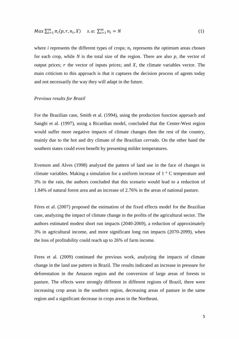
(1)

where i represents the different types of crops; represents the optimum areas chosen

for each crop, while N is the total size of the region. There are also , the vector of

output prices; the vector of inputs prices; and , the climate variables vector. The

main criticism to this approach is that it captures the decision process of agents today

and not necessarily the way they will adapt in the future.

Previous results for Brazil

For the Brazilian case, Smith et al. (1994), using the production function approach and

Sanghi et al. (1997), using a Ricardian model, concluded that the Center-West region

would suffer more negative impacts of climate changes then the rest of the country,

mainly due to the hot and dry climate of the Brazilian cerrado. On the other hand the

southern states could even benefit by presenting milder temperatures.

Evenson and Alves (1998) analyzed the pattern of land use in the face of changes in

climate variables. Making a simulation for a uniform increase of 1 ° C temperature and

3% in the rain, the authors concluded that this scenario would lead to a reduction of

1.84% of natural forest area and an increase of 2.76% in the areas of national pasture.

Féres et al. (2007) proposed the estimation of the fixed effects model for the Brazilian

case, analyzing the impact of climate change in the profits of the agricultural sector. The

authors estimated modest short run impacts (2040-2069), a reduction of approximately

3% in agricultural income, and more significant long run impacts (2070-2099), when

the loss of profitability could reach up to 26% of farm income.

Feres et al. (2009) continued the previous work, analyzing the impacts of climate

change in the land use pattern in Brazil. The results indicated an increase in pressure for

deforestation in the Amazon region and the conversion of large areas of forests to

pasture. The effects were strongly different in different regions of Brazil, there were

increasing crop areas in the southern region, decreasing areas of pasture in the same

region and a significant decrease in crops areas in the Northeast.

6

Although the studies did not present the same results and any comparison between them

should be made with great caution due to the use of different methodologies and

database, the studies show an overall negative effect in the country and different

impacts in different regions of Brazil. The Center-West, North and Northeast appear to

be those which would suffer greater losses due to climate change, while the South could

even benefit from any increase in its average temperature.

3. Methodology

As discussed in the previous section, Féres et. al. (2009) described a model for land use

based on microeconomic theoretical assumptions on the profit-maximizing behavior of

agents. Based on this model, this study presents an innovation, which is the introduction

of specific crops as well as different types of land use. Besides, a more thorough

discussion on the econometric estimation of the coefficients is proposed.

The use of models with aggregated crops in the study of impacts of climate change on

land use can lead to less accurate results, since it is expected that different crops respond

differently to climate changes. Also, analysis of regional impacts of climate changes on

the land use pattern demonstrated that the disaggregation of the different types of crops

provides valuable information to be used in public policy decision-making processes

(e.g. regarding infrastructure investments or mitigation policies). Thus, the following

different types of land use are considered in this study: soybean, corn, sugar cane, other

crops, pasture and forest. Together, the cultivated areas of the three above cited cultures

account for approximately 60% of crops area of Brazil. Hence, a better understanding of

the impacts of climate change on land use for the three referred crops provides relevant

information on the economic impacts of climate change on the Brazilian agricultural

sector.

The presentation of the methodology of the land use model in the present study was

divided into three parts: the economic model, the econometric specification and the

simulation, as shown in the next sub-sections.

3.1. Economic Model

7

The land use model adopted in the present study is the same suggested by Féres et al

(2009). This model is based on the problem of profit maximization by a representative

agent. Given product prices, input costs and the characteristic features of the climate of

each region, the agent must choose the allocation of the different types of land use that

maximizes profit. Or else, the agent allocates land among the different options: soybean,

corn, sugar cane, other crops, pasture and forest in the land in order to maximize profit.

Then we have the following constrained maximization problem:

(2)

where the subscript i indicates the activity performed , is the vector of prices of the

products of agricultural activities, is the vector of prices for inputs, is the area

allocated to activity i, is the vector of agroclimatic variables and is the entire

available land area. There are six types of land use in the developed model, so .

The restriction imposed by the maximization hypothesis simply means that the sum of

the areas allocated to the different activities cannot exceed the entire land area.

The following Lagrangian theorem is used to solve the problem proposed in (2):

(3)

And the following first order conditions arise:

,i = 1, 2, 3, 4, 5 e 6. (4)

(5)

From the above conditions, one can obtain optimal allocations for each type of land use

( ), as a function of the price of the products, input prices, the entire land area and the

agroclimatic variables of the land area. Then, six equations determine the optimum area

for each type of land use:

, for i = soybean, corn, sugar cane, other crops, pasture and forest.

8

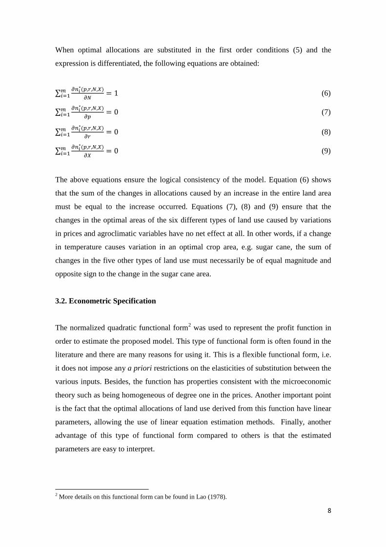
When optimal allocations are substituted in the first order conditions (5) and the

expression is differentiated, the following equations are obtained:

(6)

(7)

(8)

(9)

The above equations ensure the logical consistency of the model. Equation (6) shows

that the sum of the changes in allocations caused by an increase in the entire land area

must be equal to the increase occurred. Equations (7), (8) and (9) ensure that the

changes in the optimal areas of the six different types of land use caused by variations

in prices and agroclimatic variables have no net effect at all. In other words, if a change

in temperature causes variation in an optimal crop area, e.g. sugar cane, the sum of

changes in the five other types of land use must necessarily be of equal magnitude and

opposite sign to the change in the sugar cane area.

3.2. Econometric Specification

The normalized quadratic functional form2 was used to represent the profit function in

order to estimate the proposed model. This type of functional form is often found in the

literature and there are many reasons for using it. This is a flexible functional form, i.e.

it does not impose any a priori restrictions on the elasticities of substitution between the

various inputs. Besides, the function has properties consistent with the microeconomic

theory such as being homogeneous of degree one in the prices. Another important point

is the fact that the optimal allocations of land use derived from this function have linear

parameters, allowing the use of linear equation estimation methods. Finally, another

advantage of this type of functional form compared to others is that the estimated

parameters are easy to interpret.

2 More details on this functional form can be found in Lao (1978).

9

With this function, the following equations that describe optimal allocations of different

land uses to be estimated are obtained:

, i = 1, 2, 3, 4, 5 and 6 (10)

Subject to the following restrictions:

(11)

(12)

(13)

(14)

(15)

Restrictions (11), (12), (13) and (14) are equivalent to those found in equations (6), (7),

(8) and (9). Restriction (15) arises from the symmetry of the normalized quadratic

functional form. Therefore, there is a system of six equations to be estimated, with

observation of the above described restrictions.

According to Matthews et al (2007), agent-based land use models are one way to

incorporate the influence of social interaction, mechanisms of adaptation and decision-

making of agents to the study of land allocation for different uses. In this context, it is

important to understand three different aspects of the problem: the spatial aspect, the

simultaneity of the equations and the temporal dynamics of the problem.

Kumar (2011) argues that the spatial problem must be incorporated into the study of the

impacts of climate changes in agriculture for two reasons: econometric and theoretical.

From a theoretical standpoint, it will be natural to think that the agents distributed

across the space communicate about the activities carried out in each region and

exchange experiences on production practices and techniques that generate a spatial

10

dependence in the dependent variable (crops areas). From an econometric point of view,

a possible inaccuracy in the estimates must be considered due to the presence of spatial

correlation in the error term of the specified equations. Therefore, an estimation method

that considers the spatial factor can lead to improved efficiency of the estimation.

The simultaneous estimation of six equations of optimal allocation of land use is

important because the agents’ decisions occur simultaneously. The allocation of land for

each type of land is made at the same time, and, thus, there is a relationship between the

parameters of the equations. This relationship is described by the restrictions derived

from the economic model, e.g. the parameter that captures the influence of temperature

on a given land use has a relationship with the same parameter in the other equations.

Moreover, the estimation of the system by a non-simultaneous approach does not

consider the possible correlation among residuals.

The temporal dimension should be considered in the study of this problem because, in

order to simulate how agents’ decisions change over time, information on how these

decisions were made at different periods is needed. The aim of this study is to

understand how agents’ decisions are affected by certain variables over time. Hence,

change over time within the same region is a key factor for the correct understanding of

the problem. If only cross-section data over a period of time is considered, we will be

using climatic variations in the different regions to explain the allocation of land use. In

fact, the simulation results tend to show that if the climate pattern in a given region A

becomes similar to the climate pattern in a given region B, then the use of land in region

A would be similar to the use of land in region B.

Thus, in order to estimate the correct way in which the agents of region A adapt to

climate changes it would be necessary to use data from region A at different periods of

time and use temporal variability of climate to explain change in land use. Fixed-effect

panel models would be the most appropriate methodology for this purpose.

Nevertheless, some considerations on the real relationship between climate changes and

land use are necessary in order to define the appropriate methodology for our purposes.

The relationship between historical average temperature and rainfall in each region and

the agricultural activity is clear and direct. Some crops are more productive than others,

11

depending on temperature and rainfall levels, and each region has a comparative

advantage in producing a particular crop. The agent that makes the decision of

allocation seeks to maximize profit and will choose the activities that have a

comparative advantage in the region. The present study is aimed at capturing how

agents would adapt to climate changes in a given region. According to the above

reasoning, we try to understand how the agents in a given region A adapt to changes in

temperature and rainfall in region A. This question can be answered using the variation

in climate data and in land use. However, the key aspect of the decision to use the panel

model would be to check whether already observed climate changes would have

influenced changes in the allocation of land use. Some factors indicate that the answer

to this question is still non-conclusive.

The type of crop grown on a given land tends to be persistent. Several factors must be

taken into consideration when a producer from a region that grows a given crop A

decides to grow another crop B. For this change to occur, besides the greater expected

profit, it takes time for the farmers to learn the different technology related to the new

crop. Also, infrastructure consistent with the new crop is required. Climate variables

could certainly influence this decision, since they would cause one crop to be more

productive than others, and, consequently, would ensure higher profit to the agent.

However, since climate change is a long-term phenomenon, long-term climate data of

the agricultural sector is necessary to capture its impact.

Two issues arise in this type of analysis in the Brazilian case. The first issue is the

reliability of older data for both land use and climate changes, because the older data the

less accurate they are. The second and main issue concerns the central point of our

analysis: the relationship between land use and climate change. Analysis of climate data

already collected shows low temporal variability in temperature and precipitation

variables across the same region. The little temporal variability of climate data and the

persistent decisions on the allocation of land use by agents makes it unlikely that the

change in cultivated areas were related to change in temperature and rainfall. Thus, the

use of the panel model carries a risk of capturing a relationship between climate changes

and land use that does not really exist.

12

For comparison, the equations were estimated using the spatial panel data model

developed by Elhorst (2003), the SAR (Spatial Auto-Regression) with fixed effects. For

this estimation only, data from the agricultural census of 1995 and 2006 were used, and

the temperature and precipitation variables were the averages observed during the last

five years prior to the censuses. The results were not significant for the climate

variables, providing further evidence that climate change over time cannot yet be used

as a justification for the allocation of land use, at least over a not very long period. It

should be noted that several studies used the panel model in the assessment of climate

change impacts on the profitability of the agricultural sector. In this type of study, the

temperature and precipitation data at one moment in time is considered in relation to the

deviation from the historical average, and we can estimate how his deviation influenced

the profitability of the sector.

In view of the question to be answered, and the above discussion, only cross-section

data were estimated. By estimating parameters for cross-sectional data from the 2006

census, only with the purpose of providing a simulation in time, we assume that the

current pattern of land use in Brazil represents the long-run equilibrium between agents,

i.e., agents are making the best possible choices of cultivation areas given the prices and

climate conditions. The simulation based on the estimation of cross-section data has a

long-term character, which is exactly the type of simulation that we intend to make. The

method used was the Iterated Seemingly Unrelated Regression (ISUR) model, the same

used by Feres et al (2009).

Furthermore, in an attempt to capture the spatial factor and at the same time some effect

of temporal inertia, the term W95 was added to the equation, which represents the crop

area in 1995 weighted by the W spatial weight matrix. The matrix used was of the

queen type. The use of a spatially and temporally delayed term is suggested by Lopez

and Chasco (2004) and is aimed to capture the spatial effect throughout time, or else,

the influence of the neighbor does not occur simultaneously, but over time. Hence,

besides capturing the spatial effect of neighbor influence, the term also captures some

temporal inertia in land use in those regions. Another variable included in the model

13

was the crop area in 1996. This term also captures the inertia in land use for different

purposes.3

3.3. Simulation

The simulation of the areas allocated for different uses based on climate forecasts was

made after the estimation of the parameters of the model, according to the following

equation:

(16)

Where is the vector of agroclimatic variables forecasted for the scenario C, and

is the area estimated for land use i, taking into consideration the scenario C. Then, we

can analyze the changes based on the areas observed in the baseline (in this case, the

year of 2006).

Furthermore, when an area allocated to a given crop was negative, the value was

considered 0. In such cases we cannot guarantee that the sum of the new areas allocated

for the different land uses shall be equal to the entire land area in the micro-region.

Then, adjustments are necessary in the simulated to maintain the logical consistency of

the model. Based on the six new areas, the entire new land area was calculated as

follows:

(17)

where represents the entire land area after simulations for region j. We can calculate

the participation of each land use in the simulated region and use this result for

comparison with the total area allocated for each use.

(18)

3 Further discussion on the data used is available in the next section.

14

Finally, the percentage change in the areas allocated for the different land uses is

calculated based on the following expression:

(19)

4. Data

Data from 558 Brazilian microregions were used. The main source of data was the

Brazilian Institute of Geography and Statistics (IBGE), especially the brazilian

agricultural census of 2006. The agronomic data was supplied by Embrapa. The

observed temperature and precipitation were obtained from the Climatic Center Unit

(CRU / University of East Anglia) database and the CPTEC / INPE provided

projections of temperature and precipitation for the period 2010-2099. The construction

of the variables that were used is presented below.

4.1. Land Use

The land use areas were constructed from the information of the agricultural census of

2006. The variable that defines the area for “other crops” corresponds to the sum of

areas of all the permanent and temporary crops other than soybean, sugarcane and corn.

The pasture area is the sum of natural and planted pastures. Finally, the forest area is the

total area of natural forests, planted forests and unused productive land within any

farmer’s establishment.

4.2. Prices of Products: soybeans, corn, sugar cane, crop, pasture and forest

The prices of soybean, corn and sugarcane were calculated based on average values of

tons produced in each microregion. The “other crops” price was constructed as a

Laspeyres index, where the national average was the base value. The index is composed

by the prices and production of the major crops in terms of areas except soybean, corn

and sugarcane: rice, beans, tobacco, cassava, wheat, cotton, bananas, cocoa , coffee and

orange. The representative price of the products of the pasture activity was the average

price of cattle sold in the microregion. The price of the products of forests was

15

represented by the average per cubic (m3) value of timber in the microregion. The

hypothesis is that the price of timber is a good proxy for the opportunity cost of

conserving forest areas in agricultural establishments.

Except for the price of cattle, which was observed in the agricultural census of 2006, all

other prices were the average price of the five years preceding the census data (the cattle

price was the not available for the period in the microregional level). The choice of

using this prices instead of the prices observed in the census is related to the decision-

making of the agents. The future relative prices that guide the agent’s decision are

formed based on the recent prices that the agents observed. All prices used in the model

correspond to 2006 values.

4.3. Prices of Inputs: land and labor

In this study we considered only two inputs for agricultural production: land and labor.

There is no regional data for land prices in Brazil so the land leasing price was used as a

proxy. The labor price was represented by the average rural wage, given by the total

monetary value of wages (in cash or goods) paid to employees or family members

divided by the total number of persons employed.

4.4. Observed Climate variables

Variables for temperature (°C) and precipitation (mm) were used in the model. The

information was consolidated from the CRU / University of East Anglia data base and

represent a 30 years average of the data from 1975 to 2005. For each season (3 months

period) a different variable for temperature and precipitation was constructed. This is

important because the effects of climate change in agriculture can be different

depending on the season.

4.5. Projected Climate variables

The temperature and precipitation projections for Brazil in the period of 2010-2099,

were obtained from the CPTEC / INPE. The PRECIS (Providing Regional Climates for

Impact Studies) model provides projections for two emission scenarios defined by IPCC

16

(International Panel on Climate Change), A2 and B2, and both were considered in the

simulations.

The PRECIS model provides monthly forecasts of climate variables; however, in the

present study 30 years averages were calculated for the following years: 2010-2039,

2040-2069 and 2070-2099. Working with averages of precipitation and temperature are

adequate for two main reasons. First, it is reasonable to expect that the land allocation

decisions take into account the behavior of the climate variables especially in the long

run. Furthermore, when calculating the average over this relatively long period, we

reduce the "uncertainty" inherent in climate projection models. The downside of

working with these averages is the fact that the effects of extreme events would be

diluted into the average and will not be captured by the model.

5. Results

In this section the econometrics results of the model’s estimation are presented followed

by the simulations results.

5.1. Land Use Model

As discussed in section 4, the estimation of the optimal land allocations equations was

made by the ISUR methodology. The model was estimated for the 6 types of land uses

according to equation 10. Furthermore, the model was estimated considering all the

mentioned parametric restrictions. Table 1 presents the results of the estimation.

17

Table 1. Regression Results

The temperature and precipitation variables were significant in almost all equations. In

the sugarcane and other crops equations some variables of temperature and precipitation

were not significant. This is evidence that temperature and precipitation are determinant

factors in the land use allocation by farmers. It is also interesting to note the signal

differences found when comparing the climatic variables for different seasons, this

occurs in all the equations, justifying the use of season averages instead of the annual

averages of the variables. Both for temperature and for the precipitation in summer and

winter an increase in the magnitude of these variables favors the increase of the pasture

area and the decrease in the cultivated area of all other uses. As for the spring and

Equation

Coef. t-stat p-value Coef. t-stat p-value Coef. t-stat p-value

Relative Price Soybean 75507.32 1.91 0.06 25356.08 1.79 0.07 8283.37 2.28 0.02

Relative Price Corn -96696.39 -1.79 0.07 -36474.01 -1.90 0.06 -8209.29 -1.66 0.10

Relative Price Sugarcane 37809.36 0.76 0.45 13757.95 0.79 0.43 -8415.60 -1.59 0.11

Relative Price Other Crops -2.22 -2.17 0.03 -0.47 -1.28 0.20 -0.06 -0.70 0.49

Relative Price Forest -22900.91 -0.54 0.59 1414.88 0.09 0.93 -2252.55 -0.42 0.67

Relative Price Land 211.67 0.07 0.95 83.17 0.08 0.94 -72.58 -0.26 0.80

Relative Price Labor 1631.84 1.92 0.05 612.37 2.11 0.04 101.21 1.27 0.20

Temperature DJF -69747.35 -3.06 0.00 -17829.04 -2.28 0.02 -1477.25 -0.71 0.48

Temperature MAM 100732.60 3.67 0.00 22259.71 2.36 0.02 3507.05 1.39 0.16

Temperature JJA -65328.65 -3.17 0.00 -19217.82 -2.72 0.01 -3066.49 -1.62 0.11

Temperature SON 39707.11 2.12 0.03 16317.79 2.54 0.01 2118.43 1.23 0.22

Precipitation DJF -2101.58 -6.47 0.00 -912.46 -8.18 0.00 -45.45 -1.52 0.13

Precipitation MAM 2475.95 7.39 0.00 953.93 8.26 0.00 59.49 1.93 0.05

Precipitation JJA -1082.50 -3.35 0.00 -491.13 -4.43 0.00 -15.08 -0.50 0.62

Precipitation SON 1760.40 5.07 0.00 645.30 5.41 0.00 26.09 0.82 0.41

AreaTot 0.05 8.17 0.00 0.02 7.54 0.00 0.00 -0.43 0.66

W95 0.10 3.32 0.00 -0.30 -5.13 0.00 0.14 3.12 0.00

_cons -283682.70 -1.45 0.15 -44369.70 -0.65 0.51 -35676.97 -1.97 0.05

Rsq = 0.4422 Rsq = 0.5800 Rsq = 0.8439

SOYBEAN CORN SUGARCANE

Equation

Coef. t-stat p-value Coef. t-stat p-value Coef. t-stat p-value

Relative Price Soybean 9894.47 0.68 0.50 -146881.60 -1.92 0.06 21558.51 0.37 0.71

Relative Price Corn -16909.80 -0.85 0.40 140240.40 1.32 0.19 22104.52 0.28 0.78

Relative Price Sugarcane 40212.66 2.19 0.03 -97188.51 -1.02 0.31 3231.00 0.04 0.97

Relative Price Other Crops -0.19 -0.51 0.61 4.05 2.13 0.03 -0.96 -0.67 0.51

Relative Price Forest -33198.00 -2.09 0.04 103830.60 1.28 0.20 -30751.86 -0.50 0.62

Relative Price Land -268.26 -0.24 0.81 641.98 0.11 0.92 -595.98 -0.13 0.90

Relative Price Labor -1020.26 -3.31 0.00 1733.55 1.02 0.31 -3058.70 -2.39 0.02

Temperature DJF -31752.74 -3.80 0.00 324819.10 7.16 0.00 -204012.70 -5.94 0.00

Temperature MAM 35987.36 3.59 0.00 -288271.10 -5.25 0.00 125784.40 3.03 0.00

Temperature JJA -14920.47 -1.99 0.05 165937.90 4.03 0.00 -63404.51 -2.04 0.04

Temperature SON 4685.87 0.69 0.49 -150590.50 -4.03 0.00 87761.32 3.11 0.00

Precipitation DJF -133.71 -1.12 0.26 4859.89 7.51 0.00 -1666.68 -3.41 0.00

Precipitation MAM 176.81 1.44 0.15 -5798.79 -8.70 0.00 2132.62 4.23 0.00

Precipitation JJA -81.37 -0.69 0.49 3178.13 4.93 0.00 -1508.05 -3.09 0.00

Precipitation SON 64.61 0.51 0.61 -4586.99 -6.63 0.00 2090.60 4.00 0.00

AreaTot 0.00 1.53 0.13 0.62 52.74 0.00 0.31 34.60 0.00

W95 0.05 1.70 0.09 0.02 4.24 0.00 -0.01 -1.10 0.27

_cons 171399.00 2.34 0.02 -984571.10 -2.52 0.01 1150425.00 3.90 0.00

Rsq = 0.5007 Rsq = 0.9068 Rsq = 0.8376

OTHER CROPS PASTURE FOREST

18

autumn, the effect is the opposite. The climate variables seem to affect the pasture use

in an opposite way then they affect the other land uses.

One point of attention in the estimation of the model is the coefficients of the relative

price variables. Most of these coefficients are not statistically significant, and the sign of

the coefficient is not consistent with that expected by economic theory. For example,

the coefficient for the corn price shows that an increase of the corn price would reduce

the area for this crop. The way the price variables were constructed (from the average in

the years preceding the census) should reflect the expectation of prices in each region

and therefore be an important factor in the decision to land use. However, the model

cannot adequately capture the effect of the price of crops in the land allocation decision.

One possible explanation for this is the low volume of production of some crops in

certain regions, which may cause distortions in relative prices. There could be also a

problem of endogeneity on the price variables and subsequently an identification

problem. The area designated for the production of a certain crop could influence the

price of this crop product. The construction of the price variables is certainly a

challenge and a point of improvement for future works.

Finally, the variable W95 was significant in all equations, except on those for forest and

other crops. This demonstrates the importance of the spatial lag on the model. In this

case, the neighbor’s allocation decision in the previous period has an influence on land

use of a region in the current period. In the equations for soybean, sugarcane, other

crops and pasture, the coefficients were found to be positive. We observe a positive

influence of the neighbors land use in the previous period in the land allocation

decisions in 2006. This indicates a consolidation of this type of land use in the regions.

As for corn and forests the coefficients were negative, indicating that there was no

consolidation of these crops in the regions.

5.2. Simulations

One should be careful in analyzing the simulation results; it is important to understand

that the simulations should be interpreted as responses to the following conjecture:

given the technological and productive structures for 2006 and the climate variables

changes projected by the CPTEC / INPE, how would the optimal allocations of land

19

behave once the total area occupied by each of the farms remains the same? The

simulations do not capture possible changes in other variables that determine land use,

such as product prices. It is natural to think that if the area of a given crop had a

significant reduction, and consequently there were a decrease in the supply of its

product, its price would likely increase, providing incentive for further production of it.

Thus, the simulations made here tend to overestimate the variations in the areas, since

we are not capturing the second-order effects of price changes. It is also natural to think

that an increase in the acreage of a particular crop would lead to an increase in the

domestic production, and, therefore, to a potential decrease in prices, which in turn

would induce a reduction in cultivated area.

5.2.1. Simulations – National results

Table 2 presents the simulation results for Brazil as a whole, both in percentage and in

ordinary (hectares) changes.

Table 2. Simulation Results - Percentage and Thousand Hectares variation

In both scenarios (A2 and B2), pastures lands, which already accounted for the largest

share of the establishments’ areas, would gain even more participation over the years.

When analyzing the absolute numbers of the pasture areas it can be noted that the

increase would be mainly due to forests areas reductions on farms. Although the

Period Soybean Corn Sugarcane O. Crops Pasture Forest

83% 30% -9% -38% 16% -31%

12983.1 3733.1 -529.9 -10538.6 26449.2 -32096.9

78% 27% -7% -44% 24% -42%

12173.9 3410.7 -424.8 -12125.6 40369.8 -43403.9

81% 31% -8% -55% 35% -58%

12631.2 3836.6 -485.9 -15350.0 58845.6 -59477.5

Soybean Corn Sugarcane O. Crops Pasture Forest

81% 27% -10% -38% 18% -33%

12618.7 3374.7 -599.3 -10607.7 29325.7 -34112.2

80% 27% -8% -42% 20% -36%

12558.6 3406.0 -466.0 -11567.1 33101.3 -37032.7

84% 29% -8% -45% 24% -43%

13189.9 3632.3 -439.6 -12476.6 40666.2 -44572.2

2039

2069

2099

A2

B2

2039

2069

2099

20

reduction of forest areas and the increase of pasture areas are observed in both

scenarios, it is interesting to note that the magnitude of these changes are greater in the

A2 scenario. Forest areas would suffer a reduction of 58% and 43% respectively for the

A2 and B2 scenarios. While there would be an increase of 35% and 24% respectively in

pastures for the scenarios A2 and B2.

There would be also a sharp drop in the participation of other crops, initially similar in

both scenarios, but also of greater magnitude in the A2 scenario when the time horizon

is greater. The model indicates a potential decrease of almost 40% of the area for this

type of use already in the years 2010 to 2039 in both scenarios.

There would be a distinct pattern for sugarcane compared to soybeans and corn. The

simulations show a decrease in sugarcane areas and an increased on soybean and corn

areas.

Table 3 shows the change in the pattern of land use observed in the simulations,

depicting how the land use structure could be affected.

Table 3. Land Use Share

5.2.2. Simulations – Regional results

It is also important to analyze the results in a regional perspective. Tables 4 to 8 present

the results for each of the 5 Brazilian regions. The regional highlights are the following:

Decrease of more then 50% on forests areas in the north region and a subsequent

increase in pasture areas.


2006 4.7% 3.8% 1.8% 8.4% 50.3% 31.1%

2010-39 8.6% 4.9% 1.6% 5.2% 58.3% 21.4%

2040-60 8.4% 4.8% 1.6% 4.7% 62.5% 18.0%

2070-99 8.5% 4.9% 1.6% 3.8% 68.0% 13.2%

2010-39 8.5% 4.8% 1.6% 5.2% 59.1% 20.8%

2040-60 8.5% 4.8% 1.6% 4.9% 60.3% 19.9%

2070-99 8.7% 4.9% 1.6% 4.6% 62.6% 17.7%

A2

B2

Brazil

21

Decrease in sugar cane and forest areas in the northeast region and an increase in

pasture areas.

Decrease of more than 70% of the forests in the southeast region. Also a

considerable increase in the corn and soybean areas for this region.

Decrease of pasture lands in the south, and an increase in soybean, corn and

sugarcane areas. There is also a potential increase on the forests areas in the

medium run and.

A decrease in the forest areas and an increase in the soybean, corn and sugarcane

areas for the center-west region.

Table 4. North Region – Simulation Results – Percentage and Thousand Hectares

Variation


262% 156% 290% -39% 36% -42%

589.2 461.0 61.9 -1446.4 9869.3 -9535.0

235% 129% 397% -45% 44% -51%

527.3 382.2 84.8 -1647.7 12203.1 -11549.7

227% 160% 611% -56% 57% -65%

509.8 471.6 130.4 -2036.0 15771.2 -14846.9


283% 150% 304% -38% 36% -43%

635.5 444.0 64.9 -1404.6 9979.0 -9718.8

252% 139% 360% -42% 38% -44%

566.0 411.1 76.9 -1533.7 10516.7 -10037.0

200% 114% 429% -47% 46% -52%

450.2 337.3 91.6 -1734.4 12807.8 -11952.5

2069

2099

2099

B2

2039

A2

2039

2069

22

Table 5. Northeast Region – Simulation Results – Percentage and Thousand

Hectares Variation

Figure 6. Southeast Region – Simulation Results – Percentage and Thousand

Hectares Variation


13% -63% -59% -55% 60% -51%

144.1 -2125.6 -678.0 -5475.9 21068.5 -12933.2

18% -61% -57% -59% 66% -59%

196.8 -2044.3 -654.1 -5801.6 23267.2 -14964.0

35% -56% -52% -63% 75% -71%

388.1 -1892.3 -597.6 -6223.0 26387.2 -18062.4


-1% -65% -60% -56% 62% -53%

-10.4 -2198.1 -679.0 -5537.2 21943.3 -13518.5

-10% -66% -59% -59% 65% -56%

-107.4 -2210.3 -678.0 -5804.9 22942.1 -14141.4

65% -49% -53% -57% 62% -58%

724.7 -1655.2 -609.6 -5654.0 21810.3 -14616.32099

B2

2039

2069

A2

2039

2069

2099


346% 61% -9% -36% 20% -59%

3244.6 1209.7 -339.2 -2465.3 5800.0 -7449.8

319% 50% -10% -43% 31% -75%

2991.8 990.5 -366.0 -2966.4 8723.1 -9373.1

278% 35% -18% -60% 44% -88%

2600.0 685.2 -652.2 -4088.0 12461.2 -11006.3


320% 50% -12% -38% 26% -67%

2996.7 983.0 -418.8 -2609.9 7456.6 -8407.5

306% 48% -10% -42% 28% -69%

2864.7 949.0 -366.6 -2847.9 8016.8 -8616.1

292% 35% -14% -48% 35% -78%

2738.9 701.0 -490.0 -3257.5 10082.1 -9774.4

2069

2099

B2

2039

2069

2099

A2

2039

23

Table 7. South Region – Simulation Results – Percentage and Thousand Hectares

Variation

Table 8. Center-West Region – Simulation Results – Percentage and Thousand

Hectares Variation


69% 45% 73% -10% -58% 27%

4667.0 1997.4 295.4 -429.9 -9272.6 2742.8

70% 48% 89% -15% -41% 1%

4755.5 2114.3 363.4 -649.8 -6653.7 70.3

81% 57% 108% -34% -17% -42%

5501.4 2528.5 439.5 -1462.0 -2694.7 -4312.7


69% 45% 75% -8% -57% 24%

4682.7 1982.3 305.8 -345.1 -9137.2 2511.4

72% 47% 86% -12% -52% 15%

4910.9 2086.6 351.2 -521.2 -8390.8 1563.3

79% 51% 99% -17% -43% -3%

5408.2 2268.4 402.1 -738.6 -7005.4 -334.8

A2

2039

2069

2099

B2

2039

2069

2099


66% 90% 21% -23% -2% -15%

4338.2 2190.6 130.0 -721.0 -1016.1 -4921.7

56% 81% 23% -35% 5% -24%

3702.4 1967.9 147.1 -1060.1 2830.0 -7587.4

55% 84% 31% -50% 12% -35%

3631.9 2043.7 194.0 -1541.0 6920.7 -11249.1


66% 89% 20% -23% -2% -15%

4314.3 2163.6 127.8 -710.9 -915.9 -4978.9

66% 89% 24% -28% 0% -18%

4324.4 2169.6 150.5 -859.4 16.5 -5801.6

59% 81% 26% -36% 5% -24%

3867.9 1980.9 166.2 -1092.0 2971.2 -7894.2

A2

2039

2069

2099

B2

2039

2069

2099

24

6. Final Remarks

The present study aimed to assess the expected impact of climate change on the land use

patterns in Brazil. An econometric model was estimated in order to understand the

climate impacts on the land allocation decision by farmers for six possible uses:

soybeans, corn, sugarcane, other crops, pastures and forests. Simulations of the optimal

land allocations for the years between 2010 and 2099 were conducted based on

temperature and precipitation projections.

The coefficients used on the simulations were estimated from the system of equations,

derived from the economic model, by a simultaneous equations estimation method

(ISUR). This method was chosen based on the discussion on the best way to capture the

climatic changes impacts on land use. Although the literature shows numerous

applications using panel data for estimating climate change impacts on the agriculture

sector, the discussions carried out in this chapter supported the use of the cross-section

estimation to solve the proposed problem.

The simulation results suggest, at the national level, a significant expansion of the

pasture area at the expense of other land uses. In particular areas of “other crops” and

forests would be negatively affected. It is noteworthy that the results point to greater

changes than those found by Féres et al. (2009), although both studies point to an

increase in pasture areas and decrease in forest areas. The simulations suggested that,

given the expected spatial heterogeneity of climate change, the effects can be quite

different depending on the region.

Although the results point to percentage changes of great magnitude, when analyzing

the effects of the impacts on the share of each of the six land uses presented in the study

we observe that the structural change is not so significant. Pastures, which currently

have the greater share of the land use, would remain with the largest participation in all

regions.

After performing the simulations it is important to note the limitations of the

projections. The first one was the low significance of the price variables, which were

not statistically significant in many cases, and also presented in some cases a different

25

sign than the expected by economic theory. The results would not be capturing correctly

the expected influence of relative prices in the land use decision. Another limiting factor

in the analysis performed in this study is the overestimation of the impacts. This is so

due to the fact that the simulations do not take into account the second-order effects of

re-allocation of land use. For example, the decrease in the cultivation area of sugarcane

could probably increase the price of the product, and consequently generate a greater

incentive to the sugarcane cultivation.

Despite the limitations, the results provide important insights on the likely impacts of

climate change on the Brazilian land use patterns, showing potential decreases in forest

areas in favor of pasture fields.

References

Adams, R. (1989). Global climate change and agriculture: an economic perspective.

American Journal of Agricultural Economics, December, 71(5), pp. 1272-79.

Chasco, C. & López, F.A., 2004. "Modelos de regresión espacio-temporales en la

estimación de la renta municipal: el caso de la Región de Murcia," Estudios de

Economía Aplicada, Estudios de Economía Aplicada, vol. 22, pages 1-24, Diciembre

Dale, V.H. (1997) The Relationship Between land-use change and climate change.

Ecological Applications 7:3, 753-769

Decker, W.L., V. Jones, and R. Achtuni. (1986). The Impact of Climate Change from

Increased Atmospheric Carbon Dioxide on American Agriculture. DOE/NBB-0077.

Washington, DC: U.S. Department of Energy.

Dêschenes, Olivier and Michael Greenstone (2007). “The Economic Impacts of Climate

Change: Evidence from Agricultural Output and Random Fluctuations in Weather”.

American Economic Review, 97(1): 354-85.

Elhorst, J. P. (2003) Specification and estimation of spatial panel data models. Int Reg

Sci Rev 26(3):244-268

Evenson, R.E. & D.C.O. Alves (1998). Technology, climate change, productivity and

land use in Brazilian agriculture. Planejamento e Políticas Públicas, 18, pp.223-258.

Féres, J., E. Reis e J. Speranza. Mudanças climática globais e seus impactos sobre os

padrões de uso do solo no Brasil. In: XXXVII Encontro Nacional de Economia,

2009, Foz do Iguaçu. Anais do XXXVII Encontro Nacional de Economia, 2009.

Disponível em: http://www.anpec.org.br/encontro_2009.htm

http://ideas.repec.org/a/lrk/eeaart/22_3_10.html

http://ideas.repec.org/a/lrk/eeaart/22_3_10.html

http://ideas.repec.org/s/lrk/eeaart.html

http://ideas.repec.org/s/lrk/eeaart.html

26

Féres, J., E. Reis e J. Speranza (2007). Assessing the Impact of Climate Change on the

Brazilian Agricultural Sector. In: Proceedings of the 16th

Annual EAERE Annual

Conference. Gothemburg: European Association of Environmental and Resource

Economists.

Kumar K.S. (2011) “Climate sensitivity of Indian agriculture: do spatial effects

matter?” Cambridge Journal of Regions, Economy and Society 2011, 1-15

Lau, L. J. “Applications of Profit Functions.” Production Economics: A Dual Approach

to Theory and Applications, Vol. 1, eds., M. Fuss and D. McFadden, Cap. I.3.

Amsterdam: North-Holland, 1978.

Mendelsohn, R., W. Nordhaus, e D. Shaw (1994). The Impact of Global Warming on

Agriculture: A Ricardian Analysis. American Economic Review. 84(4): 753-71

Mendelsohn, Robert, William D. Nordhaus and Daigee Shaw (1999). “The Impact of

Climate Variation on US Agriculture”. In The Impact of Climate Change on the

United States Economy, ed. Robert Mendelsohn and James E. Neumann, 55-74.

Cambridge: Cambridge University Press.

Matthews, RB, Gilbert, NG, Roach, A, Polhill, JG and Gotts, NM (2007) Agent-based

land-use models: a review of applications Landscape Ecology, 22 (10). 1447 – 1459

Moore, M.R., e Negri, D.H. “A Multicrop Production Model of Irrigated Agriculture,

Applied to Water Allocation Policy of the Bureau of Reclamation” J. Agr. and Res.

Econ. 17:29-43.

Platinga, A. J. (1996) “The Effect of Agricultural Policies on Land Use and

Environmental” American Journal of Agricultural Economics, Vol. 78, No. 4 (Nov.,

1996), pp. 1082-1091

Sands, R.D. and J.A. Edmonds (2005), “Climate change impacts for the conterminous

USA: an integrated assessment – Part 7. Economic analysis of field crops and land

use with climate change”, Climate Change, 69, 127-50

Sanghi, A., D. Alves, R. Evenson, and R. Mendelsohn (1997). Global warming impacts

on Brazilian agriculture: estimates of the Ricardian model. Economia Aplicada,

v.1,n.1,1997.

Siqueira, O.J.F. de, J.R.B. de Farias, and L.M.A. Sans (1994). Potential effects of

global climate change for Brazilian agriculture, and adaptive strategies for wheat,

maize, and soybeans. Revista Brasileira de Agrometeorologia, Santa Maria, v.2 pp.

115-129.

Documents

CLIMATE CHANGE AND LAND USE PATTERN IN BRAZIL