Classification - Department of Computer and Information Science

University of Florida CISE department Gator Engineering

Classification Part 1

Dr. Sanjay Ranka Professor

Computer and Information Science and Engineering University of Florida, Gainesville


Data Mining Sanjay Ranka Spring 2011

Overview • Introduction to classification • Different techniques for classification • Decision Tree Classifiers

– How decision tree works? – How to build a decision tree? – Methods for splitting – Measures for selecting the best split – Practical Challenges in Classification – Handling over-fitting – Handling missing attribute values – Other issues



Classification : Definition • Given a set of records (called the training set)

– Each record contains a set of attributes – One of the attributes is the class

• Find a model for the class attribute as a function of the values of other attributes

• Goal: Previously unseen records should be assigned to a class as accurately as possible – Usually, the given data set is divided into training

and test set, with training set used to build the model and test set used to validate it. The accuracy of the model is determined on the test set.



• In general a classification model can be used for the following purposes: – It can serve as a explanatory tool for

distinguishing objects of different classes. This is the descriptive element of the classification model

– It can be used to predict the class labels of new records. This is the predictive element of the classification model

Classification Model



General Approach • To build a classification model, the labeled

data set is initially partitioned in to two disjoint sets, known as training set and test set, respectively

• Next, a classification technique is applied to the training set to induce a classification model

• Each classification technique applies a learning algorithm



General Approach • The goal of a learning algorithm is to build

a model that has good generalization capability – That is it must not only fit the training set well

but can also predict correctly the class labels of many previously unseen records

• To evaluate how well the induced model performs on records it has not seen earlier, we can apply it to the test set



General Approach

Test Set

Training Set

Model Learn

Classifier



Classification Techniques • Decision Tree based Methods • Rule-based Methods • Memory based reasoning • Neural Networks • Genetic Algorithms • Naïve Bayes and Bayesian Belief Networks • Support Vector Machines



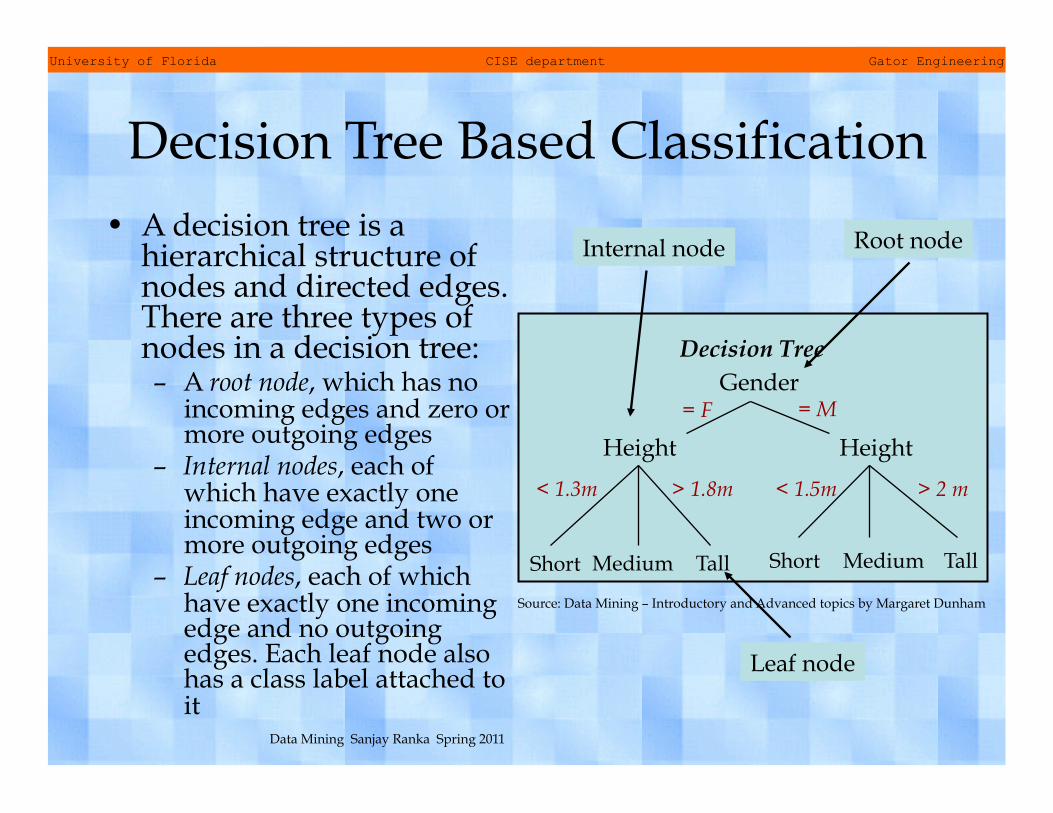
Decision Tree Based Classification • A decision tree is a

hierarchical structure of nodes and directed edges. There are three types of nodes in a decision tree: – A root node, which has no

incoming edges and zero or more outgoing edges

– Internal nodes, each of which have exactly one incoming edge and two or more outgoing edges

– Leaf nodes, each of which have exactly one incoming edge and no outgoing edges. Each leaf node also has a class label attached to it

Decision Tree Gender

Height Height

Medium Tall Medium Tall Short

= F = M

< 1.3m > 1.8m < 1.5m > 2 m

Source: Data Mining – Introductory and Advanced topics by Margaret Dunham

Root node Internal node

Short

Leaf node



Decision Tree Based Classification • One of the most widely used classification

technique • Highly expressive in terms of capturing

relationships among discrete variables • Relatively inexpensive to construct and

extremely fast at classifying new records • Easy to interpret • Can effectively handle both missing values and

noisy data • Comparable or better accuracy than other

techniques in many applications



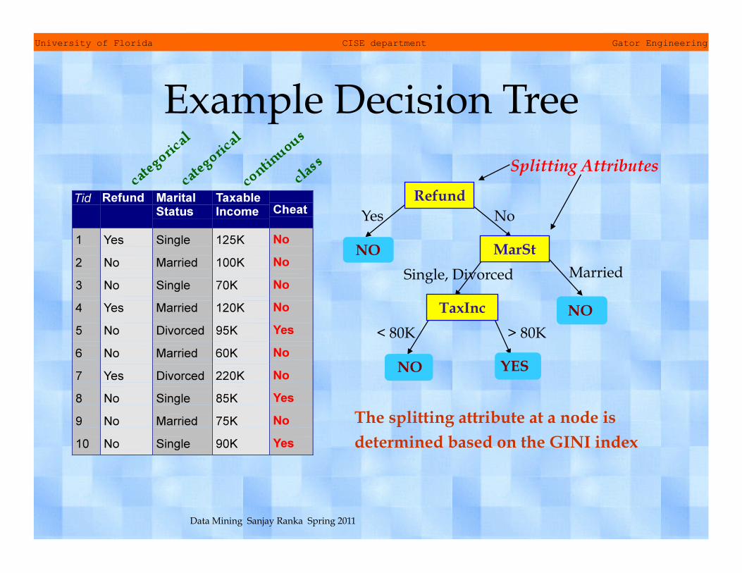
Example Decision Tree

Refund

MarSt

TaxInc

YES NO

NO

NO

Yes No

Married Single, Divorced

< 80K > 80K

Splitting Attributes

The splitting attribute at a node is determined based on the GINI index



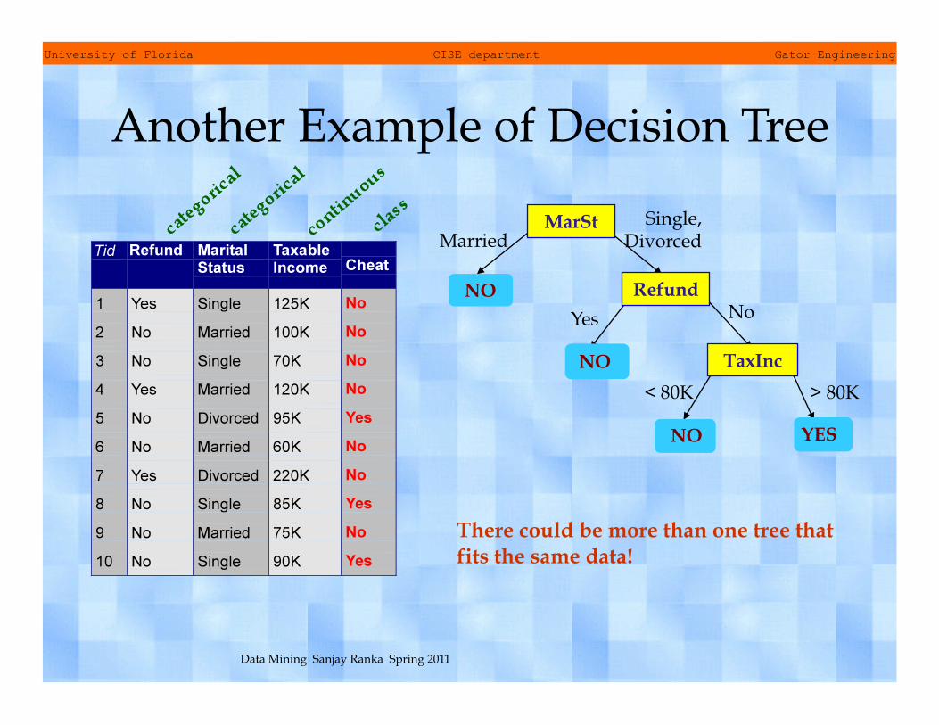
Another Example of Decision Tree

MarSt

Refund

TaxInc

YES NO

NO

NO

Yes No

Married Single,

Divorced

< 80K > 80K

There could be more than one tree that fits the same data!



Decision Tree Algorithms • Many algorithms

– Hunt’s algorithm (one of the earliest) – CART – ID3, C4.5 – SLIQ, SPRINT

• General Structure – Tree induction – Tree pruning



Hunt’s Algorithm • Most of the decision tree induction algorithms

are based on original ideas proposed in Hunt’s Algorithm

• Let Dt be the training set and y be the set of class labels {y1, y2, … , yc} – If Dt contains records that belong to the same class, yk,

then its decision tree consists of leaf node labeled as yk – If Dt is an empty set, then its decision tree is a leaf

node whose class label is determined from other information such as the majority class of the records



Hunt’s Algorithm – If Dt contains records that belong to several

classes, then a test condition, based on one of the attributes of Dt, is applied to split the data in to more homogenous subsets

• The test condition is associated with the root node of the decision tree for Dt. Dt is then partitioned into smaller subsets, with one subset for each outcome of the test condition. The outcomes are indicated by the outgoing links from the root node. This method is then recursively applied to each subset created by the test condition



Example of Hunt’s Algorithm • Attributes: Refund (Yes, No), Marital Status (Single,

Divorced, Married), Taxable Income (continuous) • Class: Cheat, Don’t Cheat

Don’t Cheat

Refund

Don’t Cheat

Don’t Cheat

Yes No Refund

Don’t Cheat

Yes No Marital Status

Don’t Cheat Cheat

Single, Divorced Married

Refund

Don’t Cheat

Yes No Marital Status

Don’t Cheat

Cheat

Single, Divorced Married

Taxable Income

Don’t Cheat

< 80K >= 80K



Tree Induction • Determine how to split the records

– Use greedy heuristics to make a series of locally optimum decision about which attribute to use for partitioning the data

– At each step of the greedy algorithm, a test condition is applied to split the data in to subsets with a more homogenous class distribution

• How to specify test condition for each attribute • How to determine the best split

• Determine when to stop splitting – A stopping condition is needed to terminate tree

growing process. Stop expanding a node • if all the instances belong to the same class • if all the instances have similar attribute values



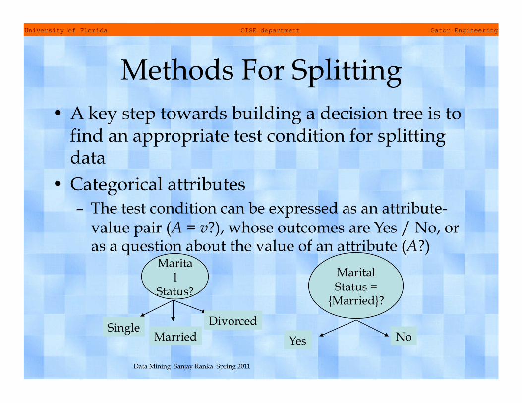
Methods For Splitting • A key step towards building a decision tree is to

find an appropriate test condition for splitting data

• Categorical attributes – The test condition can be expressed as an attribute-

value pair (A = v?), whose outcomes are Yes / No, or as a question about the value of an attribute (A?)

Marital

Status?

Marital Status =

{Married}?

Single Married

Divorced

Yes No



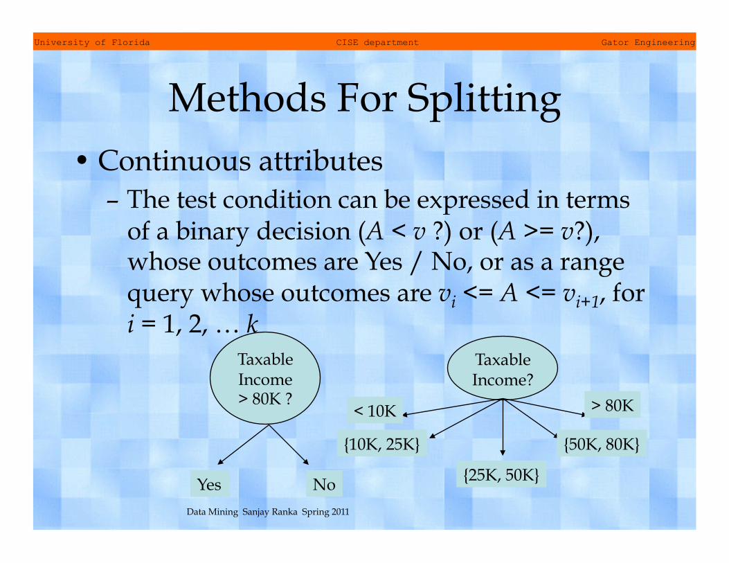
Methods For Splitting • Continuous attributes

– The test condition can be expressed in terms of a binary decision (A < v ?) or (A >= v?), whose outcomes are Yes / No, or as a range query whose outcomes are vi <= A <= vi+1, for i = 1, 2, … k

Taxable Income > 80K ?

Taxable Income?

Yes No

< 10K > 80K

{25K, 50K}

{10K, 25K} {50K, 80K}



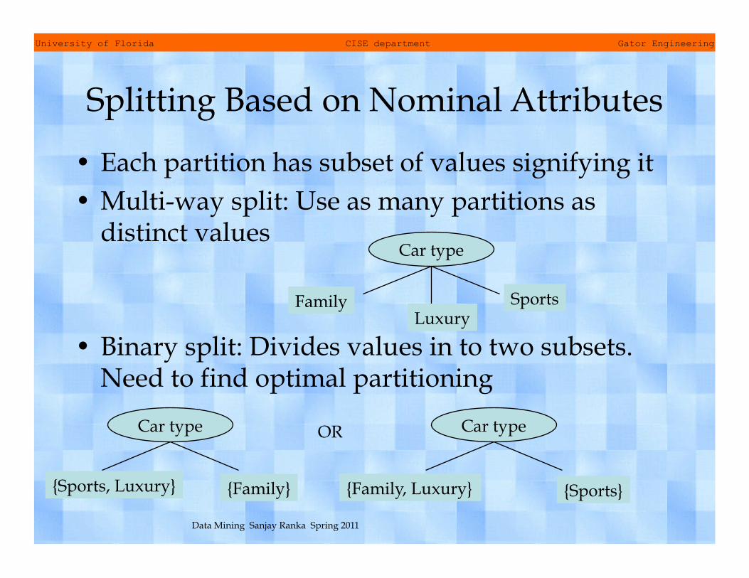
Splitting Based on Nominal Attributes

• Each partition has subset of values signifying it • Multi-way split: Use as many partitions as

distinct values

• Binary split: Divides values in to two subsets. Need to find optimal partitioning

Car type

Family Luxury

Sports

Car type Car type

{Sports, Luxury} {Family} {Family, Luxury} {Sports}

OR



Splitting Based on Ordinal Attributes

• Each partition has subset of values signifying it • Multi-way split: Use as many partitions as distinct

values

• Binary split: Divide values in to two subsets. Need to find optimal partitioning

• What about this split?

Size

Small Medium

Large

Car type

{Small, Medium} {Large}

Car type

{Small} {Medium, Large}

OR

Car type

{Small, Large} {Medium}



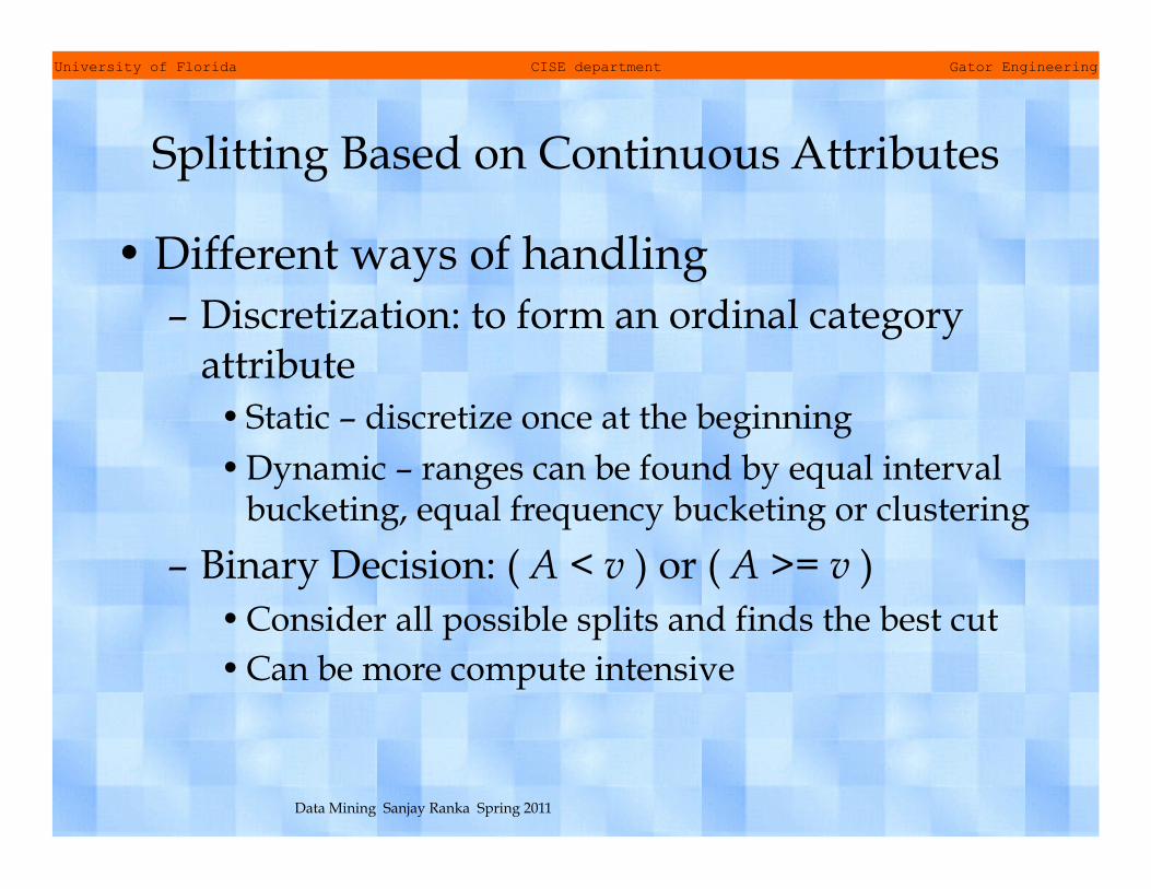
Splitting Based on Continuous Attributes

• Different ways of handling – Discretization: to form an ordinal category

attribute • Static – discretize once at the beginning • Dynamic – ranges can be found by equal interval

bucketing, equal frequency bucketing or clustering

– Binary Decision: ( A < v ) or ( A >= v ) • Consider all possible splits and finds the best cut • Can be more compute intensive



Splitting Criterion • There are many test conditions one could

apply to partition a collection of records in to smaller subsets

• Various measures are available to determine which test condition provides the best split – Gini Index – Entropy / Information Gain – Classification Error



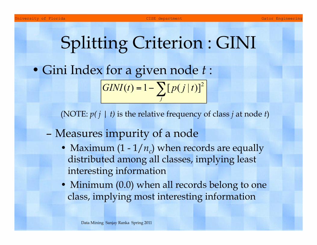
Splitting Criterion : GINI • Gini Index for a given node t :

(NOTE: p( j | t) is the relative frequency of class j at node t)

– Measures impurity of a node • Maximum (1 - 1/nc) when records are equally

distributed among all classes, implying least interesting information

• Minimum (0.0) when all records belong to one class, implying most interesting information



Examples of Computing GINI

p(C1) = 0/6 = 0 p(C2) = 6/6 = 1

Gini = 1 – p(C1)2 – p(C2)2 = 1 – 0 – 1 = 0

p(C1) = 1/6 p(C2) = 5/6

Gini = 1 – (1/6)2 – (5/6)2 = 0.278

p(C1) = 2/6 p(C2) = 4/6

Gini = 1 – (2/6)2 – (4/6)2 = 0.444



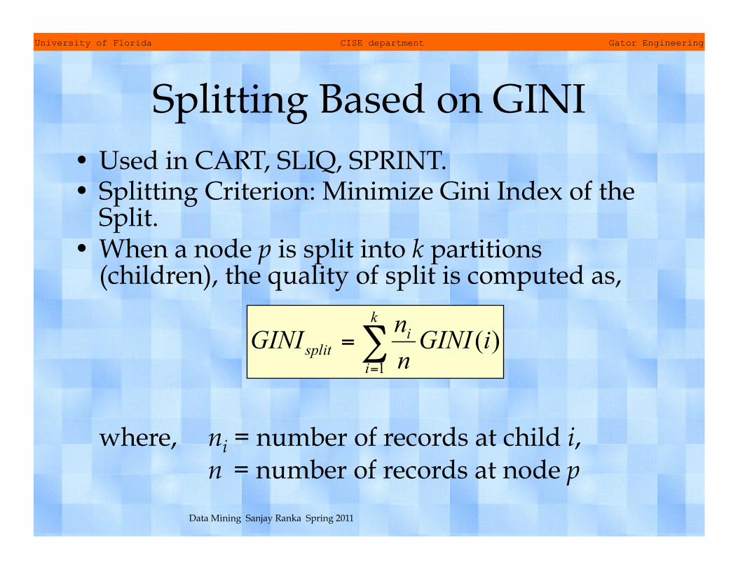
Splitting Based on GINI • Used in CART, SLIQ, SPRINT. • Splitting Criterion: Minimize Gini Index of the

Split. • When a node p is split into k partitions

(children), the quality of split is computed as,

where, ni = number of records at child i, n = number of records at node p



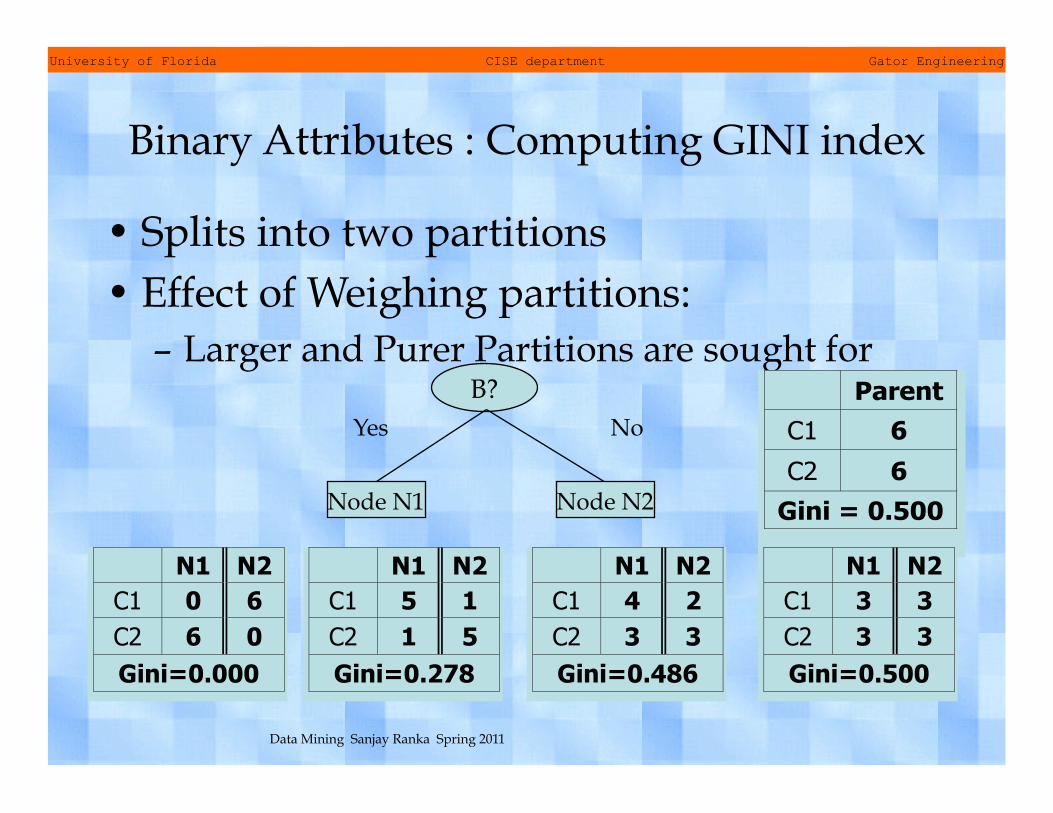
Binary Attributes : Computing GINI index

• Splits into two partitions • Effect of Weighing partitions:

– Larger and Purer Partitions are sought for B?

Yes No

Node N1 Node N2



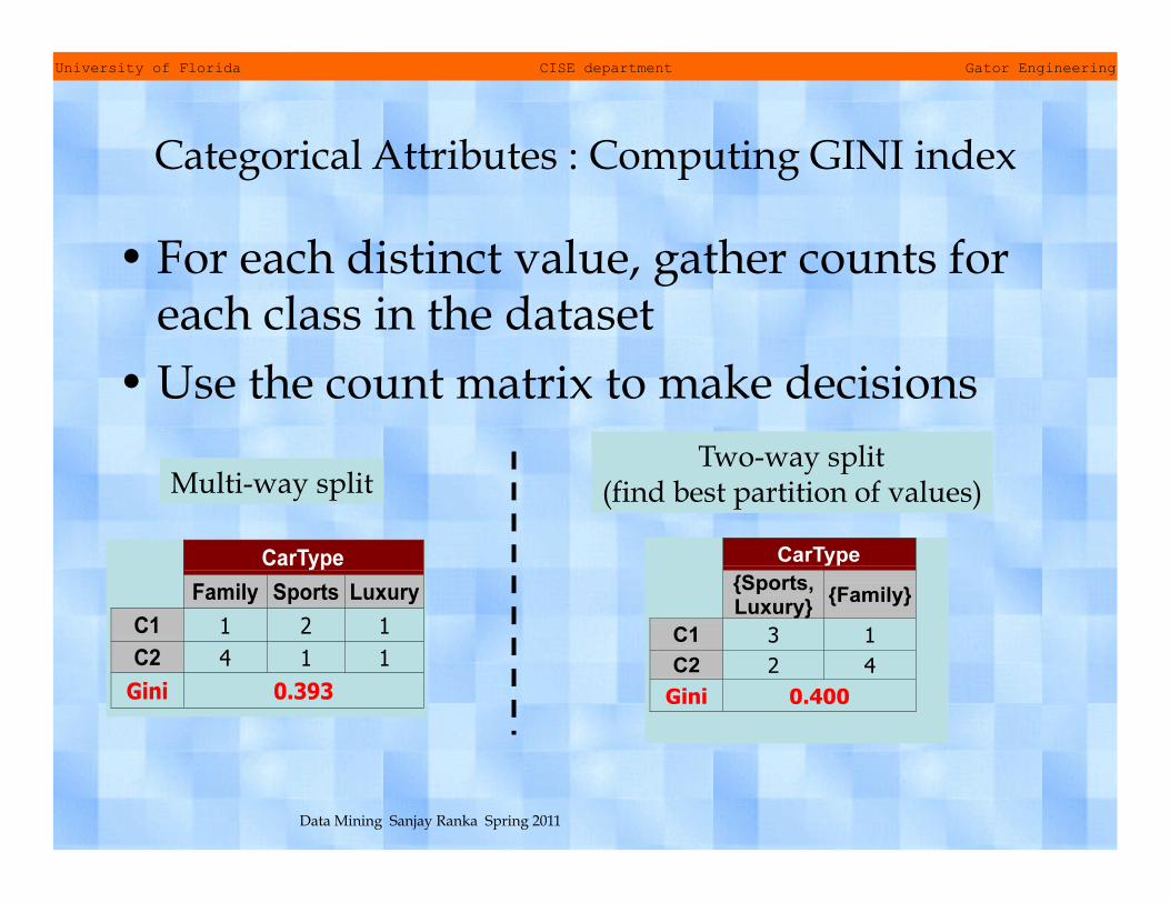
Categorical Attributes : Computing GINI index

• For each distinct value, gather counts for each class in the dataset

• Use the count matrix to make decisions

Multi-way split Two-way split

(find best partition of values)



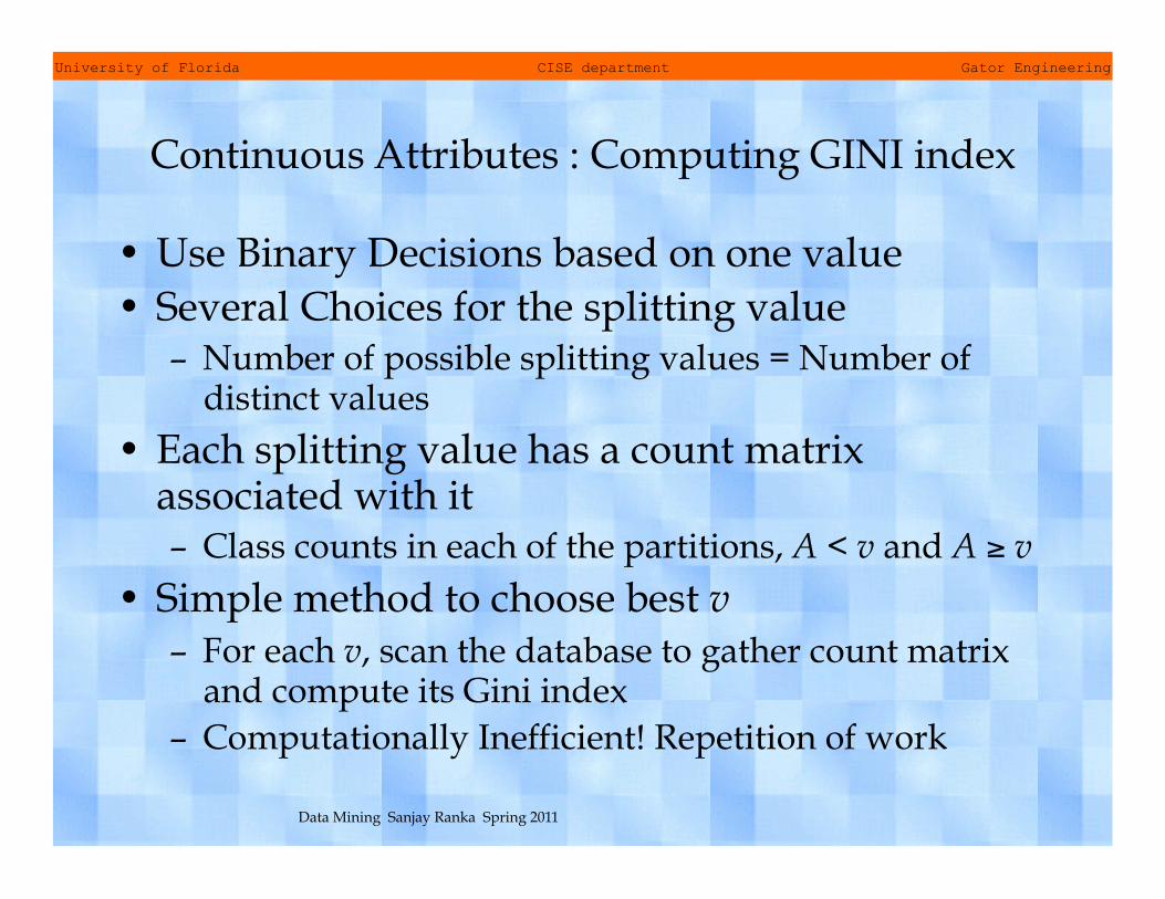
Continuous Attributes : Computing GINI index

• Use Binary Decisions based on one value • Several Choices for the splitting value

– Number of possible splitting values = Number of distinct values

• Each splitting value has a count matrix associated with it – Class counts in each of the partitions, A < v and A ≥ v

• Simple method to choose best v – For each v, scan the database to gather count matrix

and compute its Gini index – Computationally Inefficient! Repetition of work



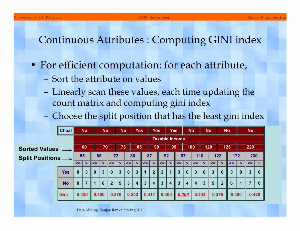
Continuous Attributes : Computing GINI index

• For efficient computation: for each attribute, – Sort the attribute on values – Linearly scan these values, each time updating the

count matrix and computing gini index – Choose the split position that has the least gini index

Split Positions Sorted Values



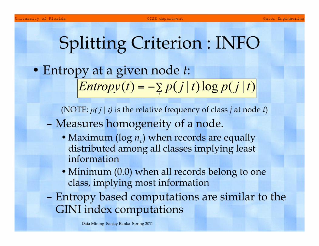
Splitting Criterion : INFO • Entropy at a given node t:

(NOTE: p( j | t) is the relative frequency of class j at node t) – Measures homogeneity of a node.

• Maximum (log nc) when records are equally distributed among all classes implying least information

• Minimum (0.0) when all records belong to one class, implying most information

– Entropy based computations are similar to the GINI index computations



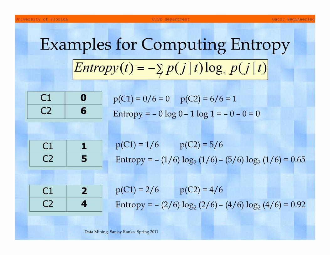
Examples for Computing Entropy

p(C1) = 0/6 = 0 p(C2) = 6/6 = 1

Entropy = – 0 log 0 – 1 log 1 = – 0 – 0 = 0

p(C1) = 1/6 p(C2) = 5/6

Entropy = – (1/6) log2 (1/6) – (5/6) log2 (1/6) = 0.65

p(C1) = 2/6 p(C2) = 4/6

Entropy = – (2/6) log2 (2/6) – (4/6) log2 (4/6) = 0.92



Splitting Based on INFO • Information Gain:

Parent Node, p is split into k partitions; ni is number of records in partition i

– Measures Reduction in Entropy achieved because of the split. Choose the split that achieves most reduction (maximizes GAIN)

– Used in ID3 and C4.5 – Disadvantage: Tends to prefer splits that result in

large number of partitions, each being small but pure



Splitting Based on INFO • Gain Ratio:

Parent Node, p is split into k partitions ni is the number of records in partition i

– Adjusts Information Gain by the entropy of the partitioning (SplitINFO). Higher entropy partitioning (large number of small partitions) is penalized!

– Used in C4.5 – Designed to overcome the disadvantage of

Information Gain



Splitting Criterion : Classification Error

• Classification error at a node t :

• Measures misclassification error made by a node – Maximum (1 - 1/nc) when records are equally

distributed among all classes, implying least interesting information

– Minimum (0.0) when all records belong to one class, implying most interesting information



Examples of Computing Classification Error

p(C1) = 0/6 = 0 p(C2) = 6/6 = 1

Error = 1 – max (0, 1) = 1 – 1 = 0

p(C1) = 1/6 p(C2) = 5/6

Error = 1 – max (1/6, 5/6) = 1 – 5/6 = 1/6

p(C1) = 2/6 p(C2) = 4/6

Error = 1 – max (2/6, 4/6) = 1 – 4/6 = 1/3



Comparison Among Splitting Criteria

• For a 2-class problem:



Practical Challenges in Classification

• Over-fitting – Model performs well on training set, but

poorly on test set

• Missing Values • Data Heterogeneity • Costs

– Costs for measuring attributes – Costs for misclassification



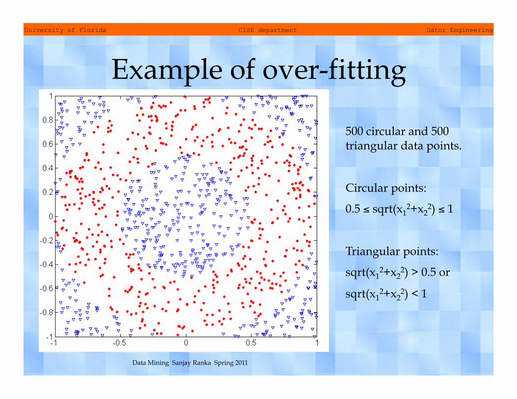
Example of over-fitting

500 circular and 500 triangular data points.

Circular points:

0.5 ≤ sqrt(x12+x2

2) ≤ 1

Triangular points:

sqrt(x12+x2

2) > 0.5 or

sqrt(x12+x2

2) < 1



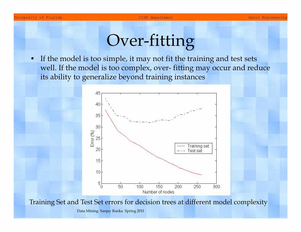
Over-fitting • If the model is too simple, it may not fit the training and test sets

well. If the model is too complex, over- fitting may occur and reduce its ability to generalize beyond training instances

Training Set and Test Set errors for decision trees at different model complexity



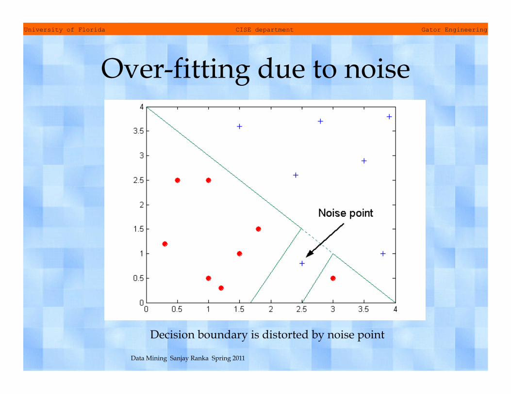
Over-fitting due to noise

Decision boundary is distorted by noise point



Over-fitting Due to Insufficient Training

Insufficient number of training points may cause the decision boundary to change



Estimating Generalization Error • Re-substitution errors: error on training (Σ e(t) ) • Generalization errors: error on testing (Σ e’(t))

• Method for estimating generalization errors: – Optimistic approach: e’(t) = e(t) – Pessimistic approach:

• For each leaf node: e’(t) = (e(t)+0.5) • Total errors: e’(T) = e(T) + N/2 (N: number of leaf nodes) • For a tree with 30 leaf nodes and 10 errors on training (out

of 1000 instances): – Training error = 10/1000 = 1% – Generalization error = (10 + 30×0.5)/1000 = 2.5%

– Reduced error pruning (REP): • uses validation data set to estimate generalization error



Occam’s Razor • Given two models of similar

generalization errors, one should prefer the simpler model over the more complex model

• For complex models, there is a greater chance that it was fitted accidentally by the data

• Therefore, one should include model complexity when evaluating a model



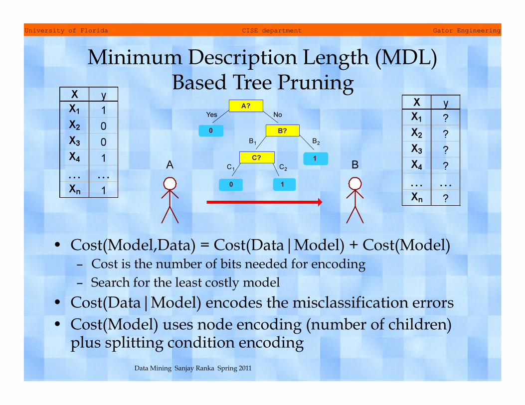
Minimum Description Length (MDL) Based Tree Pruning

• Cost(Model,Data) = Cost(Data|Model) + Cost(Model) – Cost is the number of bits needed for encoding – Search for the least costly model

• Cost(Data|Model) encodes the misclassification errors • Cost(Model) uses node encoding (number of children)

plus splitting condition encoding



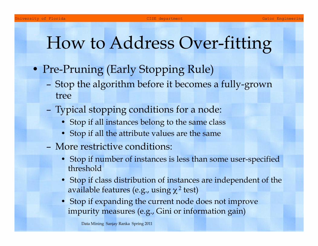
How to Address Over-fitting • Pre-Pruning (Early Stopping Rule)

– Stop the algorithm before it becomes a fully-grown tree

– Typical stopping conditions for a node: • Stop if all instances belong to the same class • Stop if all the attribute values are the same

– More restrictive conditions: • Stop if number of instances is less than some user-specified

threshold • Stop if class distribution of instances are independent of the

available features (e.g., using χ 2 test)

• Stop if expanding the current node does not improve impurity measures (e.g., Gini or information gain)



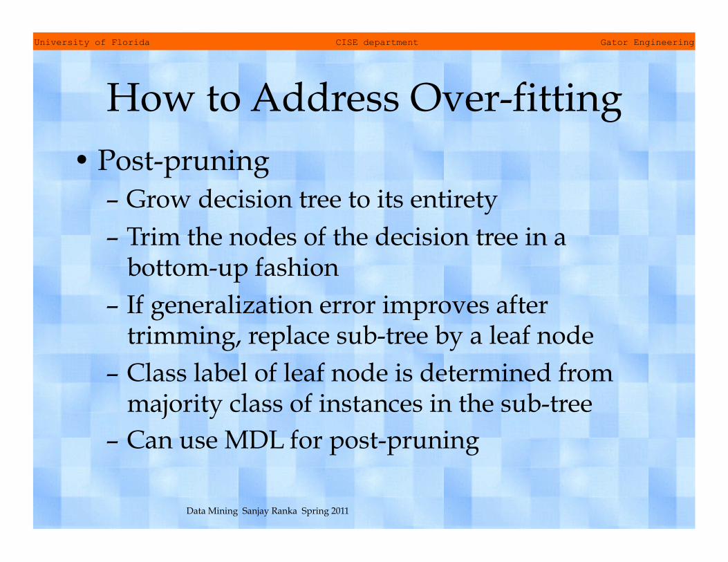
How to Address Over-fitting • Post-pruning

– Grow decision tree to its entirety – Trim the nodes of the decision tree in a

bottom-up fashion – If generalization error improves after

trimming, replace sub-tree by a leaf node – Class label of leaf node is determined from

majority class of instances in the sub-tree – Can use MDL for post-pruning



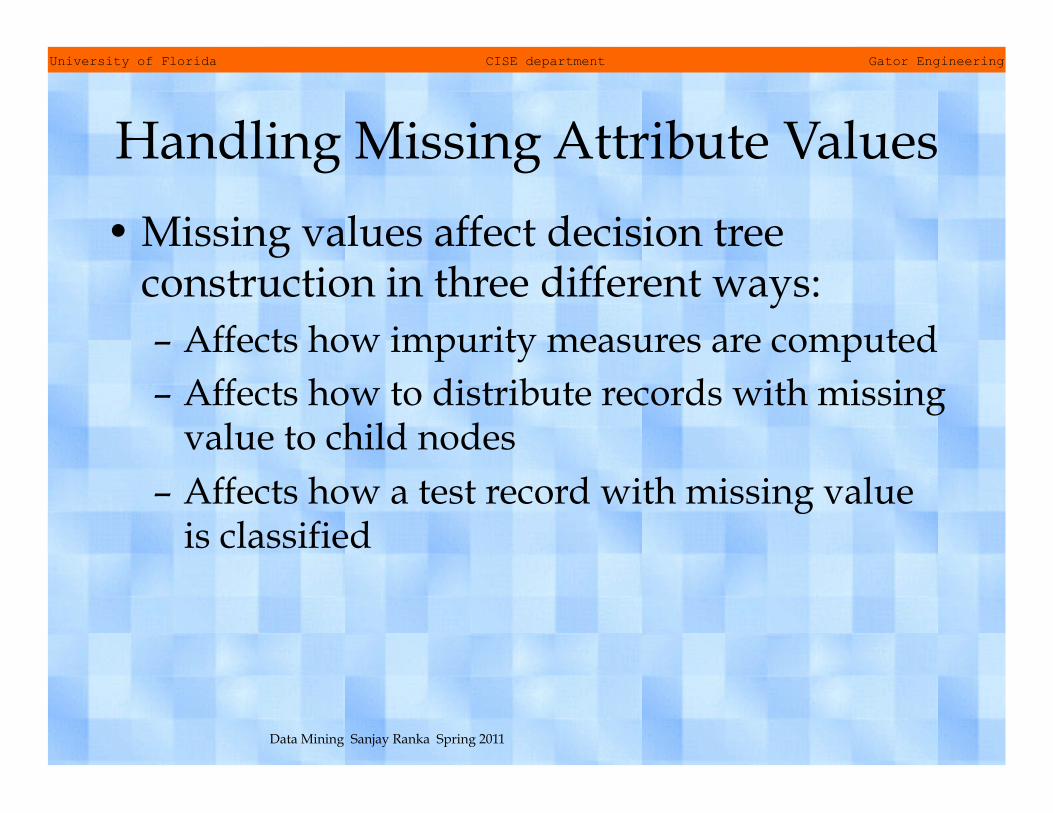
Handling Missing Attribute Values

• Missing values affect decision tree construction in three different ways: – Affects how impurity measures are computed – Affects how to distribute records with missing

value to child nodes – Affects how a test record with missing value

is classified



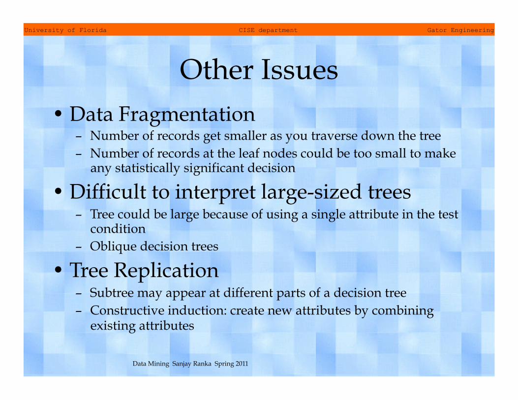
Other Issues • Data Fragmentation

– Number of records get smaller as you traverse down the tree – Number of records at the leaf nodes could be too small to make

any statistically significant decision

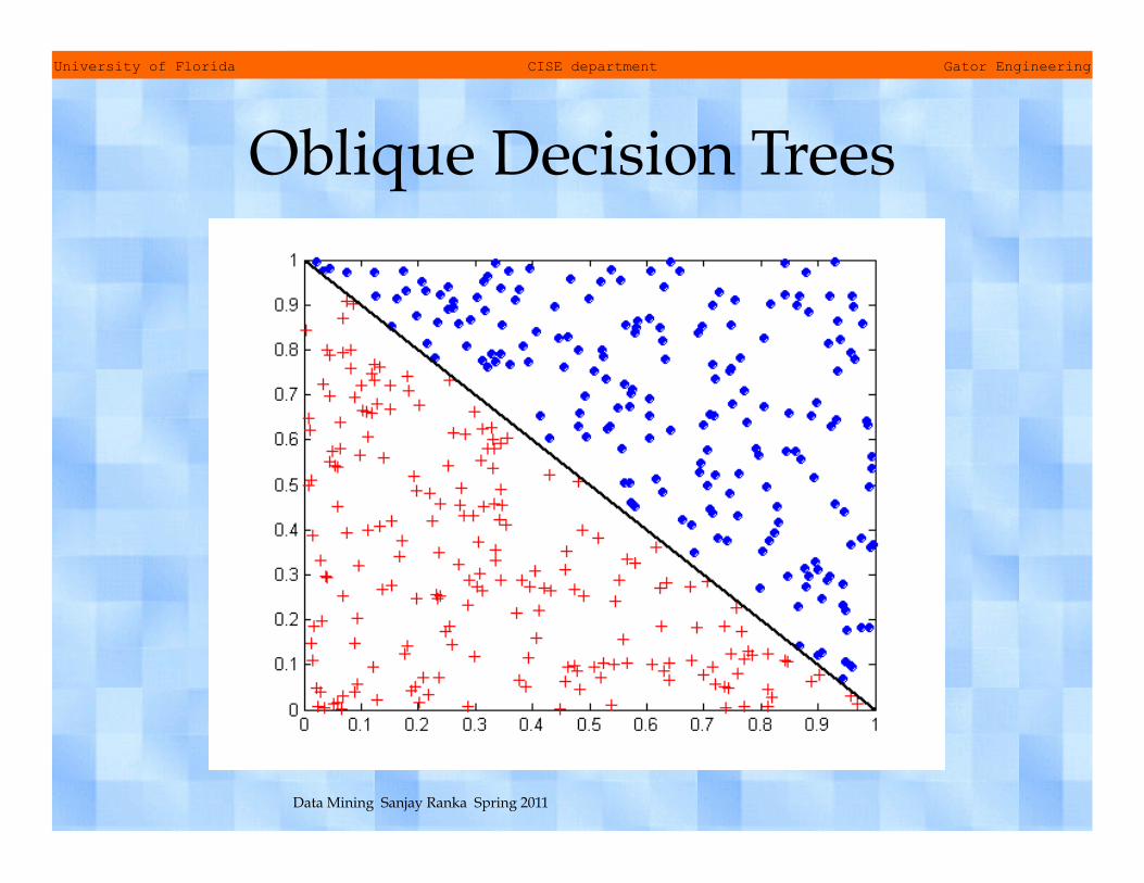
• Difficult to interpret large-sized trees – Tree could be large because of using a single attribute in the test

condition – Oblique decision trees

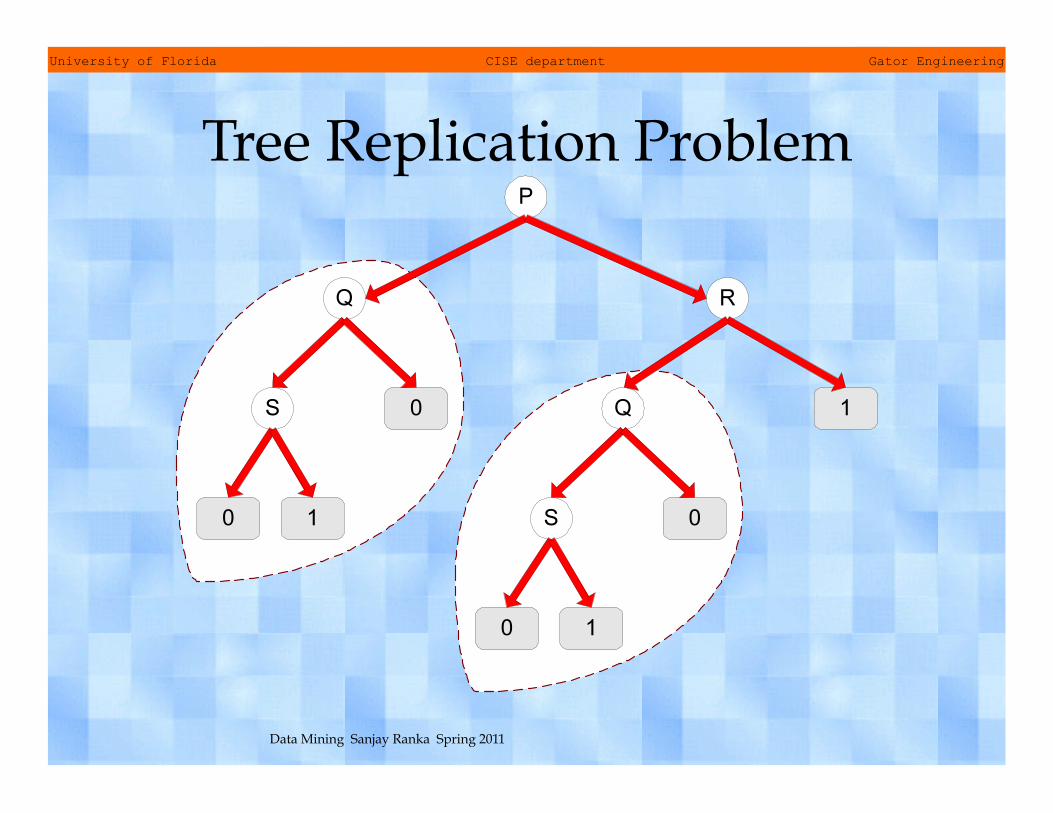
• Tree Replication – Subtree may appear at different parts of a decision tree – Constructive induction: create new attributes by combining

existing attributes



Oblique Decision Trees



Tree Replication Problem

Documents

Classification - Department of Computer and Information Science