Embed Size (px)
Citation preview

Classification: Basic Concepts and Decision Trees
A programming task

Classification: Definition Given a collection of records (training set )
Each record contains a set of attributes, one of the attributes is the class.
Find a model for class attribute as a function of the values of other attributes.
Goal: previously unseen records should be assigned a class as accurately as possible. A test set is used to determine the accuracy of the
model. Usually, the given data set is divided into training and test sets, with training set used to build the model and test set used to validate it.

Illustrating Classification Task
Apply Model
Induction
Deduction
Learn Model
Model
Tid Attrib1 Attrib2 Attrib3 Class
1 Yes Large 125K No
2 No Medium 100K No
3 No Small 70K No
4 Yes Medium 120K No
5 No Large 95K Yes
6 No Medium 60K No
7 Yes Large 220K No
8 No Small 85K Yes
9 No Medium 75K No
10 No Small 90K Yes 10
Tid Attrib1 Attrib2 Attrib3 Class
11 No Small 55K ?
12 Yes Medium 80K ?
13 Yes Large 110K ?
14 No Small 95K ?
15 No Large 67K ? 10
Test Set
Learningalgorithm
Training Set

Examples of Classification Task Predicting tumor cells as benign or malignant
Classifying credit card transactions as legitimate or fraudulent
Classifying secondary structures of protein as alpha-helix, beta-sheet, or random coil
Categorizing news stories as finance, weather, entertainment, sports, etc
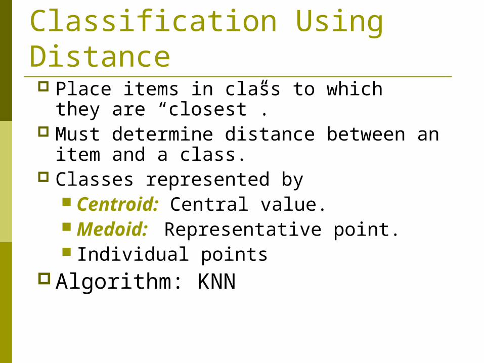
Classification Using Distance Place items in class to which they are
“closest”. Must determine distance between an
item and a class. Classes represented by
Centroid: Central value. Medoid: Representative point. Individual points
Algorithm: KNN

K Nearest Neighbor (KNN): Training set includes classes. Examine K items near item to be
classified. New item placed in class with the most
number of close items. O(q) for each tuple to be classified.
(Here q is the size of the training set.)

KNN

Classification Techniques Decision Tree based Methods Rule-based Methods Memory based reasoning Neural Networks Naïve Bayes and Bayesian Belief Networks Support Vector Machines

Example of a Decision Tree
Tid Refund MaritalStatus
TaxableIncome Cheat
1 Yes Single 125K No
2 No Married 100K No
3 No Single 70K No
4 Yes Married 120K No
5 No Divorced 95K Yes
6 No Married 60K No
7 Yes Divorced 220K No
8 No Single 85K Yes
9 No Married 75K No
10 No Single 90K Yes10
categorical
categorical
continuous
class
Refund
MarSt
TaxInc
YESNO
NO
NO
Yes No
Married Single, Divorced
< 80K > 80K
Splitting Attributes
Training Data Model: Decision Tree

Another Example of Decision Tree
Tid Refund MaritalStatus
TaxableIncome Cheat
1 Yes Single 125K No
2 No Married 100K No
3 No Single 70K No
4 Yes Married 120K No
5 No Divorced 95K Yes
6 No Married 60K No
7 Yes Divorced 220K No
8 No Single 85K Yes
9 No Married 75K No
10 No Single 90K Yes10
categorical
categorical
continuous
classMarSt
Refund
TaxInc
YESNO
NO
NO
Yes No
Married Single,
Divorced
< 80K > 80K
There could be more than one tree that fits the same data!

Decision Tree Classification Task
Apply Model
Induction
Deduction
Learn Model
Model
Tid Attrib1 Attrib2 Attrib3 Class
1 Yes Large 125K No
2 No Medium 100K No
3 No Small 70K No
4 Yes Medium 120K No
5 No Large 95K Yes
6 No Medium 60K No
7 Yes Large 220K No
8 No Small 85K Yes
9 No Medium 75K No
10 No Small 90K Yes 10
Tid Attrib1 Attrib2 Attrib3 Class
11 No Small 55K ?
12 Yes Medium 80K ?
13 Yes Large 110K ?
14 No Small 95K ?
15 No Large 67K ? 10
Test Set
TreeInductionalgorithm
Training SetDecision Tree
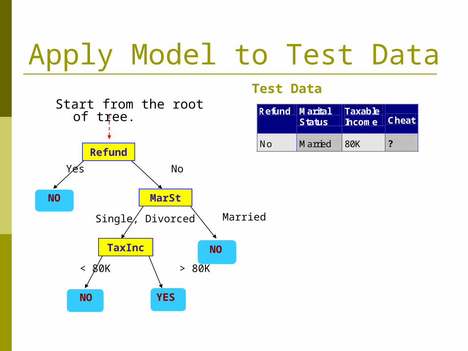
Apply Model to Test Data
Refund
MarSt
TaxInc
YESNO
NO
NO
Yes No
Married Single, Divorced
< 80K > 80K
Refund Marital Status
Taxable Income Cheat
No Married 80K ? 10
Test DataStart from the root of tree.

Apply Model to Test Data
Refund
MarSt
TaxInc
YESNO
NO
NO
Yes No
Married Single, Divorced
< 80K > 80K
Refund Marital Status
Taxable Income Cheat
No Married 80K ? 10
Test Data

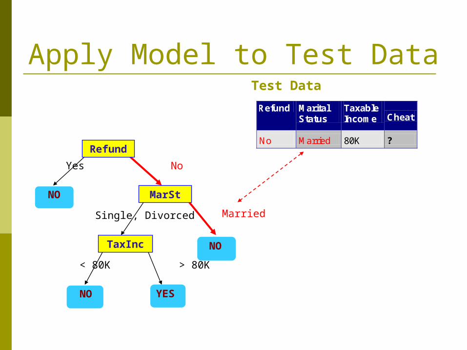
Apply Model to Test Data
Refund
MarSt
TaxInc
YESNO
NO
NO
Yes No
Married Single, Divorced
< 80K > 80K
Refund Marital Status
Taxable Income Cheat
No Married 80K ? 10
Test Data

Apply Model to Test Data
Refund
MarSt
TaxInc
YESNO
NO
NO
Yes No
Married Single, Divorced
< 80K > 80K
Refund Marital Status
Taxable Income Cheat
No Married 80K ? 10
Test Data
Apply Model to Test Data
Refund
MarSt
TaxInc
YESNO
NO
NO
Yes No
Married Single, Divorced
< 80K > 80K
Refund Marital Status
Taxable Income Cheat
No Married 80K ? 10
Test Data

Apply Model to Test Data
Refund
MarSt
TaxInc
YESNO
NO
NO
Yes No
Married Single, Divorced
< 80K > 80K
Refund Marital Status
Taxable Income Cheat
No Married 80K ? 10
Test Data
Assign Cheat to “No”

Decision Tree Classification Task
Apply Model
Induction
Deduction
Learn Model
Model
Tid Attrib1 Attrib2 Attrib3 Class
1 Yes Large 125K No
2 No Medium 100K No
3 No Small 70K No
4 Yes Medium 120K No
5 No Large 95K Yes
6 No Medium 60K No
7 Yes Large 220K No
8 No Small 85K Yes
9 No Medium 75K No
10 No Small 90K Yes 10
Tid Attrib1 Attrib2 Attrib3 Class
11 No Small 55K ?
12 Yes Medium 80K ?
13 Yes Large 110K ?
14 No Small 95K ?
15 No Large 67K ? 10
Test Set
TreeInductionalgorithm
Training Set
Decision Tree

Decision Tree Induction Many Algorithms:
Hunt’s Algorithm (one of the earliest) CART ID3, C4.5 SLIQ,SPRINT

General Structure of Hunt’s Algorithm Let Dt be the set of training
records that reach a node t General Procedure:
If Dt contains records that belong the same class yt, then t is a leaf node labeled as yt
If Dt is an empty set, then t is a leaf node labeled by the default class, yd
If Dt contains records that belong to more than one class, use an attribute test to split the data into smaller subsets. Recursively apply the procedure to each subset.
Tid Refund Marital Status
Taxable Income Cheat
1 Yes Single 125K No
2 No Married 100K No
3 No Single 70K No
4 Yes Married 120K No
5 No Divorced 95K Yes
6 No Married 60K No
7 Yes Divorced 220K No
8 No Single 85K Yes
9 No Married 75K No
10 No Single 90K Yes 10
Dt
?

Hunt’s AlgorithmDon’t Cheat
Refund
Don’t Cheat
Don’t Cheat
Yes No
Refund
Don’t Cheat
Yes No
MaritalStatus
Don’t Cheat
Cheat
Single,Divorced Married
TaxableIncome
Don’t Cheat
< 80K >= 80K
Refund
Don’t Cheat
Yes No
MaritalStatus
Don’t Cheat
Cheat
Single,Divorced Married

Tree Induction Greedy strategy.
Split the records based on an attribute test that optimizes certain criterion.
Issues Determine how to split the records
How to specify the attribute test condition? How to determine the best split?
Determine when to stop splitting

Tree Induction Greedy strategy.
Split the records based on an attribute test that optimizes certain criterion.
Issues Determine how to split the records
How to specify the attribute test condition? How to determine the best split?
Determine when to stop splitting

How to Specify Test Condition? Depends on attribute types
Nominal Ordinal Continuous
Depends on number of ways to split 2-way split Multi-way split

Splitting Based on Nominal Attributes Multi-way split: Use as many partitions as distinct
values.
Binary split: Divides values into two subsets. Need to find optimal partitioning.
CarTypeFamily
SportsLuxury
CarType{Family, Luxury} {Sports}
CarType{Sports, Luxury} {Family}
OR
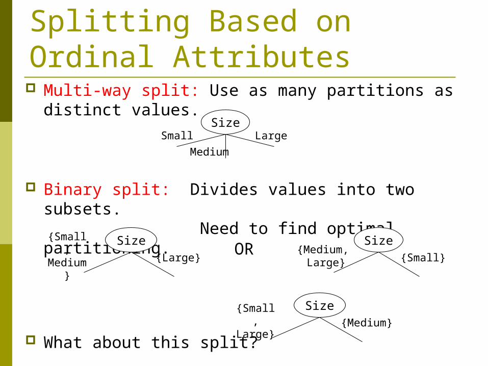
Multi-way split: Use as many partitions as distinct values.
Binary split: Divides values into two subsets. Need to find optimal partitioning.
What about this split?
Splitting Based on Ordinal Attributes
SizeSmall
MediumLarge
Size{Medium,
Large} {Small}Size
{Small, Medium} {Large} OR
Size{Small, Large} {Medium}

Splitting Based on Continuous Attributes Different ways of handling
Discretization to form an ordinal categorical attribute
Static – discretize once at the beginning Dynamic – ranges can be found by equal interval
bucketing, equal frequency bucketing
(percentiles), or clustering.
Binary Decision: (A < v) or (A v) consider all possible splits and finds the best cut can be more compute intensive
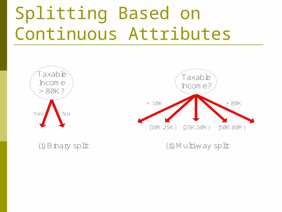
Splitting Based on Continuous Attributes
TaxableIncome> 80K?
Yes No
TaxableIncome?
(i) Binary split (ii) Multi-way split
< 10K
[10K,25K) [25K,50K) [50K,80K)
> 80K

Tree Induction Greedy strategy.
Split the records based on an attribute test that optimizes certain criterion.
Issues Determine how to split the records
How to specify the attribute test condition? How to determine the best split?
Determine when to stop splitting
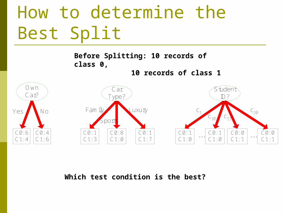
How to determine the Best Split
OwnCar?
C0: 6C1: 4
C0: 4C1: 6
C0: 1C1: 3
C0: 8C1: 0
C0: 1C1: 7
CarType?
C0: 1C1: 0
C0: 1C1: 0
C0: 0C1: 1
StudentID?
...
Yes No Family
Sports
Luxury c1c10
c20
C0: 0C1: 1
...
c11
Before Splitting: 10 records of class 0,10 records of class 1
Which test condition is the best?

How to determine the Best Split Greedy approach:
Nodes with homogeneous class distribution are preferred
Need a measure of node impurity:
C0: 5C1: 5
C0: 9C1: 1
Non-homogeneous,
High degree of impurity
Homogeneous,
Low degree of impurity

Measures of Node Impurity Gini Index
Entropy
Misclassification error

How to Find the Best Split
B?
Yes No
Node N3 Node N4
A?
Yes No
Node N1 Node N2
Before Splitting:
C0 N10 C1 N11
C0 N20 C1 N21
C0 N30 C1 N31
C0 N40 C1 N41
C0 N00 C1 N01
M0
M1 M2 M3 M4
M12 M34Gain = M0 – M12 vs M0 – M34

Measure of Impurity: GINI Gini Index for a given node t :
(NOTE: p( j | t) is the relative frequency of class j at node t). Maximum (1 - 1/nc) when records are equally distributed
among all classes, implying least interesting information Minimum (0.0) when all records belong to one class,
implying most interesting information
j
tjptGINI 2)]|([1)(
C1 0C2 6
Gini=0.000
C1 2C2 4
Gini=0.444
C1 3C2 3
Gini=0.500
C1 1C2 5
Gini=0.278
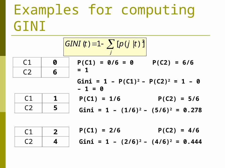
Examples for computing GINI
C1 0 C2 6
C1 2 C2 4
C1 1 C2 5
P(C1) = 0/6 = 0 P(C2) = 6/6 = 1
Gini = 1 – P(C1)2 – P(C2)2 = 1 – 0 – 1 = 0
j
tjptGINI 2)]|([1)(
P(C1) = 1/6 P(C2) = 5/6
Gini = 1 – (1/6)2 – (5/6)2 = 0.278
P(C1) = 2/6 P(C2) = 4/6
Gini = 1 – (2/6)2 – (4/6)2 = 0.444

Splitting Based on GINI Used in CART, SLIQ, SPRINT. When a node p is split into k partitions (children),
the quality of split is computed as,
where, ni = number of records at child i, n = number of records at node
p.
k
i
isplit iGINI
nnGINI
1
)(
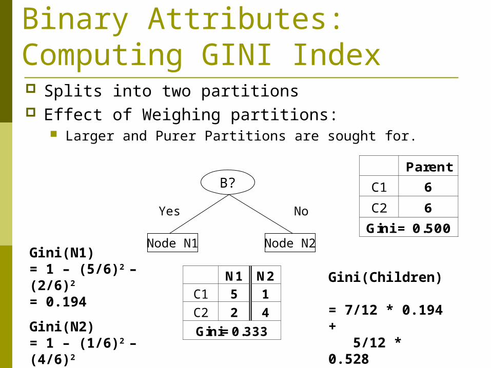
Binary Attributes: Computing GINI Index Splits into two partitions Effect of Weighing partitions:
Larger and Purer Partitions are sought for.
B?
Yes No
Node N1 Node N2
Parent C1 6 C2 6
Gini = 0.500
N1 N2 C1 5 1 C2 2 4 Gini=0.333
Gini(N1) = 1 – (5/6)2 – (2/6)2 = 0.194
Gini(N2) = 1 – (1/6)2 – (4/6)2 = 0.528
Gini(Children) = 7/12 * 0.194 + 5/12 * 0.528= 0.333

Categorical Attributes: Computing Gini Index For each distinct value, gather counts for each
class in the dataset Use the count matrix to make decisions
CarType{Sports,Luxury} {Family}
C1 3 1C2 2 4
Gini 0.400
CarType
{Sports} {Family,Luxury}
C1 2 2C2 1 5
Gini 0.419
CarTypeFamily Sports Luxury
C1 1 2 1C2 4 1 1
Gini 0.393
Multi-way split Two-way split (find best partition of values)
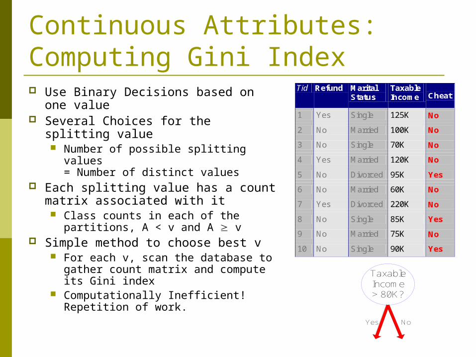
Continuous Attributes: Computing Gini Index Use Binary Decisions based on one
value Several Choices for the splitting
value Number of possible splitting values
= Number of distinct values Each splitting value has a count
matrix associated with it Class counts in each of the
partitions, A < v and A v Simple method to choose best v
For each v, scan the database to gather count matrix and compute its Gini index
Computationally Inefficient! Repetition of work.
TaxableIncome> 80K?
Yes No
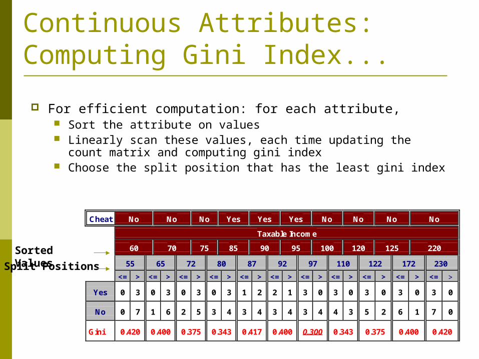
Continuous Attributes: Computing Gini Index...
For efficient computation: for each attribute, Sort the attribute on values Linearly scan these values, each time updating the count
matrix and computing gini index Choose the split position that has the least gini index
Cheat No No No Yes Yes Yes No No No No
Taxable Income
60 70 75 85 90 95 100 120 125 220
55 65 72 80 87 92 97 110 122 172 230<= > <= > <= > <= > <= > <= > <= > <= > <= > <= > <= >
Yes 0 3 0 3 0 3 0 3 1 2 2 1 3 0 3 0 3 0 3 0 3 0
No 0 7 1 6 2 5 3 4 3 4 3 4 3 4 4 3 5 2 6 1 7 0
Gini 0.420 0.400 0.375 0.343 0.417 0.400 0.300 0.343 0.375 0.400 0.420
Split PositionsSorted Values

Alternative Splitting Criteria based on INFO
Entropy at a given node t:
(NOTE: p( j | t) is the relative frequency of class j at node t). Measures homogeneity of a node.
Maximum (log nc) when records are equally distributed among all classes implying least information
Minimum (0.0) when all records belong to one class, implying most information
Entropy based computations are similar to the GINI index computations
j
tjptjptEntropy )|(log)|()(

Examples for computing Entropy
C1 0 C2 6
C1 2 C2 4
C1 1 C2 5
P(C1) = 0/6 = 0 P(C2) = 6/6 = 1
Entropy = – 0 log 0 – 1 log 1 = – 0 – 0 = 0
P(C1) = 1/6 P(C2) = 5/6
Entropy = – (1/6) log2 (1/6) – (5/6) log2 (1/6) = 0.65
P(C1) = 2/6 P(C2) = 4/6
Entropy = – (2/6) log2 (2/6) – (4/6) log2 (4/6) = 0.92
j
tjptjptEntropy )|(log)|()(2

Splitting Based on INFO... Information Gain:
Parent Node, p is split into k partitions;ni is number of records in partition i
Measures Reduction in Entropy achieved because of the split. Choose the split that achieves most reduction (maximizes GAIN)
Used in ID3 and C4.5 Disadvantage: Tends to prefer splits that result in large
number of partitions, each being small but pure.
k
i
i
splitiEntropy
nnpEntropyGAIN
1)()(

Splitting Based on INFO... Gain Ratio:
Parent Node, p is split into k partitionsni is the number of records in partition i
Adjusts Information Gain by the entropy of the partitioning (SplitINFO). Higher entropy partitioning (large number of small partitions) is penalized!
Used in C4.5 Designed to overcome the disadvantage of Information
Gain
SplitINFOGAIN
GainRATIO Split
split
k
i
ii
nn
nnSplitINFO
1log

Splitting Criteria based on Classification Error Classification error at a node t :
Measures misclassification error made by a node. Maximum (1 - 1/nc) when records are equally distributed
among all classes, implying least interesting information Minimum (0.0) when all records belong to one class,
implying most interesting information
)|(max1)( tiPtErrori

Examples for Computing Error
C1 0 C2 6
C1 2 C2 4
C1 1 C2 5
P(C1) = 0/6 = 0 P(C2) = 6/6 = 1
Error = 1 – max (0, 1) = 1 – 1 = 0
P(C1) = 1/6 P(C2) = 5/6
Error = 1 – max (1/6, 5/6) = 1 – 5/6 = 1/6
P(C1) = 2/6 P(C2) = 4/6
Error = 1 – max (2/6, 4/6) = 1 – 4/6 = 1/3
)|(max1)( tiPtErrori

Comparison among Splitting CriteriaFor a 2-class problem:

Misclassification Error vs Gini
A?
Yes No
Node N1 Node N2
Parent C1 7 C2 3 Gini = 0.42
N1 N2 C1 3 4 C2 0 3
Gini(N1) = 1 – (3/3)2 – (0/3)2 = 0
Gini(N2) = 1 – (4/7)2 – (3/7)2 = 0.489
Gini(Children) = 3/10 * 0 + 7/10 * 0.489= 0.342

Tree Induction Greedy strategy.
Split the records based on an attribute test that optimizes certain criterion.
Issues Determine how to split the records
How to specify the attribute test condition? How to determine the best split?
Determine when to stop splitting

Stopping Criteria for Tree Induction Stop expanding a node when all the
records belong to the same class
Stop expanding a node when all the records have similar attribute values
Early termination (to be discussed later)

Decision Tree Based Classification Advantages:
Inexpensive to construct Extremely fast at classifying unknown records Easy to interpret for small-sized trees Accuracy is comparable to other classification
techniques for many simple data sets

Example: C4.5 Simple depth-first construction. Uses Information Gain Sorts Continuous Attributes at each node. Needs entire data to fit in memory. Unsuitable for Large Datasets.
Needs out-of-core sorting.
You can download the software from:http://www.cse.unsw.edu.au/~quinlan/c4.5r8.tar.gz

Practical Issues of Classification Underfitting and Overfitting
Missing Values
Costs of Classification

Underfitting and Overfitting (Example)
500 circular and 500 triangular data points.
Circular points:
0.5 sqrt(x12+x2
2) 1
Triangular points:
sqrt(x12+x2
2) > 0.5 or
sqrt(x12+x2
2) < 1

Underfitting and OverfittingOverfitting
Underfitting: when model is too simple, both training and test errors are large
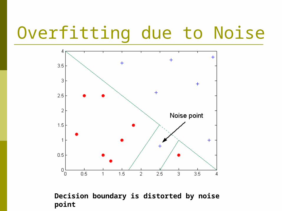
Overfitting due to Noise
Decision boundary is distorted by noise point

Overfitting due to Insufficient Examples
Lack of data points in the lower half of the diagram makes it difficult to predict correctly the class labels of that region
- Insufficient number of training records in the region causes the decision tree to predict the test examples using other training records that are irrelevant to the classification task

Notes on Overfitting Overfitting results in decision trees that
are more complex than necessary
Training error no longer provides a good estimate of how well the tree will perform on previously unseen records
Need new ways for estimating errors

Estimating Generalization Errors Re-substitution errors: error on training ( e(t) ) Generalization errors: error on testing ( e’(t)) Methods for estimating generalization errors:
Optimistic approach: e’(t) = e(t) Pessimistic approach:
For each leaf node: e’(t) = (e(t)+0.5) Total errors: e’(T) = e(T) + N 0.5 (N: number of leaf
nodes) For a tree with 30 leaf nodes and 10 errors on training
(out of 1000 instances): Training error = 10/1000 = 1%
Generalization error = (10 + 300.5)/1000 = 2.5% Reduced error pruning (REP):
uses validation data set to estimate generalization error
Occam’s Razor Given two models of similar generalization
errors, one should prefer the simpler model over the more complex model
For complex models, there is a greater chance that it was fitted accidentally by errors in data
Therefore, one should include model complexity when evaluating a model
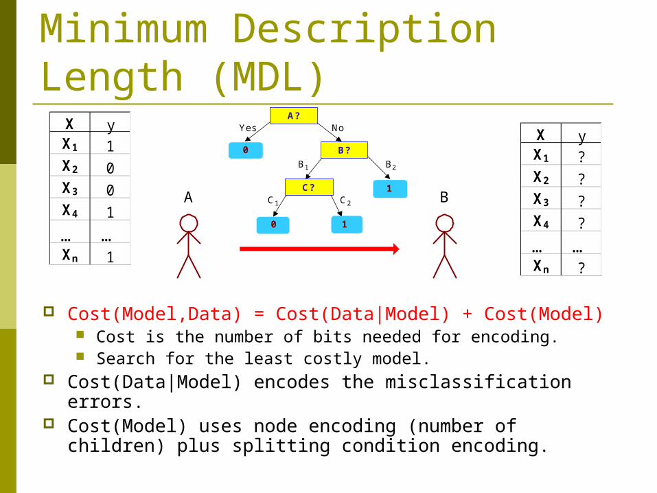
Minimum Description Length (MDL)
Cost(Model,Data) = Cost(Data|Model) + Cost(Model) Cost is the number of bits needed for encoding. Search for the least costly model.
Cost(Data|Model) encodes the misclassification errors. Cost(Model) uses node encoding (number of children) plus
splitting condition encoding.
A B
A?
B?
C?
10
0
1
Yes No
B1 B2
C1 C2
X yX1 1X2 0X3 0X4 1… …Xn 1
X yX1 ?X2 ?X3 ?X4 ?… …Xn ?

How to Address Overfitting Pre-Pruning (Early Stopping Rule)
Stop the algorithm before it becomes a fully-grown tree Typical stopping conditions for a node:
Stop if all instances belong to the same class Stop if all the attribute values are the same
More restrictive conditions: Stop if number of instances is less than some user-specified
threshold Stop if class distribution of instances are independent of the
available features (e.g., using 2 test) Stop if expanding the current node does not improve impurity
measures (e.g., Gini or information gain).
How to Address Overfitting… Post-pruning
Grow decision tree to its entirety Trim the nodes of the decision tree in a
bottom-up fashion If generalization error improves after trimming,
replace sub-tree by a leaf node. Class label of leaf node is determined from
majority class of instances in the sub-tree Can use MDL for post-pruning

Example of Post-Pruning
A?
A1
A2 A3
A4
Class = Yes 20Class = No 10
Error = 10/30
Training Error (Before splitting) = 10/30
Pessimistic error = (10 + 0.5)/30 = 10.5/30
Training Error (After splitting) = 9/30
Pessimistic error (After splitting)
= (9 + 4 0.5)/30 = 11/30
PRUNE!
Class = Yes
8
Class = No 4
Class = Yes
3
Class = No 4
Class = Yes
4
Class = No 1
Class = Yes
5
Class = No 1

Examples of Post-pruning Optimistic error?
Pessimistic error?
Reduced error pruning?
C0: 11C1: 3
C0: 2C1: 4
C0: 14C1: 3
C0: 2C1: 2
Don’t prune for both cases
Don’t prune case 1, prune case 2
Case 1:
Case 2:
Depends on validation set

Handling Missing Attribute Values Missing values affect decision tree
construction in three different ways: Affects how impurity measures are computed Affects how to distribute instance with missing
value to child nodes Affects how a test instance with missing value
is classified

Computing Impurity MeasureTid Refund Marital
Status Taxable Income Class
1 Yes Single 125K No
2 No Married 100K No
3 No Single 70K No
4 Yes Married 120K No
5 No Divorced 95K Yes
6 No Married 60K No
7 Yes Divorced 220K No
8 No Single 85K Yes
9 No Married 75K No
10 ? Single 90K Yes 10
Class = Yes
Class = No
Refund=Yes 0 3 Refund=No 2 4
Refund=? 1 0
Split on Refund:
Entropy(Refund=Yes) = 0
Entropy(Refund=No) = -(2/6)log(2/6) – (4/6)log(4/6) = 0.9183
Entropy(Children) = 0.3 (0) + 0.6 (0.9183) = 0.551
Gain = 0.9 (0.8813 – 0.551) = 0.3303
Missing value
Before Splitting: Entropy(Parent) = -0.3 log(0.3)-(0.7)log(0.7) = 0.8813

Distribute InstancesTid Refund Marital
Status Taxable Income Class
1 Yes Single 125K No
2 No Married 100K No
3 No Single 70K No
4 Yes Married 120K No
5 No Divorced 95K Yes
6 No Married 60K No
7 Yes Divorced 220K No
8 No Single 85K Yes
9 No Married 75K No 10
RefundYes No
Class=Yes 0 Class=No 3
Cheat=Yes 2 Cheat=No 4
RefundYes
Tid Refund Marital Status
Taxable Income Class
10 ? Single 90K Yes 10
No
Class=Yes 2 + 6/ 9 Class=No 4
Probability that Refund=Yes is 3/9
Probability that Refund=No is 6/9
Assign record to the left child with weight = 3/9 and to the right child with weight = 6/9
Class=Yes 0 + 3/ 9 Class=No 3

Classify Instances
Refund
MarSt
TaxInc
YESNO
NO
NO
Yes No
Married Single, Divorced
< 80K > 80K
Married Single Divorced
Total
Class=No 3 1 0 4
Class=Yes 6/9 1 1 2.67
Total 3.67 2 1 6.67
Tid Refund Marital Status
Taxable Income Class
11 No ? 85K ? 10
New record:
Probability that Marital Status = Married is 3.67/6.67
Probability that Marital Status ={Single,Divorced} is 3/6.67

Scalable Decision Tree Induction Methods
SLIQ (EDBT’96 — Mehta et al.) Builds an index for each attribute and only class list and the
current attribute list reside in memory SPRINT (VLDB’96 — J. Shafer et al.)
Constructs an attribute list data structure PUBLIC (VLDB’98 — Rastogi & Shim)
Integrates tree splitting and tree pruning: stop growing the tree earlier
RainForest (VLDB’98 — Gehrke, Ramakrishnan & Ganti) Builds an AVC-list (attribute, value, class label)
BOAT (PODS’99 — Gehrke, Ganti, Ramakrishnan & Loh) Uses bootstrapping to create several small samples