Embed Size (px)
Citation preview
Volume 2, Number 2, Pages 107–132ISSN 1715-0868
CLASS NUMBER APPROXIMATION IN CUBIC
FUNCTION FIELDS
RENATE SCHEIDLER AND ANDREAS STEIN
Abstract. We develop explicitly computable bounds for the order ofthe Jacobian of a cubic function field. We use approximations via trun-cated Euler products and thus derive effective methods of computing theorder of the Jacobian of a cubic function field. Also, a detailed discussionof the zeta function of a cubic function field extension is included.
1. Introduction and Motivation
A central problem in number theory and algebraic geometry is the de-termination of the size of the group of rational points on the Jacobian ofan algebraic curve over a finite field. This question also has applications tocryptography, since cryptographic systems based on algebraic curves gener-ally require a Jacobian of non-smooth order in order to foil certain types ofattacks.
There a variety of methods for accomplishing this task; some are general,while others are only applicable to specific types of curves. In the interestof space, we forego citing most the large volume of literature on elliptic andhyperelliptic curves in detail, and mention only two sources. Kedlaya’s p-adic algorithm for hyperelliptic curves [23, 24] is particularly well-suited tofields of small characteristic and has since been extended to Artin-Schreierextensions [14, 26, 27], superelliptic curves [17, 28], Cab curves [15], andmore general curves [18, 13]; see also the survey by Kelaya [25]. A verydifferent approach was first given by Schoof for elliptic curves [37]; thismethod was generalized to Abelian varieties by Pila [30, 31] and improvedby Adleman and Huang [1, 2]. The Adleman-Huang algorithm computesthe characteristic polynomial of the Frobenius endomorphism of an Abelianvariety of dimension d in projective N -space over a finite field Fq in time
O(log(q)δ) where δ depends polynomially on d and N . For plane curves
Received by the editors June 21, 2007, and in revised form September 13, 2007.1991 Mathematics Subject Classification. Primary 11R58, 11Y16. Secondary 11M38,
11R65,11R16.Key words and phrases. cubic function field, class number, regulator, truncated Euler
product.Research of the first author supported by NSERC of Canada.Research by the second author supported by NSF Grant DMS-0201337.
c©2007 University of Calgary
107
108 RENATE SCHEIDLER AND ANDREAS STEIN
of degree n, a randomized algorithm with running time O(log(q)nO(1)
) wasgiven by Hang and Ierardi [22].
We note that none of the last five citations above provides an imple-mentation or numerical data, so their practical effectiveness remains to beestablished. In fact, the method of [2] requires a semi-algebraic descrip-tion of the Jacobian as an algebraic variety, and while the authors illustratehow to obtain such a description for hyperelliptic curves from the Mumfordrepresentations of reduced divisors, this task can be complicated for moregeneral curves. On the other hand, methods for special types of curves haveyielded impressive results. The algorithm of [19] for genus 2 hyperellipticcurves, for example, produced class numbers of 39 decimal digits, and theimprovements of [20] pushed this up to the cryptographically secure rangeof 50 decimal digits (164 bits). In 2002, a class number of 29 digits for agenus 3 hyperelliptic curve was computed in [39]. The method for Picardcurves given in [4] generated prime class numbers of up to 39 decimal digitsas well as a 55-digit class number with a 52-digit (173 bit) prime factor.
In this paper, we develop explicit bounds on the divisor class numberh, i.e. the order of the Jacobian of a cubic extension K of a rational func-tion field Fq(X) of finite characteristic different from 3. More exactly, wedetermine a good approximation E and an accuracy measure L such that|h − E| < L2. In the case where the genus g of the extension is at most 2,the Hasse-Weil bound yields good choices for E and L. If g ≥ 3, then wefind better effective choices for E and L by making use of the Euler productrepresentation of the L-polynomial of K/Fq(X). In essence, E is obtainedby truncating this Euler product at some suitable point, and L is given bythe tail of the truncated Euler product. Here, the cut-off point for the Eulerproduct needs to be chosen in a way that minimizes the time required tofind h in the open interval ]E − L2, E + L2[.
Once E and L are determined, the actual value of h can subsequentlybe found by searching the open interval ]E − L2, E + L2[ using Shanks’baby step-giant step method or Pollard’s kangaroo method. The complexityof this search (in terms of multiplications and reductions on ideals in themaximal order of K/Fq(X)) is determined by the square root of the length
of the interval, i.e. O(√
2L2 − 1) = O(L), so the overall complexity of themethod is O(max{TE , L}), where TE denotes the time for computing theapproximation E. For small genus g, the Hasse-Weil bound yields runningtimes of O(q1/4) for g = 1 and O(q3/4) for g = 2, while for g ≥ 3, we obtain
a running time of essentially O(q(2g−1)/5) as q grows.The above technique for finding E and L was first introduced in [41]
where it was used to bound the class number of a hyperelliptic functionfield of odd characteristic and arbitrary genus. It was applied to generatingclass numbers of hyperelliptic curves using an optimized baby step-giantstep search in [40] and a parallelized version of Pollard’s kangaroo methodin [39]; as mentioned earlier, the latter produced class numbers in excess of
CLASS NUMBER APPROXIMATION IN CUBIC FUNCTION FIELDS 109
1028 with computer technology dating from before 2002. Given the successin generating large numerical examples in the hyperelliptic scenario, themethod seemed a promising candidate for generalization to cubic and othertypes of function fields. While the basic idea is the same for both thehyperelliptic and the cubic case, the actual realization of the bounds issignificantly more complicated in the latter scenario. In fact, the methodcan be used for any function field extension K/Fq(X), but the derivationof explicit values for E and L becomes increasingly more complicated asthe degree of the extension — and thus the number of possibilities for thesplitting behavior in K of the places of Fq(X) — grows.
The emphasis and scope of this article is the development of precise for-mulae for the quantities E and L for a cubic extension K/Fq(X). In thecase where the extension is purely cubic, i.e. K = Fq(X,Y ) with Y 3 ∈ Fq[X]a cube-free polynomial, we also provide algorithms for explicitly calculat-ing the relevant character that appears in these formulae. We defer theimplementation and the actual computation of the divisor class number h,including the generation of numerical data, to a future paper.
We now proceed as follows. We begin by summarizing results on curvesand (cubic) function fields in Section 2. Section 3 describes the idea of thealgorithms. In Section 4, we develop results on the zeta function of a cubicfunction field and prove our main theorems. In Section 5, we apply theseresults to cubic function fields and discuss two choices for E and L, derivingexplicit bounds for both choices as well. This section also includes a com-plexity analysis of our algorithms. In Section 6, we study the computationof the dth power residue symbol that is needed in our algorithms. We finishour paper with open problems and future research topics.
2. Curves and Function Fields
2.1. Notation and Definitions. For a general overview of function fields,we refer to [32, 42]. Let K/k with k = Fq be an algebraic function field ofgenus g where q is a prime power, and let X ∈ K be transcendental over k,so that K/k(X) is a finite separable extension of degree m. We assume thatgcd(q,m) = 1. We can write K = k(X,Y ) with F (X,Y ) = 0 where F (X,Y )is an absolutely irreducible polynomial of degree m in Y with coefficients ink[X], so F (X,Y ) = 0 is an absolutely irreducible affine plane curve over k,and K is the function field of this curve over k.
We denote by D the group of divisors of K defined over k, by D0 thesubgroup of D of divisors of degree 0 defined over k, and by P the subgroupof D0 of principal divisors defined over k. The factor group D0/P is calledthe (degree 0 divisor) class group of K and is isomorphic to the group J ofk-rational points on the Jacobian of K. Its order h = |J | is said to be the(degree 0 divisor) class number of K.
Denote by ∞ the place at infinity of k(X) (defined by the negative degreevaluation), and let S = {∞1,∞2, . . . ,∞r} be the set of places of K lying
110 RENATE SCHEIDLER AND ANDREAS STEIN
above ∞. If ∞i has degree fi and ramification index ei for 1 ≤ i ≤ r, then∑r
i=1 eifi = m. Let D(S) be the group of divisors generated by the places
in S, D0(S) = D0 ∩ D(S), and P(S) = P ∩ D(S).The maximal order OX of K/k(X) is the integral closure of k(X) in
K. From Schmidt [36], we know that there is a one-to-one correspondencebetween the prime ideals in OX and the finite places, also called primedivisors, of K/k, which extends naturally to a one-to-one correspondencebetween ideals of OX and integral (i.e. effective) divisors of K defined over k.This correspondence preserves degrees, where the degree of a prime divisor P
of K/k is the field extension degree deg(P) = [OX/P : k], and this definitionextends naturally to integral divisors of K/k via unique prime ideal/divisor
factorization. The absolute norm of a divisor/ideal A is N(A) = qdeg(A),where deg(A) is the degree of A.
The (OX)-ideal class group Cl(OX ) is the factor group of fractional OX -ideals modulo principal fractional OX -ideals. Its order, hX = |Cl(OX)|, isthe ideal class number of K/k(X). We have the following exact sequences(see Proposition 14.1, p. 243, of [32]):
(2.1) (0) → F∗q → O∗
X → P(S) → (0),
(2.2) (0) → D0(S)/P(S) → J → Cl(OX) → Z/fZ → (0),
where F∗q is the multiplicative group of Fq and O∗
X is the group of units ofOX . It follows from (2.1) that O∗
X is an Abelian group of rank r − 1 (theunit rank of K/k(X)) whose torsion part is F∗
q. The exact sequence (2.2)implies an important result originally due to Schmidt (see [36]):
(2.3) fXh = RXhX ,
where fX = gcd(f1, f2, . . . , fr) and RX = [D0(S) : P(S)] is the regulatorof K/k(X).1 If we can determine RX and hX , then (2.3) can be usedto find h, the divisor class number of K. We can derive from the Hasse-Weil inequalities (Equation (4.3) in Section 4.1 below) that h ∼ qg, so h isexponential in the size of the field K.
2.2. Cubic Function Fields. Arbitrary cubic extensions were first studiedin [34], while the arithmetic of purely cubic function fields was investigatedin detail in [3],[35], [33], and [29]. Consider a (possibly singular) curve of theform Y 3 −A(X)Y +B(X) = 0 where A,B ∈ Fq[X], B 6= 0; we may assume,without loss of generality, that for no polynomial Q ∈ Fq[X] can Q2 divideA and Q3 divide B. Here, we assume that Fq does not have characteristic 3.Then K = Fq(X,Y ) is a cubic function field, and if A = 0, then K/Fq(X)is said to be purely cubic.
We first restrict ourselves to the purely cubic scenario. Since B(X)is cube-free by our assumption, we generally write −B(X) = D(X) =
1We use Schmidt’s definition of the regulator which is slightly different from Rosen’s,see Lemma 14.3, p. 245, of [32], for the connection between the two quantities.
CLASS NUMBER APPROXIMATION IN CUBIC FUNCTION FIELDS 111
G(X)H(X)2 with G,H square-free and coprime. Our curve then becomesY 3 −D(X) = 0, which is singular if and only if H is non-constant, in whichcase the singular points are exactly the points (a, 0) with H(a) = 0.
The splitting of the place at infinity of Fq(X) in K is determined byq (mod 3) as well as the degree deg(D) and the leading coefficient sgn(D)of D (see Theorem 2.1 of [35]). If deg(D) is not a multiple of 3, then ∞is totally ramified in K, so r = fX = 1. It follows from (2.1) and (2.2)that O∗
X = F∗q, Cl(OX) ∼= J , RX = 1, and h = hX . We also note that
the genus g of K is g = deg(GH) − 1 in this case. If, on the other hand,deg(D) is divisible by 3, then the genus is g = deg(GH) − 2, and we needto distinguish according to the congruence class of q (mod 3) as follows. Ifq ≡ −1 (mod 3), then ∞ splits into two places ∞1 and ∞2 of respectivedegrees 1 and 2, so r = fX = 1 and h = RXhX . Here, O∗
X∼= F∗
q×Z, and theregulator RX is usually nontrivial; in fact, R = |v2(ε)| = |v1(ε)|/2, wherev1 and v2 are the two additive discrete valuations corresponding to ∞1 and∞2, respectively, and ε is a fundamental unit of K/k(X), i.e. a generator ofO∗X/F
∗q . Here, hX is generally very small, while RX tends to be very large.
Finally, if deg(D) ≡ 0 (mod 3) and q ≡ 1 (mod 3), then Fq contains anontrivial cube root of unity, so by Kummer theory, K/Fq(X) is a normalextension with Galois group Z/3Z. Here, we distinguish two more subcases.If sgn(D) is not a cube in Fq, then ∞ is inert in K, so O∗
X = F∗q, RX = 1,
J has index 3 in Cl(OX), and h = hX/3. If, however, sgn(D) is a cubein Fq, then ∞ splits completely in K, so O∗
X/F∗q∼= Z2 and h = RXhX . If
ε1, ε2 is a pair of fundamental units, i.e. O∗X = F∗
q × 〈ε1, ε2〉, and v1, v2 arediscrete valuations corresponding to any two of the three places at infinityof K, then
RX =
∣
∣
∣
∣
det
(
v1(ε1) v1(ε2)v2(ε1) v2(ε2)
)∣
∣
∣
∣
.
We point out that whenever ∞ is ramified in K, it is totally ramified. How-ever, partial ramification (where ∞ splits into two places with respectiveramification indices 1 and 2) does occur in arbitrary cubic extensions ofFq(X). We now return to the arbitrary setting.
Let K = Fq(X,Y ) where Y 3 − AY + B = 0. If Fq has characteristicat least 5, then the splitting at infinity is described in [34] as follows. SetD = 4A3 − 27B2. If deg(D) 6= 2deg(B) — this is exactly the case if either3 deg(A) > 2 deg(B) or 3 deg(A) = 2 deg(B) and 4 sgn(A)3 = 27 sgn(B)2 —then the place at infinity splits into a place of degree 1 and a second divi-sor A whose splitting behavior is determined by the hyperelliptic extensionFq(X,Z)/Fq(X) where Z2 −D(X) = 0. That is, A splits into two degree 1places if deg(D) is even and sgn(D) is a square in Fq, A is prime of degree2 if deg(D) is even and sgn(D) is a non-square in Fq, and A is the square ofa prime divisor if deg(D) is odd. If on the other hand deg(D) = 2 deg(B),then there are two cases: if 3 deg(A) < 2 deg(B), then the place at infin-ity of K/Fq(X) splits exactly as it would in the purely cubic extension
112 RENATE SCHEIDLER AND ANDREAS STEIN
Fq(X,U)/Fq(X), where U 3 − D(X) = 0. If 3 deg(A) = 2 deg(B) and4 sgn(A)3 6= 27 sgn(B)2, then K/Fq(X) is unramified, and the degrees fi ofthe places at infinity ofK/Fq(X) are the degrees (with respect to the indeter-minate t) of the irreducible factors of the equation t3−sgn(A) t+sgn(B) = 0over Fq.
3. The Idea of the Algorithm
3.1. Approximation Method. The general idea of the approximationmethod is very simple. It is based on the following algorithm for a genericfinite Abelian group G. Suppose we want to compute the group order h ofG, and we are in possession of a method that determines an approximationof h, along with the accuracy of this approximation. Furthermore, we areable to perform arithmetic in G. Then our method for determining h canbe described as follows:
1. Compute an approximation E of h and an integer L such that |h −E| < L2. Thus, h lies in the open interval ]E − L2, E + L2[.
2. Use all computable extra information such as information on h mod rfor small primes r, or information on the distribution of h in theinterval ]E − L2, E + L2[.
3. Find h in the interval ]E − L2, E + L2[ by Shanks’ baby step giant
step method or Pollard’s Kangaroo method in O(√
2L2 − 1) = O(L)operations.
The complexity of this method is O(max{TE , L}), where TE is the timerequired for computing E. Our aim is therefore to find a very good approx-imation E of h and a sharp bound L2 on |h−E| such that TE ∼ L.
Now let K be a a finite algebraic extension of a rational function fieldk(X) of finite characteristic with r places at infinity. If r ≤ 2, then weexpect that steps 2 and 3 of the method will work very similarly to thehyperelliptic scenario as described in [41] and [39]. In fact, for cubic fields,the explicit divisor and ideal arithmetic of [3] and [35] together with theinfrastructure analysis of [33] will guarantee this.2 As stated in Section 1,we limit our discussion here to step 1; a detailed treatment of steps 2 and 3as well as numerical computations will be presented in a subsequent paper.We also mention that the above technique has never been applied to anyfields with r ≥ 3, including cubic extensions; clearly, this is a subject forfuture research.
3.2. Truncated Euler Products. As explained in the previous section, wewant to find integers E and L such that |h−E| < L2, i.e. h ∈]E−L2, E+L2[.Since the size of this interval is 2L2 − 1, it is important that L be small.Suppose that h is given in the “truncated Euler product form,” namely
h = E′ · eB
2The sources cited here only consider purely cubic fields, but the ideas can be extendedto arbitrary cubic extensions through the work of [34].
CLASS NUMBER APPROXIMATION IN CUBIC FUNCTION FIELDS 113
for some real numbers E ′ and B. Notice that B = log h − logE ′. The realgoal is to determine a sharp upper bound ψ ∈ R on |B|. We now assumethat ψ is small, i.e. noticeably smaller than one.3 Then |eB − 1| < eψ − 1and we put4
E = round(E ′),
L =
⌈
√
E′(eψ − 1) + 12
⌉
.
It follows that
|h−E| ≤ |h−E ′| + |E′ −E| ≤ E′|eB − 1| + 12 ≤ E′(eψ − 1) + 1
2 ≤ L2.
4. The Zeta Function
4.1. Arbitrary Function Fields. For a discussion of the following results,we refer to [32, 36, 42]. Let K/k be an algebraic function field of genus gover the finite field k = Fq, and let X ∈ K be transcendental over k, so thatK/k(X) is a finite separable extension of degree m. The ζ-function of K isdefined by
ζ(s,K) =∑
A
1
N(A)s(<(s) > 1) ,
where the summation is over all integral divisors A of K and <(s) denotesthe real part of the complex variable s. It is customary to put u = q−s anddefine ζ(s,K) = Z(u,K). For instance, the rational function field k(X) hasthe zeta function Z(u, k(X)) = (1 − u)−1(1 − qu)−1. Naturally, there existsan Euler product formula for Z(u,K):
Z(u,K) =∏
P
1
1 − udeg(P)=
∞∏
ν=1
(1 − uν)−Bν ,
where P ranges over all prime divisors of K and Bν denotes the number ofprime divisors of K of degree ν. It is well-known that the zeta function ofK has an analytic continuation to all of C. In fact, Z(u,K) is a rationalfunction in u:
(4.1) Z(u,K) =
2g∏
i=1(1 − αiu)
(1 − u) (1 − qu)= Z(u, k(X))L(u,K),
where the L-polynomial L(u,K) =∏2gi=1(1 − αiu) satisfies the functional
equation L(u,K) = qgu2gL(1/qu,K). A key fact is that h = L(1,K), and
3This is guaranteed in our application to cubic function fields over finite fields of largecharacteristic.
4round(y) is the unique integer such that −1/2 < y − round(y) ≤ 1/2.
114 RENATE SCHEIDLER AND ANDREAS STEIN
thus
(4.2) h = L(1,K) =
2g∏
i=1
(1 − αi) = qgL(1/q,K).
The Theorem of Hasse-Weil (see for example Theorem V.2.1, p. 169, of [42])implies that |αi| =
√q for i = 1, 2, . . . , 2g, and we obtain the bounds
(4.3) (√q − 1) 2g ≤ h ≤ (
√q + 1) 2g .
We let Nν denote the number of prime divisors of degree one in the constantfield extension Kν := KFqν .5 Then
Nν =∑
d|ν
dBν = qν + 1 −2g∑
ν=1
ανi ,
and the zeta function is given by the exponential sum
Z(u,K) = exp
(
∞∑
ν=1
Nνuν
ν
)
.
Due to the one-to-one correspondence between finite prime divisors (places)of K and prime ideals in OX , we can split up the zeta function into aninfinite part and a finite part as follows.
(4.4) Z(u,K) = Z∞(u,K) · ZX(u,K),
where6
(4.5) Z∞(u,K) =r∏
i=1
1
(1 − ufi)
and
(4.6) ZX(u,K) =∏
p
1
(1 − udeg(p))=∏
P
∏
p|P
1
(1 − udeg(p)).
In the first product of (4.6), p ranges over all prime ideals of K with respectto OX . In the second product, P runs through all monic irreducible poly-nomials in k[X] and p runs through all prime ideals lying over the principalideal (P ) in OX .
4.2. Cubic Function Fields. Let K be a cubic function field of genus gover the finite field k = Fq of characteristic not equal to 3. This means[K : k(X)] = 3,
∑ri=1 eifi = 3, and we have r ≤ 3 infinite places.
5In geometric terms, let C denote the absolutely irreducible, non-singular curve definedover Fq associated to K. Then Nν = #C(Fqν ), i.e.the number of Fqν -rational points onC.
6Recall that the infinite place ∞ of k(X) splits as ∞ = ∞e1
1 · · ·∞er
r and ∞i has degreefi.
CLASS NUMBER APPROXIMATION IN CUBIC FUNCTION FIELDS 115
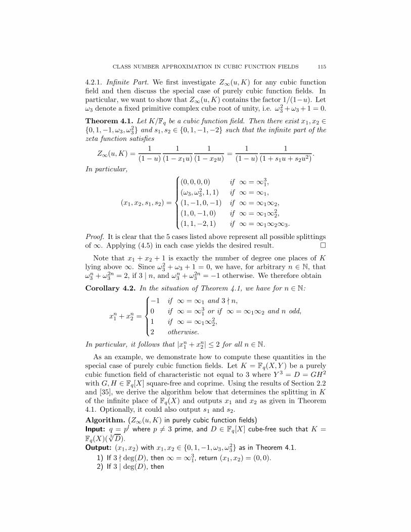
4.2.1. Infinite Part. We first investigate Z∞(u,K) for any cubic functionfield and then discuss the special case of purely cubic function fields. Inparticular, we want to show that Z∞(u,K) contains the factor 1/(1−u). Letω3 denote a fixed primitive complex cube root of unity, i.e. ω2
3 +ω3 +1 = 0.
Theorem 4.1. Let K/Fq be a cubic function field. Then there exist x1, x2 ∈{0, 1,−1, ω3, ω
23} and s1, s2 ∈ {0, 1,−1,−2} such that the infinite part of the
zeta function satisfies
Z∞(u,K) =1
(1 − u)
1
(1 − x1u)
1
(1 − x2u)=
1
(1 − u)
1
(1 + s1u+ s2u2).
In particular,
(x1, x2, s1, s2) =
(0, 0, 0, 0) if ∞ = ∞31,
(ω3, ω23 , 1, 1) if ∞ = ∞1,
(1,−1, 0,−1) if ∞ = ∞1∞2,
(1, 0,−1, 0) if ∞ = ∞1∞22,
(1, 1,−2, 1) if ∞ = ∞1∞2∞3.
Proof. It is clear that the 5 cases listed above represent all possible splittingsof ∞. Applying (4.5) in each case yields the desired result. �
Note that x1 + x2 + 1 is exactly the number of degree one places of Klying above ∞. Since ω2
3 + ω3 + 1 = 0, we have, for arbitrary n ∈ N, thatωn3 + ω2n
3 = 2, if 3 | n, and ωn3 + ω2n3 = −1 otherwise. We therefore obtain
Corollary 4.2. In the situation of Theorem 4.1, we have for n ∈ N:
xn1 + xn2 =
−1 if ∞ = ∞1 and 3 - n,
0 if ∞ = ∞31 or if ∞ = ∞1∞2 and n odd,
1 if ∞ = ∞1∞22,
2 otherwise.
In particular, it follows that |xn1 + xn2 | ≤ 2 for all n ∈ N.
As an example, we demonstrate how to compute these quantities in thespecial case of purely cubic function fields. Let K = Fq(X,Y ) be a purelycubic function field of characteristic not equal to 3 where Y 3 = D = GH2
with G,H ∈ Fq[X] square-free and coprime. Using the results of Section 2.2and [35], we derive the algorithm below that determines the splitting in Kof the infinite place of Fq(X) and outputs x1 and x2 as given in Theorem4.1. Optionally, it could also output s1 and s2.
Algorithm. (Z∞(u,K) in purely cubic function fields)Input: q = pl where p 6= 3 prime, and D ∈ Fq[X] cube-free such that K =
Fq(X)( 3√D).
Output: (x1, x2) with x1, x2 ∈ {0, 1,−1, ω3, ω23} as in Theorem 4.1.
1) If 3 - deg(D), then ∞ = ∞31, return (x1, x2) = (0, 0).
2) If 3 | deg(D), then
116 RENATE SCHEIDLER AND ANDREAS STEIN
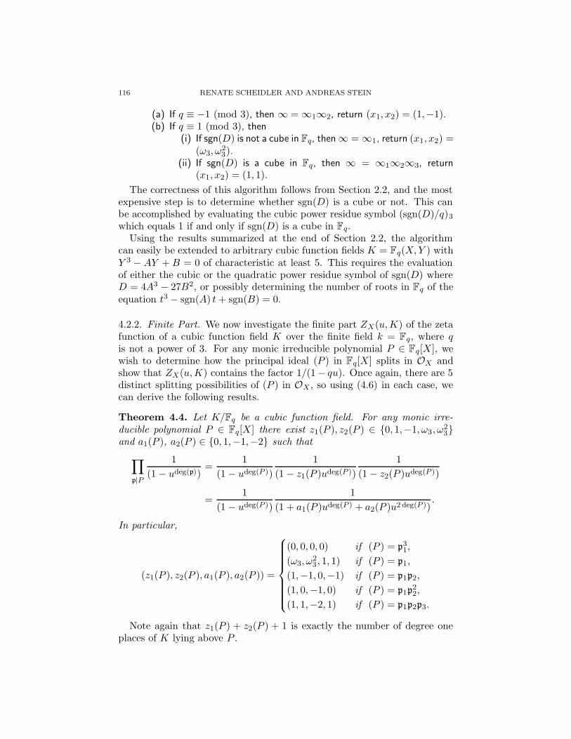
(a) If q ≡ −1 (mod 3), then ∞ = ∞1∞2, return (x1, x2) = (1,−1).(b) If q ≡ 1 (mod 3), then
(i) If sgn(D) is not a cube in Fq, then ∞ = ∞1, return (x1, x2) =(ω3, ω
23).
(ii) If sgn(D) is a cube in Fq, then ∞ = ∞1∞2∞3, return(x1, x2) = (1, 1).
The correctness of this algorithm follows from Section 2.2, and the mostexpensive step is to determine whether sgn(D) is a cube or not. This canbe accomplished by evaluating the cubic power residue symbol (sgn(D)/q)3
which equals 1 if and only if sgn(D) is a cube in Fq.Using the results summarized at the end of Section 2.2, the algorithm
can easily be extended to arbitrary cubic function fields K = Fq(X,Y ) withY 3 − AY + B = 0 of characteristic at least 5. This requires the evaluationof either the cubic or the quadratic power residue symbol of sgn(D) whereD = 4A3 − 27B2, or possibly determining the number of roots in Fq of theequation t3 − sgn(A) t+ sgn(B) = 0.
4.2.2. Finite Part. We now investigate the finite part ZX(u,K) of the zetafunction of a cubic function field K over the finite field k = Fq, where qis not a power of 3. For any monic irreducible polynomial P ∈ Fq[X], wewish to determine how the principal ideal (P ) in Fq[X] splits in OX andshow that ZX(u,K) contains the factor 1/(1 − qu). Once again, there are 5distinct splitting possibilities of (P ) in OX , so using (4.6) in each case, wecan derive the following results.
Theorem 4.4. Let K/Fq be a cubic function field. For any monic irre-ducible polynomial P ∈ Fq[X] there exist z1(P ), z2(P ) ∈ {0, 1,−1, ω3, ω
23}
and a1(P ), a2(P ) ∈ {0, 1,−1,−2} such that
∏
p|P
1
(1 − udeg(p))=
1
(1 − udeg(P ))
1
(1 − z1(P )udeg(P ))
1
(1 − z2(P )udeg(P ))
=1
(1 − udeg(P ))
1
(1 + a1(P )udeg(P ) + a2(P )u2 deg(P )).
In particular,
(z1(P ), z2(P ), a1(P ), a2(P )) =
(0, 0, 0, 0) if (P ) = p31,
(ω3, ω23 , 1, 1) if (P ) = p1,
(1,−1, 0,−1) if (P ) = p1p2,
(1, 0,−1, 0) if (P ) = p1p22,
(1, 1,−2, 1) if (P ) = p1p2p3.
Note again that z1(P ) + z2(P ) + 1 is exactly the number of degree oneplaces of K lying above P .
CLASS NUMBER APPROXIMATION IN CUBIC FUNCTION FIELDS 117
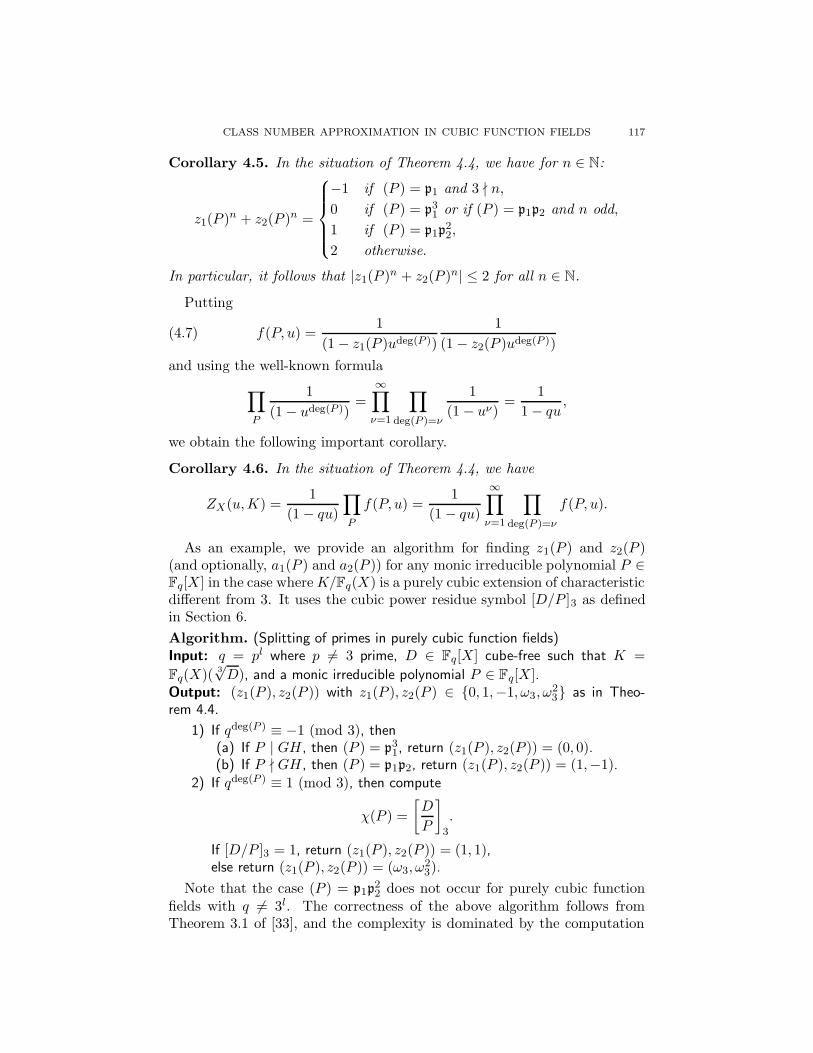
Corollary 4.5. In the situation of Theorem 4.4, we have for n ∈ N:
z1(P )n + z2(P )n =
−1 if (P ) = p1 and 3 - n,
0 if (P ) = p31 or if (P ) = p1p2 and n odd,
1 if (P ) = p1p22,
2 otherwise.
In particular, it follows that |z1(P )n + z2(P )n| ≤ 2 for all n ∈ N.
Putting
(4.7) f(P, u) =1
(1 − z1(P )udeg(P ))
1
(1 − z2(P )udeg(P ))
and using the well-known formula
∏
P
1
(1 − udeg(P ))=
∞∏
ν=1
∏
deg(P )=ν
1
(1 − uν)=
1
1 − qu,
we obtain the following important corollary.
Corollary 4.6. In the situation of Theorem 4.4, we have
ZX(u,K) =1
(1 − qu)
∏
P
f(P, u) =1
(1 − qu)
∞∏
ν=1
∏
deg(P )=ν
f(P, u).
As an example, we provide an algorithm for finding z1(P ) and z2(P )(and optionally, a1(P ) and a2(P )) for any monic irreducible polynomial P ∈Fq[X] in the case whereK/Fq(X) is a purely cubic extension of characteristicdifferent from 3. It uses the cubic power residue symbol [D/P ]3 as definedin Section 6.
Algorithm. (Splitting of primes in purely cubic function fields)Input: q = pl where p 6= 3 prime, D ∈ Fq[X] cube-free such that K =
Fq(X)( 3√D), and a monic irreducible polynomial P ∈ Fq[X].
Output: (z1(P ), z2(P )) with z1(P ), z2(P ) ∈ {0, 1,−1, ω3, ω23} as in Theo-
rem 4.4.
1) If qdeg(P ) ≡ −1 (mod 3), then(a) If P | GH, then (P ) = p3
1, return (z1(P ), z2(P )) = (0, 0).(b) If P - GH, then (P ) = p1p2, return (z1(P ), z2(P )) = (1,−1).
2) If qdeg(P ) ≡ 1 (mod 3), then compute
χ(P ) =
[
D
P
]
3
.
If [D/P ]3 = 1, return (z1(P ), z2(P )) = (1, 1),else return (z1(P ), z2(P )) = (ω3, ω
23).
Note that the case (P ) = p1p22 does not occur for purely cubic function
fields with q 6= 3l. The correctness of the above algorithm follows fromTheorem 3.1 of [33], and the complexity is dominated by the computation
118 RENATE SCHEIDLER AND ANDREAS STEIN
of gcd(D,P ) in the case where qdeg(P ) ≡ −1 (mod 3) and the evaluation of
[D/P ]3 in the case where qdeg(P ) ≡ 1 (mod 3). Algorithm 6.2 in Section 6shows that both scenarios yield essentially the same running time.
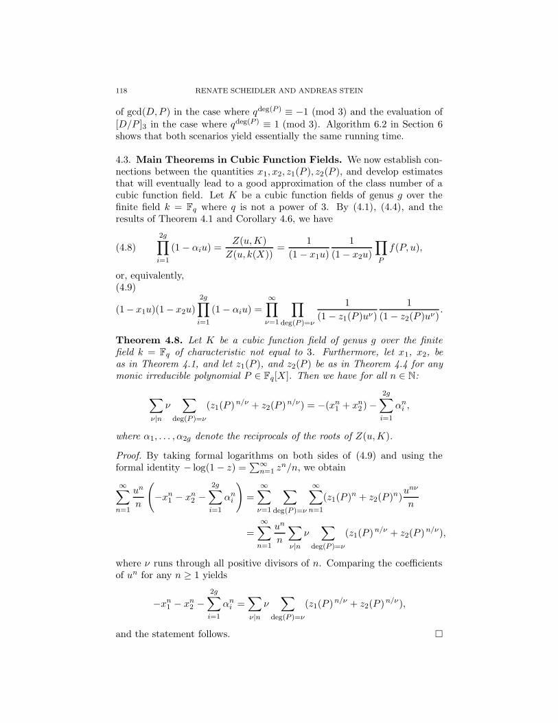
4.3. Main Theorems in Cubic Function Fields. We now establish con-nections between the quantities x1, x2, z1(P ), z2(P ), and develop estimatesthat will eventually lead to a good approximation of the class number of acubic function field. Let K be a cubic function fields of genus g over thefinite field k = Fq where q is not a power of 3. By (4.1), (4.4), and theresults of Theorem 4.1 and Corollary 4.6, we have
(4.8)
2g∏
i=1
(1 − αiu) =Z(u,K)
Z(u, k(X))=
1
(1 − x1u)
1
(1 − x2u)
∏
P
f(P, u),
or, equivalently,(4.9)
(1− x1u)(1 − x2u)
2g∏
i=1
(1 − αiu) =∞∏
ν=1
∏
deg(P )=ν
1
(1 − z1(P )uν)
1
(1 − z2(P )uν).
Theorem 4.8. Let K be a cubic function field of genus g over the finitefield k = Fq of characteristic not equal to 3. Furthermore, let x1, x2, beas in Theorem 4.1, and let z1(P ), and z2(P ) be as in Theorem 4.4 for anymonic irreducible polynomial P ∈ Fq[X]. Then we have for all n ∈ N:
∑
ν|n
ν∑
deg(P )=ν
(z1(P )n/ν + z2(P )n/ν) = −(xn1 + xn2 ) −2g∑
i=1
αni ,
where α1, . . . , α2g denote the reciprocals of the roots of Z(u,K).
Proof. By taking formal logarithms on both sides of (4.9) and using theformal identity − log(1 − z) =
∑∞n=1 z
n/n, we obtain
∞∑
n=1
un
n
(
−xn1 − xn2 −2g∑
i=1
αni
)
=
∞∑
ν=1
∑
deg(P )=ν
∞∑
n=1
(z1(P )n + z2(P )n)unν
n
=
∞∑
n=1
un
n
∑
ν|n
ν∑
deg(P )=ν
(z1(P )n/ν + z2(P )n/ν),
where ν runs through all positive divisors of n. Comparing the coefficientsof un for any n ≥ 1 yields
−xn1 − xn2 −2g∑
i=1
αni =∑
ν|n
ν∑
deg(P )=ν
(z1(P )n/ν + z2(P )n/ν),
and the statement follows. �
CLASS NUMBER APPROXIMATION IN CUBIC FUNCTION FIELDS 119
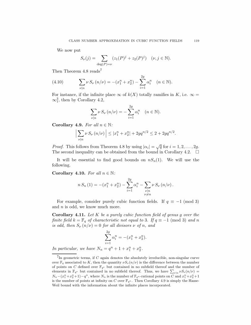
We now put
Sν(j) =∑
deg(P )=ν
(z1(P )j + z2(P )j) (ν, j ∈ N).
Then Theorem 4.8 reads7
(4.10)∑
ν|n
ν Sν (n/ν) = −(xn1 + xn2 ) −2g∑
i=1
αni (n ∈ N).
For instance, if the infinite place ∞ of k(X) totally ramifies in K, i.e. ∞ =∞3
1, then by Corollary 4.2,
∑
ν|n
ν Sν (n/ν) = −2g∑
i=1
αni (n ∈ N).
Corollary 4.9. For all n ∈ N:∣
∣
∣
∑
ν|n
ν Sν (n/ν)∣
∣
∣≤ |xn1 + xn2 | + 2gqn/2 ≤ 2 + 2gqn/2.
Proof. This follows from Theorem 4.8 by using |αi| =√q for i = 1, 2, . . . , 2g.
The second inequality can be obtained from the bound in Corollary 4.2. �
It will be essential to find good bounds on nSn(1). We will use thefollowing.
Corollary 4.10. For all n ∈ N:
nSn (1) = −(xn1 + xn2 ) −2g∑
i=1
αni −∑
ν|nν 6=n
ν Sν (n/ν) .
For example, consider purely cubic function fields. If q ≡ −1 (mod 3)and n is odd, we know much more.
Corollary 4.11. Let K be a purely cubic function field of genus g over thefinite field k = Fq of characteristic not equal to 3. If q ≡ −1 (mod 3) and nis odd, then Sν (n/ν) = 0 for all divisors ν of n, and
2g∑
i=1
αni = −(xn1 + xn2 ).
In particular, we have Nn = qn + 1 + xn1 + xn2 .
7In geometric terms, if C again denotes the absolutely irreducible, non-singular curveover Fq associated to K, then the quantity νSν(n/ν) is the difference between the numberof points on C defined over Fqν but contained in no subfield thereof and the number ofelements in Fqν but contained in no subfield thereof. Thus, we have
P
ν|n νSν(n/ν) =
Nn−(xn1 +xn
2 +1)−qn, where Nn is the number of Fqn-rational points on C and xn1 +xn
2 +1is the number of points at infinity on C over Fqn . Then Corollary 4.9 is simply the Hasse-Weil bound with the information about the infinite places incorporated.
120 RENATE SCHEIDLER AND ANDREAS STEIN
Proof. Let ν be a divisor of n. Since n is odd, ν and n/ν are odd. LetP ∈ Fq[X] be any monic irreducible polynomial of degree deg(P ) = ν. FromAlgorithm 4.7, we see that there are only two possible cases. If P | GH,then z1(P ) = z2(P ) = 0. If P - GH, then z1(P ) = 1 = −z2(P ). In bothcases, we have
z1(P )n/ν + z2(P )n/ν = 0.
Since P was arbitrary, Sν (n/ν) = 0 and therefore∑
ν|n
ν Sν (n/ν) = 0.
The result now follows from (4.10). �
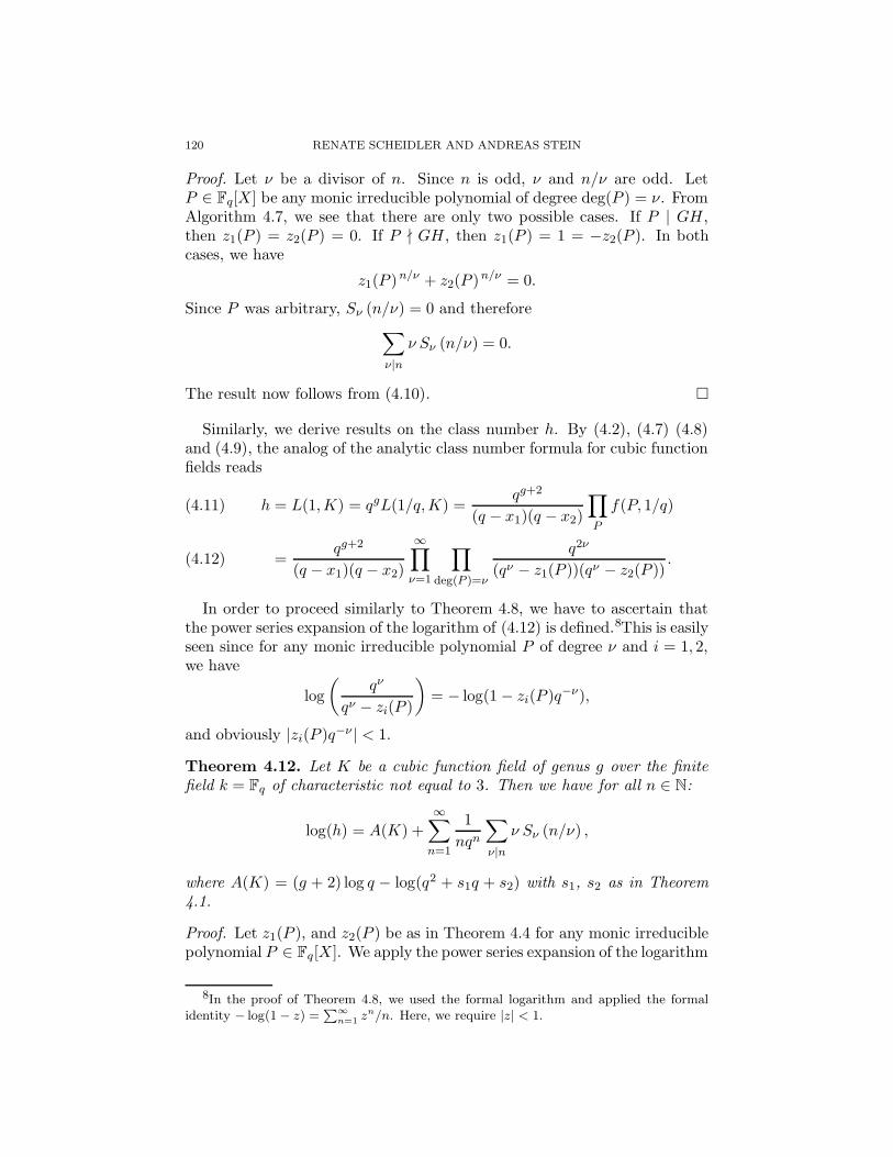
Similarly, we derive results on the class number h. By (4.2), (4.7) (4.8)and (4.9), the analog of the analytic class number formula for cubic functionfields reads
h = L(1,K) = qgL(1/q,K) =qg+2
(q − x1)(q − x2)
∏
P
f(P, 1/q)(4.11)
=qg+2
(q − x1)(q − x2)
∞∏
ν=1
∏
deg(P )=ν
q2ν
(qν − z1(P ))(qν − z2(P )).(4.12)
In order to proceed similarly to Theorem 4.8, we have to ascertain thatthe power series expansion of the logarithm of (4.12) is defined.8This is easilyseen since for any monic irreducible polynomial P of degree ν and i = 1, 2,we have
log
(
qν
qν − zi(P )
)
= − log(1 − zi(P )q−ν),
and obviously |zi(P )q−ν | < 1.
Theorem 4.12. Let K be a cubic function field of genus g over the finitefield k = Fq of characteristic not equal to 3. Then we have for all n ∈ N:
log(h) = A(K) +
∞∑
n=1
1
nqn
∑
ν|n
ν Sν (n/ν) ,
where A(K) = (g + 2) log q − log(q2 + s1q + s2) with s1, s2 as in Theorem4.1.
Proof. Let z1(P ), and z2(P ) be as in Theorem 4.4 for any monic irreduciblepolynomial P ∈ Fq[X]. We apply the power series expansion of the logarithm
8In the proof of Theorem 4.8, we used the formal logarithm and applied the formalidentity − log(1 − z) =
P∞n=1 zn/n. Here, we require |z| < 1.
CLASS NUMBER APPROXIMATION IN CUBIC FUNCTION FIELDS 121
to (4.12). As in the proof of Theorem 4.8, we obtain
log(h) = log
(
qg+2
(q − x1)(q − x2)
)
+∞∑
ν=1
∑
deg(P )=ν
∞∑
n=1
(z1(P )n + z2(P )n)1
nqnν
= A(K) +
∞∑
n=1
1
nqn
∑
ν|n
ν∑
deg(P )=ν
(z1(P )n/ν + z2(P )n/ν)
= A(K) +
∞∑
n=1
1
nqn
∑
ν|n
ν Sν (n/ν) ,
by definition of Sν (n/ν). Note that (q − x1)(q − x2) = q2 + s1q + s2. �
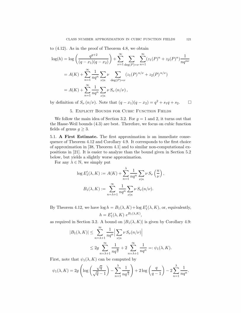
5. Explicit Bounds for Cubic Function Fields
We follow the main idea of Section 3.2. For g = 1 and 2, it turns out thatthe Hasse-Weil bounds (4.3) are best. Therefore, we focus on cubic functionfields of genus g ≥ 3.
5.1. A First Estimate. The first approximation is an immediate conse-quence of Theorem 4.12 and Corollary 4.9. It corresponds to the first choiceof approximation in [38, Theorem 4.1] and to similar non-computational ex-positions in [21]. It is easier to analyze than the bound given in Section 5.2below, but yields a slightly worse approximation.
For any λ ∈ N, we simply put
logE′1(λ,K) := A(K) +
λ∑
n=1
1
nqn
∑
ν|n
ν Sν
(n
ν
)
,
B1(λ,K) :=
∞∑
n=λ+1
1
nqn
∑
ν|n
ν Sν(n/ν).
By Theorem 4.12, we have log h = B1(λ,K)+ logE ′1(λ,K), or, equivalently,
h = E′1(λ,K) eB1(λ,K),
as required in Section 3.2. A bound on |B1(λ,K)| is given by Corollary 4.9:
|B1(λ,K)| ≤∞∑
n=λ+1
1
nqn
∣
∣
∣
∑
ν|n
ν Sν(n/ν)∣
∣
∣
≤ 2g
∞∑
n=λ+1
1
nqn2
+ 2
∞∑
n=λ+1
1
nqn=: ψ1(λ,K).
First, note that ψ1(λ,K) can be computed by
ψ1(λ,K) = 2g
(
log
( √q
√q − 1
)
−λ∑
n=1
1
nqn2
)
+ 2 log
(
q
q − 1
)
− 2
λ∑
n=1
1
nqn.
122 RENATE SCHEIDLER AND ANDREAS STEIN
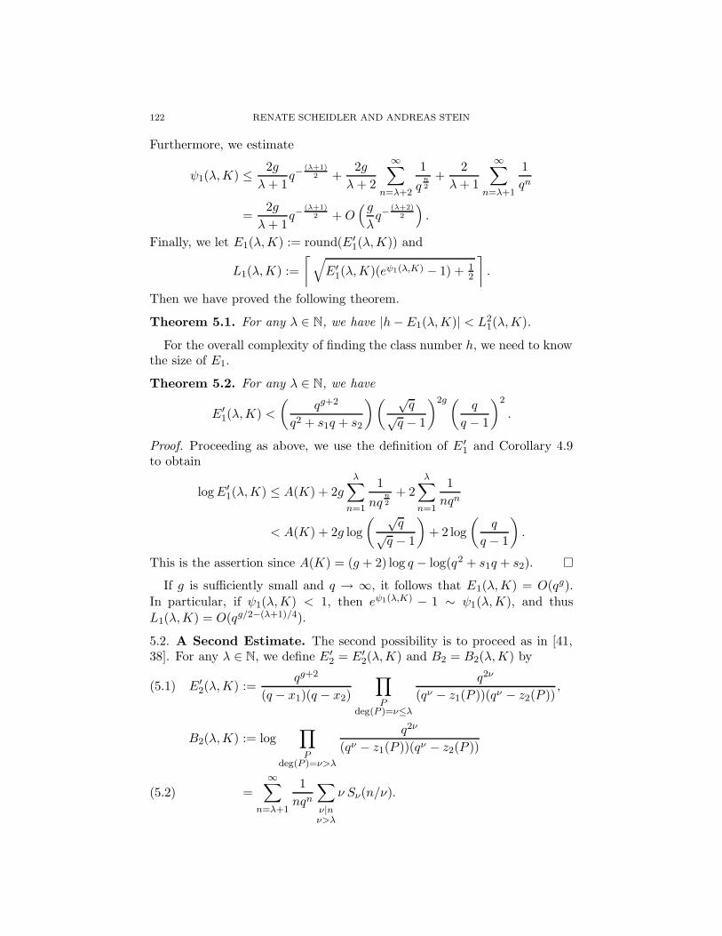
Furthermore, we estimate
ψ1(λ,K) ≤ 2g
λ+ 1q−
(λ+1)2 +
2g
λ+ 2
∞∑
n=λ+2
1
qn2
+2
λ+ 1
∞∑
n=λ+1
1
qn
=2g
λ+ 1q−
(λ+1)2 +O
( g
λq−
(λ+2)2
)
.
Finally, we let E1(λ,K) := round(E ′1(λ,K)) and
L1(λ,K) :=
⌈
√
E′1(λ,K)(eψ1(λ,K) − 1) + 1
2
⌉
.
Then we have proved the following theorem.
Theorem 5.1. For any λ ∈ N, we have |h−E1(λ,K)| < L21(λ,K).
For the overall complexity of finding the class number h, we need to knowthe size of E1.
Theorem 5.2. For any λ ∈ N, we have
E′1(λ,K) <
(
qg+2
q2 + s1q + s2
)( √q
√q − 1
)2g ( q
q − 1
)2
.
Proof. Proceeding as above, we use the definition of E ′1 and Corollary 4.9
to obtain
logE′1(λ,K) ≤ A(K) + 2g
λ∑
n=1
1
nqn2
+ 2
λ∑
n=1
1
nqn
< A(K) + 2g log
( √q
√q − 1
)
+ 2 log
(
q
q − 1
)
.
This is the assertion since A(K) = (g + 2) log q − log(q2 + s1q + s2). �
If g is sufficiently small and q → ∞, it follows that E1(λ,K) = O(qg).
In particular, if ψ1(λ,K) < 1, then eψ1(λ,K) − 1 ∼ ψ1(λ,K), and thus
L1(λ,K) = O(qg/2−(λ+1)/4).
5.2. A Second Estimate. The second possibility is to proceed as in [41,38]. For any λ ∈ N, we define E ′
2 = E′2(λ,K) and B2 = B2(λ,K) by
E′2(λ,K) :=
qg+2
(q − x1)(q − x2)
∏
Pdeg(P )=ν≤λ
q2ν
(qν − z1(P ))(qν − z2(P )),(5.1)
B2(λ,K) := log∏
Pdeg(P )=ν>λ
q2ν
(qν − z1(P ))(qν − z2(P ))
=
∞∑
n=λ+1
1
nqn
∑
ν|nν>λ
ν Sν(n/ν).(5.2)
CLASS NUMBER APPROXIMATION IN CUBIC FUNCTION FIELDS 123
Note that E ′2(λ,K) contains more information about h than E ′
1(λ,K), sinceall computable information for polynomials up to degree λ is included inE′
2(λ,K). For hyperelliptic curves, this estimate yielded faster computa-tional results than the first estimate. We have
logE′2(λ,K) = A(K) +
λ∑
n=1
1
nqn
∑
ν|n
ν Sν(n/ν) +
∞∑
n=λ+1
1
nqn
∑
ν|nν≤λ
ν Sν(n/ν),
and by (4.11) and Theorem 4.12, we have
h = E′2(λ,K) eB2(λ,K).
If we put E2(λ,K) := round(E ′2(λ,K)), then E2(λ,K) is an approximation
of h. As pointed out in Section 3.2, we need to find a sharp upper boundon |B2(λ,K)|. From (5.2), we see that
(5.3) B2(λ,K) =Sλ+1(1)
qλ+1+
∞∑
n=λ+2
1
nqn
∑
ν|nν>λ
ν Sν(n/ν).
The dominant term of B2(λ,K) is Sλ+1(1)/qλ+1. In order to find sharp
upper bounds on |B2(λ,K)|, we need to investigate Sν(j), particularly Sν(1).We denote by Iν the number of monic prime polynomials of degree ν.
Then νIν is the number of elements in Fqν but contained in no subfieldthereof, and it is well-known that
∑
ν|n νIν = qn for all n ∈ N. Also, Mobius
inversion9 implies that
(5.4) nIn =∑
ν|n
µ(n/ν)qν = qn +∑
ν|nν 6=n
µ(n/ν)qν (n ∈ N) .
Lemma 5.3. For ν, j, l ∈ N, we have
a) Sν(j + 6l) = Sν(j).
b) If 3 - j, then Sν(j) =
{
Sν(1) if j odd,
Sν(2) if j even.
c) |Sν(j)| ≤ 2Iν .
Proof. It is easy to see that zi(P )j+6l = z1(P ) for i = 1, 2, and if 3 - j,then z1(P )j + z2(P )j = z1(P ) + z2(P ) if j is odd, and z1(P )j + z2(P )j =z1(P )2 + z2(P )2 if j is even. Parts a) and b) now follow from the definitionof Sν(j). Furthermore, |z1(P )j + z2(P )j | ≤ 2 by Corollary 4.5, so Sν(j) ≤∑
deg(P )=ν 2 = 2Iν . �
Since z1(P )6 = z2(P )6 = 1 if the ideal (P ) is unramified, it is clear thatSν(6) and 2Iν agree except for the irreducible polynomials for which the
9If f is an arithmetic function and F (n) =P
ν|n f(ν) for n ∈ N, then f(n) =P
ν|n µ(n/ν)F (ν) where µ denotes the Mobius function.
124 RENATE SCHEIDLER AND ANDREAS STEIN
ideal (P ) ramifies. Next, we want to bound nSn(1). By Corollary 4.10, weneed to bound
∑
ν|nν 6=n
ν Sν (n/ν).
Lemma 5.4. For n ∈ N,
n|Sn(1)| ≤ 2gqn2 +2+
2q
(q − 1)
(qn2 − 1) if n even
(qn3 − 1) if n odd
< (2g+2)qn2
q
(q − 1).
Proof. Lemma 5.3 c) and (5.4) yield∣
∣
∣
∑
ν|nν 6=n
ν Sν (n/ν)∣
∣
∣≤∑
ν|nν 6=n
ν|Sν (n/ν) | ≤ 2∑
ν|nν 6=n
νIν = 2(
∑
ν|n
νIν − nIn
)
= 2(qn − nIn) = −2∑
ν|nν 6=n
µ(n/ν)qν ≤ 2∑
ν|nν 6=n
qν
≤
2
n/2∑
ν=1
qν ≤ 2(qn2 − 1)q/(q − 1) if n even,
2bn/3c∑
ν=1qν ≤ 2(q
n3 − 1)q/(q − 1) if n odd.
By Corollary 4.10, we get
n|Sn(1)| ≤ |xn1 + xn2 | + 2gqn2 +
∣
∣
∣
∑
ν|nν 6=n
ν Sν (n/ν)∣
∣
∣
since |αi| =√q for i = 1, 2, . . . , 2g. The first estimate then follows from the
above and Corollary 4.2. For the second inequality, we note that
2 + 2gqn2 + 2
(qn2 − 1)q
(q − 1)< 2 + (2g + 2)q
n2
q
(q − 1)− 2q
(q − 1).
�
We will use the first bound of the lemma in implementations and thesecond bound for estimating the tail of the truncated Euler product. Alsonotice that another (in general less sharp) bound would be n|Sn(1)| < (2g+
4)qn2 .
Example 5.5. For small genus, the bound in Lemma 5.4 is relatively sharp.For instance, let K be a purely cubic function field K = Fq(X,Y ) of char-acteristic different from 3 where Y 3 = D, and D ∈ Fq[X] is irreduciblewith deg(D) > 1. Then there are no ramified prime polynomials in Fq[x]of degree 1. Furthermore, if we assume that q ≡ 1 (mod 3), then all monicprime polynomials P ∈ Fq[x] of degree 1 are either inert or totally split (be-cause K/Fq(x) is a Galois extension), so z1(P )3 = z2(P )3 = 1, and hence
CLASS NUMBER APPROXIMATION IN CUBIC FUNCTION FIELDS 125
S1(3) = 2I1 = 2q. By Corollary 4.10,
3S3(1) = −x31 − x3
2 −2g∑
i=1
α3i − S1(3) = −2 −
2g∑
i=1
α3i − 2q .
On the other hand, the bound of Lemma 5.4 yields
3|S3(1)| ≤ 2 + 2gq32 + |S1(3)| ≤ 2 + 2gq
32 + 2q.
In this situation, this is the best possible bound, unless we have more infor-mation about |∑2g
i=1 α3i |.
Lemma 5.6. For λ, n ∈ N with λ < n, we have∣
∣
∣
∑
ν|nν>λ
ν Sν(n/ν)∣
∣
∣< (2g + 4)
q
(q − 1)q
n2 .
Proof. Note that∑
ν|nν>λ
ν Sν(n/ν) = nSn(1) +∑
ν|nλ<ν<n
ν Sν(n/ν).
We can use the result of Lemma 5.4 and proceed as in the proof of thatLemma to obtain
∣
∣
∣
∑
ν|nν>λ
ν Sν(n/ν)∣
∣
∣≤ 2 + 2gq
n2 + 4
(qn2 − 1)q
(q − 1)< (2g + 4)q
n2
q
(q − 1).
�
We use the previous lemma to bound the second summand in (5.3).
Lemma 5.7. For λ ∈ N, we have
∣
∣
∣
∞∑
n=λ+2
1
nqn
∑
ν|nν>λ
ν Sν(n/ν)∣
∣
∣<
(2g + 4)
(λ+ 2)
√q
(√q − 1)
q
(q − 1)q−
λ+22 .
Proof. We use Lemma 5.6 to obtain
∣
∣
∣
∞∑
n=λ+2
1
nqn
∑
ν|nν>λ
ν Sν(n/ν)∣
∣
∣≤ (2g + 4)
q
(q − 1)
∞∑
n=λ+2
1
nqn2
<(2g + 4)
(λ+ 2)
q
(q − 1)
∞∑
n=λ+2
1
qn2
≤ (2g + 4)
(λ+ 2)
q
(q − 1)
√q
(√q − 1)
q−λ+22 .
�
126 RENATE SCHEIDLER AND ANDREAS STEIN
We are now able to define an upper bound on B2(λ,K). For λ ∈ N, wedefine
ψ2(λ,K) =2g
λ+ 1q−
λ+12 +
(2g + 4)
(λ+ 2)
√q
(√q − 1)
q
(q − 1)q−
λ+22 +
2
λ+ 1q−(λ+1)
+2
(λ+ 1)
q
(q − 1)q−(λ+1)
(qλ+1
2 − 1) if λ odd,
(qλ+1
3 − 1) if λ even.
By the previous lemmas and (5.3), we derive that |B2(λ,K)| < ψ2(λ,K).Thus, ψ2(λ,K) is the required bound on |B2(λ,K)|. Again, we put
E2(λ,K) := round(E ′2(λ,K)),
L2(λ,K) :=
⌈
√
E′2(λ,K)(eψ2(λ,K) − 1) + 1
2
⌉
.
Theorem 5.8. For any λ ∈ N, we have |h−E2(λ,K)| < L22(λ,K).
Theorem 5.9. For any λ ∈ N, we have
E′2(λ,K) ≤
(
qg+2
q2 + s1q + s2
)( √q
√q − 1
)2g ( q
q − 1
)2
eψ2(λ,K).
Proof. By (5.1), we have
logE′2(λ,K) = A(K) +
∞∑
n=1
1
nqn
∑
ν|n
ν Sν(n/ν) −B2(λ,K).
From the proof of Theorem 5.2, it follows that
| logE′2(λ,K)| ≤ A(K) + 2g log
( √q
√q − 1
)
+ 2 log
(
q
q − 1
)
+ ψ2(λ,K).
This is the statement. �
For small g and large q, we conclude that E2(λ,K) = O(qg). If ψ2(λ,K) <
1, then we have L2(λ,K) = O(qg/2−(λ+1)/4) as q → ∞.
5.3. Complexity Analysis and Optimization. The complexity analysisis analogous to the one in Section 5.1 of [38]. We follow the idea of Sections3.1 and 3.2. If g ≤ 2, the Hasse-Weil bound (4.3) is best. More precisely, ifg = 1 or 2 then the total running time for computing an approximation of h,and subsequently finding h, is O(q 1/4) and O(q 3/4), respectively. For g ≥ 3,we put E = E ′
2(λ,K) and L = L2(λ,K). Since determining E requiresthe computation of O(qλ) values z1(P ), z2(P ), the estimate on L yields acomplexity of max{O(qλ), O(qg/2−(λ+1)/4)} for finding h. Thus, the optimalchoice for λ is
λ =
{
b(2g − 1)/5c if g ≡ 2 (mod 5),
round((2g − 1)/5) otherwise.(5.5)
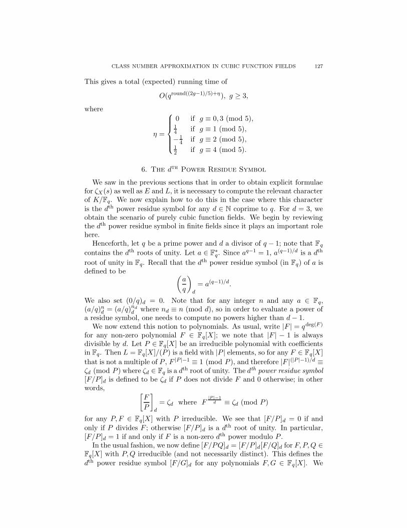
CLASS NUMBER APPROXIMATION IN CUBIC FUNCTION FIELDS 127
This gives a total (expected) running time of
O(qround((2g−1)/5)+η ), g ≥ 3,
where
η =
0 if g ≡ 0, 3 (mod 5),14 if g ≡ 1 (mod 5),
−14 if g ≡ 2 (mod 5),
12 if g ≡ 4 (mod 5).
6. The dth Power Residue Symbol
We saw in the previous sections that in order to obtain explicit formulaefor ζX(s) as well as E and L, it is necessary to compute the relevant characterof K/Fq. We now explain how to do this in the case where this character
is the dth power residue symbol for any d ∈ N coprime to q. For d = 3, weobtain the scenario of purely cubic function fields. We begin by reviewingthe dth power residue symbol in finite fields since it plays an important rolehere.
Henceforth, let q be a prime power and d a divisor of q − 1; note that Fqcontains the dth roots of unity. Let a ∈ F∗
q. Since aq−1 = 1, a(q−1)/d is a dth
root of unity in Fq. Recall that the dth power residue symbol (in Fq) of a isdefined to be
(
a
q
)
d
= a(q−1)/d.
We also set (0/q)d = 0. Note that for any integer n and any a ∈ Fq,(a/q)nd = (a/q)nd
d where nd ≡ n (mod d), so in order to evaluate a power ofa residue symbol, one needs to compute no powers higher than d− 1.
We now extend this notion to polynomials. As usual, write |F | = qdeg(F )
for any non-zero polynomial F ∈ Fq[X]; we note that |F | − 1 is alwaysdivisible by d. Let P ∈ Fq[X] be an irreducible polynomial with coefficientsin Fq. Then L = Fq[X]/(P ) is a field with |P | elements, so for any F ∈ Fq[X]
that is not a multiple of P , F |P |−1 ≡ 1 (mod P ), and therefore |F |(|P |−1)/d ≡ζd (mod P ) where ζd ∈ Fq is a dth root of unity. The dth power residue symbol[F/P ]d is defined to be ζd if P does not divide F and 0 otherwise; in otherwords,
[
F
P
]
d
= ζd where F|P |−1
d ≡ ζd (mod P )
for any P, F ∈ Fq[X] with P irreducible. We see that [F/P ]d = 0 if and
only if P divides F ; otherwise [F/P ]d is a dth root of unity. In particular,[F/P ]d = 1 if and only if F is a non-zero dth power modulo P .
In the usual fashion, we now define [F/PQ]d = [F/P ]d[F/Q]d for F, P,Q ∈Fq[X] with P,Q irreducible (and not necessarily distinct). This defines the
dth power residue symbol [F/G]d for any polynomials F,G ∈ Fq[X]. We
128 RENATE SCHEIDLER AND ANDREAS STEIN
summarize some properties that can be found in Propositions 3.2 and 3.4 aswell as Theorem 3.5, pp. 24-27, of [32].
Lemma 6.1. Let F, F1, F2, G ∈ Fq[X] and a ∈ Fq. Set f ≡ deg(F ) (mod d)and g ≡ deg(G) (mod d). Then the following properties hold:
1. If F1 ≡ F2 (mod G), then
[
F1
G
]
d
=
[
F2
G
]
d
.
2.
[
F1F2
G
]
d
=
[
F1
G
]
d
[
F2
G
]
d
.
3.
[
F
G1G2
]
d
=
[
F
G1
]
d
[
F
G2
]
d
.
4.
[
F
G
]
d
= 0 if and only if F and G are not coprime.
5.[ a
G
]
d=
(
a
q
)g
d
.
6.
[
F
G
]
d
=
(−1
q
)fg
d
(
sgn(F )
q
)g
d
(
sgn(G)
q
)−f
d
[
G
F
]
d
if F and G are co-
prime.
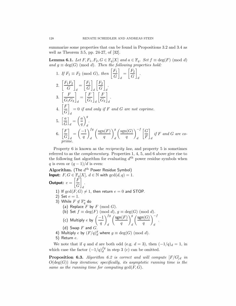
Property 6 is known as the reciprocity law, and property 5 is sometimesreferred to as the complementary. Properties 1, 4, 5, and 6 above give rise tothe following fast algorithm for evaluating dth power residue symbols whenq is even or (q − 1)/d is even:
Algorithm. (The dth Power Residue Symbol)Input: F,G ∈ Fq[X], d ∈ N with gcd(d, q) = 1.
Output: e =
[
F
G
]
d
.
1) If gcd(F,G) 6= 1, then return e = 0 and STOP.2) Set e = 1.3) While F 6∈ F∗
q do(a) Replace F by F (mod G).(b) Set f ≡ deg(F ) (mod d), g ≡ deg(G) (mod d).
(c) Multiply e by
(−1
q
)fg
d
(
sgn(F )
q
)g
d
(
sgn(G)
q
)−f
d
.
(d) Swap F and G.4) Multiply e by (F/q)gd where g ≡ deg(G) (mod d).5) Return e.
We note that if q and d are both odd (e.g. d = 3), then (−1/q)d = 1, in
which case the factor (−1/q)fgd in step 3 (c) can be omitted.
Proposition 6.3. Algorithm 6.2 is correct and will compute [F/G]d inO(deg(G)) loop iterations; specifically, its asymptotic running time is thesame as the running time for computing gcd(F,G).
CLASS NUMBER APPROXIMATION IN CUBIC FUNCTION FIELDS 129
Proof. Step 1 certainly returns the correct result by property 4. So supposethat F and G are coprime. Steps (a) and (d) of the while loop in step 3constitute simply the Euclidean Algorithm for computing gcd(F,G), startingwith dividing F by G. So the while loop is executed O(deg(G)) times andterminates with a remainder F that is a constant, since gcd(F,G) = 1.
Now step 3 (a) does not change the value of [F/G]d by property 1. Thereciprocity law (property 6) shows that the value of e is correctly modifiedin each iteration of the while loop. After the loop, F ∈ F∗
q, so by property 5,
[F/G]d is obtained by multiplying the current value of e by [F/G]d = (F/q)gdwith g ≡ deg(G) (mod d). �
7. Open Problems and Future Research
7.1. Cubic Function Fields. The formulae for E and L given in Section5 are still valid when there are more than two places at infinity. However,in this setting, it is not obvious how to use the baby step giant step orPollard kangaroo methods to search for h in the interval ]E − L2, E + L2[.The case where there is only one place at infinity, i.e. O∗
X = F∗q, simply
requires searching in a group; that is, searching on reduced (distinguished)representatives in the ideal class group of K/k(X). When there are twoinfinite places, i.e. K/k(X) has unit rank 1, the infrastructure as describedin [33] can be utilized for the search. But for higher unit rank, it is as yetunclear how to extend these techniques; this question definitely warrantsfurther study.
The analysis of purely cubic function fields of characteristic different from3 seems to carry over with few changes to the case of arbitrary cubic functionfields; an initial investigation was already done in [34] and includes an ex-plicit description of the splitting at infinity. The next step is to find a simplecharacterization of the splitting of the finite places (work in progress), andto extend the arithmetic and the investigation of the infrastructure given in[33] as well as the algorithms given in this paper from the purely cubic caseto the general setting.
We also mention that cubic function fields of characteristic 3 have notbeen researched at all. Their behavior is very different from that of theircounterparts of characteristic different from 3. Examples of such differencesinclude the possibility of wild ramification, and of course there is no analogto the purely cubic scenario; instead, certain cubic curves give rise to Artin-Schreier extensions in this case.
7.2. Function Fields of Higher Degree. Contrary to the situation ofalgebraic number fields, it is possible to construct function field extensionsof a given unit rank and arbitrary degree, since there is much more flexibilityfor the splitting at infinity. Number fields have eifi = 1 for real embeddingsand eifi = 2 for complex embeddings, whilst there is no such restriction onthe value of eifi in a function field. For example, the only number fields ofunit rank 0 are imaginary quadratic fields, whereas any function field with
130 RENATE SCHEIDLER AND ANDREAS STEIN
only one (totally inert or ramified) place at infinity has unit rank 0; thefamily of superelliptic function fields K = Fq(X,Y ) with Y n = D(X) andgcd(q, n) = gcd(deg(D), n) = 1 studied in [16] represent such examples.
There is a wealth of open problems pertaining to the arithmetic of ideals inboth algebraic number fields and algebraic function fields. Two approachesto this topic are prevalent. General purpose methods are applicable to anyextension, but they tend to be inefficient. In order to obtain efficiency,one may need to sacrifice generality and focus instead on special purposetechniques. This has already shown to be very successful in the quadraticand cubic scenarios of both number fields and function fields. No othernumber fields have been studied in any detail, with the exception of quarticfields which were investigated in a series of papers by Buchmann et al.[5, 6, 10, 12, 8, 7, 9]. In addition, a more general treatment of number fieldsof unit rank 1 (which always exhibit an infrastructure) can be found in [11].It is worthwhile to explore these ideas for their applicability to functionfields. A description of how the analytic class number can be used to findthe ideal class number of any number field was given in [11] and has inspiredsome of the ideas in this article.
8. Acknowledgements
The authors wish to thank an anonymous referee for carefully proof-reading the paper and making valuable suggestions. Furthermore, our thanksgo to Eric Landquist for suggesting improvements and useful changes to Sec-tion 4.
References
1. L. M. Adleman and M.-D. Huang, Counting rational points on curves and Abelian
varieties over finite fields, Algorithmic Number Theory ANTS-II (Berlin (Germany)),Lect. Notes Comput. Sci., vol. 1122, Springer-Verlag, 1996, pp. 1–16.
2. , Counting points on curves and Abelian varieties over finite fields, J. SymbolicComput. 32 (2001), 171–189.
3. M. Bauer, The arithmetic of certain cubic function fields, Math. Comp. 73 (2004),387–413.
4. M. Bauer, E. Teske, and A. Weng, Point counting on Picard curves in large charac-
teristic, Math. Comp. 74 (2005), 1983–2005.5. J. A. Buchmann, The computation of the fundamental unit of totally complex quartic
orders, Math. Comp. 48 (1987), 39–54.6. , On the computation of units and class numbers by a generalization of La-
grange’s algorithm, J. Number Theory 26 (1987), 8–30.7. J. A. Buchmann, D. Ford, and M. Pohst, Enumeration of quartic fields of small
discriminant, Math. Comp. 61 (1993), 873–879.8. J. A. Buchmann, M. Pohst, and J. Graf von Schmettow, On the computation of unit
groups and class groups of totally real quartic fields, Math. Comp. 53 (1989), 387–397.9. , On unit groups and class groups of quartic fields of signature (2, 1), Math.
Comp. 62 (1994), 387–390.10. J. A. Buchmann and H. C. Williams, On principal ideal testing in totally complex
quartic fields and the determination of certain cyclotomic constants, Math. Comp. 48
(1987), 55–66.
CLASS NUMBER APPROXIMATION IN CUBIC FUNCTION FIELDS 131
11. , On the computation of the class number of an algebraic number field, Math.Comp. 53 (1988), 679–688.
12. , On the infrastructure of the principal ideal class of an algebraic number field
of unit rank one, Math. Comp. 50 (1988), 569–579.13. W. Castryck, J. Denef, and F. Vercauteren, Computing zeta functions of nondegener-
ate curves, Internat. Math. Research Papers Article ID 72017 (2006), 1–57.14. J. Denef and F. Vercauteren, An extension of Kedlaya’s algorithm to Artin-Schreier
curves in characteristic 2, Algorithmic Number Theory ANTS-V (Berlin (Germany)),Lect. Notes Comput. Sci., vol. 2369, Springer-Verlag, 2002, pp. 308–323.
15. , Counting points on Cab curves using Monsky-Washnitzer cohomology, FiniteFields Appl. 12 (2006), 78–102.
16. S. D. Galbraith, S. Paulus, and N. P. Smart, Arithmetic on superelliptic curves, Math.Comp. 71 (2002), 393–405.
17. P. Gaudry and M. Gurel, An extension of Kedlaya’s point-counting algorithm to su-
perelliptic curves, Advances in Cryptology – ASIACRYPT 2001 (Berlin (Germany)),Lect. Notes Comput. Sci., vol. 2248, Springer-Verlag, 2001, pp. 480–494.
18. , Counting points in medium characteristic using Kedlaya’s algorithm, Exp.Math. 12 (2003), 395–402.
19. P. Gaudry and R. Harley, Counting points on hyperelliptic curves over finite fields,Algorithmic Number Theory ANTS-IV (Berlin (Germany)), Lect. Notes Comput. Sci.,vol. 1838, Springer-Verlag, 2000, pp. 313–332.
20. P. Gaudry and E. Schost, Construction of secure random curves of genus 2 over
prime fields, Advances in Cryptology – Eurocrypt 2004 (Berlin (Germany)), Lect.Notes Comput. Sci., vol. 3027, Springer-Verlag, 2004, pp. 239–256.
21. F. Hess, Zur divisorklassengruppenberechnung in globalen funktionenkorpern, Ph.D.thesis, Technische Universitat Berlin, Berlin (Germany), 1999.
22. M.-D. Huang and D. Ierardi, Counting points on curves over finite fields, J. Symb.Comput. 25 (1998), 1–21.
23. K. S. Kedlaya, Counting points on hyperelliptic curves using Monsky-Washnitzer co-
homology, J. Ramanujan Math. Soc. 16 (2001), 323–338.24. , Errata for “Counting points on hyperelliptic curves using Monsky-Washnitzer
cohomology”, J. Ramanujan Math. Soc. 18 (2003), 417–418.25. , Computing zeta functions via p-adic cohomology, Algorithmic Number Theory
ANTS-VI (Berlin (Germany)), Lect. Notes Comput. Sci., vol. 3076, Springer-Verlag,2004, pp. 1–17.
26. A. G. B. Lauder and D. Wan, Computing zeta functions of Artin-Schreier curves over
finite fields., LMS J. Comput. Math. 5 (2002), 34–55.27. , Computing zeta functions of Artin-Schreier curves over finite fields. ii, J.
Complexity 20 (2004), 331–349.28. A. G. B. Lauer, Computing zeta functions of Kummer curves via multiplicative char-
acters, Found. Comput. Math. 3 (2003), 273–295.29. Y. Lee, R. Scheidler, and C. Yarrish, Computation of the fundamental units and the
regulator of a cyclic cubic function field, Exp. Math. 12 (2003), 211–225.30. J. Pila, Frobenius maps of abelian varieties and finding roots of unity in finite fields,
Math. Comp. 55 (1990), 745–763.31. , Counting points on curves over families in polynomial time, eprint
arXiv:math/0504570 (2005).32. M. Rosen, Number theory in function fields, Springer-Verlag, Berlin (Germany), 2002.33. R. Scheidler, Ideal arithmetic and infrastructure in purely cubic function fields, J.
Theor. Nombr. Bordeaux 13 (2001), 609–631.34. , Algorithmic aspects of cubic function fields, Algorithmic Number Theory
ANTS-VI (Berlin (Germany)), Lect. Notes Comp. Sci., vol. 3976, Springer-Verlag,2004, pp. 395–410.
132 RENATE SCHEIDLER AND ANDREAS STEIN
35. R. Scheidler and A. Stein, Voronoi’s algorithm in purely cubic congruence function
fields of unit rank 1, Math. Comp. 69 (2000), 1245–1266.36. F. K. Schmidt, Analytische Zahlentheorie in Korpern der Charakteristik p, Math.
Zeitschr. 33 (1931), 1–32.37. R. Schoof, Counting points on elliptic curves over finite fields, J. Theor. Nombres
Bordeaux 7 (1995), 219–254.38. A. Stein and E. Teske, Explicit bounds and heuristics on class numbers in hyperelliptic
function fields, Math. Comp. 71 (2002), 837–861.39. , The parallelized Pollard kangaroo method in real quadratic function fields,
Math. Comp. 71 (2002), 793–814.40. , Optimized baby step-giant step methods, J. Ramanujan Math. Soc. 20 (2005),
27–58.41. A. Stein and H. C. Williams, Some methods for evaluating the regulator of a real
quadratic function field, Exper. Math. 8 (1999), 119–133.42. H. Stichtenoth, Algebraic function fields and codes, Springer-Verlag, Berlin (Ger-
many), 1993.
Department of Mathematics and Statistics, University of Calgary,
2500 University Drive NW, Calgary, Alberta T2N 1N4, Canada
E-mail address: [email protected]
Department of Mathematics, University of Wyoming,
P.O. Box 3036, 1000 E. University Avenue, Laramie, Wyoming 82071-3036, USA
E-mail address: [email protected]