CIS 467/602-01: Data Visualization

CIS 467, Spring 2015

CIS 467/602-01: Data Visualization

Vector Field Visualization

Dr. David Koop

Fields

2CIS 467, Spring 2015

Tables Networks & Trees

Fields Geometry Clusters, Sets, Lists

Items

Attributes

Items (nodes)

Links

Attributes

Grids

Positions

Attributes

Items

Positions

Items

Fields and Grids• Fields: values come from a continuous domain, infinitely many

values - Sampled at certain positions to approximate the entire domain - Positions are often aligned in grids

• Geometry: the spatial positions of the data (points) • Topology: how the points are connected (cells)


Grids (Meshes)• Meshes combine positional information (geometry) with

topological information (connectivity).

• Mesh type can differ substantial depending in the way mesh cells are formed.

From Weiskopf, Machiraju, Möller© Weiskopf/Machiraju/Möller

Data Structures

• Grid types– Grids differ substantially in the cells (basic

building blocks) they are constructed from and in the way the topological information is given

scattered uniform rectilinear structured unstructured[© Weiskopf/Machiraju/Möller]

Fields in Visualization


Scalar Fields Vector Fields Tensor Fields

Each point in space has an associated...

Vector Fields

s0

2

4�00 �01 �02

�10 �11 �12

�20 �21 �22

3

5

2

4v0

v1

v2

3

5



Scalar Fields Vector Fields Tensor Fields(Order-1 Tensor Fields)(Order-0 Tensor Fields) (Order-2+)


Scalar

Vector Fields

Vector Tensor

Isosurfacing


[J. Kniss, 2002]

Marching Cubes• Break isovalue crossings into cases [Lorensen and Cline, 1987]


2.3. Marching Cubes 33

# PositiveVertices

Zero

One

Two

Three

Four

Five

Six

Seven

Eight

2A 2C

0

1

3A 3B 3C

4A 4B 4C 4D 4E 4F

5A 5B 5C

6A 6B 6C

7

8

2B

Figure 2.16. Isosurfaces for twenty-two distinct cube configurations.

2.3. Marching Cubes 33

# PositiveVertices

Zero

One

Two

Three

Four

Five

Six

Seven

Eight

2A 2C

0

1

3A 3B 3C

4A 4B 4C 4D 4E 4F

5A 5B 5C

6A 6B 6C

7

8

2B

Figure 2.16. Isosurfaces for twenty-two distinct cube configurations.

[R. Wenger, 2013]

http://web.cse.ohio-state.edu/~wenger/publications/

Volume Rendering


[J. Kniss, 2002]

9

(a) Direct volume rendered (b) Isosurface rendered

Figure 1.4: Comparison of volume rendering methods

Volume Rendering vs. Isosurfacing


[Kindlmann, 1998]

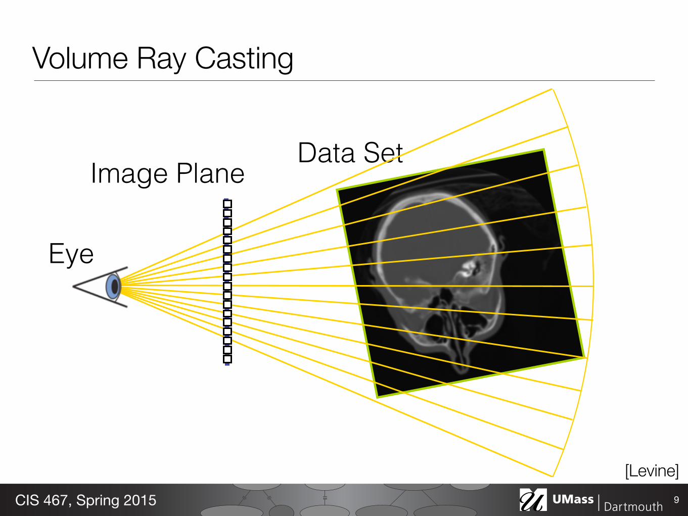
Object order approachImage Plane

Data Set

Eye

Volume Ray Casting


[Levine]

Transfer Functions


Human Tooth CT

f

RGBSimple (usual) case: Map data value f to color and opacityα

Transfer Functions (TFs)• Need to map scalar value to a color (c) and opacity (α) • Remember, we composite using the over operator • Can use other information (e.g. gradient density) in multidimensional

transfer functions

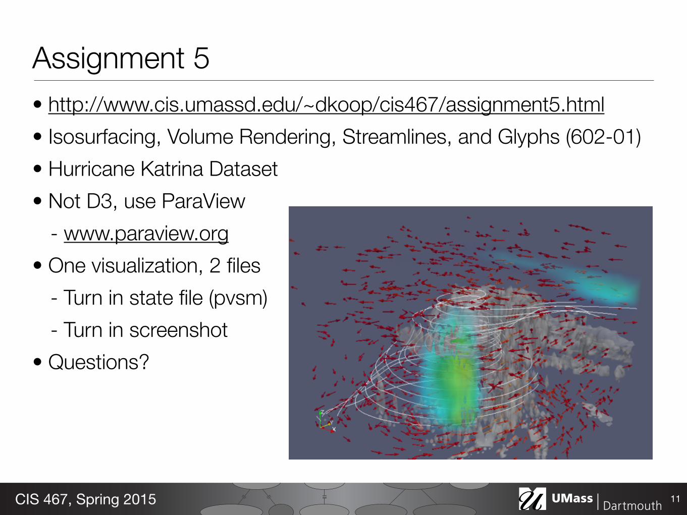
Assignment 5• http://www.cis.umassd.edu/~dkoop/cis467/assignment5.html • Isosurfacing, Volume Rendering, Streamlines, and Glyphs (602-01) • Hurricane Katrina Dataset • Not D3, use ParaView

- www.paraview.org • One visualization, 2 files

- Turn in state file (pvsm) - Turn in screenshot

• Questions?


http://www.cis.umassd.edu/~dkoop/cis467/assignment5.html

http://www.paraview.org

Final Exam• Thursday, May 7, 11:30am-2:30pm • Cumulative with emphasis on topics covered after the midterm • Topics since midterm: Maps, Color & Perception, Interaction,

Multiple Views, Aggregation, Focus+Context, Sets, Text, Scalar Fields, Vector Fields

• Textbook: Chapters 8, 10-14 • We have covered more details than in the book on: Sets, Text,

Maps, Scalar & Vector Fields • Format: Multiple Choice, Matching + Free Response


s0

2

4�00 �01 �02

�10 �11 �12

�20 �21 �22

3

5

2

4v0

v1

v2

3

5



Scalar Fields Vector Fields Tensor Fields(Order-1 Tensor Fields)(Order-0 Tensor Fields) (Order-2+)


Scalar

Vector Fields

Vector Tensor

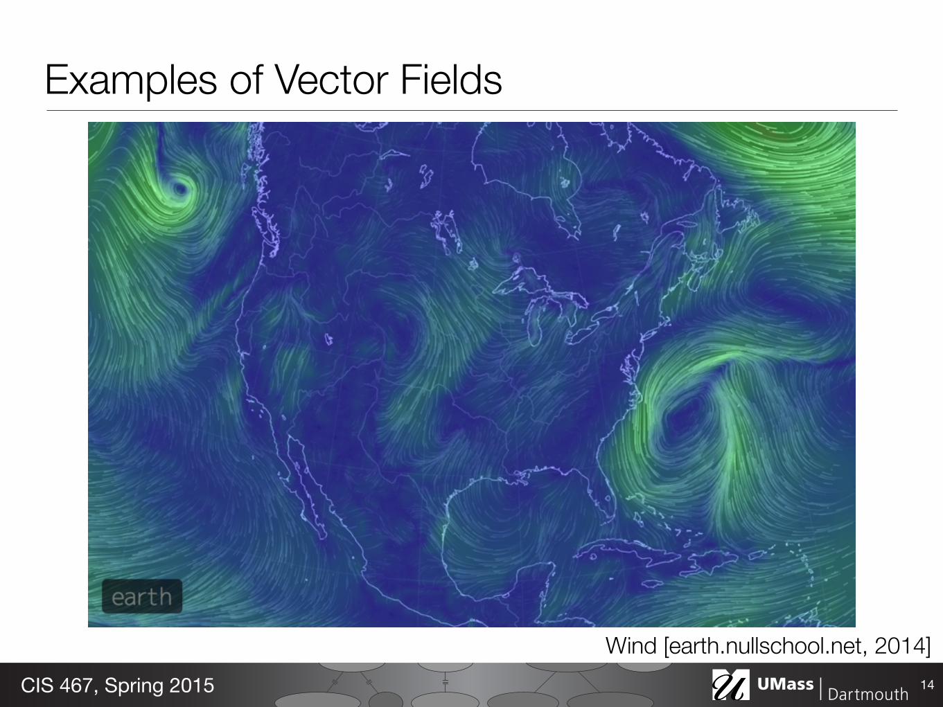
Wind [earth.nullschool.net, 2014]

Examples of Vector Fields


Wind [earth.nullschool.net, 2014]



Computational Fluid Dynamics [newmerical]





Figure 14: LIC image of the ground surface at timestep 200. The bottom 2 images show increasinglyclose-up views of the field.

sualization. We will therefore also investigate the use of agraphics-enhanced PC cluster as a dedicated visualizationserver. The question then is whether our I/O strategies cankeep up with hardware accelerated rendering.

AcknowledgmentsThis work has been sponsored in part by the U.S. NationalScience Foundation under contracts ACI 9983641 (PECASEaward), ACI 0325934 (ITR), ACI 0222991, and CMS-9980063;and Department of Energy under Memorandum AgreementsNo. DE-FC02-01ER41202 (SciDAC) and No. B523578 (ASCIVIEWS). Pittsburgh Supercomputing Center (PSC) pro-vided time on their parallel computers through AAB grantBCS020001P. The authors are grateful to Rajeev Thakurfor his technical advice on using MPI-IO, Jacobo Bielak andOmar Chattas for providing the earthquake simulation data,and especially Paul Krystosek for his assistance on settingup the needed system support at PSC.

8. REFERENCES[1] J. Ahrens and J. Painter. E�cient sort-last rendering

using compression-based image compositing. InProceedings of the 2nd Eurographics Workshop onParallel Graphics and Visualization, pages 145–151,1998.

[2] H. Bao, J. Bielak, O. Ghattas, L. F. Kallivokas, D. R.O’Hallaron, J. R. Shewchuk, and J. Xu. Large-scalesimulation of elastic wave propagation inheterogeneous media on parallel computers. ComputerMethods in Applied Mechanics and Engineering,152(1–2):85–102, Jan. 1998.

[3] H. Bao, J. Bielak, O. Ghattas, D. R. O’Hallaron, L. F.Kallivokas, J. R. Shewchuk, and J. Xu. Earthquakeground motion modeling on parallel computers. InSupercomputing ’96, Pittsburgh, Pennsylvania, Nov.1996.

[4] W. Bethel, B. Tierney, J. Lee, D. Gunter, and S. Lau.Using high-speed WANs and network data caches toenable remote and distributed visualization. InProceedings of Supercomputing 2C00, November 2000.

[5] B. Cabral and L. Leedom. Imaging vector fields usingline integral convolution. In SIGGRAPH ’93Conference Proceedings, pages 263–270, August 1993.

[6] L. Chen, I. Fujishiro, and K. Nakajima. Parallelperformance optimization of large-scale unstructureddata visualization for the earth simulator. InProceedings of the Fourth Eurographics Workshop onParallel Graphics and Visualization, pages 133–140,2002.

[7] W. Daniel, E. Gordon, and E. Thomas. Atexture-based framework for spacetime-coherentvisualization of time-dependent vector fields. InProceedings of IEEE Visualization 2003 Conference,pages 107–114, 2003.

[8] W. Gropp, E. Lusk, and R. Thakur. UsingMPI-2–Advanced Features of the Message PassingInterface. MIT Press, 1999.

Figure 14: LIC image of the ground surface at timestep 200. The bottom 2 images show increasinglyclose-up views of the field.

sualization. We will therefore also investigate the use of agraphics-enhanced PC cluster as a dedicated visualizationserver. The question then is whether our I/O strategies cankeep up with hardware accelerated rendering.

AcknowledgmentsThis work has been sponsored in part by the U.S. NationalScience Foundation under contracts ACI 9983641 (PECASEaward), ACI 0325934 (ITR), ACI 0222991, and CMS-9980063;and Department of Energy under Memorandum AgreementsNo. DE-FC02-01ER41202 (SciDAC) and No. B523578 (ASCIVIEWS). Pittsburgh Supercomputing Center (PSC) pro-vided time on their parallel computers through AAB grantBCS020001P. The authors are grateful to Rajeev Thakurfor his technical advice on using MPI-IO, Jacobo Bielak andOmar Chattas for providing the earthquake simulation data,and especially Paul Krystosek for his assistance on settingup the needed system support at PSC.

8. REFERENCES[1] J. Ahrens and J. Painter. E�cient sort-last rendering

using compression-based image compositing. InProceedings of the 2nd Eurographics Workshop onParallel Graphics and Visualization, pages 145–151,1998.

[2] H. Bao, J. Bielak, O. Ghattas, L. F. Kallivokas, D. R.O’Hallaron, J. R. Shewchuk, and J. Xu. Large-scalesimulation of elastic wave propagation inheterogeneous media on parallel computers. ComputerMethods in Applied Mechanics and Engineering,152(1–2):85–102, Jan. 1998.

[3] H. Bao, J. Bielak, O. Ghattas, D. R. O’Hallaron, L. F.Kallivokas, J. R. Shewchuk, and J. Xu. Earthquakeground motion modeling on parallel computers. InSupercomputing ’96, Pittsburgh, Pennsylvania, Nov.1996.

[4] W. Bethel, B. Tierney, J. Lee, D. Gunter, and S. Lau.Using high-speed WANs and network data caches toenable remote and distributed visualization. InProceedings of Supercomputing 2C00, November 2000.

[5] B. Cabral and L. Leedom. Imaging vector fields usingline integral convolution. In SIGGRAPH ’93Conference Proceedings, pages 263–270, August 1993.

[6] L. Chen, I. Fujishiro, and K. Nakajima. Parallelperformance optimization of large-scale unstructureddata visualization for the earth simulator. InProceedings of the Fourth Eurographics Workshop onParallel Graphics and Visualization, pages 133–140,2002.

[7] W. Daniel, E. Gordon, and E. Thomas. Atexture-based framework for spacetime-coherentvisualization of time-dependent vector fields. InProceedings of IEEE Visualization 2003 Conference,pages 107–114, 2003.

[8] W. Gropp, E. Lusk, and R. Thakur. UsingMPI-2–Advanced Features of the Message PassingInterface. MIT Press, 1999.

Earthquake Ground Surface Movement [H. Yu et. al., SC2004]



Gradient Vector Fields



Wildfire Modeling [E. Anderson]

Visualizing Vector Fields• Direct: Glyphs, Render statistics as scalars • Geometry: Streamlines and variants • Textures: Line Integral Convolution (LIC) • Topology: Extract relevant features and draw them


Glyphs• Represent each vector with a symbol • Hedgehogs are primitive glyphs (glyph is a line) • ParaView Example


Glyphs• Represent each vector with a symbol • Hedgehogs are primitive glyphs

(glyph is a line) • Glyphs that show direction and/or

magnitude can convey more information

• If we have a separate scalar value, how might we encode that?

• Clutter issues


Glyphs• For vector fields, can encode

- Direction - Magnitude - Scalar value

• Good: - Show precise local measures - Can encode scalar information as color

• Bad: - Possible sampling issues - Clutter (Occlusion): Can remove some points to help - Clutter is worse in higher dimensions


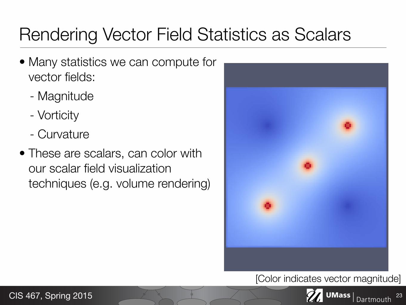
Rendering Vector Field Statistics as Scalars• Many statistics we can compute for

vector fields: - Magnitude - Vorticity - Curvature

• These are scalars, can color with our scalar field visualization techniques (e.g. volume rendering)


[Color indicates vector magnitude]

Streamlines & Variants• Trace a line along the direction of the vectors • Streamlines are always tangent to the vector field • Basic Particle Tracing:

1. Set a starting point (seed) 2. Take a step in the direction of the vector at that point 3. Adjust direction based on the vector where you are now 4. Go to Step 2 and Repeat


● Numerical integration of stream lines:

● approximate streamline by polygon xi

● Testing example: ● v(x,y) = (-y, x/2)^T● exact solution: ellipses● starting integration from (0,-1)

x

y

Example• Elliptical path • Suppose we have the actual

equation • Given point (x,y), the vector is at

that point is [vx, vy] where - vx = -y - vy = (1/2)x

• Want a streamline starting at (0,-1)


[LIC (not streamlines!) via Levine]

Euler Integration – Example2D analytic field (no need of grid and interpolation):

vx = dx/dt = −yvy = dy/dt = x/2Sample arrows:

Ground truthflows form ellipses.

0 1 2 3 4

0

1

2

Some Glyphs


[via Levine]

[x,y] → [-y, (1/2)x], Step: 0.5

Euler Integration – Example!Seed point s0 = (0 | -1 )T;current flow vector v(s0) = (1 |0 )T;dt = ½vx = dx/dt = −y

vy = dy/dt = x/2

0 1 2 3 40

1

2

Streamlines (Step 1)


[via Levine]

[x,y] → [-y, (1/2)x], Step: 0.5

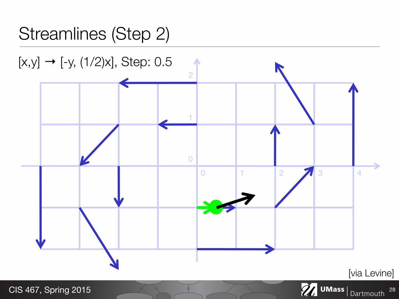
Euler Integration – Example!New point s1 = s0 + v(s0) · dt = (1/2 | -1 )T;current flow vector v(s1) = (1 |1/4 )T;vx = dx/dt = −y

vy = dy/dt = x/2

0 1 2 3 40

1

2



[via Levine]

[x,y] → [-y, (1/2)x], Step: 0.5

Euler Integration – Example!New point s2 = s1 + v(s1) · dt = (1 | -7/8 )T;current flow vector v(s2) = (7/8 |1/2 )T;vx = dx/dt = −y

vy = dy/dt = x/2

0 1 2 3 40

1

2



[via Levine]

[x,y] → [-y, (1/2)x], Step: 0.5

Euler Integration – Example!s3 = (23/16| -5/8 )T ≈ (1.44 | -0.63)T;v(s3) = (5/8 |23/32)T ≈ (0.63 |0.72)T;vx = dx/dt = −y

vy = dy/dt = x/2

0 1 2 3 4

0

1

2



[via Levine]

[x,y] → [-y, (1/2)x], Step: 0.5

Euler Integration – Example!s9 ≈ (0.20 |1.69)T;v(s9) ≈ ( -1.69 |0.10)T;

0 1 2 3 4

0

1

2



[via Levine]

[x,y] → [-y, (1/2)x], Step: 0.5

Euler Integration – Example!s19 ≈ (0.75 | -3.02)T; v(s19) ≈ (3.02 |0.37)T;clearly: large integration error, dt too large,19 steps

0 1 2 3 40

1

2



[via Levine]

[x,y] → [-y, (1/2)x], Step: 0.5

Euler Method• Seeking to approximate integration of the velocity over time• Euler method is the starting point for approximating this• Problems?



- Choice of step size is important



- Choice of step size is important- Choice of seed points are important



- Choice of step size is important- Choice of seed points are important

• Also remember that we have a field—we don't have measurements at every point (interpolation)


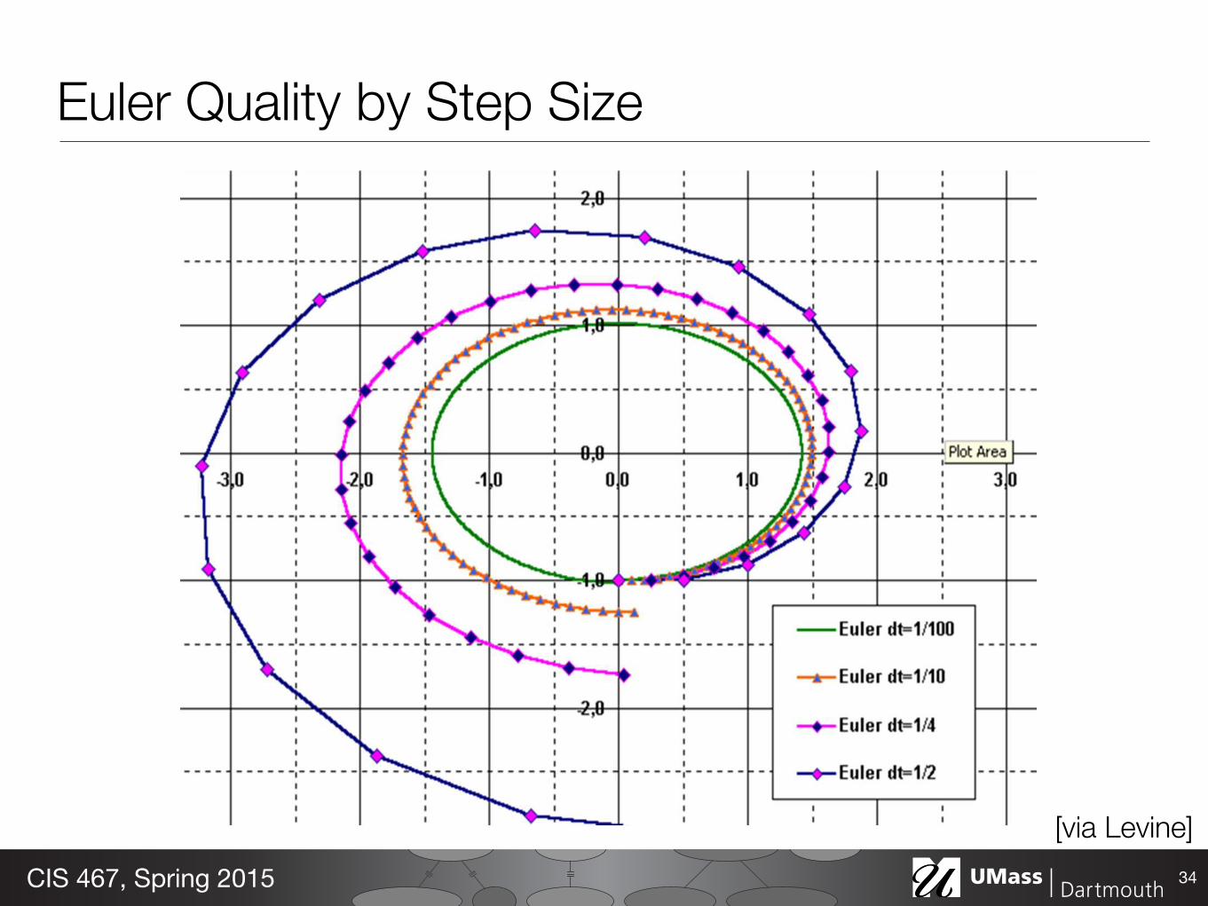
Comparison Euler, Step SizesEulerquality is proportionalto dt

Euler Quality by Step Size


[via Levine]

Numerical Integration

• How do we generate accurate streamlines? • Solving an ordinary differential equation where is the streamline, is the vector field, and is “time”

• Solution:


dL

dt= v(L(t)) L(0) = L0

L(t + �t) = L(t) +Z t+�t

tv(L(t))dt

L v t

Higher-order methods

• Euler method (use single sample)

• Higher-order methods (Runge-Kutta) (use more samples)


Z t+�t

tv(L(t))dt

v v

[A. Mebarki]

Euler vs. Runge-KuttaRK-4: pays off only with complex flows

Here approx.like RK-2

Higher-Order Comparison


[via Levine]

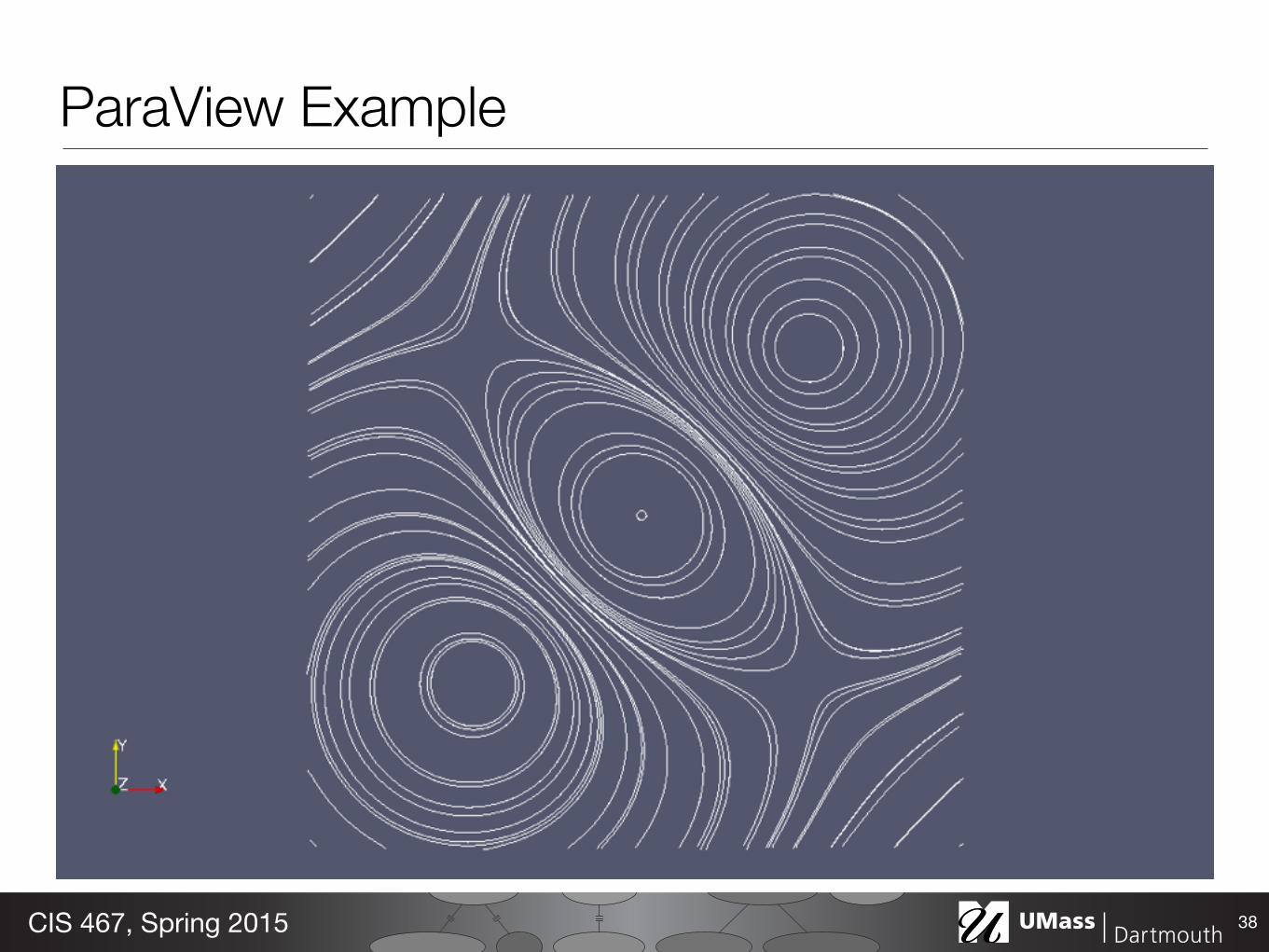
ParaView Example


Documents

CIS 467/602-01: Data Visualization