Circumpolar Deep Water Circulation and Variability in a Coupled …web.science.unsw.edu.au/~matthew/se_2006_CDW.pdf · ability along the CDW layers. The rest of this paper is divided

Circumpolar Deep Water Circulation and Variability in a Coupled Climate Model

AGUS SANTOSO AND MATTHEW H. ENGLAND

Climate and Environmental Dynamics Laboratory, School of Mathematics, University of New South Wales, Sydney, New SouthWales, Australia

ANTHONY C. HIRST

CSIRO Marine and Atmospheric Research, and Antarctic Climate and Ecosystems Cooperative Research Centre, Aspendale,Victoria, Australia

(Manuscript received 24 November 2004, in final form 3 November 2005)

ABSTRACT

The natural variability of Circumpolar Deep Water (CDW) is analyzed using a long-term integration ofa coupled climate model. The variability is decomposed using a standard EOF analysis into three separatemodes accounting for 68% and 82% of the total variance in the upper and lower CDW layers, respectively.The first mode exhibits an interbasin-scale variability on multicentennial time scales, originating in theNorth Atlantic and flowing southward into the Southern Ocean via North Atlantic Deep Water (NADW).Salinity dipole anomalies appear to propagate around the Atlantic meridional overturning circulation onthese time scales with the strengthening and weakening of NADW formation. The anomaly propagatesnorthward from the midlatitude subsurface of the South Atlantic and sinks in the North Atlantic beforeflowing southward along the CDW isopycnal layers. This suggests an interhemispheric connection in thegeneration of the first CDW variability mode. The second mode shows a localized ��S variability in theBrazil–Malvinas confluence zone on multidecadal to centennial time scales. Heat and salt budget analysesreveal that this variability is controlled by meridional advection driven by fluctuations in the strength of theDeep Western Boundary and the Malvinas Currents. The third mode suggests an Antarctic IntermediateWater source in the South Pacific contributing to variability in upper CDW. It is further found that NADWformation is mainly buoyancy driven on the time scales resolved, with only a weak connection with SouthernHemisphere winds. On the other hand, Southern Hemisphere winds have a more direct influence on therate of NADW outflow into the Southern Ocean. The model’s spatial pattern of ��S variability is consistentwith the limited observational record in the Southern Hemisphere. However, some observations of decadalCDW ��S changes are beyond that seen in the model in its unperturbed state.

1. Introduction

The absence of any meridional continental boundaryin the Southern Ocean (SO) allows a global interactionof water masses at these latitudes. Circumpolar DeepWater (CDW), the greatest volume water mass in theSO, is a mixture of North Atlantic Deep Water(NADW), Antarctic Bottom Water (AABW), andAntarctic Intermediate Water (AAIW), as well as re-circulated deep water from the Indian and PacificOceans (e.g., Wüst 1935; Callahan 1972; Georgi 1981;Mantyla and Reid 1983; Charles and Fairbanks 1992;

You 2000). Besides its role in the stability of the SOmarine environment (e.g., Prézelin et al. 2000) and inthe atmospheric carbon cycle (Sigman and Boyle 2000;McNeil et al. 2001), CDW is an important SO watermass as its upper and lower branches, namely, UpperCircumpolar Deep Water (UCDW) and Lower Cir-cumpolar Deep Water (LCDW), are further trans-formed into lighter AAIW and denser AABW, respec-tively (e.g., Döös and Coward 1997; Sloyan and Rintoul2001). The formation and circulation of these watermasses form an important component of the globalthermohaline overturning and thus of the global cli-mate system (for a review see Weaver and Hughes1992; Schmitz 1995). Understanding the natural vari-ability of CDW is therefore important for improvingour knowledge of climate variability and the detectionof climate change in the deep ocean.

Corresponding author address: Agus Santoso, School of Math-ematics, University of New South Wales, Sydney, NSW 2052,Australia.E-mail: [email protected]

AUGUST 2006 S A N T O S O E T A L . 1523

© 2006 American Meteorological Society

JPO2930

The southward outflow of NADW through the SouthAtlantic (SA) sector of the SO is an important fea-ture of the global thermohaline circulation. A DeepWestern Boundary Current (DWBC) stretching fromthe North Atlantic (NA) southward into the SA trans-ports a large volume of NADW from its formation re-gion into the SO. Several observational studies havedocumented the spatial temperature–salinity (��S)variation of outflowing NADW and its byproducts inthe Indian, Pacific, and Southern Oceans. In the north-ern NA, NADW has a range of ��S properties of 1.9°–3.6°C and 34.89–34.97 psu contributed from varioussources such as Labrador Sea water, Norwegian–Greenland Sea, and the Denmark Strait overflow wa-ters (Talley and McCartney 1982; Swift 1984; Dick-son and Brown 1994). As NADW is advected intothe SA, its ��S decreases to about 2°–3°C and 34.70–34.85 psu between 2000- and 3000-m depths at appro-ximately 40°S in the southwestern Atlantic, due tomixing with colder and fresher CDW (e.g., Reid et al.1977; Maamaatuaiahutapu et al. 1992; Tsuchiya et al.1994).

Once in the SO, waters originally from the deep NAenter the Indian Ocean south of Africa. On the �2 �36.92 kg m�3 density surface, Mantyla and Reid (1995)found that CDW within the Antarctic CircumpolarCurrent (ACC) has salinity of 34.78 psu at the tip ofSouth Africa. The ��S signature decreases farther east-ward into the Pacific where salinity is found in therange of 34.70–34.74 at 1500–2500-db levels (Reid1986). After CDW has flowed with the ACC from thePacific sector through the Drake Passage, some por-tion of the CDW then joins the deep branch of theMalvinas (Falkland) Current northward into the Bra-zil–Malvinas confluence zone (BMCZ) where the firstinteraction between CDW and outflowing NADWtakes place (e.g., Gordon 1989; Larqué et al. 1997;Stramma and England 1999). The remaining portion ofCDW continues to flow eastward with the ACC to-gether with the eastward deflection of the southwardDWBC advecting a NADW signature into the Indiansector.

Despite the documentation of ��S properties andcirculation of CDW, the extent of its variability remainsrelatively unknown. The short temporal record andsparsity of observations confound existing knowledgeof CDW variability, exacerbated by the slow processescharacterizing the ventilation of the deep water mass.Though deep ocean sediments and isotope samples pro-vide a long temporal record, data coverage is verysparse so their usage is limited in providing clues on thevariability of the thermohaline circulation (e.g., Charlesand Fairbanks 1992; Frank et al. 2002). Direct observa-

tions of ��S variations within the NADW/CDW den-sity class have been documented, in some locations inthe Southern Hemisphere (SH), but they are still cur-rently limited to decadal time scales (e.g., Johnson andOrsi 1997; Bindoff and McDougall 2000; Shaffer et al.2000; Arbic and Owens 2001).

Climate models integrated over millennia featuringrealistic climate feedbacks and global water masses area convenient tool for understanding the dynamics andevolution of deep water properties and circulation. Inthis paper we analyze CDW variability on decadal tocentennial time scales in a fully coupled ocean–atmo-sphere–ice–land surface model. The signal of NADWpropagation into the SO in response to the onset ofdeep water formation in the NA has been documentedby Goodman (1998, 2001) using an ocean only model.Thermohaline oscillations in ocean models have alsobeen studied by Mikolajewicz and Maier-Reimer(1990), Pierce et al. (1995), Osborn (1997), and Weijerand Dijkstra (2003). Our study, however, is the first toassess CDW variability in a fully coupled climatemodel, focusing on CDW ��S variability. While ourcentral goal is to assess CDW hydrographic variability,this naturally requires an analysis of circulation vari-ability along the CDW layers. The rest of this paper isdivided as follows. We begin with a description of themodel and the methods of analysis in section 2. Anoverview of model CDW ��S properties and circula-tion is provided in section 3. The CDW variability andthe driving mechanisms are described in section 4 andsection 5, respectively. The study is summarized in sec-tion 6.

2. Methodology

a. The coupled model

We analyze 1000 yr of data from the latter stages ofthe Commonwealth Scientific and Industrial ResearchOrganisation (CSIRO) 10 000-yr natural preindustrialCO2 coupled ocean–atmosphere–ice–land surfacemodel. The model is an updated version of the coupledmodel described in Hirst et al. (2000). Earlier develop-ment and coupling of the model are documented inGordon and O’Farrell (1997). Recent studies utilizingthe model can be found, for example, in O’Farrell(2002) and Santoso and England (2004). The atmo-spheric model has full diurnal and annual cycles, gravitywave drag, a mass flux scheme for convection, semi-Lagrangian water vapor transport, and a relative hu-midity–based cloud parameterization. The land compo-nent employs the soil-canopy model parameterizationof Kowalczyk et al. (1994). The sea ice model includes

1524 J O U R N A L O F P H Y S I C A L O C E A N O G R A P H Y VOLUME 36

dynamics and thermodynamics and is fully described inO’Farrell (1998). The ocean model is based on theBryan–Cox code (Cox 1984) with horizontal resolutionmatching that of the atmospheric component, namely,approximately 3.2° latitude and 5.6° longitude. Theocean model has 21 vertical levels of irregular grid boxthickness. The parameterization of Gent and McWil-liams (1990) and Gent et al. (1995) of eddy-inducedtransport (GM, hereinafter) is included with zero hori-zontal background diffusivity. Air–sea flux correctionsare implemented in the coupling to reduce long-termclimate drift.

b. Deep water structure: Isopycnal layer definitions

The structure of the model’s deep water in the SO isshown in Fig. 1 (left column) showing the zonally av-eraged salinity cross section in each ocean basin pole-ward from approximately 20°S. The corresponding ob-served Levitus salinity is shown in Fig. 1 (right column)for comparison. Despite the fresher deep water in themodel than the real ocean, particularly for the lowerNADW (LNADW), the spatial structure is reasonablywell reproduced, with realistic ventilation of NADWdescribed in O’Farrell (2002). Weak LNADW forma-

FIG. 1. Zonally averaged salinity fields below 545 m in the Atlantic, Indian, and Pacific sectors in the (left) model and (right) Levituset al. (1994). The �2 isopycnal surfaces are shown by the thick dashed contours. The UCDW and LCDW in the model are analyzedalong isopycnal layers bounded by �2 � 36.70–36.80 and 36.80–36.90 kg m�3, respectively. The �2 layers in the observed field atisopycnal depths matching the model’s isopycnal layers are included in the right column.


tion is a common problem in ocean GCMs, resultingfrom poor representation of overflow processes southof the Greenland Sea (England and Holloway 1998).This enables stronger than observed AABW intrusioninto the NA. This in turn yields a shallower salinitymaximum core layer in the model relative to observa-tions, with fresher than observed deep water. UpperNADW (UNADW), in contrast, is well resolved by themodel; it is this shallower variety of NADW that is ofgreater interest in the present study. The outflow ofrelatively saline UNADW in the Atlantic is seen in themodel as in the observed with decreasing salinity as itupwells poleward and mixes with the fresher CDW.Traces of the salinity maximum are also observed in theIndian and Pacific sectors. As noted by Hirst et al.(2000), the inclusion of the GM parameterization re-sults in a more realistic CDW density as compared withthe model without GM. Eddy fluxes play an importantrole in the southward flushing of UCDW (Speer et al.2000).

Our study focuses on the salinity maximum deep wa-ter layer above about 3000 m but at depths below 1000m isolated from the direct influence of air–sea interac-tions. The potential density layer referenced to 2000 db�2 � 36.70–36.90 kg m�3 (�n � 27.70–27.92) is chosento inscribe the NADW layer and approximately cap-tures the core of CDW in the model. Note that thelocally referenced density at 2000 db is a reasonableapproximation of neutral density surfaces for deep wa-ter analysis within the 1000–3000-m depth range. Thislayer corresponds to �2 � 36.80–37.02 kg m�3 (�n �27.82–28.07) in the observed at approximately the same

depth levels (Fig. 1; right column), implying insuffi-ciently dense deep water in the model, a problem typi-cal of coarse-resolution ocean GCMs (England andHirst 1997; Hirst et al. 2000). As also noted in Bianchiet al. (1993), CDW coexists with NADW within the�2 � 36.75–37.15 kg m�3 density range (estimated fromReid et al. 1977; their Fig. 6b), which includes our ob-served CDW density layer �2 � 36.80–37.02 kg m�3

(Fig. 1; right column).We further divide the model’s CDW layer into an

upper and lower part at �2 � 36.80 kg m�3, which ap-proximately corresponds to �2 � 36.94 kg m�3 in theobservations (see Fig. 1; right column). This choice oflayer separation is similar to that of Mémery et al.(2000) where UCDW and UNADW in the southwest-ern Atlantic are observed to overlap over �2 � 36.72–36.95 kg m�3 above 2000-m depth. Reid et al. (1977)and Sievers and Nowlin (1984), on the other hand, at-tributed �2 � 36.97 kg m�3 as the upper limit ofLCDW, which is also a separation surface betweenUNADW and LNADW (Reid et al. 1977). The waterbelow the separation layer is then regarded as LCDW,which intercepts, in its upper branch, the core of thesalinity maximum of NADW. For example, García etal. (2002) observed a salinity maximum of up to 34.72psu in the LCDW layer in the Drake Passage. Note thatthe CDW layers chosen in our analyses also coincidewith the salinity maximum in the Indian and Pacificbasins (Fig. 1). The position of the isopycnal layers rela-tive to the Atlantic basin meridional overturningstreamlines is shown in Fig. 2. Both the UCDW andLCDW layers coincide with the outflowing NADW

FIG. 2. Atlantic meridional overturning (Sv) averaged over 1000 model years. The thick dashed contours mark the �2 � 36.70–36.80and �2 � 36.80–36.90 kg m�3 layers. Contour interval for the meridional overturning is 2 Sv.


into the SO, with the LCDW layer capturing a smallportion of the upper part of the bottom water recircu-lation cell. The overturning features of the model havebeen discussed in Hirst et al. (2000) and are thus notelaborated here. However, note that in addition to thedeep overturning cell in the NA, the Atlantic bottomrecirculation is also weaker than that inferred from theobservations of Sloyan and Rintoul (2001) and Talley(2003).

c. Spatiotemporal variability analyses

We analyze annually averaged ocean variables sinceour focus is on deep water depths, where seasonal ef-fects are negligible. The analyzed variables include1000-yr ocean potential temperature (�), salinity (S),and horizontal velocities u � (u, �) from the latter partof the 10 000-yr run. We focus mainly on the area southof 20°S, which covers the SO domain. The ocean vari-ables are linearly interpolated vertically onto discretepotential density surfaces at 0.01 kg m�3 intervals be-tween �2 � 36.70 and 36.90 kg m�3, inclusive. Averagedproperties along the isopycnal surfaces are obtained foreach of the �2 � 36.70–36.80 kg m�3 and �2 � 36.80–36.90 kg m�3 layers to represent the UCDW andLCDW, respectively (section 2b). The isolation ofCDW from the surface is ensured by applying the layeraveraging only when the uppermost surface is at1000-m depth or deeper (see Fig. 3). The mean positionof the UCDW and LCDW isopycnal layers are labeledas �UCDW and �LCDW, respectively.

A standard empirical orthogonal function (EOF)analysis is employed to decompose ��S variabilityalong �UCDW and �LCDW into orthogonal modes, each

accounting for a portion of the total data variance. Thespatial and temporal evolution of each variability modeare obtained from its eigenvector and expansion coef-ficient (also known as the principal component), re-spectively. For a detailed description of the EOF tech-nique, the reader is referred to Preisendorfer (1988).Correlation and spectral analyses are implemented toreveal the temporal characteristics and relationshipsbetween variables. The spectral analyses are based onthe Thomson multitaper method described in Percivaland Walden (1993) and Mann and Lees (1996) for bet-ter statistical significance. The computation of cor-relation confidence level coefficients is described inSciremammano (1979). We also analyze complex EOFs(CEOFs) in order to reveal the propagation of anoma-lies [see, e.g., Horel (1984) for a description of theCEOF technique]. Heat–salt budget analyses are con-ducted to help to identify mechanisms controllingCDW ��S variability (for details see the appendix).

3. Model CDW: Mean properties and circulation

a. Upper layer

Figures 4a and 4b show the mean ��S on �UCDW inthe model and observed (Levitus and Boyer 1994; Levi-tus et al. 1994), respectively. The mean circulation andisopycnal layer depth in the model are presented in Fig.4c (the labeled locations, R1–R4, are used in section 4ato describe the spatial distribution of deep water ��Svariability at certain locations). The relatively salineand warm UNADW advected by the southwardDWBC in the southwestern Atlantic at 20°�33°Sshows ��S of �4.0°C and 34.84 psu in the model. Theobserved shows colder and slightly fresher UNADW of�3.0°C and 34.81 psu. The UCDW layer in this regionis found at a mean depth of about 1700 m. The purestconcentration of UNADW is confined off the coast ofBrazil with ��S extrema of 4.1°C and 34.86 psu in themodel at about 30°S, 40°W, which is warmer andfresher than the observed ��S of 3.7°C and 34.94 psu(see also Reid et al. 1977, their Fig. 3a).

Temperature and salinity along �UCDW decreasegradually because of mixing as UCDW flows into theIndian and Pacific sectors. In the Agulhas Basin at 40°S,22°E (around R2), the model’s UCDW has average��S of 3.1°C and 34.67 psu, which is again warmer andfresher than the observed (2.6°C and 34.73 psu). TheUCDW further cools and freshens eastward. Themodel captures the westward flow from the South Aus-tralian Basin toward the east coast of Africa via theIndian Ocean interior, as also suggested by the obser-vations of Mantyla and Reid (1995) on �2 � 36.92.

The spatial ��S variations in the Pacific sector are

FIG. 3. Definition of Circumpolar Deep Water layers used in themodel analysis. Linear interpolation and averaging are applied foreach layer wherever the upper boundary is below 1000-m depth.The core surfaces are labeled as �UCDW and �LCDW, respectively.


weaker than in the other ocean basins in both modeland observations. To the south of New Zealand toDrake Passage along about 53°S, ��S decreases lessrapidly from �2.2°C, 34.51 psu to 2.1°C, 34.48 psu inthe model and from �2.2°C, 34.65 psu to 2.1°C, 34.64psu in the observed (see also Callahan 1972; Sieversand Nowlin 1984). The UCDW variety in the Pacificsector is the coldest and freshest because of mixing withrecirculated interior waters from the Pacific basin.There is a mean southward flow at the western bound-

ary (�0.3 cm s�1) in the model along the LouisvilleSeamount Chain (20°–40°S, 170°W) joining the ACCtoward the Drake Passage. This flow is observed in thereal ocean, for example, by Wunsch et al. (1983), Whit-worth et al. (1999), and Wijffels et al. (2001).

As seen in observations, the model captures flowthrough the Drake Passage being deflected northwardin the Malvinas Current into the BMCZ where it meetsthe southward flowing DWBC. Because of the strongersignature of NADW and the colder and fresher UCDW

FIG. 4. Mean potential temperature and salinity along �UCDW in (a) the model and (b) the observed Levitus and Boyer (1994) andLevitus et al. (1994) climatology. The potential temperature contour interval is 0.15°C. The isopycnal layer is defined over a completeset of discrete �2 values with an interval of 0.01 kg m�3 from 36.70 to 36.80 kg m�3 inclusive for the model data and 36.80 to 36.94 kgm�3 for the observed data (see Figs. 1 and 3). The color scale for the model output shown in (a) has been adjusted to match the salinityrange of the observed (b); however, there remains an offset in the salinity scale in (a) and (b). (c) Mean circulation on �UCDW. Toenhance visibility of the circulation features at depth, the current vectors have been rescaled by |log10(speed)| � 0.1. The mean isopycnaldepths are shown by the color-scaled contours in (c). The locations R1–R4 are marked with filled magenta circles.


Fig 4 live 4/C

in the model, the lateral ��S gradient in the BMCZappears to be larger than in the observed (Figs. 4a,b).

b. Lower layer

The ��S spatial distribution on �LCDW is for themost part similar to that on �UCDW for both the modeland observations (Figs. 5a,b). The water along thisisopycnal layer is generally colder and fresher in themodel relative to the observed. Similar circulation pat-terns to the upper layer are also observed on �LCDW

(Fig. 5c), characterized by the convergence of theDWBC and the Malvinas Current in the BMCZ beforejoining the ACC and flowing into the other SO sectors.Topographical obstructions are apparent on �LCDW.

The LCDW flow in the ACC is partially obstructed bythe Kerguelen Plateau (40°–57°S, 70°–80°E). Mantylaand Reid (1995) suggest that flow on the �2 � 37.00surface separates into three streams as it approachesthe Kerguelen Plateau. The anticyclonic shear in theSouth Australian Basin and the northward flow in theMascarene Basin (20°–40°S, 50°E) are also consistentwith the observations of Mantyla and Reid (1995). Inthe Pacific, northward deflections of the ACC occuralong Chatham Rise (southeast of New Zealand) up to45°S before turning eastward again. This is consistentwith the geostrophic flow in Reid (1986) at 2000–2500-db levels. The northward flow into the Tasman Sea asobserved in Reid (1986) is also resolved, as well as thelarge anticyclonic gyre in the South Pacific and the

FIG. 5. As in Fig. 4 but for �LCDW. Figure 1 shows the layer definition for �LCDW in the model and observed (see also Fig. 3).


Fig 5 live 4/C

southward eastern boundary flow along the coast ofChile (80°W).

c. Summary

The model mean ��S and circulation fields on thedensity layers corresponding to CDW show good over-all agreement with observations. While the salinity ofoutflowing LNADW is fresher than the observed, ren-dering LCDW to be too fresh by �0.2 psu, the spatial��S variations of CDW are qualitatively similar to ob-served climatologies. In addition, the model’s CDWflow pathways are remarkably consistent with availableestimates of deep SO circulation patterns.

4. CDW variability patterns

a. ��S properties

The spatial and temporal variability of the model’sCDW on �UCDW and �LCDW are described in this sec-tion. Figure 6 presents the spread of ��S over 1000 yrat the selected locations shown in Figs. 4c and 5c on�UCDW and �LCDW, respectively. The depths are takenas the mean depth of �UCDW and �LCDW at each loca-tion. We focus our analysis on the along-isopycnal vari-ability of CDW. Nonetheless, some reference is alsomade to the along-isobar variability, as this gives insightinto the effect of isopycnal vertical excursions in re-sponse to the ��S fluctuations (Bindoff and McDougall1994; see also, e.g., Arbic and Owens 2001; Wong et al.2001).

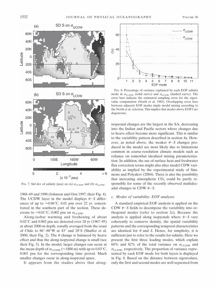
Variability in both �UCDW and �LCDW ��S decreasesgradually eastward from the Atlantic sector (Fig. 6).This is further illustrated in a standard deviation analy-sis (Fig. 7), showing a decrease in ��S variability intothe Indian and Pacific basins. This variability patternresembles the pathway of NADW outflow into the SO(see, e.g., Sen Gupta and England 2004). Note also thatthe strongest variability in the Southern Hemisphere islocalized in the BMCZ.

On �UCDW (Fig. 6), the along-isopycnal ��S rangedecreases gradually from 0.19°C, 0.036 psu at R1 (At-lantic) to 0.04°C, 0.006 psu at R4 (Pacific). The ��Srange along isobars decreases from 0.21°C, 0.036 psu atR1 to 0.07°C, 0.008 psu at R4. The magnitude of vari-ability in the lower layer is smaller than in the upperlayer (Fig. 6), but with similar geographic trends. Aninteresting feature of Fig. 6 is that the along-isobar ��Svariations at R1 (Atlantic Ocean) are in near densitycompensation. On the other hand, there is a larger di-apycnal spread at fixed depth at R2, R3, and R4 (Indi-an–Pacific Oceans) marked by the dominance of heaveeffect (see appendix). This spatial distribution of the

changes also appears consistent with the observationsdiscussed in section 4b. The changes due to the heaveeffect are shown by the heat–salt budget analyses (seeappendix) to balance the vertical fluxes. On the otherhand, changes along isopycnals are mainly attributed tohorizontal advection transmitting anomalies over largespatial and temporal scales. It should be noted here thatgeneration of ��S anomalies along isopycnals can beattributed to one or a combination of the followingmechanisms: 1) air–sea flux variations at water-massformation regions (e.g., Arbic and Owens 2001), 2)anomalous advection across ��S fronts (Schneider2000; Rintoul and England 2002), and 3) ��S and/orvolume variability of adjacent water masses (Johnsonand Orsi 1997), which also causes heaving of isopycnals.Isopycnal heaving can also result from changes in therate of gyre spin and baroclinic wave propagation. Inthe following sections we further examine the modesand mechanisms of CDW variability.

b. Comparison with observations: Decadal changes

This section provides a brief overview of the ob-served decadal changes in CDW in the SO. We willcompare these changes with the model’s largest magni-tudes of decadal ��S change observed over the courseof the 1000-yr model simulations. Note, however, that adetailed comparison is not straightforward here. First,the model’s coarse resolution renders it a more dampedsystem relative to the real ocean with its rich structuresof ��S variability. Second, while the model is run withconstant CO2, the observed changes occur during anera of increasing anthropogenic CO2. This second fac-tor is perhaps less significant as modern-day CDW is abyproduct of water masses formed as long as centuriesago. In addition, by examining a constant CO2 run, wecan isolate natural, not forced, modes of CDW variabil-ity.

Basin-averaged along-isobar warming and salinationof �0.2°C (100 yr)�1 and 0.1 psu (100 yr)�1 were ob-served at �2000-m depth over 1925 to 1959 along 32°Sin the southwestern Atlantic (Arbic and Owens 2001;their Figs. 3 and 4). The along-isobar changes consist ofmostly changes along isopycnal (their Fig. 9). The cor-responding changes in the model at the local meandepth of �UCDW (�1700 m) display zonally averagedmagnitudes of up to 0.1°C (100 yr)�1 and 0.02 psu (100yr)�1. The Arbic and Owens (2001) salinity changeswould therefore appear beyond natural variations inCDW.

Temperature–salinity changes between 1962 and1987 across the Indian Ocean at �32°S have been docu-mented by Bindoff and McDougall (2000). Basin-averaged cooling and freshening along isobars are ob-


served at about 2000-m depth of the order of 0.05°Cand 0.005 psu (see their Fig. 6). They suggest that thechanges are due to heaving of isopycnals. The corre-sponding changes in the model are smaller with basin-averaged values on �UCDW of up to �0.02°C and 0.002psu (25 yr)�1. Along-isopycnal change in the model isabout one-half that of the along-isobar change for � and

is comparable in magnitude for S, suggesting that heaveeffects account for the density difference due to �change (see also Bindoff and McDougall 2000; theirFig. 10).

In the Pacific, pronounced cooling and freshening ofup to 0.07°C and 0.01 psu along deep density surfacesbetween 40° and 20°S are found along 170°W between

FIG. 6. Model 1000-yr ��S scatterplots on isopycnal surfaces (crosses) at the specific locations shown in Figs. 4c and 5c (marked asR1–R4) on (left) �UCDW and (right) �LCDW. The corresponding ��S properties at fixed depths (taken as the mean depth of theisopycnal layer) are marked with dots.


1968–69 and 1990 (Johnson and Orsi 1997; their Fig. 4).The UCDW layer in the model displays ��S differ-ences of up to �0.06°C, 0.01 psu over 22 yr, concen-trated in the southern part of the section. These de-crease to �0.01°C, 0.002 psu on �LCDW.

Along-isobar warming and freshening of about0.02°C and 0.002 psu are detected over 28 yr (1967–95)at about 2000-m depth, zonally averaged from the coastof Chile to 86°–88°W at 43° and 28°S (Shaffer et al.2000; their Fig. 2). The � change is balanced by heaveeffect and thus the along-isopycnal change is small (seetheir Fig. 3). In the model, larger changes can occur atthe mean depth of �UCDW (�1800 m) with up to 0.03°C,0.001 psu for the corresponding time period. Muchsmaller changes occur in along-isopycnal space.

It appears from the studies above that along-

isopycnal changes are the largest in the SA, decreasinginto the Indian and Pacific sectors where changes dueto heave effect become more significant. This is similarto the variability pattern described in section 4a. How-ever, as noted above, the weaker ��S changes pro-duced in the model are most likely due to limitationscommon in coarse-resolution climate models such asreliance on somewhat idealized mixing parameteriza-tion. In addition, the use of surface heat and freshwaterflux correction terms might also alter model CDW vari-ability as implied by the experimental study of Sim-mons and Polyakov (2004). There is also the possibilitythat increasing atmospheric CO2 could be partly re-sponsible for some of the recently observed multidec-adal changes in CDW ��S.

c. Modes of variability: EOF analyses

A standard empirical EOF analysis is applied on theCDW ��S fields to decompose the variability into or-thogonal modes (refer to section 2c). Because theanalysis is applied along isopycnals where ��S varycoherently to conserve density, the spatial variabilitypatterns and the corresponding temporal characteristicsare identical for � and S. Hence, for simplicity, it issufficient just to refer to the results for salinity. Here wepresent the first three leading modes, which explain68% and 82% of the total variance on �UCDW and�LCDW, respectively. The proportion of variance repre-sented by each EOF mode for both layers is displayedin Fig. 8. Based on the distance between eigenvalues,only the first and second modes are well separated from

FIG. 7. Std dev of salinity (psu) on (a) �UCDW and (b) �LCDW.

FIG. 8. Percentage of variance explained by each EOF salinitymode in �UCDW (solid curve) and �LCDW (dashed curve). Theerror bars indicate the estimated sampling error for the eigen-value computation (North et al. 1982). Overlapping error barsbetween adjacent EOF modes imply modal mixing according tothe North et al. criterion. This implies that modes above EOF3 aredegenerate.


their neighboring modes. Higher modes are more likelyto be affected by “effective degeneracy” and “mixing”(refer to Fig. 8 and caption); thus physical interpreta-tion for these modes can be difficult (North et al. 1982).The spatial patterns of the first three modes are dis-played in Fig. 9. The corresponding temporal charac-teristics are shown in Fig. 10, presented by the principalcomponent (PC) time series and their correspondingpower spectra.

EOF1 exhibits an interbasin-scale variability ofCDW salinity originating from the SA oscillating onmulticentennial time scales as shown by the character-istic time series (PC1). The UCDW mode has PacificOcean salinity anomaly out of phase with the SA. Inboth layers the major signature is in the Atlantic sector,decreasing in magnitude eastward along the ACC. Thecorresponding power spectra display signals at centen-nial–millennial time scales with a dominant period of�330 yr. Interdecadal variability is stronger in PC1 forthe UCDW layer, which is due to the shallow outflowlevel of NADW. From its spatial characteristics, EOF1is likely to be related to variability in the NADW prop-erties flowing into the SO (discussed further in section 5a).

The spatial pattern of EOF2 (Fig. 9) shows large vari-ance in the BMCZ where UNADW advected by theDWBC mixes with the fresher and colder CDW ad-vected northward by the Malvinas Current. The local-ized region of the largest variability is marked by a boxin Fig. 9 (EOF2) situated at the BMCZ. A weaker and

out-of-phase pattern can be seen in the region from thesoutheastern Atlantic into the circumpolar region southof Australia. The EOF2 mode is characterized by sig-nals at interdecadal–centennial time scales with a dom-inant variability at 100-yr period on both �UCDW and�LCDW (Fig. 10). There is a 30-yr peak in the powerspectrum for PC2 in �UCDW, which is virtually absent in�LCDW. The mechanisms controlling this second EOFmode of variability are described in section 5b.

The third mode in each layer explains less than 10%of the total variance. EOF3 for �UCDW reveals variabil-ity sourced in the South Pacific spreading northward. Incontrast, EOF3 for �LCDW shows a wavenumber-1mode of ��S variability on interdecadal to multicen-tennial time scales (Fig. 10). The mechanism for thisvariability mode is briefly described in section 5c.

The three EOF modes above are retained by com-plex EOF (CEOF) analyses as shown in Fig. 11a pre-senting the CEOF spatial maps on �UCDW at 90° phaseintervals. The CEOF maps for �LCDW are not presentedhere as they resemble their EOF counterparts and showsimilar CEOF patterns as �UCDW. The spatial phasemaps (Fig. 11b) show eastward propagation of anoma-lies in the SO, as well as northward propagation into theIndian and Pacific basins. A more extended EOF analy-sis of ��S fields from a 1600-yr dataset taken fromearlier model years also captures variability modes withsimilar spatial and temporal characteristics as themodes described above, although with different

FIG. 9. Spatial maps of the first three EOF modes of salinity on (top) �UCDW and (bottom) �LCDW, accounting for 68% and 82% ofthe total S variance, respectively. The values of the eigenvectors have been normalized to unity so that the spatial maps span valuesbetween �1 and 1, and hence the principal components (Fig. 10, left column) correspond to the actual magnitude of the variabilityassociated with each mode. The box in the EOF2 map indicates the BMCZ.


Fig 9 live 4/C

amounts of variance explained by each mode (figurenot shown). Thus, the modes described are robust andare likely to represent physical processes in the model.Last it may be noted that the combination of theEOF1–EOF3 spatial patterns approximately makes upthe overall CDW variability pattern as shown by thestandard deviation maps in Fig. 7. This is because thefirst three EOFs account for a significant component ofthe total ��S variability.

5. Variability mechanisms

a. First mode

The spatial pattern of the first ��S variability mode(EOF1; Fig. 9) was seen to be concentrated in the SA,

decreasing eastward into the SO. This pattern suggeststhat the variability may be linked to variations inNADW ��S, originating from the formation regions inthe NA. To investigate this, we present a correlationanalysis between the first principal component (PC1)and the box-averaged salinity anomalies along isopyc-nals in a region downstream of the Labrador Basin (la-beled SNA) and another in the deep tropical region inthe SA (labeled SSA; see Fig. 12 for the respective lo-cations). The time series of PC1 and salinity at SNA, SSA

are presented in Figs. 12a,b for �UCDW and �LCDW,respectively. Note the more prominent interdecadalsignals on �UCDW in comparison with �LCDW becausethis upper layer is closer to the core of outflowingNADW (Fig. 2). The variability on interdecadal time

FIG. 10. (left) Principal component time series of EOF1–3 (PC1–3) and (right) the corresponding power spectral density for �UCDW

(thin solid line) and �LCDW (thick solid line). A log10 scale is used in frequency to give more weight to the higher-frequency signals,and the power spectra are multiplied by frequency to preserve variance.


scales is also more pronounced at SNA relative to SSA,because of the greater damping of NADW variability,via mixing, as these waters are advected away fromtheir source regions.

PC1 and salinity at SNA, SSA are correlated signifi-cantly (about 95% confidence level) at different timelags as shown in Figs. 12c and 12d. This suggests thatthe first CDW EOF mode is mainly capturing NADWspiked ��S variability originating upstream in the NA.On �UCDW SNA leads SSA by 51 yr, suggesting that theanomalies travel at �0.4 cm s�1 to cover a distance of60° latitudes over �50 yr. This is approximately themean DWBC velocity from SNA to SSA, within themodel CDW layer. Here SSA leads PC1 variability by�13 yr and SNA leads PC1 by �65 yr, again matchingthe advective time scales for NA ��S anomalies totravel into the SO. The LCDW layer exhibits margin-ally shorter lag times, for example, 49-yr lag from SNA

to SSA. This is likely due to different mixing rates in thetwo CDW layers. For example, the magnitude of vari-ability of SNA is about twice that of SSA on �UCDW,while the magnitude of the signals at SNA, SSA is com-parable on �LCDW. Thus, more damping occurs along�UCDW, accounting for the slower phase speed in thatlayer’s EOF1.

The flow of ��S anomalies out of the Atlantic can bedepicted in Fig. 13 showing a correlation map ofthe salinity field against SNA on �UCDW at increasingtime lags. The corresponding lag correlation map on�LCDW is similar to �UCDW and is thus not presentedhere. The diagram suggests a large-scale propagationof anomaly from the NA southward in the DWBCthen continuing eastward in the ACC (see also Good-man 2001). When SNA is shifted back in time by 20 yr,the lag correlation is significantly high in the regionnorth of SNA, showing that the anomaly signals indeedoriginate from the NADW formation regions. Atlonger time lags, the correlation peak propagates intothe Indian and Pacific basins, but with reduced ampli-tude as the anomalies have their characteristics dampedby mixing. As shown in the appendix, the ��S variabil-ity is controlled by meridional advection in the SAwhere along-isopycnal variability dominates, and byzonal advection in the SO where heave processes aremore intense.

It should be noted that one-half of a cycle of NADWoutflow and recirculation involves an outflow of posi-tive anomaly from the SA into the SO, and the ensuingpropagation of a negative anomaly in which theseanomalies propagate with the ACC and flow northward

FIG. 11. (a) Spatial maps of the first three CEOF modes of salinity on �UCDW shown at 90° phase intervals. The three modes accountfor �76% of the total salinity variance with COEF1, COEF2, and CEOF3 accounting for 44%, 21%, and 10%, respectively. (b) Spatialphase angle for CEOF1–3 indicating the direction of propagation at increasing angle. Phase discontinuities occur at 360°–0° because thephase is defined only between 0° and 360°.


Fig 11 live 4/C

into the Indian and Pacific basins. A negative anomalyis seen in the SA to continue the second half of thecycle (see CEOF1 spatial map in Fig. 11a, top). Wefurther note that the propagation of anomalies from theNA to the SO takes �80 yr, corresponding to a quartercycle, and thus the 330-yr peak shown in the spectra ofPC1 (Fig. 10).

Figure 14 presents a series of raw salinity anomalymaps on a meridional–vertical plane along the Atlanticwestern boundary from years 179–515 in 42-yr intervals(refer to Fig. 15 for the location of the section). A posi-tive S anomaly fills the NA in year 179 and is flushedsouthward along �UCDW and �LCDW with a decreasingmagnitude (year 305). This is then followed by the ap-pearance of a negative anomaly in the north at year 347.

The cycle continues at irregular periodicity of approxi-mately 330 yr. This corresponds to a half cycle of �160yr for an NA anomaly to propagate into the SO. Thetime scale of the propagating anomalous signals seen inFig. 13, namely, the multidecadal transit from the NAto SA, is similar to the study of Smethie et al. (2000)using chlorofluorocarbons to trace the outflow ofNADW.

Similar periodicity is also found in the Atlantic ther-mohaline circulation of the Hamburg large-scale geo-strophic ocean-only general circulation model (LSGOGCM), accompanied by a dipole salinity anomalypropagating around the meridional–vertical plane witha dominant period of 320 yr (Mikolajewicz and Maier-Reimer 1990; see their Fig. 10). The oscillation is gen-

FIG. 12. Time series PC1 and box-averaged salinity anomalies at SNA, SSA (defined over the regions indicated at left) in (a) �UCDW

and (b) �LCDW. Correlation coefficients between the variables are shown for (c) �UCDW and (d) �LCDW. The corresponding 95%confidence levels are shown for each analysis (the significance curves for SNA vs PC1 and SNA vs SSA are nearly identical).


erated by the SO “flip flop” oscillator described inPierce et al. (1995) in which NADW supplies heat tothe high latitudes of the SO, inducing deep convectionthere. The convection in turn influences the thermoha-line flow through the Drake Passage (Pierce et al.1995). As a result, the ACC variability has a stronglinear relationship with the outflow rate in the Ham-burg LSG OGCM (Mikolajewicz and Maier-Reimer1990). In addition, there is a clear teleconnection be-tween the NH and SH high-latitude oceans. In a fullycoupled model such as the one used in this study, theNADW–ACC relationship is expected to be less linear.This is confirmed by the low lagged correlation coeffi-cient between the outflow rate (or formation rate) ofNADW and the Drake Passage transport in the model(Table 1). The NADW formation rate is, however,strongly connected to the NA buoyancy, while theDrake Passage throughflow is tightly linked to theWeddell Sea buoyancy (see Table 1). Osborn (1997)showed that the nature of the oscillation can be alteredby a more realistic atmospheric thermal feedback,which is absent in the LSG model, which in turn affects

the extent of convection. The inclusion of the GM pa-rameterization, which is also known to influence con-vection, ventilation rates, and thermohaline circulationstructure (see, e.g., Hirst and McDougall 1996; Englandand Rahmstorf 1999; Hirst et al. 2000; Kamenkovichand Sarachik 2004), may further enhance the nonlin-earity observed in our model.

While the multicentennial periodicity is set by theNADW outflow time scale, it is unclear exactly whatsets the ��S anomalies in the NA. Though detailedinvestigation is beyond the scope of the paper, it isworth commenting that like the LSG model, thereseems to be an influence from the SO. This is evident byreferring to Fig. 15, which shows a composite map of Sanomaly during periods of high and low NADW for-mation rates (defined as those above/below one stan-dard deviation from the mean). Positive S anomaly oc-curs in the NA with high NADW formation rate (Fig.15a). This is followed by negative anomaly at the sub-surface down to intermediate depths in the SH, near40°S, which then propagates northward (as suggested inFig. 14, years 179–305). The converse occurs during pe-

FIG. 13. Correlation maps between global salinity fields and the box-averaged salinity at SNA (indicated by the boxed region) on�UCDW at different time lags (20-yr interval), showing a propagation of salinity anomaly in outflowing NADW. Correlation coefficientsare not shown when they fall below the 95% significance level. Note that the significance level increases with increasing time lags.


Fig 13 live 4/C

riods of low NADW formation rate (Fig. 15b, namely,negative S anomaly fills the NA water column and isaccompanied by the occurrence of a subsurface positiveS anomaly near 40°S; see also Fig. 14, years 305–431).This suggests that at least some portion of the anomalyin the NA may be sourced from the SO [via Sub-Antarctic Mode Water (SAMW) and AAIW]. Onepossible variability mechanism is through conversion ofUCDW to Antarctic Surface Water (AASW) atUCDW outcrop regions, from where AASW is furthertransformed to AAIW/SAMW via meridional Ekmantransport (Rintoul and England 2002; Santoso and En-gland 2004). These water masses eventually flow north-ward in the Atlantic to close the NADW overturningcell (Sloyan and Rintoul 2001).

While the variability in NADW formation is clearlydriven by thermohaline forcing in the NA, the evidencefor a SO wind influence as proposed by Toggweiler andSamuels (1995) is not apparent in our model. This isshown by the low correlation between NADW produc-tion rate and the northward Ekman transport at thelatitude of Cape Horn [labeled as VE

TS95 in Table 1, with

a mean of about 24 Sv (1 Sv 106 m3 s�1)]. The rela-tionship would presumably be more apparent if thermalfeedbacks were excluded (Rahmstorf and England1997). This is clearly not the case in a coupled climatemodel. The relationship between the outflow rate andthe wind transport at the southern tip of South Ameri-can (as calculated according to Toggweiler and Samuels1995) is also only weak, with a correlation coefficient of0.14. However, the influence of SH winds is more ap-parent along a slightly different path integral. In par-ticular, Nof (2003) proposed that the integral of windstress along a closed integration path, situated north ofthe ACC, connecting the tips of South America, SouthAfrica, and South Australia (Nof03; Table 1), gives anestimation of the net transport into the NA. This trans-port corresponds to a net northward interior flow, abalance between the Western Boundary Current andthe Sverdrup interior. Note that the mean of this cal-culated integrated transport neglecting friction termsaccounts for about 22 Sv, which includes the Ekmantransport, the geostrophic flow underneath, and theWestern Boundary Current transport (Nof 2003). The

FIG. 14. Time series maps of salinity anomaly on a meridional–vertical plane along the Atlantic western boundary (see Fig. 15 for thesection location). The dashed contours mark the position of the UCDW and LCDW layers. The time interval is 42 yr. The color schemeis set to span �0.02 psu to enhance the visibility of anomalies at depth. The largest anomaly magnitude is �0.07 psu, which occurs atthe surface.


Fig 14 live 4/C

correlations are now higher between the NADW for-mation/outflow rates and Nof03 as compared with thoseagainst VE

TS95 (Table 1). This analysis suggests thatchanges in the SH winds have a more direct effect onNADW outflow than on NADW formation, as alsosuggested by Rahmstorf and England (1997) and Oke

and England (2004). Most of these earlier studies referto equilibrium solutions, whereas the analyses pre-sented here assess the extent of wind influence overdecadal–centennial time scales. While wind effects areapparent in NADW outflow variability, buoyancy forc-ing appears to be of first-order importance in control-

FIG. 15. Composite maps of salinity anomaly on a meridional–vertical plane along the Atlantic western boundary shown in theupper-left inset, defined for anomalously (a) high NADW formation rate and (b) low NADW formation rate. The NADW formationrate is defined as the maximum North Atlantic overturning strength. Extreme years are defined as 1 std dev unit above and below thelong-term mean. The time series of NADW formation rate is shown in the upper-right inset. The dashed contours mark the positionof the UCDW and LCDW layers.


Fig 15 live 4/C

ling the overturning and deep water variability in themodel.

b. Second mode

The spatial pattern of the second EOF mode (Fig. 9)shows largest variance confined to the BMCZ where aninteraction occurs between NADW and CDW markedby a density-compensated thermohaline front (Fig. 16).Heat–salt budget analyses are performed in the BMCZto investigate the mechanisms giving rise to ��S vari-ability in the UCDW and LCDW layers in the BMCZ(see the appendix for the calculation method). We cal-culate the mean heat and salt budget terms over theregion denoted in Fig. 16. The magnitude of variabilityof the ��S budget terms on both CDW layers is re-vealed in their standard deviations given in Tables 2and 3. The standard deviations of the terms along iso-bars and due to heave are also presented for reference.The significance of each budget term in its contributionto changes in along isopycnal (�t |�), along isobar (�t |z),and changes due to heave (�t | heave) is qualitativelymeasured by their corresponding correlation coeffi-cients presented in the two tables.

The meridional advection of heat and salt plays animportant role in the along-isopycnal ��S variability inthe BMCZ. This is shown in Tables 2 and 3 by therelatively large standard deviation of ��y and �Sy on�UCDW and �LCDW. Furthermore, the correlation be-tween the meridional advection and the heat–salt con-tent variations along isopycnals (�t |�, St |�) is also largerelative to the other advective and mixing terms. Notethat although the standard deviation of the vertical ad-

vection is also significant, especially w�z in �LCDW, itdoes not directly contribute to the variations in �t |�, assuggested by the low correlation value. The verticaladvection is instead related to the heave effect term.This is expected because vertical advection is the majorcontributor to the buoyancy flux, as mentioned in theappendix, advecting fluid from above and below theCDW layers. As noted in Wong et al. (2001), ��Svariations along isopycnals may result from heave ef-fects. This is verified by the significant correlation be-tween �t |heave (St |heave) and �t |� (St |�). The excess ofbuoyancy due to vertical advection is balanced by thevertical movement of isopycnals, which can in turn am-plify or damp the along-isopycnal variations, dependingon the vertical gradients of ��S (see appendix for fur-ther discussion).

It is worth mentioning that when the budget analysesare reapplied to the low-pass-filtered data allowing onlysignals with periods longer than 25 yr, there is a signifi-cant reduction in the vertical heat advection and heaveeffect terms, most notably in the LCDW layer (tabledata not shown). The horizontal advection and along-isopycnal heat–salt content terms in this case becomemore dominant. Thus, higher-frequency fluctuations on�LCDW are dominated by vertical fluxes and more in-tense heaving resulting in the “noisy” fluctuations ob-served along isobars [as noted by, e.g., Johnson andOrsi (1997) in limited observations]. In contrast, along-isopycnal advection dominates the variability at longertime scales in the model. Moreover, it is the meridionaladvection and in particular the meridional velocity, notthe ��S gradients, that controls the ��S variations atthese longer time scales (see Fig. A8f in the appendix

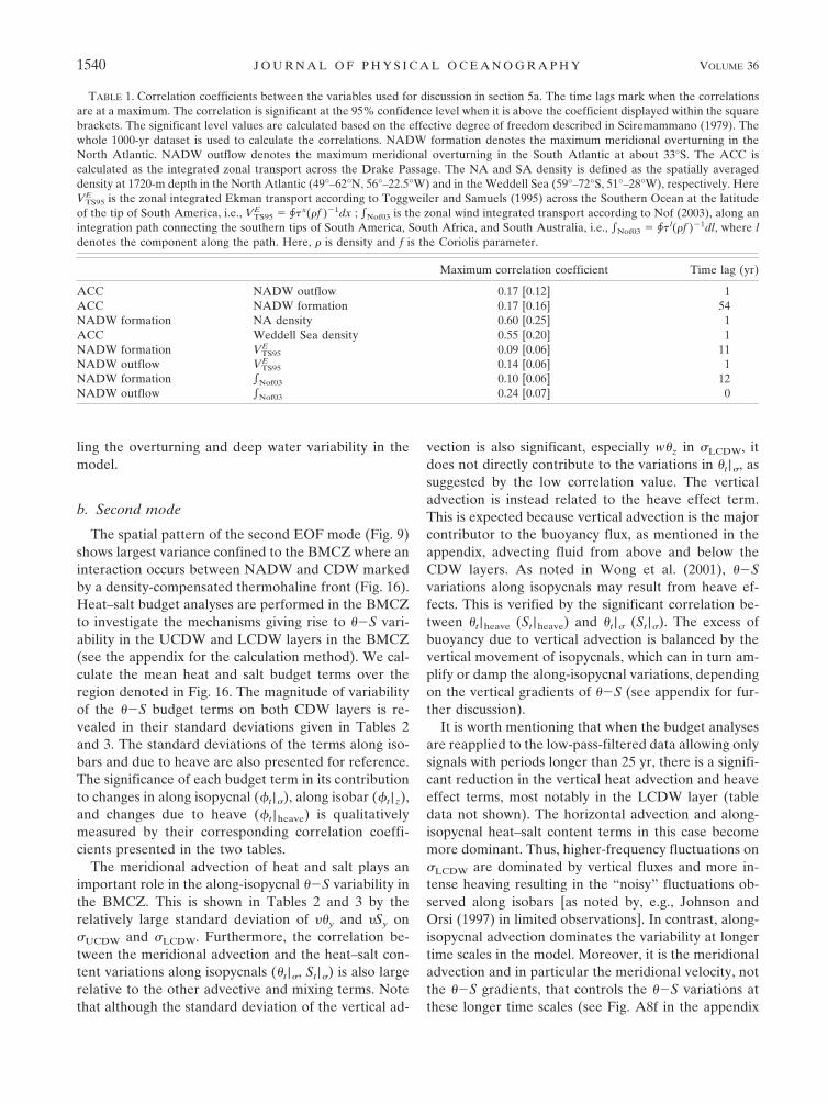
TABLE 1. Correlation coefficients between the variables used for discussion in section 5a. The time lags mark when the correlationsare at a maximum. The correlation is significant at the 95% confidence level when it is above the coefficient displayed within the squarebrackets. The significant level values are calculated based on the effective degree of freedom described in Sciremammano (1979). Thewhole 1000-yr dataset is used to calculate the correlations. NADW formation denotes the maximum meridional overturning in theNorth Atlantic. NADW outflow denotes the maximum meridional overturning in the South Atlantic at about 33°S. The ACC iscalculated as the integrated zonal transport across the Drake Passage. The NA and SA density is defined as the spatially averageddensity at 1720-m depth in the North Atlantic (49°–62°N, 56°–22.5°W) and in the Weddell Sea (59°–72°S, 51°–28°W), respectively. HereVE

TS95 is the zonal integrated Ekman transport according to Toggweiler and Samuels (1995) across the Southern Ocean at the latitudeof the tip of South America, i.e., VE

TS95 � � x(�f )�1dx ; Nof03 is the zonal wind integrated transport according to Nof (2003), along anintegration path connecting the southern tips of South America, South Africa, and South Australia, i.e., Nof03 � � l(�f )�1dl, where ldenotes the component along the path. Here, � is density and f is the Coriolis parameter.

Maximum correlation coefficient Time lag (yr)

ACC NADW outflow 0.17 [0.12] 1ACC NADW formation 0.17 [0.16] 54NADW formation NA density 0.60 [0.25] 1ACC Weddell Sea density 0.55 [0.20] 1NADW formation VE

TS95 0.09 [0.06] 11NADW outflow VE

TS95 0.14 [0.06] 1NADW formation Nof03 0.10 [0.06] 12NADW outflow Nof03 0.24 [0.07] 0


at R1). Therefore, deep ��S variability in the BMCZappears to be controlled by oscillations in both thesouthward DWBC advecting warm–saline NADW, andthe northward Malvinas Current advecting cold–freshCDW.

To explore this further, Fig. 17 presents compositemaps for the �UCDW layer showing velocity anomaliesduring “extreme years” in ��S properties. By extremewe refer to years when the ��S anomalies in theBMCZ are above and below one standard deviationunit, denoted as warm–saline and cold–fresh years, re-spectively. Warm–saline years in the BMCZ are thusconfirmed to occur with an increase in the speed of theDWBC and a coinciding decrease in the speed of theMalvinas Current. The opposite occurs during cold–fresh years. This pattern also exists on �LCDW (figurenot shown). We now denote �DWBC and �MC as theaverage speeds of the DWBC and Malvinas Current,respectively, over the regions shown in Fig. 17a. Thesecurrents fluctuate with ��S in the BMCZ on a widefrequency band, with �DWBC (�MC) and ��S being posi-tively (negatively) correlated with a significant coeffi-cient of �0.4 (�0.4). Spectral analyses between �DWBC

and �MC are shown in Fig. 18 for frequencies lower than0.05 cpy (i.e., �20 yr period); we omit higher frequen-cies as the cross spectra show little energy for shortperiod variability (Fig. 18b). Coherence spectra in Fig.18a suggest that there is significant coherence (above95% confidence level) mainly at periods longer than 50yr. Note also that the DWBC and the Malvinas Currentare shown in Fig. 18c to be approximately out of phaseover multidecadal time scales. This implies that whenthe DWBC strengthens, the Malvinas Current weakens,and vice versa. In summary, an interaction between theDWBC and the Malvinas Current gives rise to ��Sfluctuations in the BMCZ on multidecadal to centen-nial time scales via meridional advection of heat andsalt. The anomalous ��S signals created in the BMCZare then advected eastward by the ACC into the SO(see the eastward propagation shown by CEOF2 in Fig.11).

c. Third mode

The third mode accounts for a small proportion ofthe total variance, and some degree of “mixing” withhigher modes is likely to occur (see section 4c). Thus,we only briefly comment on the possible mechanisms atplay. The spatial pattern of the third EOF mode of�UCDW (Fig. 9) suggests variability sourced in the SouthPacific. Heat–salt budget analyses presented in the ap-pendix suggest zonal heat–salt advective fluxes domi-nate in this region. Oceanic mixing also likely plays arole in distributing the signal into the interior of the

FIG. 16. Spatial thermohaline variation of (a) total density, (b)temperature component, and (c) salinity component at 1720-mdepth. The total density is derived from the linearized equation ofstate � � �r [1 � �(� � �r) � �(S � Sr)], where the subscript rdenotes a reference value. Dashed (solid) contour indicates nega-tive (positive) density anomaly. The boxed region marks the BMCZ.


Indian and Pacific Oceans, particularly along �UCDW

from AAIW sources. The difference between the struc-ture of mode 3 in the UCDW and LCDW layers sug-gests a detectable influence from the AAIW layerabove [AAIW variability in the model has been pre-sented in Santoso and England (2004)]. It should benoted that the analyses of Santoso and England (2004)are based on data filtered for periods higher than 200yr. A low-frequency wavenumber-0 pattern of AAIWvariability accounts for 24% of the total variance of theunfiltered AAIW ��S. This variability mode appearsto be strongest in the AAIW outcrop region south ofAustralia, spreading into the ocean interior over dec-adal to multicentennial periodicities (figure not shown).A coherence analysis between this AAIW ��S modeand PC3 reveals some significant coherence at decadalto centennial time scales, with the cross spectrum be-tween the two time series highest at 250-yr period (fig-ure not shown). Thus, an AAIW signal is likely trans-mitted to the UCDW layer (via diapycnal mixing; seeFigs. A7e,f in the appendix) and then advected east-

ward and northward into the Indian and Pacific basins(see CEOF3 maps in Fig. 11). This appears consistentwith the decadal cooling and freshening found in theAAIW core, which extends to UCDW as documentedby Johnson and Orsi (1997) in the South Pacific. Themechanism controlling the EOF3 mode in the �LCDW

remains unexplained.

6. Summary and conclusions

The spatial distribution of CDW properties and theNADW extent in the SO was shown to be realisticallysimulated in the CSIRO climate model. The CDW wa-ter mass was divided into an upper and lower isopycnallayer, denoted as �UCDW and �LCDW, respectively. Thevariability of CDW ��S is large in the Atlantic alongthe western boundary and decreases gradually eastwardinto the SO. A high ��S variability is confined to theBMCZ. Zonal and meridional advection determinesthe propagation of anomalies along the isopycnal lay-ers, together with the damping effect of mixing. Heav-

TABLE 3. Same as in Table 2 but for the salt budget terms in the BMCZ. Refer to Eq. (A4) for the salt budget equation analyzed.

Budget termsStd dev

(�10�11 psu s�1)

�UCDW

Std dev(�10�11 psu s�1)

�LCDW

Correlation coefficients Correlation coefficients

St | � St|z St | heave St | � St | z St | heave

St | � 3.20 1 0.85 0.28 1.92 1 0.92 �0.34St | z 3.19 0.85 1 �0.26 2.40 0.92 1 �0.68St | heave 1.37 0.28 �0.26 1 1.11 �0.33 �0.68 1uSx 2.81 �0.31 �0.33 0.02 1.48 �0.37 �0.31 0.05�Sy 2.98 �0.63 �0.61 �0.04 1.82 �0.58 �0.50 0.12wSz 1.29 0.17 �0.10 0.49 0.83 �0.17 �0.37 0.56S�mix 2.06 0.09 �0.04 0.25 1.29 0.06 0.10 �0.13

TABLE 2. Standard deviations (std dev) of heat budget terms and correlation coefficients for all terms vs heat content averaged overthe BMCZ (36.6°–46.2°S, 28°–45°W; see Fig. 16 for the location). The values are presented for both �UCDW and �LCDW in the left andright portions, respectively. Correlation coefficients are shown for 1000 yr of model data. The correlation values are significant above�0.06–0.12 at the 95% significance level. The significant level values vary slightly across each analysis because of varying effectivedegrees of freedom (Sciremammano 1979). The std devs are calculated for each grid box before spatial averaging. Correlationcoefficients are calculated using the spatially averaged variables. Refer to Eq. (A3) for the heat budget equation. The highest std devand correlation values for the advective terms are highlighted in boldface.

Budget termsStd dev

(�10�10°C s�1)

�UCDW

Std dev(�10�10°C s�1)

�LCDW

Correlation coefficients Correlation coefficients

�t | � �t | z �t | heave �t | � �t | z �t | heave

�t | � 1.73 1 0.93 �0.50 1.09 1 0.73 �0.53�t | z 2.28 0.93 1 �0.78 2.25 0.73 1 �0.90�t | heave 1.12 �0.50 �0.78 1 1.74 �0.35 �0.90 1u�x 1.55 �0.31 �0.23 0.03 0.85 �0.37 �0.22 0.06��y 1.60 �0.63 �0.54 �0.22 1.02 �0.59 �0.37 0.13w�z 1.03 �0.17 �0.34 0.53 1.45 �0.14 �0.48 0.57��mix 1.22 0.09 0.15 �0.20 0.73 0.06 0.13 �0.14


ing of isopycnal surfaces driven by variations in � be-comes large in the SO because of stronger vertical ad-vection, giving rise to noisy ��S fluctuations whenviewed along isobars. This spatial pattern of variabilityappears consistent with recently documented observeddecadal ��S variations in CDW.

The spatial structure of ��S variability in the CDWlayers was decomposed via EOF analyses into threedominant variability modes explaining 68% of the totalvariance in �UCDW and 82% in �LCDW (Fig. 9). The firstmode shows significant spatial scale ��S variability ex-tending at its largest magnitude from the SA and de-creasing gradually as it is advected eastward into theSO. This first mode oscillates on multicentennial timescales with �330 yr periodicity, corresponding to aquarter-cycle of �80 yr for anomalies to transit fromthe North to South Atlantic via the DWBC to join theACC. There appears to be an interhemispheric telecon-nection in the generation of the first mode of CDW

FIG. 17. Velocity vectors for (a) the mean circulation, (b) compos-ite map of current velocity anomaly on �UCDW defined for extremewarm–saline years, and (c) cold–fresh years. The extreme events aredefined as those above (below) 1 std dev unit for the warm–saline(cold–fresh) years. The dashed box in (a) indicates the location ofthe BMCZ. Solid boxes in (a) indicate the regions defined for aver-aged values of the DWBC meridional velocity (�DWBC) and themeridional component of the Malvinas Current (�MC).

FIG. 18. Spectral analyses for the meridional components of theDWBC (�DWBC) and the Malvinas Current (�MC). Shown are (a)the coherence spectra, (b) the cross spectra, and (c) the phase forthe �UCDW (solid curve) and �LCDW (dash–dot curve).


variability in the model. During years of high (low)NADW formation, positive (negative) salinity anoma-lies propagate southward along the deep water layer inthe Atlantic, followed by northward-propagating nega-tive (positive) salinity anomalies at the intermediatedepths in the SA. This salinity anomaly propagation hasalso been observed on similar time scales in the Ham-burg large-scale geostrophic OGCM (Mikolajewicz andMaier-Reimer 1990; Pierce et al. 1995; Osborn 1997).NADW formation is mainly driven by buoyancy forcingon these time scales, with our analyses suggesting onlya weak connection between NADW formation and SHwinds (as originally proposed by Toggweiler and Sam-uels 1995). On the other hand, the SH winds wereshown to have a more direct influence on NADW out-flow into the SO. In particular, following the proposedcalculation of Nof (2003) we found a significant corre-lation between SH winds and NADW outflow.

The second mode of CDW variability is sourced inthe BMCZ before being advected eastward by theACC. It is characterized by interdecadal to centennialtime scales of variability, and driven by an interactionbetween the southward DWBC and the northwardMalvinas Current via meridional advective fluxes.When the DWBC accelerates, the Malvinas Currentweakens, resulting in local warming and salination ofCDW. The converse occurs during the cooling andfreshening scenario. A similar mechanism has been ob-served in the upper ocean of the BMCZ on seasonal–annual time scales (Garzoli and Giulivi 1994) and onmultidecadal time scales (Wainer and Venegas 2002),under the influence of local atmospheric variability. Asfar as we are aware there have been no studies of dec-adal deep water variability in the BMCZ. Our modelresults suggest that this region is a hub of CDW vari-ability, and thus likely to be a difficult region to analyzewith only sparse data coverage.

The third mode of CDW variability showed fluctua-tions of UCDW sourced in the South Pacific. In theLCDW layer, there was no such source of variability inthis region. Thus, AAIW is the most likely source ofthis mode of UCDW variability. Vertical mixing andzonal advection were seen to play an important role inthe transmission and propagation of the AAIW vari-ability into the UCDW layer.

In summary, this study finds that a large componentof CDW variability originates from the NA via outflow-ing NADW. Significant variability also arises becauseof fluctuations in the SO circulation, particularly in theBMCZ. To a lesser extent, AAIW variability also con-tributes to the upper-layer variability of CDW. Futureresearch should be carried out using sensitivity experi-ments and observations to understand the evolution of

this deep water mass over a range of time scales andunder different climate change scenarios. This is impor-tant because CDW is a key component of the globalocean thermohaline circulation, interacting with our cli-mate on long time scales and influencing the ocean’slarge-scale redistribution of heat, salt, carbon, and nu-trients.

Acknowledgments. The authors gratefully acknowl-edge Mark Collier for preparing the model data outputand Barrie Hunt for allowing us access to the 10 000-yrclimate model simulations. We thank David Jackett forthe equation of state routines and two anonymous re-viewers for their constructive comments and sugges-tions. Discussions with You Yuzhu, Chris Aiken, andTrevor McDougall are also acknowledged. This re-search was supported by the Australian ResearchCouncil and Australian Antarctic Science Program andthe Antarctic Climate and Ecosystems Cooperative Re-search Centre (ACE CRC).

APPENDIX

Along-Isobar, Isopycnal, and Heave Componentsof ��S Changes

a. Heat and salt budget analysis

This section described the heat–salt budget calcula-tion along isopycnal layers. Referring to Fig. A1, wefirst consider a volume of fluid with property � (i.e., �or S) at year t � n � 1 along an isopycnal surface atdepth z � h|t�n�1, where we use | t�n

� and | t�nz notations

hereinafter to denote along-isopycnal and along-isobarprocesses, respectively, at year t � n. As changes inheat and salt fluxes occur at year t � n � 1, the propertyof the fluid volume at z � h|t�n�1 (�| t�n�1

� ) changes to�| t�n

z in the following year at that depth level, while theisopycnal surface has been vertically displaced. Theheat and salt storage rates at a fixed depth at time t �n can be approximately expressed as a function of theadvection and total mixing terms:

�t |zt�n �

� |zt�n � �z

t�n�1

�t

� �u � �� | t�n�1 � ��mix | t�n�1,

�A1�

where �t � 1 yr, the subscript t denotes the differen-tiation with respect to time, and � denotes the spatialgradient operator.


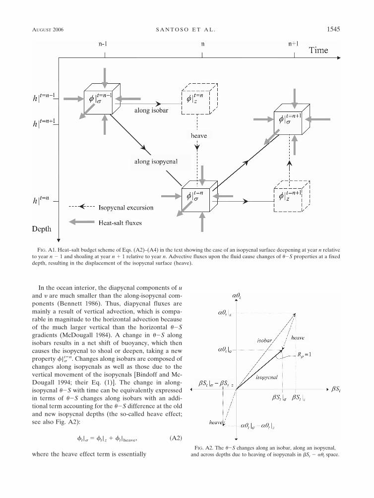
In the ocean interior, the diapycnal components of uand � are much smaller than the along-isopycnal com-ponents (Bennett 1986). Thus, diapycnal fluxes aremainly a result of vertical advection, which is compa-rable in magnitude to the horizontal advection becauseof the much larger vertical than the horizontal ��Sgradients (McDougall 1984). A change in ��S alongisobars results in a net shift of buoyancy, which thencauses the isopycnal to shoal or deepen, taking a newproperty � | t�n

� . Changes along isobars are composed ofchanges along isopycnals as well as those due to thevertical movement of the isopycnals [Bindoff and Mc-Dougall 1994; their Eq. (1)]. The change in along-isopycnal ��S with time can be equivalently expressedin terms of ��S changes along isobars with an addi-tional term accounting for the ��S difference at the oldand new isopycnal depths (the so-called heave effect;see also Fig. A2):

�t |� � �t |z � �t |heave, �A2�

where the heave effect term is essentiallyFIG. A2. The ��S changes along an isobar, along an isopycnal,

and across depths due to heaving of isopycnals in �St � ��t space.

FIG. A1. Heat–salt budget scheme of Eqs. (A2)–(A4) in the text showing the case of an isopycnal surface deepening at year n relativeto year n � 1 and shoaling at year n � 1 relative to year n. Advective fluxes upon the fluid cause changes of ��S properties at a fixeddepth, resulting in the displacement of the isopycnal surface (heave).


�t |heave � �h | t�n � h | t�n�1

�t �� |�t�n � � |z

t�n

h | t�n � h | t�n�1�.

Using the equations above, the heat and salt storagerates along isopycnals can be written as

�t |� � ��u�x � ��y � w�z� � ��mix � �t |heave

�A3�

and

St |� � ��uSx � �Sy � wSz� � S�mix � St |heave,

�A4�

where the first term of the right-hand side of Eqs. (A3)and (A4) shows the zonal, meridional, and verticalcomponents of the advective flux. The heave term isnecessary to balance the total advective flux, which alsocontains diapycnal components [cf. McDougall 1984;his Eqs. (1) and (2)]. The same calculation as givenabove is repeated for each consecutive year over the1000-yr model integration.

b. Visualizing the heat–salt content terms

Inspired by the work of Bindoff and McDougall(1994), we present here a simple method to visualizethe heat–salt storage rate, or content terms in Eq. (A2)over the whole 1000 yr of the model run. We first con-sider the linearized equation of state and its time de-rivative:

� � �r �1 � �� r� � �S � Sr�� and �A5�

�r�1�t � ��t � St, �A6�

where �r is density at a reference pressure pr (i.e., �r �1036.75 kg m�3 for �UCDW and 1036.85 kg m�3 for�LCDW at pr � 2000 db); �r and Sr are the referencepotential temperature and salinity for the correspond-

FIG. A3. Quadrants defined by the Turner angle (Tu) whereheat–salt storage changes are shown in ��t � �St space. The quad-rants bound by the lines R� � 1 and R� � �1 indicate which of �and S dominates in the resulting density changes. The line R� � 1indicates perfect density compensating variations of ��S. The lineR� � �1 indicates density instability as ��S changes are out ofphase.

FIG. A4. Along-isopycnal warming and salination case in �St � ��t space at R1–R4 along �UCDW over the 1000-yr model data in termsof Tu (refer to Fig. A3). The along-isobar (black dots) and along-isopycnal (gray crosses) variations are presented together in the toprow. The corresponding heave effect variations are displayed in the bottom row. The locations of R1–R4 are shown in Fig. A6 (alsoFig. 4c). The abbreviations WF, WS, CS, and CF indicate the signs of ��S change, corresponding to warming–freshening, warming–salination, cooling–salination, and cooling–freshening, respectively.


ing layer; and � and � are the thermal and haline ex-pansion coefficients at pr, respectively. The influence ofheat and salt changes on density is inferred by Eq. (A6),and thus their proportional contribution to changes indensity can be deduced by the stability ratio:

R� ��t

St. �A7�

For example, when warming has a more prominent ef-fect that salination in altering density, R� will be greaterthan 1. This scenario can be visualized by plotting ��t �R��St (Fig. A2). Note that R� is 1 for along-isopycnal��S fluctuations as there is no change in density [i.e.,�t |� is always 0; see Eq. (A8)]. Furthermore, it can beshown from the equations above and Eq. (A2) that

�t |� � �t |z � �t |heave, �A8�

which implies that density fluctuations along isobars areaccompanied by vertical excursions of the isopycnalsurface such that density is conserved (i.e., �t |� � 0;marked by R� � 1 in Fig. A2).

Although the stability ratio R� reveals the competingcontribution of heat and salt changes on density, it doesnot provide information on the sign of the ��S change(i.e., whether the change is related to warming–salina-tion, or warming–freshening, and so on). For this pur-pose, we use the Turner angle (Tu):

Tu � tan�1�R��, �A9�

first described in Ruddick (1983) for diagnosing staticstability of the water column due to mixing and stirring(see also, e.g., May and Kelley 2002). Here Tu is used in

terms of density stability as a result of � � S temporalevolution. The convention of Tu is shown in Fig. A3for defining stability quadrants. Density increases occurin the quadrants below the line R� � 1; density de-creases occur above this line (the quadrants are boundby the lines R� � �1). Note that Tu � 90° and Tu ��90° (R� � ��) denote pure warming and pure cool-ing, and Tu � 0° and Tu � �180° (R� � 0) denote puresalination and pure freshening, respectively. The sub-scripts � and S in each sector indicate the dominance ofeither heat or salt on buoyancy. For example, if ��Schange lies in the WS� sector, this denotes that thewarming–salination that has occurred is dominated bythe change in temperature.

The focus of the heat–salt budget analyses describedin section a is on the along-isopycnal component. Fur-thermore, since the sign of the heat and salt contentterms along isopycnals are either both positive (warm-ing–salination) or both negative (cooling–freshening),the visualization can be presented in terms of either ofthese two cases. Figure A4 presents the plot of the

FIG. A5. The same as Fig. A4 but for �LCDW.

FIG. A6. Transect across the Southern Ocean where the heat–salt budget analyses of Figs. A7 and A8 are conducted. The loca-tions labeled R1–R4 are taken as examples for discussion andcorrespond to R1–R4 used throughout the text and shown in Figs.4c and 5c.


heat–salt content terms that correspond to warming–salination along the isopycnals for �UCDW at R1–R4(see Fig. A6 for R1–R4 locations). The plots for �LCDW

are presented in Fig. A5. The along-isobar and along-isopycnal components are marked with dots and crossesrespectively in the top row of the figures, and the cor-responding heave effect component in the bottom row.It can be noted that the along-isopycnal component liesalong R� � 1 at Tu � 45°. Of course, the along-isobarand heave effect components can occur outside the WSquadrant even when warming–salination occurs along-isopycnal (e.g., Fig. A2). Together with the heat–saltbudget analyses, this visualization method aids with theinterpretation of the processes giving rise to the ��Svariability structure shown in Fig. 6.

c. Heat–salt budget across the ACC

The heat–salt budget analyses are presented along atransect on �UCDW of the SO, passing through R1–R4(Fig. A6). The standard deviations of the heat–salt con-tent and advection terms along the transect are pre-sented in Fig. A7 [refer to Eqs. (A3), (A4) for thebudget equations]. The size of the along-isopycnalvariations at R1 (southwestern Atlantic, near theBMCZ) is much larger than that of the heave varia-tions, indicating that only small density variations occuralong isobars (Figs. A7a,b). This is confirmed in Fig. A4showing variations clustered around Tu � 45° in theWS quadrant. Thus, horizontal advection is likely toplay a dominant role at R1, since horizontal advection

FIG. A7. Std devs of (a) heat content terms, (b) salt content terms, (c) heat advection terms, (d) salt advection terms, (e) heatmixing terms, and (f) salt mixing terms.


mainly moves fluid along isopycnals. In fact, the me-ridional advection is shown in Figs. A7c,d to be thedominant term in the SA and is connected to the along-isopycnal ��S variations, as suggested by the signifi-cant correlation in Figs. A8a,b. The influence of themeridional advection decreases into the Indian and Pa-cific, while the contribution of the zonal advection onthe along-isopycnal heat–salt variations becomes moreprominent (Figs. A8a,b).

As the magnitude of the along-isopycnal variationsbecomes smaller relative to the heave variations atR2–R4 (Indian–Pacific), the variations along isobarsare seen to be distributed outside the WS quadrant,indicating greater variations in buoyancy (Fig. A4). The

vertical advection term is dominant at these locations(Figs. A7c,d) injecting fluid of different densities intothe CDW layer. Referring to Fig. A4, the variationspread on �UCDW at these three locations are seen inthe WF and CS quadrants. This can be explained by the��S vertical structure in Fig. A9 in which vertical fluxesinject warmer and fresher water from above, and coolerand more saline water from below, into the �UCDW

surface (refer to Fig. 3 for the definition of the �UCDW

surface). In the process, the vertical displacement of�UCDW tends to damp the excessive heat content andamplifies the degraded salt content due to the verticalinjection. This can be seen in the correlations betweenthe along-isopycnal heat–salt content terms and the

FIG. A8. Correlation coefficients for (a) heat advection terms vs �t | �, (b) salt advection terms vs St | �, (c) �t | heave vs w�z and �t | �, (d)St | heave vs wSz and St | �, (e) zonal heat advection term (u�x) vs �x and u, and (f) meridional heat advection term (��y) vs �y and �.Correlation coefficients that are not significant above the 95% confidence level are not displayed.


heave effect terms (Figs. A8c,d). Thus, the heave effectmodulates the influence of vertical fluxes such that thealong-isopycnal heat–salt contents are preserved. Theeffect of heave on the along-isopycnal variations wouldbe more significant when the vertical ��S gradients aredensity compensating with large vertical salinity gradi-ent such that S drives the buoyancy perturbation (seealso Yeager and Large 2004). Although the vertical��S gradients are of the same sign in the LCDW layer(Fig. A9), � is more prominent than S on buoyancy(Fig. A4); thus, heaving likely acts to damp the verticalfluxes and contributes little to along-isopycnal variabil-ity. The vertical ��S gradients in the UCDW layer alsotends to inhibit the effect of heaving to introducechanges along isopycnals.

The large along-isopycnal heat–salt content varia-tions at 170°E–160°W (Figs. A7a,b) coincide with thelarge ��S variance seen in the South Pacific in theEOF1 and 3 modes for �UCDW (Fig. 9). In this region,the standard deviations in the zonal and vertical advec-tive fluxes are large (Figs. A7c,d). However, only thezonal advection term is significantly correlated to theheat–salt content terms (Figs. A8a,b). The ��S vari-ability in this region is thus controlled by the zonaladvective flux driven by ��S gradients rather than theACC (Fig. A8e; figure not shown for S). Furthermore,since this large variability in the South Pacific does notextend down to the LCDW layer (Fig. 7), it is likely thatthe source of this variability is from the AAIW layer viadiapycnal mixing. Note that Figs. A7e,f show large mix-ing variability in the South Pacific as well as at R1 in theBMCZ. The mixing variability in the South Pacific is inthe vertical, whereas it is meridional at the BMCZ. Thisis consistent with the above physical interpretations.

REFERENCES

Arbic, B. K., and W. B. Owens, 2001: Climatic warming of Atlan-tic intermediate waters. J. Climate, 14, 4091–4108.

Bennett, S. L., 1986: The relationship between vertical, diapycnal,and isopycnal velocity and mixing in the ocean general cir-culation. J. Phys. Oceanogr., 16, 167–174.

Bianchi, A. A., C. F. Giulivi, and A. R. Piola, 1993: Mixing in theBrazil–Malvinas Confluence. Deep-Sea Res. I, 40, 1345–1358.

Bindoff, N. L., and T. J. McDougall, 1994: Diagnosing climatechange and ocean ventilation using hydrographic data. J.Phys. Oceanogr., 24, 1137–1152.

——, and ——, 2000: Decadal changes along an Indian Oceansection at 32°S and their interpretation. J. Phys. Oceanogr.,30, 1207–1222.

Callahan, J. E., 1972: The structure and circulation of Deep Waterin the Antarctic. Deep-Sea Res., 19, 563–575.

Charles, C. D., and R. G. Fairbanks, 1992: Evidence from South-ern Ocean sediments for the effect of North Atlantic deep-water flux on climate. Nature, 355, 416–419.

Cox, M. D., 1984: A primitive equation, three-dimensional modelof the ocean. GFDL Ocean Group Tech. Rep. 1, GFDL,Princeton University, Princeton, NJ, 141 pp.

Dickson, R. R., and J. Brown, 1994: The production of NorthAtlantic Deep Water: Sources, rates, and pathways. J. Geo-phys. Res., 99, 12 319–12 341.

Döös, K., and A. Coward, 1997: The Southern Ocean as the majorupwelling zone of North Atlantic Deep Water. InternationalWOCE Newsletter, No. 27, WOCE International Project Of-fice, Southampton, United Kingdom, 3–4.

England, M. H., and A. C. Hirst, 1997: Chlorofluorocarbon up-take in a World Ocean model. 2. Sensitivity to surface ther-mohaline forcing and subsurface mixing parameterizations. J.Geophys. Res., 102, 15 709–15 731.

——, and G. Holloway, 1998: Simulations of CFC content andwater mass age in the deep North Atlantic. J. Geophys. Res.,103, 15 885–15 901.

——, and S. Rahmstorf, 1999: Sensitivity of ventilation rates andradiocarbon uptake to subgrid-scale mixing in ocean models.J. Phys. Oceanogr., 29, 2802–2827.

Frank, M., N. Whiteley, S. Kasten, J. R. Hein, and K. O’Nions,2002: North Atlantic Deep Water export to the SouthernOcean over the past 14 Myr: Evidence from Nd and Pb iso-topes in ferromanganese crusts. Paleoceanography, 17, 1022,doi:10.1029/2000PA000606.

García, M. A., I. Bladé, A. Cruzado, Z. Velásquez, H. García, J.Puigdefäbregas, and J. Sospedra, 2002: Observed variabilityof water properties and transports on the World Ocean Cir-culation Experiment SR1b section across the Antarctic Cir-cumpolar Current. J. Geophys. Res., 107, 3162, doi:10.1029/2000JC000277.

Garzoli, S. L., and C. Giulivi, 1994: What forces the variability ofthe southwestern Atlantic boundary currents? Deep-Sea Res.I, 41, 1527–1550.

Gent, P. R., and J. C. McWilliams, 1990: Isopycnal mixing inocean circulation models. J. Phys. Oceanogr., 20, 150–155.

——, J. Willebrand, T. J. McDougall, and J. C. McWilliams, 1995:Parameterizing eddy-induced tracer transports in ocean cir-culation models. J. Phys. Oceanogr., 25, 463–474.

Georgi, D. T., 1981: On the relationship between the large-scaleproperty variations and fine structure in the CircumpolarDeep Water. J. Geophys. Res., 86, 6556–6566.

Goodman, P. J., 1998: The role of North Atlantic Deep Water

FIG. A9. �–S vertical profiles at R1–R4. The locations of R1–R4are shown in Fig. A6.


formation in an OGCM’s ventilation and thermohaline cir-culation. J. Phys. Oceanogr., 28, 1759–1785.

——, 2001: Thermohaline adjustment and advection in anOGCM. J. Phys. Oceanogr., 31, 1477–1497.

Gordon, A. L., 1989: Brazil–Malvinas Confluence—1984. Deep-Sea Res., 36, 359–384.

Gordon, H. B., and S. P. O’Farrell, 1997: Transient climate changein the CSIRO coupled model with dynamic sea ice. Mon.Wea. Rev., 125, 875–907.

Hirst, A. C., and T. J. McDougall, 1996: Deep-water propertiesand surface buoyancy flux as simulated by a z-coordinatemodel including eddy-induced advection. J. Phys. Oceanogr.,26, 1320–1343.

——, S. P. O’Farrell, and H. B. Gordon, 2000: Comparison of acoupled ocean–atmosphere model with and without oceaniceddy-induced advection. Part I: Ocean spinup and controlintegrations. J. Climate, 13, 139–163.

Horel, J. D., 1984: Complex principal component analysis: Theoryand examples. J. Climate Appl. Meteor., 23, 1660–1673.

Johnson, G. C., and A. H. Orsi, 1997: Southwest Pacific Oceanwater-mass changes between 1968/69 and 1990/91. J. Climate,10, 306–316.

Kamenkovich, I. V., and E. S. Sarachik, 2004: Mechanisms con-trolling the sensitivity of the Atlantic thermohaline circula-tion to the parameterization of eddy transports in oceanGCMs. J. Phys. Oceanogr., 34, 1628–1647.

Kowalczyk, E. A., J. R. Garratt, and P. B. Krummel, 1994: Imple-mentation of a soil canopy scheme into the CSIRO GCM—Regional aspects of the model response. CSIRO Division ofAtmospheric Research, Tech. Paper 32, 59 pp. [Availablefrom CSIRO Atmospheric Research, PMB1, Aspendale,VIC 3195, Australia.]

Larqué, L., K. Maamaatuaiahutapu, and V. Garçon, 1997: On theintermediate and deep water flows in the South AtlanticOcean. J. Geophys. Res., 102, 12 425–12 440.

Levitus, S., and T. P. Boyer, 1994: Temperature. Vol. 4, WorldOcean Atlas 1994, NOAA Atlas NESDIS 4, 117 pp.

——, R. Burgett, and T. P. Boyer, 1994: Salinity. Vol. 3, WorldOcean Atlas 1994, NOAA Atlas NESDIS 3, 99 pp.

Maamaatuaiahutapu, K., V. C. Garçon, and C. Provost, 1992: Bra-zil–Malvinas Confluence: Water mass composition. J. Geo-phys. Res., 97, 9493–9505.

Mann, M. E., and J. M. Lees, 1996: Robust estimation of back-ground noise and signal detection in climatic time series. Cli-matic Change, 33, 409–445.

Mantyla, A. W., and J. L. Reid, 1983: Abyssal characteristics ofthe World Ocean waters. Deep-Sea Res., 30, 805–833.

——, and ——, 1995: On the origins of deep and bottom waters ofthe Indian Ocean. J. Geophys. Res., 100, 2417–2439.

May, B. D., and D. E. Kelley, 2002: Contrasting the interleaving intwo baroclinic ocean fronts. Dyn. Atmos. Oceans, 36, 23–42.

McDougall, T. J., 1984: The relative roles of diapycnal and iso-pycnal mixing on subsurface water mass conversion. J. Phys.Oceanogr., 14, 1577–1589.

McNeil, B. I., R. J. Matear, and B. Tilbrook, 2001: Does carbon-13track anthropogenic CO2 in the Southern Ocean? GlobalBiogeochem. Cycles, 15, 597–613.

Mémery, L., M. Arhan, X. A. Alvarez-Salgado, M.-J. Messias, H.Mercier, C. G. Castro, and A. F. Rios, 2000: The watermasses along the western boundary of the south and equa-torial Atlantic. Progress in Oceanography, Vol. 47, PergamonPress, 69–98.

Mikolajewicz, U., and E. Maier-Reimer, 1990: Internal secular

variability in an ocean general circulation model. ClimateDyn., 4, 145–156.

Nof, D., 2003: The Southern Ocean’s grip on the northward me-ridional flow. Progress in Oceanography, Vol. 56, PergamonPress, 223–247.

North, G. R., T. L. Bell, R. F. Cahalan, and F. J. Moeng, 1982:Sampling errors in the estimation of empirical orthogonalfunctions. Mon. Wea. Rev., 110, 699–706.

O’Farrell, S. P., 1998: Sensitivity study of a dynamical sea icemodel: The effect of the external stresses and land boundaryconditions on ice thickness distribution. J. Geophys. Res., 103,15 751–15 782.

——, 2002: Use of passive tracers as a diagnostic tool in coupledmodel simulations—Northern Hemisphere. J. Phys. Ocean-ogr., 32, 831–850.

Oke, P. R., and M. H. England, 2004: Oceanic response tochanges in the latitude of the Southern Hemisphere subpolarwesterly winds. J. Climate, 17, 1040–1054.

Osborn, T. J., 1997: Thermohaline oscillations in the LSGOGCM: Propagating anomalies and sensitivity to parameter-izations. J. Phys. Oceanogr., 27, 2233–2255.

Percival, D. B., and A. T. Walden, 1993: Spectral Analysis forPhysical Applications. Cambridge University Press, 583 pp.

Pierce, D. W., T. P. Barnett, and U. Mikolajewicz, 1995: Compet-ing roles of heat and freshwater flux in forcing thermohalineoscillations. J. Phys. Oceanogr., 25, 2046–2064.

Preisendorfer, R. W., 1988: Principal Component Analyses in Me-teorology and Oceanography. Elsevier, 425 pp.

Prézelin, B. B., E. E. Hofmann, C. Mengelt, and J. M. Klinck,2000: The linkage between Upper Circumpolar Deep Water(UCDW) and phytoplankton assemblages on the west Ant-arctic Peninsula continental shelf. J. Mar. Res., 58, 165–202.

Rahmstorf, S., and M. H. England, 1997: Influence of SouthernHemisphere winds on North Atlantic Deep Water flow. J.Phys. Oceanogr., 27, 2040–2054.

Reid, J. L., 1986: On the total geostrophic circulation of the SouthPacific Ocean: Flow patterns, tracers and transports. Progressin Oceanography, Vol. 16, Pergamon Press, 1–61.

——, W. D. Nowlin, and W. C. Patzert, 1977: On the characteris-tics and circulation of the southwestern Atlantic Ocean. J.Phys. Oceanogr., 7, 62–91.

Rintoul, S. R., and M. H. England, 2002: Ekman transport domi-nates local air–sea fluxes in driving variability of SubantarcticMode Water. J. Phys. Oceanogr., 32, 1308–1320.

Ruddick, B., 1983: A practical indicator of the stability of thewater column to double-diffusive activity. Deep-Sea Res., 30,1105–1107.

Santoso, A., and M. H. England, 2004: Antarctic IntermediateWater circulation and variability in a coupled climate model.J. Phys. Oceanogr., 34, 2160–2179.

Schmitz, W. J., Jr., 1995: On the interbasin-scale thermohalinecirculation. Rev. Geophys., 33, 151–173.

Schneider, N., 2000: A decadal spiciness mode in the Tropics.Geophys. Res. Lett., 27, 257–260.

Sciremammano, F., 1979: A suggestion for the presentation ofcorrelations and their significance levels. J. Phys. Oceanogr.,9, 1273–1276.

Sen Gupta, A., and M. H. England, 2004: Evaluation of interiorcirculation in a high resolution global ocean model. Part I:Deep and bottom waters. J. Phys. Oceanogr., 34, 2592–2614.

Shaffer, G., O. Leth, O. Ulloa, J. Bendtsen, G. Daneri, V. Del-larossa, S. Hormazabal, and P.-I. Sehlstedt, 2000: Warming


and circulation change in the eastern South Pacific Ocean.Geophys. Res. Lett., 27, 1247–1250.

Sievers, H. A., and W. D. Nowlin Jr., 1984: The stratification andwater masses at Drake Passage. J. Geophys. Res., 89, 10 459–10 514.

Sigman, D. M., and E. A. Boyle, 2000: Glacial/interglacial varia-tions in atmospheric carbon dioxide. Nature, 407, 859–869.

Simmons, H. L., and I. V. Polyakov, 2004: Restoring and flux ad-justment in simulating variability of an idealized ocean. Geo-phys. Res. Lett., 31, L16301, doi:10.1029/2004GL020197.

Sloyan, B. M., and S. R. Rintoul, 2001: The Southern Ocean limbof the global deep overturning circulation. J. Phys. Ocean-ogr., 31, 143–173.

Smethie, W. M., Jr., R. A. Fine, A. Putzka, and E. P. Jones, 2000:Tracing the flow of North Atlantic Deep Water using chlo-rofluorocarbons. J. Geophys. Res., 105, 14 297–14 323.

Speer, K., E. Guilyardi, and G. Madec, 2000: Southern Oceantransformation in a coupled model with and without eddymass fluxes. Tellus, 52A, 554–565.

Stramma, L., and M. England, 1999: On the water masses andmean circulation of the South Atlantic Ocean. J. Geophys.Res., 104, 20 863–20 883.

Swift, J. H., 1984: The circulation of the Denmark Strait and Ice-land–Scotland overflow waters in the North Atlantic. Deep-Sea Res., 31, 1339–1355.

Talley, L. D., 2003: Shallow, intermediate, and deep overturningcomponents of the global heat budget. J. Phys. Oceanogr., 33,530–560.

——, and M. S. McCartney, 1982: Distribution and circulation ofLabrador Sea Water. J. Phys. Oceanogr., 12, 1189–1205.

Toggweiler, J. R., and B. Samuels, 1995: Effect of Drake Passageon the global thermohaline circulation. Deep-Sea Res. I, 42,477–500.

Tsuchiya, M., L. D. Talley, and M. S. McCartney, 1994: Water-mass distributions in the western South Atlantic: A section

from South Georgia Island (54S) northward across the equa-tor. J. Mar. Res., 52, 55–81.

Wainer, I., and S. A. Venegas, 2002: Multidecadal variability inthe Climate System Model. J. Climate, 15, 1408–1420.

Weaver, A. J., and T. M. C. Hughes, 1992: Stability and variabilityof the thermohaline circulation and its link to climate. TrendsPhys. Oceanogr., 1, 15–69.

Weijer, W., and H. A. Dijkstra, 2003: Multiple oscillatory modesof the global ocean circulation. J. Phys. Oceanogr., 33, 2197–2213.

Whitworth, T., III, B. A. Warren, W. D. Nowlin Jr., S. B. Rutz,R. D. Pillsbury, and M. I. Moore, 1999: On the deep western-boundary current in the southwest Pacific basin. Progress inOceanography, Vol. 43, Pergamon Press, 1–54.

Wijffels, S. E., J. M. Toole, and R. Davis, 2001: Revisiting theSouth Pacific subtropical circulation: A synthesis of WorldOcean Circulation Experiment observations along 32°S. J.Geophys. Res., 106, 19 481–19 513.

Wong, A. P. S., N. L. Bindoff, and J. A. Church, 2001: Freshwaterand heat changes in the North and South Pacific Oceansbetween the 1960s and 1985–94. J. Phys. Oceanogr., 14, 1613–1633.

Wunsch, C., D. Hu, and B. Grant, 1983: Mass, heat, salt andnutrient fluxes in the South Pacific Ocean. J. Phys. Ocean-ogr., 13, 725–753.

Wüst, G., 1935: Schichtung und Zirkulation des AtlantischenOzeans. Das Bodenwasser und die Stratosphäre. Wiss. Ergeb.Dt. Atl. Exp. Meteor., 6, 1–288.

Yeager, S. G., and W. G. Large, 2004: Late-winter generation ofspiciness on subducted isopycnals. J. Phys. Oceanogr., 34,1528–1547.

You, Y.-Z., 2000: Implications of the deep circulation and venti-lation of the Indian Ocean on the renewal mechanism ofNorth Atlantic Deep Water. J. Geophys. Res., 105, 23 895–23 926.


Documents

Circumpolar Deep Water Circulation and Variability in a Coupled …web.science.unsw.edu.au/~matthew/se_2006_CDW.pdf · ability along the CDW layers. The rest of this paper is divided