1

Chi-Square Test

J. Savoy Université de Neuchâtel

C. D. Manning & H. Schütze : Foundations of statistical natural language processing. The MIT Press. Cambridge (MA)

2

Discriminating Features

 How can we characterize / discriminate the distribution of a set of given word types (or other linguistic features) for corpus (or a document or a set of documents) in comparison with another? Compare two works of two different authors

 We can used word tokens, word types, bigrams, trigrams, phrases, POS, or even punctuations

 Used in various context   Parallel word-by-word translation

  Pertinent collocations

3

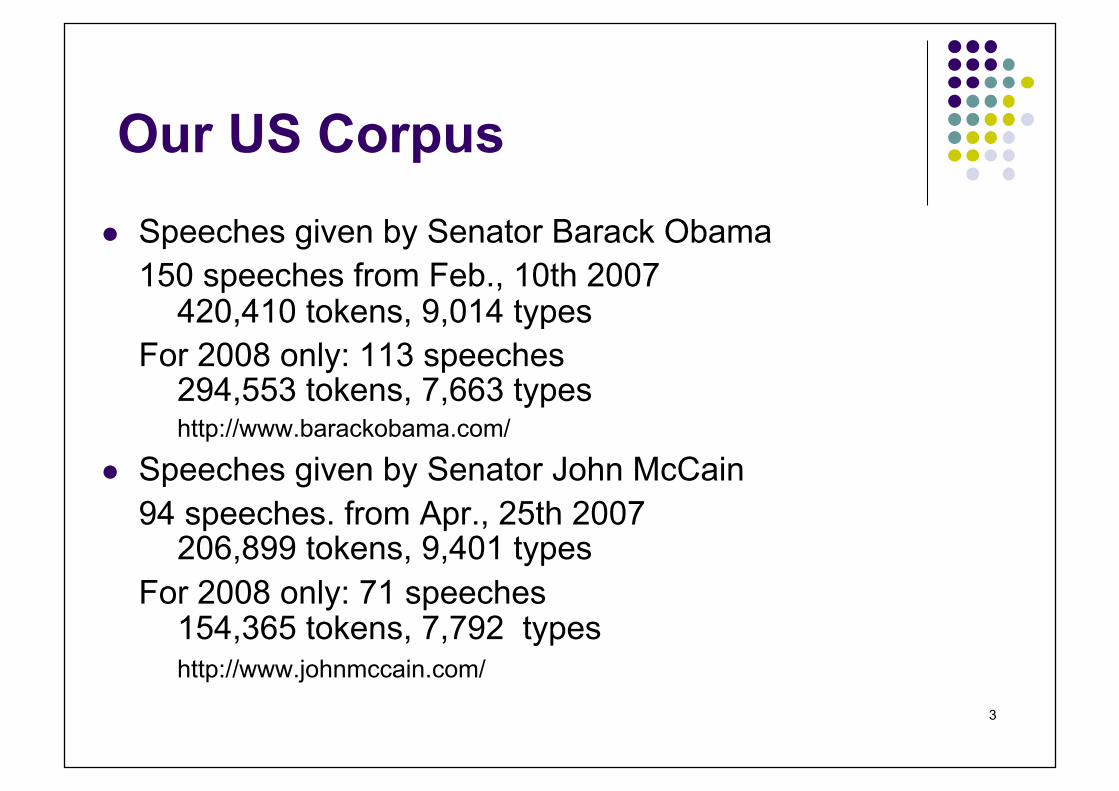
Our US Corpus   Speeches given by Senator Barack Obama

150 speeches from Feb., 10th 2007 420,410 tokens, 9,014 types

For 2008 only: 113 speeches 294,553 tokens, 7,663 types http://www.barackobama.com/

  Speeches given by Senator John McCain 94 speeches. from Apr., 25th 2007

206,899 tokens, 9,401 types For 2008 only: 71 speeches

154,365 tokens, 7,792 types http://www.johnmccain.com/

4

Discriminating Features

 To define whether a given feature (e.g., word, bigram, POS, etc.) is used significantly more often in a given corpus, we may subdivide the whole corpus (C) into two (or more) disjoint parts

 Example: US electoral speeches

5

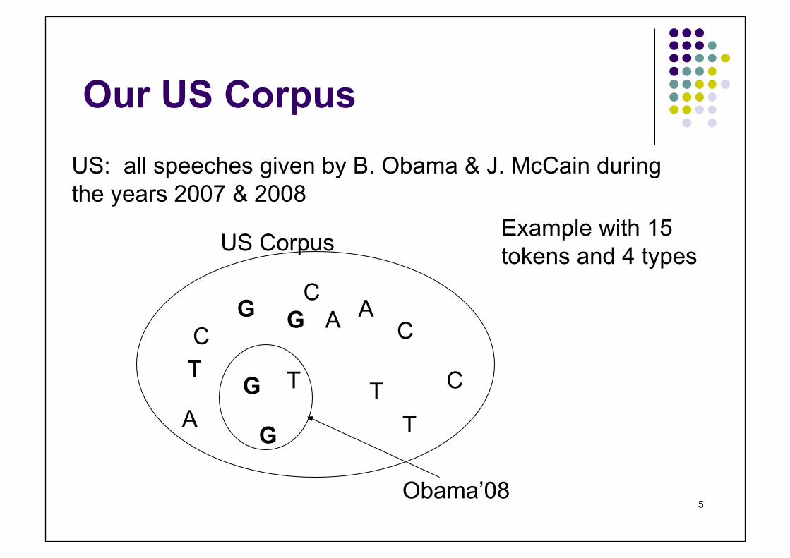
Our US Corpus

US: all speeches given by B. Obama & J. McCain during the years 2007 & 2008

US Corpus

C

T

G

A

G A C

T

T

A C

C

G

T G

Obama’08

Example with 15 tokens and 4 types

6

Contingency Table

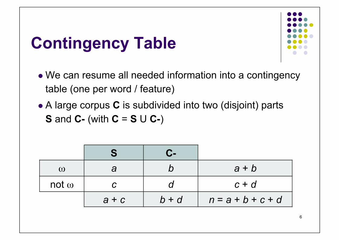
 We can resume all needed information into a contingency table (one per word / feature)

 A large corpus C is subdivided into two (disjoint) parts S and C- (with C = S U C-)

S C- ω a b a + b

not ω c d c + d a + c b + d n = a + b + c + d

7

Contingency Table

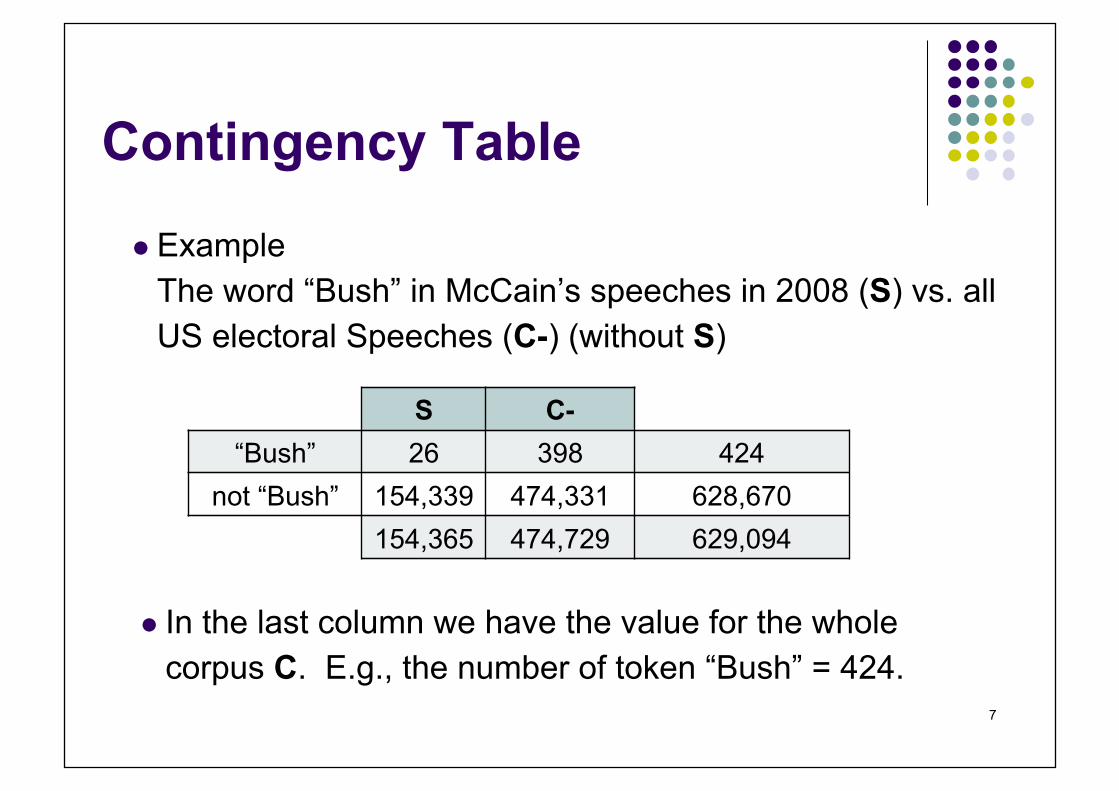
 Example The word “Bush” in McCain’s speeches in 2008 (S) vs. all US electoral Speeches (C-) (without S)

S C- “Bush” 26 398 424

not “Bush” 154,339 474,331 628,670 154,365 474,729 629,094

  In the last column we have the value for the whole corpus C. E.g., the number of token “Bush” = 424.

8

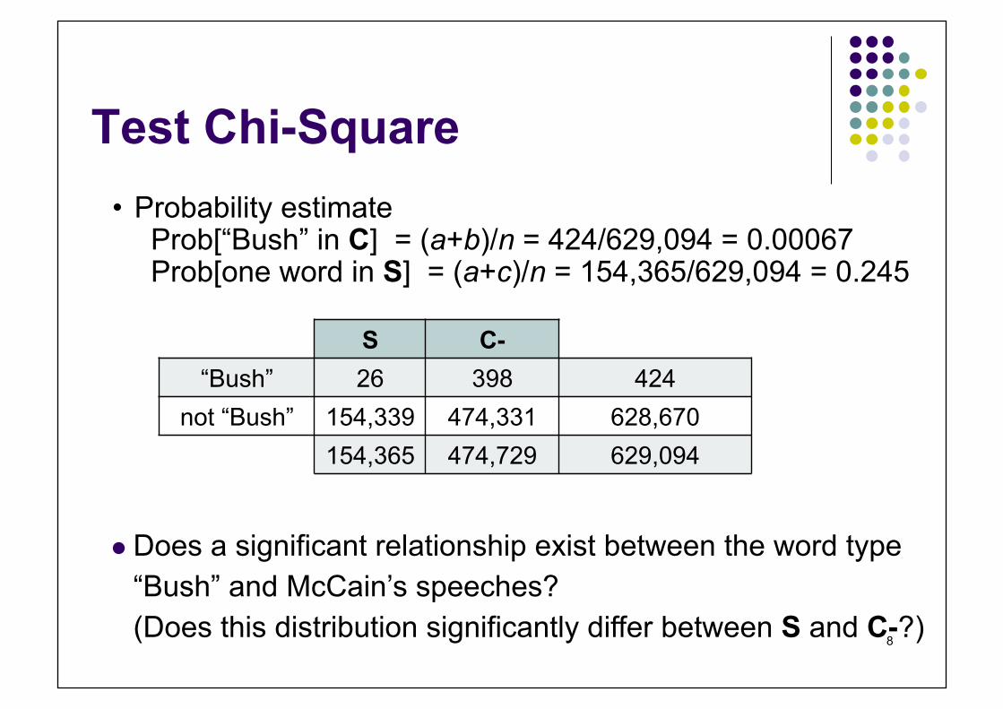
Test Chi-Square •  Probability estimate

Prob[“Bush” in C] = (a+b)/n = 424/629,094 = 0.00067 Prob[one word in S] = (a+c)/n = 154,365/629,094 = 0.245

S C- “Bush” 26 398 424

not “Bush” 154,339 474,331 628,670 154,365 474,729 629,094

 Does a significant relationship exist between the word type “Bush” and McCain’s speeches? (Does this distribution significantly differ between S and C-?)

9

Test Chi-Square  Distribution of four POS tags according to two authors  Does this distribution differ significantly?

Of course, we do not expect having the same values in both columns, but are the differences significant?

Observed McCain’08 Obama’08 Total Percentage NN 33,876 58,550 92,426 41.6%

JJ 10,677 18,517 29,194 13.2% VB 21,927 54,268 76,195 34.3% RB 7,117 17,064 24,181 10.9%

Total 73,597 148,399 221,996 100% Percentage 33.2% 66.8%

10

Test Chi-Square

  Each statistical test is based on a set of assumptions. For the chi-square test (or χ2), we assume (we admit as truth that):

1.  Each sample is a random sample 2.  The samples are mutually independent 3.  Each observation may be categorized into one of the r

categories.

11

Test Chi-Square  First we specify our null hypothesis (H0):

In our example, we assume that the use of one particular POS (for one word) by one author does not imply the use of a given POS (the same or another) by the other author. Under H0, each author will use a similar number of each POS in his speeches (we admit random variations and thus we do not expect exactly the same values). If an author gives more speeches (or longer speeches), of course the number of each POS will increase but proportionally.

12

Test Chi-Square  Second, if the null hypothesis is not true, we must admit the

(unique) alternate hypothesis (H1). In our case, H1 assume that there is a systematic difference in the POS distribution between the two authors. These two hypothesis cannot be true at the same time. Only one of them is true. Which one (according to the available data)?

 Third we compute the expected number of each POS according to each author under this null hypothesis (we do as if the null hypothesis H0 is true)

13

Test Chi-Square For example, McCain produces 73,597 tokens and 41.6% must be nouns. Thus we expect 73,597 x 0.416 = 30,616.4 nouns. This value will be denoted Ei (and the observed value as Oi).

Expected McCain’08 Obama’08 Percentage NN 41.6%

JJ 13.2% VB 50901 34.3% RB 10.9%

Total 73,597 148,399 100%

Percentage 33.2% 66.8%

14

Test Chi-Square  Four we compare the expected and observed numbers and

we compute for each cell (case) (Oi-Ei)2/Ei

Obser ved (Oi) Expec ted (Ei) POS McCain’08 Obama’08 McCain’08 Obama’08 Percentage NN 33876 58550 30616 61734 41.6% JJ 10677 18517 9715 19589 13.2% VB 21927 54268 25244 50901 34.3% RB 7117 17064 8022 16175 10.9%

Total 73,597 148,399 73,597 148,399 100%

For Obama and nouns, we have ((58,550 - 61,734)2 / 61,734) = 164.22. If H0 is (really) true, such differences must be small.

15

Test Chi-Square

 For each cell (case), we compute the square of the difference divided by the expected number. We sum all these values.

McCain’08 Obama’08 NN 347.05 164.22 JJ 95.30 58.63 VB 435.79 222.74 RB 102.11 48.81

Total 980.25 494.39 χ2 = 1474.64

16

Test Chi-Square

 Fifth, the decision The values for our χ2 value is 1474.64 Is this value large? Maybe too large if we admit that H0 is true. How can we “objectively” say “it is too large”? Compare this (computed) value with the maximum value we may expected if H0 is true…

  In fact we must admit an error in our test. Because even rare event has a (very) small probability (that is not null). Thus we must define the value (limit) for which 95% of the observations have a lower value…

17

Test Chi-Square

 We usually prefer specifying that the error α = 5% (significant level 1-α = 95%).

 Second point: The χ2 is a family of distribution (we have more than one such distribution) and to specify which member of this family we need, we specify the number of degree of freedom (dof) which is (r-1).(c-1) This corresponds to the number of rows (r) and the number of columns (c) of our data (ignoring the total and percentage column or row)

18

Test Chi-Square  Limits of the χ2 distribution   In our example, we obtain an

observed value of 1474.64.  The number of dof is

(4-1).(2-1) = 3   If H0 is true, we may expect

having value as large as 7.81 (α = 5%) or 11.3 (α = 1%)

χ2 dof 95% 99%

1 3.84 6.63 2 5.99 9.21 3 7.81 11.3 4 9.49 13.3 5 11.1 15.1 6 12.6 16.8 7 14.1 18.5 8 15.5 20.1 9 16.9 21.7

10 18.3 23.2

19

Test Chi-Square   If H0 is true, we may expect having value as large as 7.81

(with α = 5%) or 11.3 (with α = 1%)  The observed value (1474.64) is larger than this limit (one-

tail test) because we consider (to reject H0) only one tail of the underlying distribution.

 Reject H0 (no difference between the two distributions) and we accept H1 (there is a significant difference)

 Where?

20

Test Chi-Square  The main differences

Obser ved (Oi) Expec ted (Ei) POS McCain’08 Obama’08 McCain’08 Obama’08 NN 33876 58550 30616 61734 JJ 10677 18517 9715 19589 VB 21927 54268 25244 50901 RB 7117 17064 8022 16175

21

Test Chi-Square   We must reject H0 and thus accept H1

(there is a significant difference)  Where?

Obama uses more VB & RB, McCain more NN & JJ  Why?

Discourse analysis & political consideration … Buzzwords of the campaign “Country first: Reform, prosperity, peace” “Yes we can” or “change we believe in”

 Caution: the POS tagger is not perfect!

22

Test Chi-Square (2nd application) •  And for the distribution of the word type “Bush” in

McCain’s speeches in 2008?

Obse rved Expe cted S C- S C-

“Bush” 26 398 104 320 not “Bush” 154,339 474,331 154261 474409

 Computing the difference between the observed and expected values according to the formula

and we obtain χ2 =78.13

23

Test Chi-Square (2nd application)   Is this difference (χ2 =78.13) large? Too large?  Compared with the values in the table of the χ2

under dof = (r-1).(c-1) = 1.1 = 1   If H0 is true, we may expect having value as large as

3.84 (with α = 5%) or 6.63 (with α = 1%)  The computed value χ2 is large than the limit.

The word type “Bush” in McCain’s speeches in 2008 does not follow the distribution of the US electoral speeches. McCain uses less often this name than Obama.

24

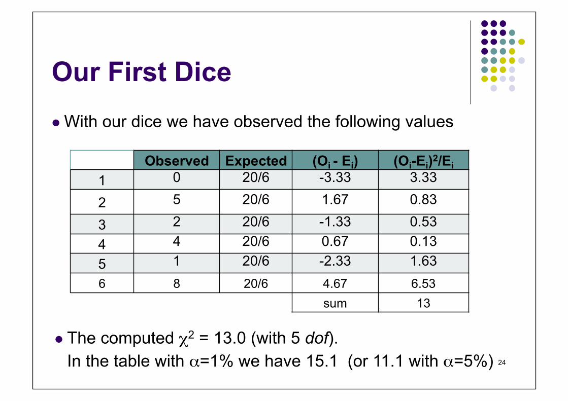
Our First Dice  With our dice we have observed the following values

Observed Expected (Oi - Ei) (Oi-Ei)2/Ei

1 0 20/6 -3.33 3.33

2 5 20/6 1.67 0.83

3 2 20/6 -1.33 0.53 4 4 20/6 0.67 0.13 5 1 20/6 -2.33 1.63 6 8 20/6 4.67 6.53

sum 13

 The computed χ2 = 13.0 (with 5 dof). In the table with α=1% we have 15.1 (or 11.1 with α=5%)

25

Our Second Dice  With our dice we have observed the following values

Observed Expected (Oi - Ei) (Oi-Ei)2/Ei

1 3 20/6 -0.33 0.33

2 5 20/6 1.67 0.83

3 3 20/6 -0.33 0.03 4 5 20/6 1.67 0.83 5 2 20/6 -1.33 0.53 6 2 20/6 1.33 0.53

sum 2.8

 The computed χ2 = 2.8 (with 5 dof). In the table with α=1% we have 15.1 (or 11.1 with α=5%)

26

Limit of the Chi-Square Test

 For each cell, the expected count must be 5 or greater. To avoid multiple cells with low count and thus we can increase (artificially) the χ2 values.

  In studying word frequency, this constraint limits the application of this test to word occurring 5 times or more.

 For a lexical analysis, many word types will not be considered (Zipf’s law)

27

Word Types Distribution  Distribution of word types in the low frequencies classes  Number of word types: 7663 (Obama’08), 7792 (McCain’08)

Frequency Obama’08 McCain’08 1 2573 33.6% 2958 38.0% 2 1042 13.6% 1112 14.3% 3 556 7.3% 641 8.2% 4 446 5.8% 435 5.6% 5 308 4.0% 313 4.0%

For the US corpus, this reduction is from 7,663 to 3,046 (or to 39.8% of the word types) for Obama 2008 and from 7,792 to 2,646 (7792-5146) (or 34%) for McCain 2008.

28

View/Verify the Context

 Finding pertinent (significant) features is the first step  Explaining such phenomena is the second step  Usually it is important to see the context

and again the computer science may help  How?

KWIC + Perl script to specify multiple constraints in selecting words / contexts / sentences

29

KWIC Keyword In Context

 Besides counting linguistic phenomena, computer science may provide other useful tools

  KWIC is such an example  Provide the left and right context (number of words, number

of characters) of a given word (exact spelling)  Can be used to see the context around a term  Example:

Translation of “fort” (JJ) into the English language by “strong” or “powerful” “un fort orage”, “un café fort”, “un médicament fort”

30

Context around “Strong”

31

Context around “Powerful”

32

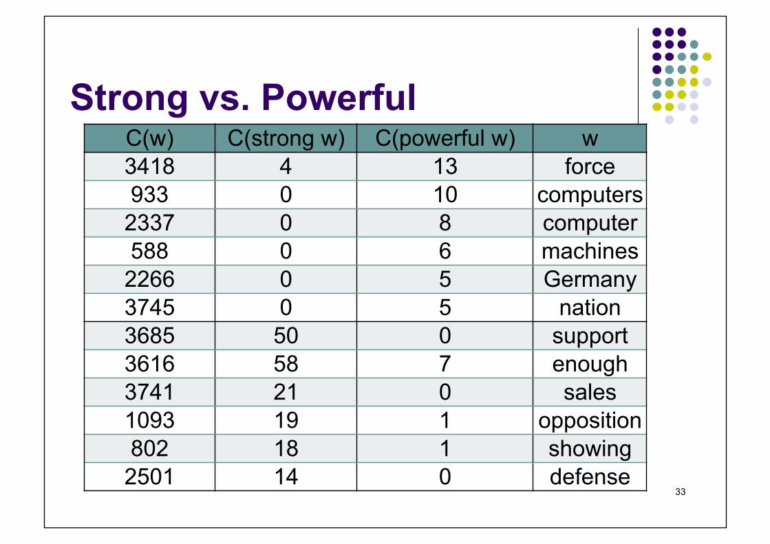
Strong vs. Powerful

 Are you drinking a “strong coffee” or a “powerful coffee”?  Are you working with a “strong PC” or a “powerful PC”?  Given the context, the translation could be “strong” or

“powerful” (but the distinction is not always (for a computer at least) very clear, e.g., “strong/powerful drug”)

 Based on newspaper articles, we can find

33

Strong vs. Powerful C(w) C(strong w) C(powerful w) w 3418 4 13 force 933 0 10 computers

2337 0 8 computer 588 0 6 machines

2266 0 5 Germany 3745 0 5 nation 3685 50 0 support 3616 58 7 enough 3741 21 0 sales 1093 19 1 opposition 802 18 1 showing

2501 14 0 defense

34

Conclusion

 Statistical tests could be useful to verify a theory  The interpretation and explanation of the underlying

phenomenon are not included in the test!  The Chi-square test could be used in various contexts  But

  random sampling   it needs at least 5 (expected) observations in each cell.