‘-

1

Chemical Engineering Plant Design

Lecture 01 Course Introduction & Flowsheets

Instructor: David Courtemanche

CE 408

‘-

2

Course Introduction

• Welcome to CE 408 Chemical Engineering Process Design

• This is a Capstone Course

• The course will deal with designing a chemical process and will draw from all of your chemical engineering

education

• We will be incorporating material from your entire curriculum• CE 212 Mass and energy balances

• CE 304 Thermodynamics

• CE 329 Reactors and kinetics

• CE 317 Fluid mechanics

• Particularly flow in pipes

• CE 318 Heat and Mass transfer

• CE 407 Separations

• We will be learning some new things, as well• Process simulation

• Evaporation

• Vacuum systems

• Project economics

• Heat exchanger network Pinch Analysis

‘-

3

Course Introduction

• A chemical Process Design Project is like an onion

• https://www.youtube.com/watch?v=aJQmVZSAqlc

• Yes, at times it will stink and it may make you cry…

• You start with identifying a business proposition

• Need to identify the market and customer requirements

• Identify required product specifications

• CE 404

• You identify ideas for what general process you will pursue

• Sketch out basic process steps

• Block flow diagrams

• Basic mass balances

• Start to identify specifications of required equipment

• Process Flow Diagrams

• Get general estimates of size and cost

• What are energy requirements?

• Begin economic evaluations

• Capital Costs / Raw material cost / energy costs / labor and overhead

• Revenue

• Is this a good investment?

‘-

4

Course Introduction

• A chemical Process Design Project is like an onion, continued

• This is an iterative process

• We will iterate in that as we get further into the details we’ll see original assumptions that

need to be changed

• We won’t see all of the gate keeping steps

• Design costs money – you don’t go ahead and just drive to a final design

• Evaluate the project economics with a plus/minus accuracy of perhaps 50%

• Use factors to account for all of the supporting equipment, installation costs, etc

• Do we pursue or not?

• More detailed design allows an estimate of perhaps plus/minus accuracy of 10%

• Safety and environmental considerations need to be considered by this point

• Higher detail allows better cost estimates of larger pieces of equipment

• Higher detail allows actual estimates of supporting equipment (you know what it is to a

better degree)

• Do we pursue or not?

• Final design allows an estimate of perhaps plus/minus accuracy of 5%

• Getting to the point where could actually build this plant with the level of design we have

• Decide to build it or not

‘-

5

Course Introduction

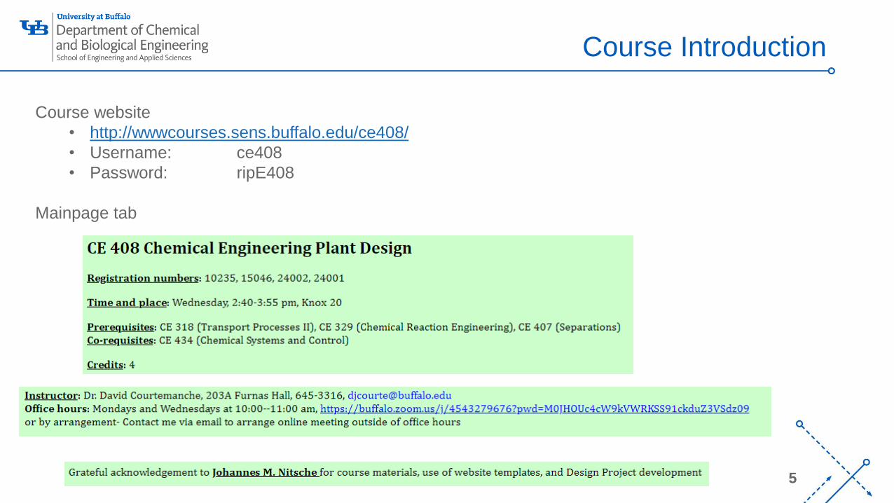
Course website

• http://wwwcourses.sens.buffalo.edu/ce408/

• Username: ce408

• Password: ripE408

Mainpage tab

‘-

6

Course Introduction

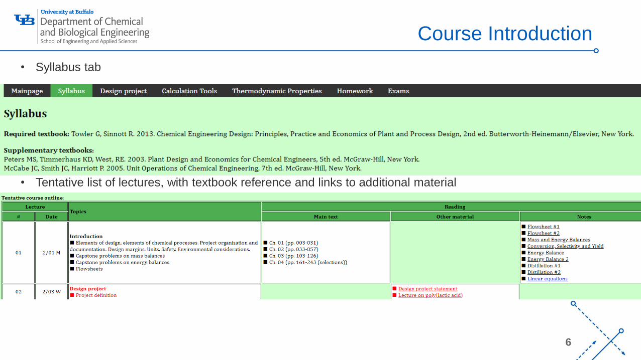
• Syllabus tab

• Tentative list of lectures, with textbook reference and links to additional material

‘-

7

Course Introduction

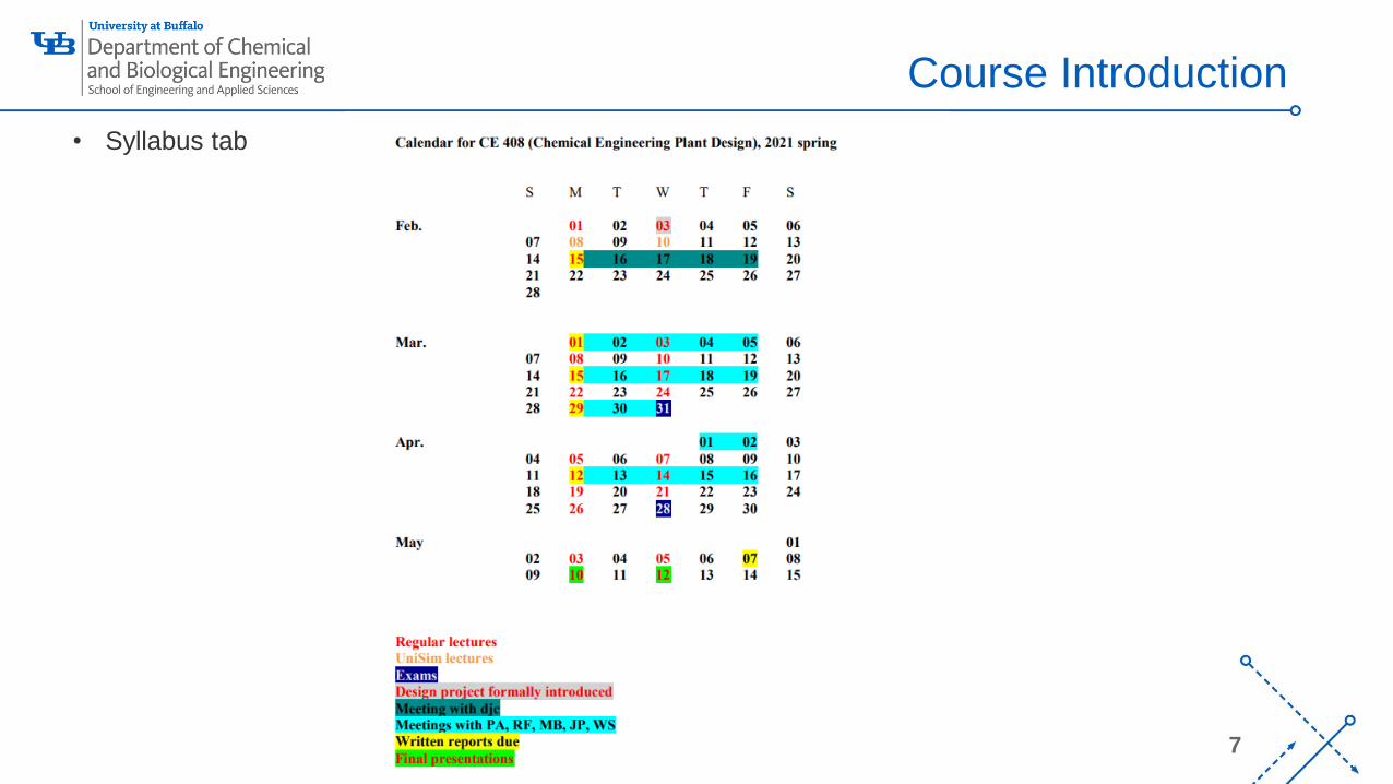
• Syllabus tab

‘-

8

Course Introduction

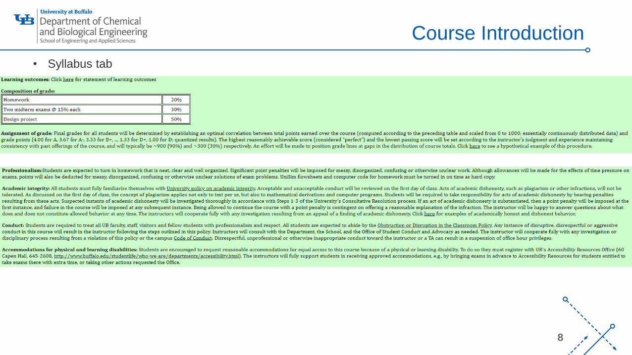
• Syllabus tab

‘-

9

Course Introduction

• Design Project Tab

• To be discussed in Lecture 2

‘-

10

Course Introduction

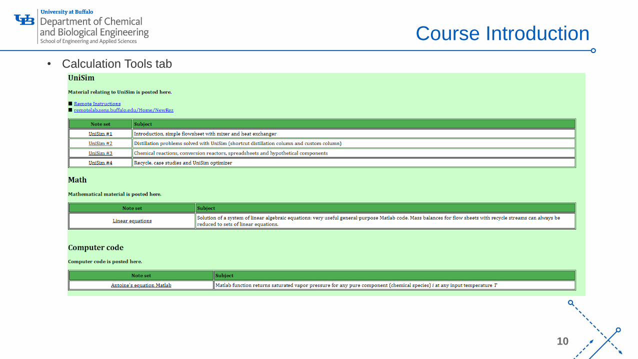
• Calculation Tools tab

‘-

11

Course Introduction

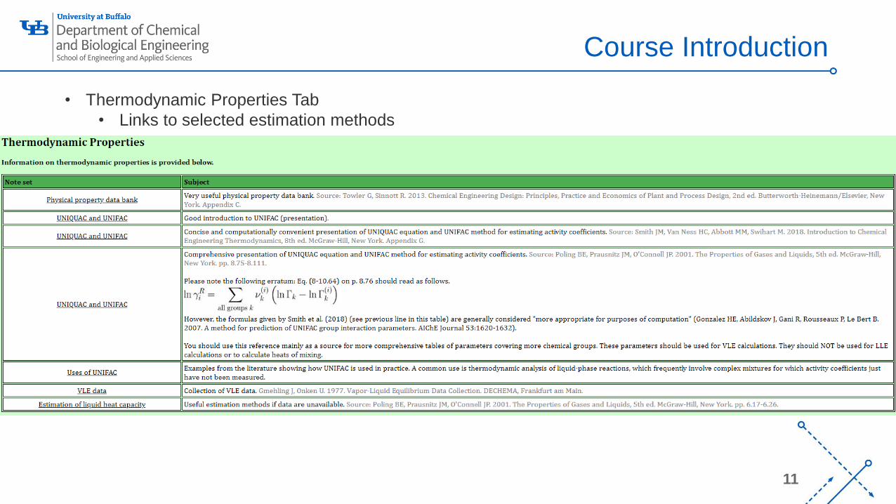
• Thermodynamic Properties Tab

• Links to selected estimation methods

‘-

12

Course Introduction

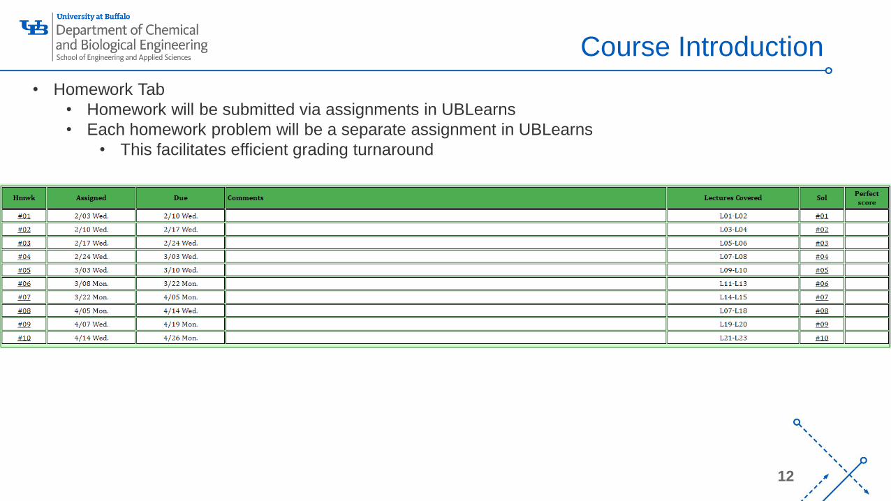
• Homework Tab

• Homework will be submitted via assignments in UBLearns

• Each homework problem will be a separate assignment in UBLearns

• This facilitates efficient grading turnaround

‘-

13

Course Introduction

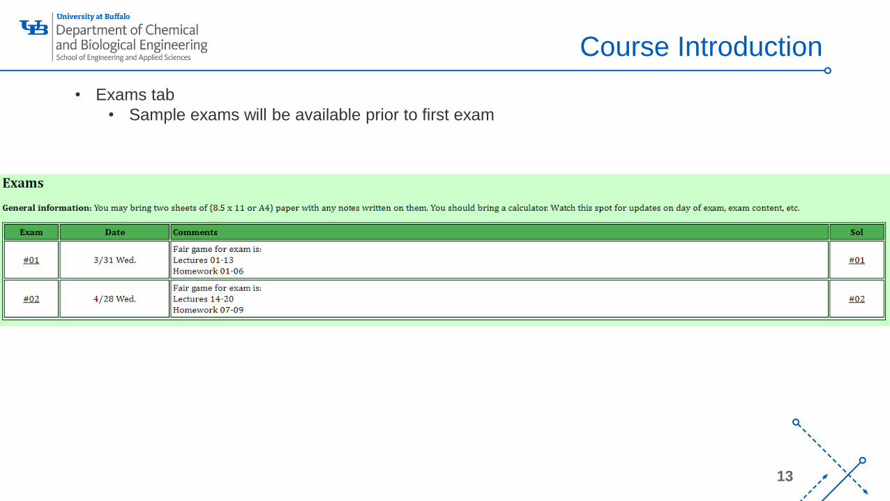
• Exams tab

• Sample exams will be available prior to first exam

‘-

14

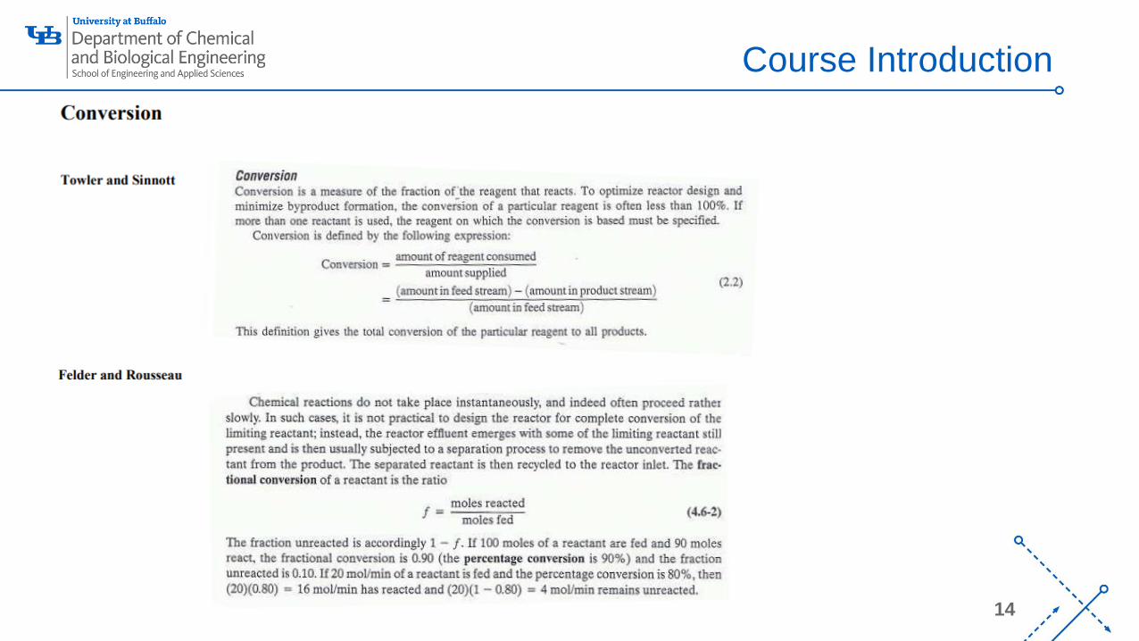
Course Introduction

‘-

15

Course Introduction

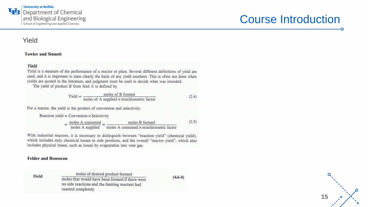
Yield

‘-

16

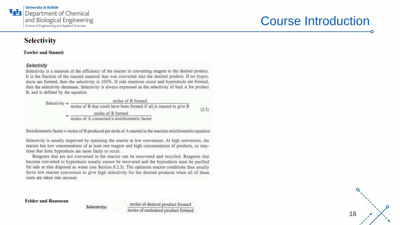
Course Introduction

‘-

17

Course Introduction

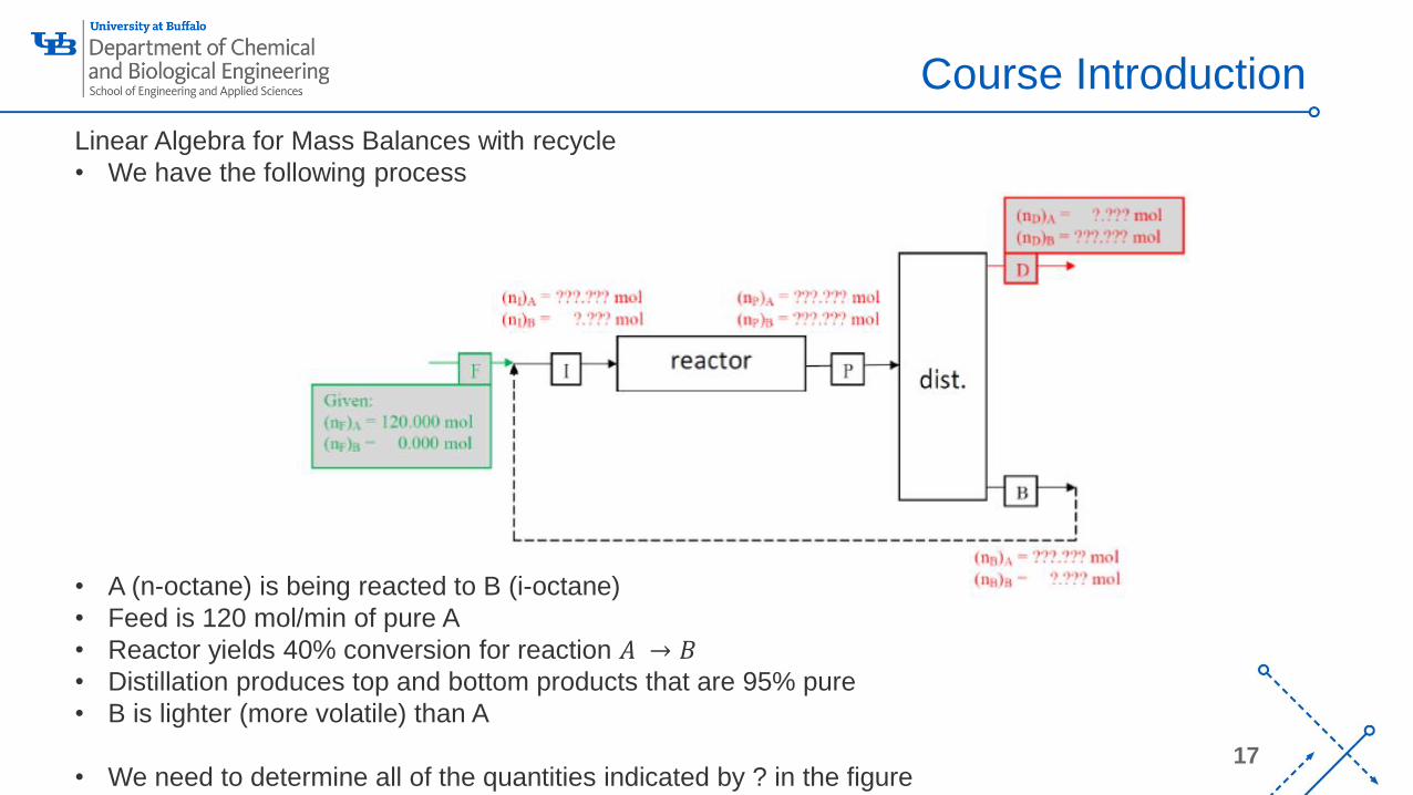
Linear Algebra for Mass Balances with recycle

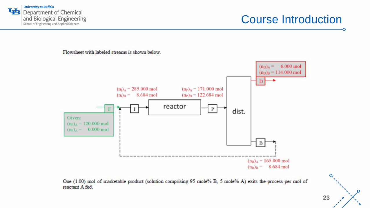
• We have the following process

• A (n-octane) is being reacted to B (i-octane)

• Feed is 120 mol/min of pure A

• Reactor yields 40% conversion for reaction 𝐴 → 𝐵• Distillation produces top and bottom products that are 95% pure

• B is lighter (more volatile) than A

• We need to determine all of the quantities indicated by ? in the figure

‘-

18

Course Introduction

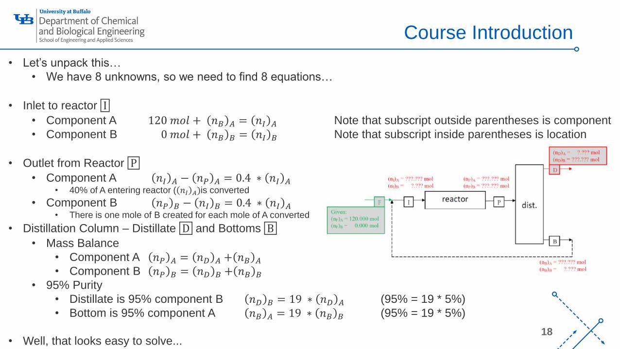
• Let’s unpack this…

• We have 8 unknowns, so we need to find 8 equations…

• Inlet to reactor I

• Component A 120 𝑚𝑜𝑙 + 𝑛𝐵 𝐴 = 𝑛𝐼 𝐴 Note that subscript outside parentheses is component

• Component B 0 𝑚𝑜𝑙 + 𝑛𝐵 𝐵 = 𝑛𝐼 𝐵 Note that subscript inside parentheses is location

• Outlet from Reactor P

• Component A 𝑛𝐼 𝐴 − 𝑛𝑃 𝐴 = 0.4 ∗ 𝑛𝐼 𝐴• 40% of A entering reactor ( 𝑛𝐼 𝐴)is converted

• Component B 𝑛𝑃 𝐵 − 𝑛𝐼 𝐵 = 0.4 ∗ 𝑛𝐼 𝐴• There is one mole of B created for each mole of A converted

• Distillation Column – Distillate D and Bottoms B

• Mass Balance

• Component A 𝑛𝑃 𝐴 = 𝑛𝐷 𝐴 + 𝑛𝐵 𝐴

• Component B 𝑛𝑃 𝐵 = 𝑛𝐷 𝐵 + 𝑛𝐵 𝐵

• 95% Purity

• Distillate is 95% component B 𝑛𝐷 𝐵 = 19 ∗ 𝑛𝐷 𝐴 (95% = 19 * 5%)

• Bottom is 95% component A 𝑛𝐵 𝐴 = 19 ∗ 𝑛𝐵 𝐵 (95% = 19 * 5%)

• Well, that looks easy to solve...

‘-

19

Course Introduction

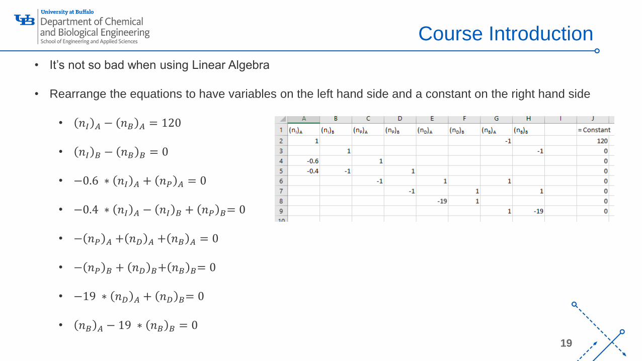
• It’s not so bad when using Linear Algebra

• Rearrange the equations to have variables on the left hand side and a constant on the right hand side

• 𝑛𝐼 𝐴 − 𝑛𝐵 𝐴 = 120

• 𝑛𝐼 𝐵 − 𝑛𝐵 𝐵 = 0

• −0.6 ∗ 𝑛𝐼 𝐴 + 𝑛𝑃 𝐴 = 0

• −0.4 ∗ 𝑛𝐼 𝐴 − 𝑛𝐼 𝐵 + 𝑛𝑃 𝐵= 0

• − 𝑛𝑃 𝐴 + 𝑛𝐷 𝐴 + 𝑛𝐵 𝐴 = 0

• − 𝑛𝑃 𝐵 + 𝑛𝐷 𝐵+ 𝑛𝐵 𝐵= 0

• −19 ∗ 𝑛𝐷 𝐴 + 𝑛𝐷 𝐵= 0

• 𝑛𝐵 𝐴 − 19 ∗ 𝑛𝐵 𝐵 = 0

‘-

20

Course Introduction

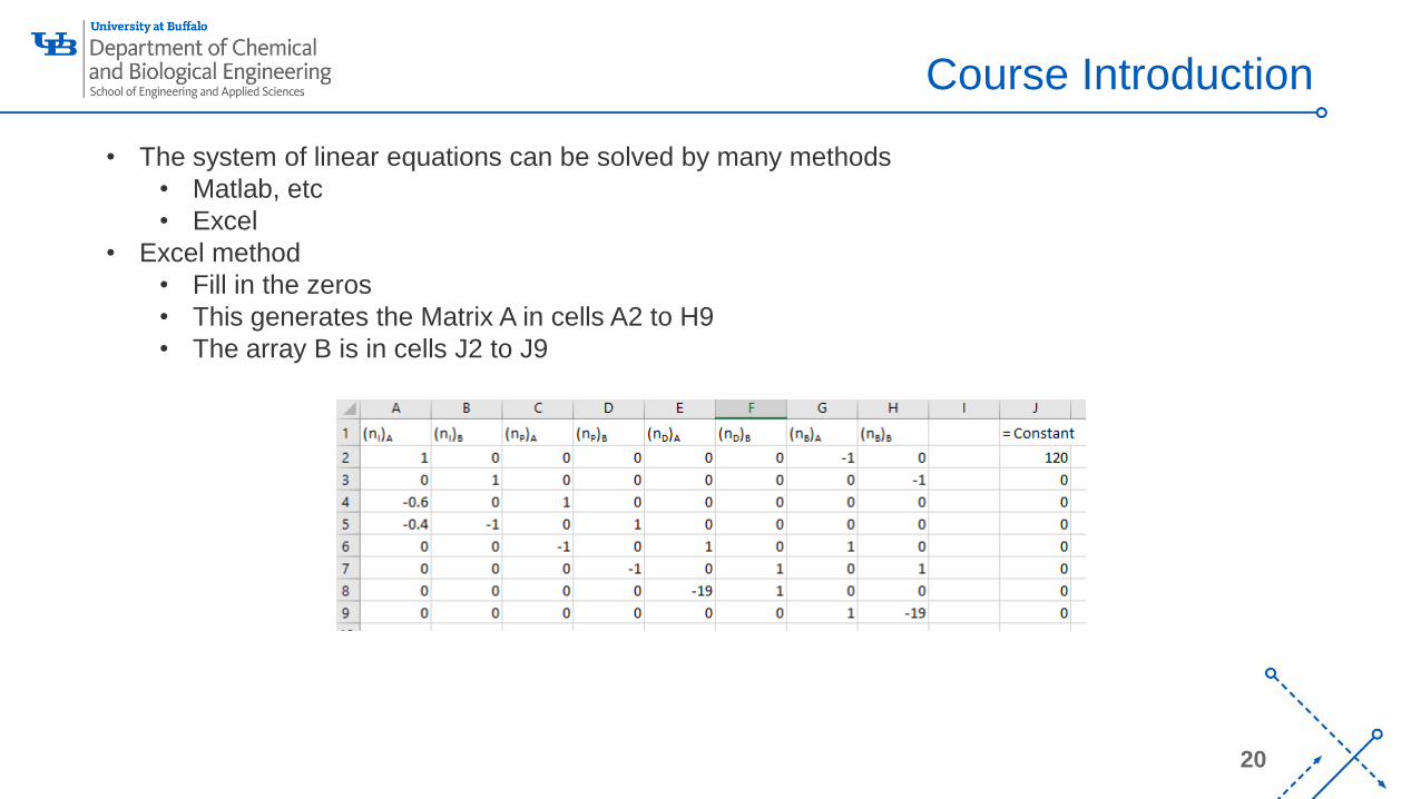
• The system of linear equations can be solved by many methods

• Matlab, etc

• Excel

• Excel method

• Fill in the zeros

• This generates the Matrix A in cells A2 to H9

• The array B is in cells J2 to J9

‘-

21

Course Introduction

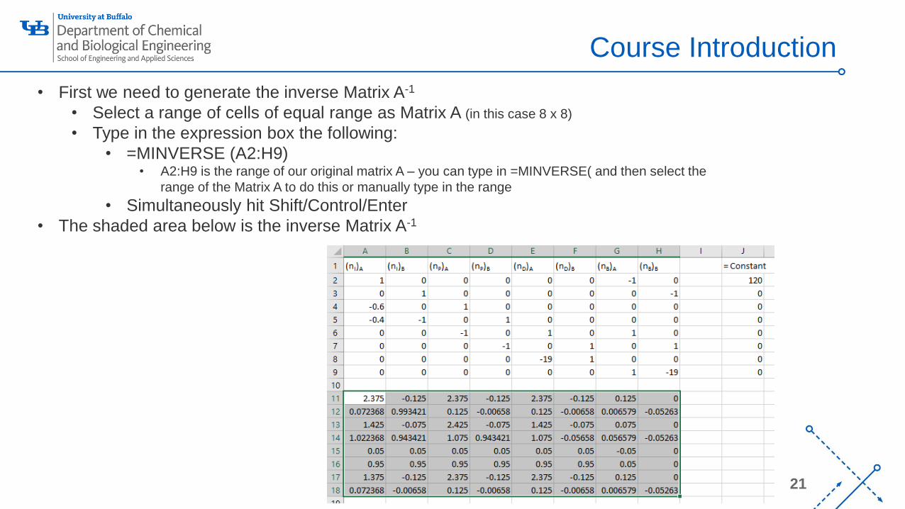
• First we need to generate the inverse Matrix A-1

• Select a range of cells of equal range as Matrix A (in this case 8 x 8)

• Type in the expression box the following:

• =MINVERSE (A2:H9) • A2:H9 is the range of our original matrix A – you can type in =MINVERSE( and then select the

range of the Matrix A to do this or manually type in the range

• Simultaneously hit Shift/Control/Enter

• The shaded area below is the inverse Matrix A-1

‘-

22

Course Introduction

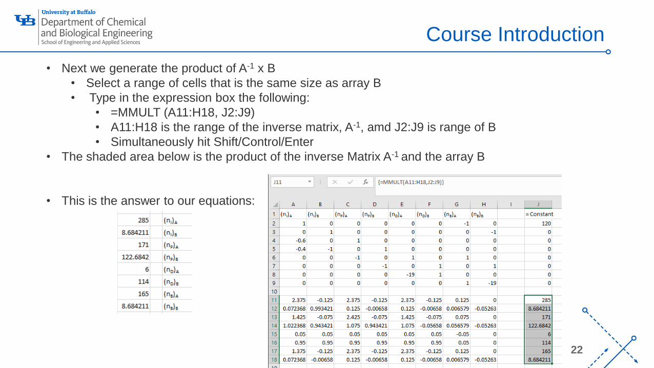
• Next we generate the product of A-1 x B

• Select a range of cells that is the same size as array B

• Type in the expression box the following:

• =MMULT (A11:H18, J2:J9)

• A11:H18 is the range of the inverse matrix, A-1, amd J2:J9 is range of B

• Simultaneously hit Shift/Control/Enter

• The shaded area below is the product of the inverse Matrix A-1 and the array B

• This is the answer to our equations:

‘-

23

Course Introduction