PNNL-14121

Characterization of Vadose Zone Sediment: RCRA Borehole 299-E33-338 Located Near the B-BX-BY Waste Management Area C.W. Lindenmeier M.J. Lindberg K.N. Geiszler R.J. Serne R.E. Clayton C.F. Brown B.N. Bjornstad V.L. LeGore M.M. Valenta G.W. Gee I.V. Kutnyakov T.S. Vickerman H.T. Schaef S.R. Baum L.J. Royack D.C. Lanigan June 2003 Prepared for CH2M Hill Hanford Group, Inc., and the U.S. Department of Energy under Contract DE-AC06-76RL01830

DISCLAIMER

This report was prepared as an account of work sponsored by an agency of the United States Government. Neither the United States Government nor any agency thereof, nor Battelle Memorial Institute, nor any of their employees, makes any warranty, express or implied, or assumes any legal liability or responsibility for the accuracy, completeness, or usefulness of any information, apparatus, product, or process disclosed, or represents that its use would not infringe privately owned rights. Reference herein to any specific commercial product, process, or service by trade name, trademark, manufacturer, or otherwise does not necessarily constitute or imply its endorsement, recommendation, or favoring by the United States Government or any agency thereof, or Battelle Memorial Institute. The views and opinions of authors expressed herein do not necessarily state or reflect those of the United States Government or any agency thereof.

PACIFIC NORTHWEST NATIONAL LABORATORY operated by BATTELLE

for the UNITED STATES DEPARTMENT OF ENERGY

under Contract DE-AC06-76RL01830

Printed in the United States of America

Available to DOE and DOE contractors from the Office of Scientific and Technical Information,

P.O. Box 62, Oak Ridge, TN 37831-0062; ph: (865) 576-8401 fax: (865) 576-5728

email: reports@adonis.osti.gov

Available to the public from the National Technical Information Service, U.S. Department of Commerce, 5285 Port Royal Rd., Springfield, VA 22161

ph: (800) 553-6847 fax: (703) 605-6900

email: orders@ntis.fedworld.gov online ordering: http://www.ntis.gov/ordering.htm

This document was printed on recycled paper. (8/00)

PNNL-14121

Characterization of Vadose Zone Sediment: RCRA Borehole 299-E33-338 Located Near the B-BX-BY Waste Management Area C.W. Lindenmeier M.J. Lindberg K.N. Geiszler R.J. Serne R.E. Clayton C.F. Brown B.N. Bjornstad V.L. LeGore M.M. Valenta G.W. Gee I.V. Kutnyakov T.S. Vickerman H.T. Schaef S.R. Baum L.J. Royack D.C. Lanigan June 2003 Prepared for CH2M HILL Hanford Group, Inc., and the U.S. Department of Energy under Contract DE-AC06-76RL01830 Pacific Northwest National Laboratory Richland, Washington 99352

iii

Executive Summary

The overall goals of the of the Tank Farm Vadose Zone Project, led by CH2M HILL Hanford Group, Inc., are: 1) to define risks from past and future single-shell tank farm activities, 2) to identify and evaluate the efficacy of interim measures, and 3) to aid via collection of geotechnical information and data, future decisions that must be made by the U.S. Department of Energy (DOE) regarding the near-term operations, future waste retrieval, and final closure activities for the single-shell tank waste management areas. For a more complete discussion of the goals of the Tank Farm Vadose Zone Project, see the overall work plan, Phase 1 RCRA Facility Investigation/Corrective Measures Study Work Plan for the Single-Shell Tank Waste Management Areas (DOE 1999). Specific details on the rationale for activities performed at the B-BX-BY tank farm waste management area are found in CH2M HILL (2000).

To meet these goals, CH2M HILL Hanford Group, Inc., asked scientists from Pacific Northwest National Laboratory to perform detailed analyses of vadose zone sediment, both uncontaminated and contaminated, from within B-BX-BY Waste Management Area.

Specifically, this report contains all the geologic, geochemical, and selected physical characterization data collected on vadose zone sediment recovered from the Resource Conservation and Recovery Act borehole 299-E33-338 that is near B-BX-BY Waste Management Area.

This report is one in a series of three reports to present recent data collected on vadose zone sediment that provides a baseline to compare with information from two contaminated boreholes within B-BX-BY Waste Management Area: 1) borehole 299-E33-45, and 2) borehole 299-E33-46 northeast of tank B-110, which has been decommissioned. This document describes all the characterization data collected and interpretations for borehole 299-E33-338 assembled by the Applied Geology and Geochemistry Group within the Environmental Technology Division of the Pacific Northwest National Laboratory and is incorporated in the B-BX-BY field investigation report.

The geology under the B-BX-BY Waste Management Area forms the framework through which the contaminants move, and as discussed in Serne et. al. 2002, provides the basis with which to interpret and extrapolate the physical and geochemical properties that control the migration and distribution of contaminants. Specifically, the identification of major lithological contacts and the interrelationships between the coarser- and finer-grained sediment facies are essential when combined with the geochemical profile for interpreting contaminant behavior in the subsurface. For this borehole, lithologic sections were constructed using detailed geologic descriptions, core photos, and geophysical logs. In some cases, the results of laboratory analyses (e.g. particle-size distribution, moisture, calcium carbonate content) helped refine the resulting stratigraphic and lithological interpretations.

Our conceptual model of the vadose zone associated with the 299 E33-338 borehole involves five distinct stratigraphic units beginning with the Hanford formation H1 unit from the surface to a depth of approximately 15.7 m (approximately 51.5-ft) described as a sandy gravel to gravelly sand sequence. This is followed by the Hanford formation H2 unit extending to a depth of approximately 57.9 m (109 ft) that is a sand sequence consisting of sand dominated facies, with multiple graded beds of horizontal to tabular cross-bedd sand to slightly gravelly sand. These graded beds are sometimes capped with thin

iv

layers of silty sand to silt. The last unit associated with the cataclysmic flood deposits is the Hanford H3 formation unit that extends to a depth of approximately 64.8 m (212.5 ft). It is a gravelly sand to slightly gravelly sand sequence. Just below the H3 unit is the Plio-Pleistocene silty unit (PPlz) extending to a depth of approximately 67.8 m (222.4 ft). This unit is a silt-dominated sequence consisting of interstratified well sorted silt and fine sand. The last unit characterized from this borehole was the Plio-Pleistocene gravelly unit (PPlg) extending to a depth of approximately 82.6 m (271 ft), however sampling ended at approximately 73.1 m (239.8 ft). This unit is differentiated from the PPlz due to its sandy gravel to gravelly sand sequence consisting predominantly of unconsolidated basalt-rich sand and gravel.

Sediment samples from the various stratigraphic unites were analyzed and characterized in the laboratory for the following parameters:

• Mass Water Content • Soil Suction • Particle-Size Distribution • Calcium Carbonate and Organic Carbon Contents • Bulk Chemical Composition • Mineralogy • Water Leach (1:1 sediment to water extraction) • Acid Leach (8M nitric acid extraction) Physical properties, such as particle size distribution and water content varied according to lithology

as expected. In general, elevated areas of water content (~ >5%) were typically associated with regions of fine grain sediments. Most notable are those regions involving lithological facies at which water contents equal or exceed 10%. Three major peaks are noted at 15.7, 52.9, and 67.1 m (51.6, 173.6, and 220.2 ft) bgs with water contents of 12.95, 14.27, and 26.02% respectively. Along with water content, soil suction measurements were made on most of the core liner and grab samples from the borehole using the filter paper method. Three major peaks were noted approximately 14, 64, and 73 m (45, 210, and 240 ft) bgs with suction measurements of approximately 1.3, 1.5, and 2.2 Mpa. The matric potential profile indicates that wetting from meteoric water has not reached the water table.

Inorganic carbon results reported in terms of calcium carbonate were found to be within the range of 0.5 to 2.0 wt %, and are consistent with results reported elsewhere (e.g. Serne et. al. 2002). The method used to measure the organic carbon relies on subtracting the inorganic carbon from the total carbon in the sample; for such low carbon values this method is not very accurate. The low values for organic carbon (0.01 to 0.14 %) are within the ranges generally reported for sediment at the Hanford site.

Bulk sediment samples were characterized for major and trace elements using a lithium metaborate/tetraborate fusion procedure, and then analyzed by inductively coupled plasma–optical emission spectroscopy (ICP-OES) and ICP-MS methods. Overall results showed very little difference in the primary elemental oxide concentrations for any of the sediment samples as a function of depth or lithology.

v

The water chemistry analysis for samples collected between 5 and 73 m (16 and 240 ft) bgs using the 1:1 soil to water extract method shows no strong trends as a function of depth and there is little, if any, indication of tank waste interaction with vadose zone soils at this location. Primary characteristics include the following:

• The 1:1 sediment-to-water extract pH varied from 6.97 to 7.74 and in general increased with depth with an average value of 7.4 (Figure 4.9 and Table 4.3).

• There were small increases in pH at the contact between the Hanford H2 and H3 units and the top and bottom of the Plio-Pleistocene mud unit.

• Porewater EC (dilution corrected) varied from 0.88 to 4.3 mS/cm with an average of 2.4 mS/cm.

• There were high EC values deep in the Hanford H2 unit at approximately 49 m (160 ft) bgs and in the deepest sample characterized (i.e., in the PPlg).

The shapes of the major cation profiles (sodium, potassium, calcium, magnesium, and strontium) in terms of calculated porewater concentration versus depth are very similar with slight peaks in the deep portion of the H2 unit at approximately 49 m (160 ft) bgs, at the top of the Plio-Pleistocene silty unit, and in the deepest sample characterized in the PPlg unit. All three of these samples had very low water contents and thus the dilution factor was high. The apparent high porewater concentrations likely represent some dissolution of salts from the sediment that are multiplied by a large dilution factor, and thus suggest more saline porewater than surrounding sediments with higher water content.

The shapes of the major anion profiles (fluoride, chloride, nitrate, bicarbonate, phosphate, and sulfate) in terms of calculated porewater concentration versus depth showed no consistent depths where all anions peaked unlike the major cation profiles. The wetter samples do consistently show low calculated porewater anion concentrations suggesting that the dilution factor is again controlling the apparent concentrations. That is, all the sediments likely dissolve some salts that are not truly in the porewater, so that the dilution correction makes it appear that the porewater anion concentrations are higher in the drier sediments.

This report is divided into sections that describe the geology, geochemical characterization methods employed, geochemical results, as well as summary and conclusions, references cited, and three appendices with additional details.

vii

Acknowledgements

This work was conducted as part of the Tank Farm Vadose Zone Project led by CH2M Hill Hanford Group, Inc., in support of the U.S. Department of Energy’s Office of River Protection. The authors wish to thank Anthony J. Knepp, Fredrick M. Mann, David A. Myers, Thomas E. Jones, and Harold A. Sydnor with CH2M Hill Hanford Group, Inc., Marc I. Wood and Raziuddin Khaleel with Fluor Hanford for their support of this work, and Kevin A. Lindey of Kennedy Jenkes Consultants, Inc. for his insights on the geological nature of the material penetrated by this borehole. We would also like to express our gratitude to Robert Yasek with U.S. Department of Energy’s Office of River Protection.

Finally, we would like to thank William J. Deutsch and Bruce J. Bjornstad for their technical review of this document, and Shanna K. Muns for her editorial and document production support.

ix

Contents

1.0 Introduction.................................................................................................................................. 1-1

2.0 Geology at Borehole 299-E33-338................................................................................................ 2-1 2.1 Hanford Formation ............................................................................................................... 2-7

2.1.1 Hanford Formation H1 Unit ....................................................................................... 2-7 2.1.2 Hanford Formation H2 Unit ....................................................................................... 2-7 2.1.3 Hanford Formation H3 Unit ..................................................................................... 2-10

2.2 Hanford Formation/Plio-Pleistocene (?) Unit ...................................................................... 2-11 2.2.1 Silt-Dominated Facies (PPlz) ................................................................................... 2-12 2.2.2 Sandy Gravel to Gravelly Sand Dominated Facies (PPlg) ......................................... 2-13

3.0 Characterization Analytical Methods ............................................................................................3-1 3.1 Geochemical and Analytical Laboratory Methods and Materials ........................................... 3-1

3.1.1 Borehole Core Sampling ............................................................................................ 3-1 3.1.2 Mass Water Content................................................................................................... 3-2 3.1.3 Particle Size Distribution ........................................................................................... 3-2 3.1.4 Particle Density.......................................................................................................... 3-3 3.1.5 1:1 Sediment-to-Water Extract ................................................................................... 3-3 3.1.6 8 M Nitric Acid Extract.............................................................................................. 3-3 3.1.7 pH and Conductivity .................................................................................................. 3-3 3.1.8 Anion Analysis .......................................................................................................... 3-3 3.1.9 Cations and Trace Metals ........................................................................................... 3-4 3.1.10 Alkalinity................................................................................................................... 3-4 3.1.11 Carbon Content.......................................................................................................... 3-4 3.1.12 Bulk Elemental Analysis ............................................................................................ 3-5 3.1.13 Mineralogy ................................................................................................................ 3-5 3.1.14 Water Potential (Suction) Measurements.................................................................... 3-7

4.0 Analytical Results for Sediment Samples...................................................................................... 4-1 4.1 Geophysical and Moisture Content Measurements ................................................................ 4-1 4.2 Particle Size Distribution and Particle Density ...................................................................... 4-6

4.2.1 Particle Size Distribution ........................................................................................... 4-6 4.2.2 Particle Density........................................................................................................ 4-14

4.3 Soil Water Chemistry Measurements .................................................................................. 4-14 4.4 Soil Fusion Analysis........................................................................................................... 4-32 4.5 Calcium Carbonate and Organic Carbon Content ................................................................ 4-43 4.6 Mineralogy......................................................................................................................... 4-44 4.7 Chemical Interactions ......................................................................................................... 4-49 4.8 Sediment Matric Potential at Borehole 299-E33-338........................................................... 4-49

x

5.0 Summary and Conclusions ........................................................................................................... 5-1

6.0 References.................................................................................................................................... 6-1

Appendix A – Summary of Field Geologists’ Sample Descriptions for Borehole 299-E33-338 ............ A.1 Appendix B – Summary of Geologists’ Core Sample Descriptions from Borehole 299-E33-338 .......... B-1 Appendix C – Summary of Geophysical Logs for Borehole 299-E33-338 ............................................ C-1

Figures

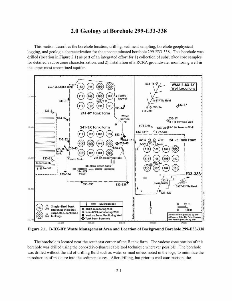
2.1 B-BX-BY Waste Management Area and Location of Background Borehole 299-E33-338........... 2-1 2.2 Borehole 299-E33-338 Lithology, Stratigraphy, Gamma, and Neutron Field Logs as a

Function of Depth ....................................................................................................................... 2-6 2.3 Core from the Hanford Formation H1 Unit in Borehole 299-E33-338.......................................... 2-7 2.4 Typical Hanford Formation H2 Unit in Borehole 299-E33-338.................................................... 2-8 2.5 Lower Fine-Grained Layer in the Hanford Formation H2 Unit..................................................... 2-9 2.6 Hanford Formation H3 Unit in Borehole 299-E33-338 .............................................................. 2-10 2.7 Weak Paleosol Within the Hanford Formation H3 Unit in Borehole 299-E33-338 ..................... 2-11 2.8 Upper Bed in Plio-Pleistocene Silt Facies in Borehole 299-E33-338.......................................... 2-12 2.9 Lower Bed in Plio-Pleistocene Silt Facies in Borehole 299-E33-338 ......................................... 2-13 2.10 Sandy Gravel to Gravelly Sand-Dominated Facies of the Plio-Pleistocene unit in

Borehole 299-E33-338 .............................................................................................................. 2-14 3.1 Sediment Textural Classification................................................................................................. 3-2 4.1 Borehole 299-E33-338 Lithology, Stratigraphy, Field Logs, and Moisture Distribution as a

Function of Depth ....................................................................................................................... 4-5 4.2 Particle Size Distribution 15.5-51.05 ft bgs.................................................................................. 4-7 4.3 Particle Size Distribution 77.3-115.4 ft bgs.................................................................................. 4-8 4.4 Particle Size Distribution 133-173.05 ft bgs................................................................................. 4-9 4.5 Particle Size Distribution 198.15-200.1 ft bgs............................................................................ 4-10 4.6 Particle Size Distribution 213.8-219.7 ft bgs.............................................................................. 4-11 4.7 Particle Size Distribution 219-239.8 ft bgs. ............................................................................... 4-12 4.8 Overall Gravel, Sand, and Silt/Clay Composition for 299-E33-338............................................ 4-13 4.9 Borehole 299-E33-338 Lithology, Stratigraphy, and Moisture, Extract pH and Calculated

Porewater Electrical Conductivity Distribution as a Function of Depth. ..................................... 4-16 4.10 Calculated Cation Porewater Content for Borehole 299-E33-338 as a Function of Depth........... 4-18 4.11 Calculated Aluminum, Barium, Iron, Silicon, and Uranium Porewater Content for Borehole

299-E33-338 as a Function of Depth ......................................................................................... 4-19 4.12 Water and Acid Extractable Concentrations of Selected Constituents for Borehole

299-E33-338 as a Function of Depth ......................................................................................... 4-30 4.13 Water and Acid Extractable Concentrations of Trace Constituents for Borehole

299-E33-338 as a Function of Depth ......................................................................................... 4-31 4.14 XRD Tracing of Sediment Collected from 198.1 ft, Along With the Standard Reference

Patterns for Quartz and Plagioclase. .......................................................................................... 4-45

xi

4.15 XRD Tracings of Preferentially Oriented Clay Slide Taken from Borehole 299-E33-338 at a Depth of 198.1 ft ................................................................................................................ 4-48

4.16 Matric Potential of the Sediment Profile at Borehole 299-E33-338. ........................................... 4-50

Tables

2.1 Sub-sampled Split-Spoon Cores from Borehole 299-E33-338 Analyzed for Mineralogy and Geochemistry.............................................................................................................................. 2-3

2.2 Stratigraphic Terminology Used for the Vadose Zone in the Vicinity of the B, BX, and BY Tank Farms. ......................................................................................................................... 2-5

4.1 Moisture Content of Sediments in Borehole 299-E33-338 ........................................................... 4-1 4.2 Particle Densities for Selected Samples from Borehole 299-E33-338......................................... 4-14 4.3 Water Extract pH and Calculated Porewater Electrical Conductivity Values for

Borehole 299-E33-338. ............................................................................................................. 4-15 4.4 Calculated Cation Porewater Content for Borehole 299-E33-338............................................... 4-20 4.5 Calculated Porewater Trace Metal Composition for Water Extracts of Sediment. ...................... 4-22 4.6 Calculated Anion Porewater Content for Borehole 299-E33-338. .............................................. 4-23 4.7 Water Extract of Major Cations in Terms of Dry Sediment (µg/g). ............................................ 4-26 4.8 Acid Extract of Major Cations in Terms of Dry Sediment (µg/g). .............................................. 4-28 4.9 Element Constituents from Soil Fusion Method......................................................................... 4-33 4.10 Calcium Carbonate and Organic Carbon Content....................................................................... 4-43 4.11 Semi-quantitative XRD Results of Minerals from Borehole 299-E33-338.................................. 4-46 4.12 Semi-quantitative XRD Results of Clay Minerals Separated from the Sediment Collected

from Borehole 299-E33-338...................................................................................................... 4-49

xiii

Acronyms and Abbreviations

ASA American Society of Agronomy ASTM American Society of Testing and Materials bgs below ground surface DOE U.S. Department of Energy EC electrical conductivity EPA U.S. Environmental Protection Agency ESL PNNL Environmental Sciences Laboratory FIR field investigation report GEA gamma energy analysis HCl hydrochloric acid Hf/PPu Hanford formation/Plio-Pleistocene unit (?) Hf/PP/R Hanford formation/Plio-Pleistocene unit/Ringold formation(?) IC ion chromatography ICP inductively coupled plasma ICP-MS inductively coupled plasma -mass spectrometer ICP-OES inductively coupled plasma –optical emission spectroscopy PNNL Pacific Northwest National Laboratory PPlg Plio-Pleistocene unit gravelly sand or sandy gravel facies PPlz Plio-Pleistocene unit mud facies RCRA Resource Conservation and Recovery Act TEM transmission electron microscopy WMA Waste Management Area XRD x-ray diffraction

1-1

1.0 Introduction

In fiscal year 1999, several offices within the U.S. Department of Energy (DOE) initiated and funded coordinated activities at the Hanford Reservation to study the vadose zone to better understand the fate of contaminants that have leaked from underground storage tanks. As part of this effort, the Pacific Northwest National Laboratory (PNNL) under the direction of CH2M Hill Hanford Group, Inc. (CH2M HILL), received intact sediment cores from the subsurface immediately adjacent to the B-BX-BY Waste Management Area (WMA). These cores were collected during the installation of a new Resource Conservation and Recovery Act (RCRA) groundwater monitoring well 299-E33-338. Location maps and more details on the sampling location are presented in Section 2.0.

The clean borehole samples from this effort were collected for analysis of their physical, mineralogical, and chemical properties to serve as a Hanford Site standard for the B-BX-BY WMA. The characterized core samples are available to researchers for experiments relative to environmental problems at the Hanford Site. To obtain sediment, contact Clark Lindenmeier at PNNL by the following venues: telephone (509) 376-8419, fax (509) 376-5368, or email clark.Lindenmeier@pnl.gov.

This report summarizes data measured for samples collected from borehole 299-E33-338 (C3391). Borehole 299-E33-338 was drilled for two purposes: 1) for installation of a RCRA groundwater monitoring well (Horton 2002) and 2) to characterize the in situ soils and background porewater chemistry near the B-BX-BY WMA that have been largely uncontaminated by tank farm and crib and trench discharge operations. This borehole was drilled just outside the southeast fence line of the B tank farm (Figure 2.1). The borehole was drilled between July 23 and August 8, 2001 to a total depth of 80.05 m (275.75 ft) below ground surface (bgs) using the cable-tool method (Horton 2002). The water table was contacted at 77.5 m (254.2 ft) bgs and the top of basalt at 82.6 m (271 ft) bgs. Samples to the top of basalt were collected using drive barrel/splitspoon techniques, before switching to a hard tool to drill 1.5 m (5 ft) into the basalt.

Nearly continuous core was obtained down to a depth of approximately 78.6 m (258 ft) bgs. Two hundred and two 1-ft long by 4-in. diameter cores were retrieved, which accounts for approximately 75% of the total length of the borehole. Each 2-ft splitspoon contained two 1-ft Lexan-lined core segments. The lithology of this borehole was summarized onto a field geologist’s log by a Fluor Hanford, Inc. geologist (L. D. Walker). Subsequently, visual inspection of the cores was performed in the laboratory by K. A. Lindsey (Kennedy / Jenks), K. D. Reynolds (Duratek Federal Services), and B. N. Bjornstad (PNNL), who also collected 24 samples for paleomagnetic analysis.

Sub-samples were taken from all 202 cores for moisture content (Table 4-1). In addition, 21 core sub-samples were collected from depths of geological interest for mineralogical and geochemical analysis. Data from these samples allow for comparison of uncontaminated versus contaminated soils to better understand the contributions of tank wastes and other wastewaters on the vadose zone in and around B-BX-BY WMA.

1-2

The primary characterization activities included:

• Mass Water Content • Soil Suction • Particle-Size Distribution • Calcium Carbonate and Organic Carbon Contents • Bulk Chemical Composition • Mineralogy • Water Leach (1:1 sediment to water extraction) • Acid Leach (8M nitric acid extraction)

Support for this work was provided by CH2M Hill Hanford Group, Inc., specifically the Tank Farm Vadose Zone Project. The overall goal of the Tank Farm Vadose Zone Project is to define risks from past and future single-shell tank farm activities, to identify and evaluate the efficacy of interim measures, and to aid future decisions that must be made by DOE regarding the near-term operations, future waste retrieval, and final closure activities for the single-shell tank WMAs. For a more complete discussion of the goals of the Tank Farm Vadose Zone Project, see the overall work plan, Phase 1 Resource Conservation and Recovery Act (RCRA) Facility Investigation/Corrective Measures Study Work Plan for the Single-Shell Tank Waste Management Areas (DOE/RL 1999).

This report is divided into sections that describe the geology, geochemical characterization methods

employed, geochemical results, as well as summary and conclusions, references cited, and three appendices with additional details.

2-1

2.0 Geology at Borehole 299-E33-338

This section describes the borehole location, drilling, sediment sampling, borehole geophysical logging, and geologic characterization for the uncontaminated borehole 299-E33-338. This borehole was drilled (location in Figure 2.1) as part of an integrated effort for 1) collection of subsurface core samples for detailed vadose zone characterization, and 2) installation of a RCRA groundwater monitoring well in the upper most unconfined aquifer.

Figure 2.1. B-BX-BY Waste Management Area and Location of Background Borehole 299-E33-338

The borehole is located near the southeast corner of the B tank farm. The vadose zone portion of this

borehole was drilled using the core-(drive-)barrel cable tool technique wherever possible. The borehole was drilled without the aid of drilling fluid such as water or mud unless noted in the logs, to minimize the introduction of moisture into the sediment cores. After drilling, but prior to well construction, the

2-2

borehole was geophysically logged with spectral gamma (i.e., total gamma and potassium, uranium, thorium [KUT], and neutron-neuton [moisture]) probes. Borehole sampling consisted of near continuous split-spoon coring and/or sediment grab sampling throughout the borehole. Sediment cores were collected by driving a 10-cm (4-in.)-diameter 76-cm (2.5 ft)-long split-spoon sampling device ahead of the drilled borehole. The borehole was then cleaned to the bottom of the cored interval prior to the next sampling interval. Field borehole logs indicate that hard tool drilling began at approximately 82.6 m (271 ft) at the top of the basalt and continued to a final depth of approximately 84 m (275.5 ft). Each split-spoon core run contained in two capped 30 cm (1 ft) long, transparent, Lexan liners (core sleeves). Core recovery was generally 100%, however, in gravelly intervals such as in the first 4.6 m (15 ft), recovery was as low as 40%. All cores were sealed and labeled in the field and transported in ice chests to the PNNL environmental sciences laboratory (ESL) in the 3720 Building (300 Area) for refrigerated storage and further sampling and analysis.

In addition to Lexan-lined core samples, sediment grab samples were collected in the field from cuttings recovered during drilling and/or from the 0.5 ft-long split-spoon drive shoe. Several types of samples were labeled and contained from each sample interval. Samples for geologic descriptions were collected in 2.5 cm (1 in.) plastic sample chip trays from surface to total depth. With the exception of the drive shoe grab samples, most of the grab samples are composite samples composed of sediment that was churned up and mixed during the drilling and sampling process.

Lexan-lined cores provide the most representative intact samples of the subsurface and the core depth intervals are believed to be accurate to within 15 cm (0.5 ft) of actual depth. Geophysical logs were used to verify contacts. Fine sediment structure is usually well preserved in the split-spoon cores although layering may be deformed along sides of core due to drag. In the laboratory, the Lexan liners were cut lengthwise with a saw and the core was split into two slabs or halves. Sub-samples for physical and geochemical characterization were collected from the middle (inside) of the core slabs.

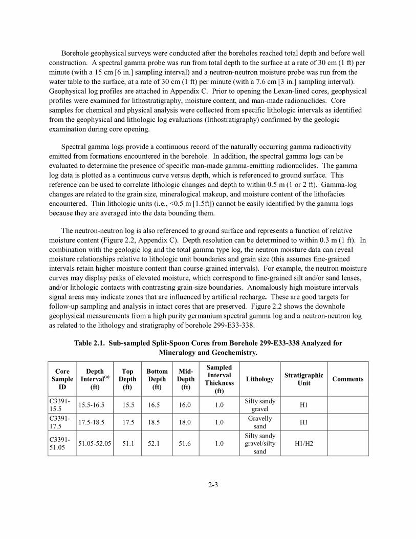
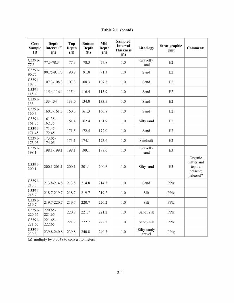
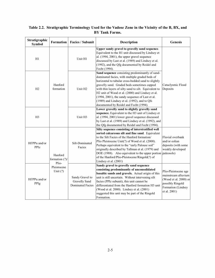
A field geologist prepared a geologic description (lithologic log) during drilling and coring of the borehole (Appendix A). The lithologic descriptions were based on visual inspection of material from the split-spoon core shoe, drill cutting, and grab samples. These logs provide a general indication of the lithology encountered. In addition to these field descriptions, a more rigorous and detailed analysis of the vadose zone stratigraphy was performed by geologists in the laboratory, based on cores observed within opened Lexan liners. Appendix B provides the borehole geologic log for 299-E33-338, which was created based on the examination of every third or fourth intact split-spoon core (opened in the laboratory). Table 2.1 provides a summary of the geologist’s laboratory assessment of the lithology and stratigraphy for those samples that were selected for detailed geochemical and physical properties characterization. Table 2.2 provides the generalized stratigraphic nomenclature relative to the lithological descriptions used throughout this report.

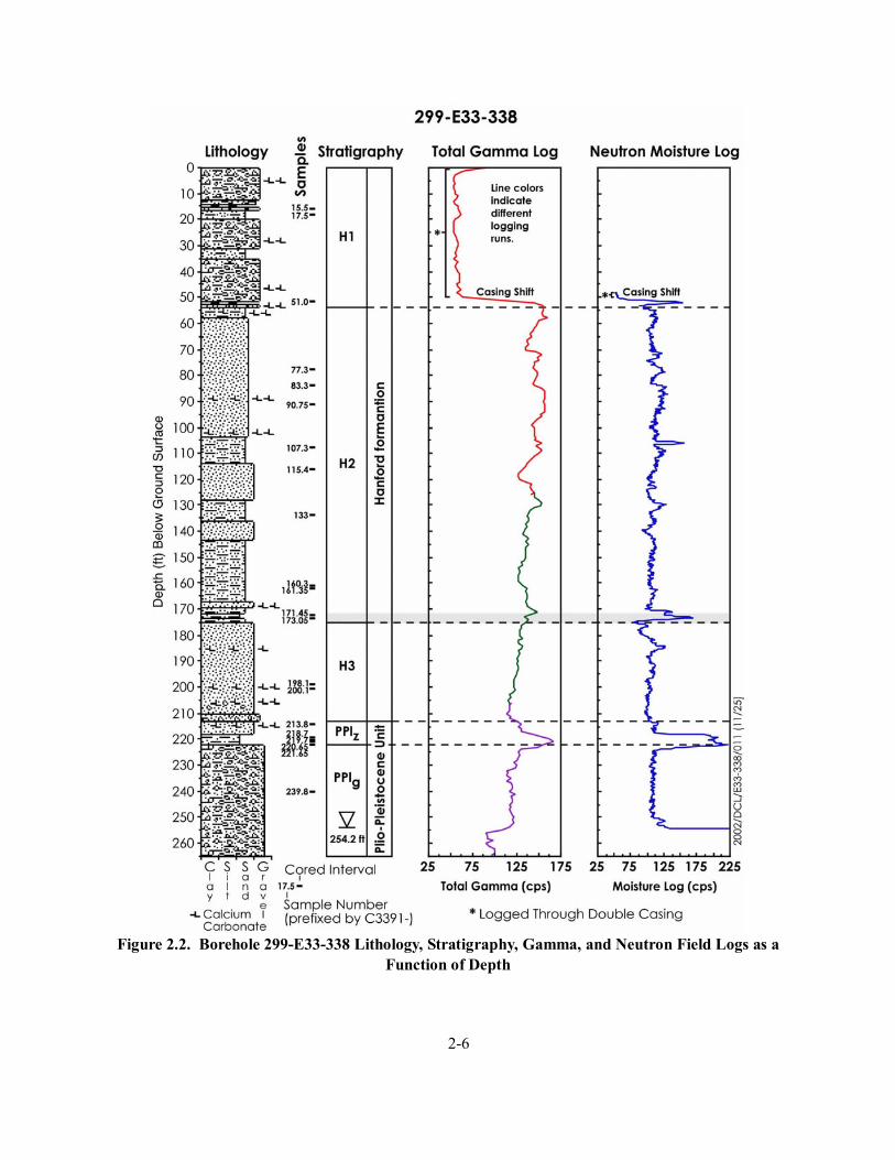
Two principal stratigraphic units are represented in borehole 299-E33-338, the Hanford formation and the Plio-Pleistocene unit (Table 2.2). The top of basalt was encountered at 82.6 m (271 ft) bgs. The vadose zone is approximately 77.5 m (254 ft) thick and the underlying unconfined aquifer is approximately 5.2 m (17 ft) thick. Zones with elevated moisture occur at several locations within the vadose zone; these occur along sharp lithologic boundaries, often in combination with finer-grained intervals (Figure 2.2).

2-3

Borehole geophysical surveys were conducted after the boreholes reached total depth and before well construction. A spectral gamma probe was run from total depth to the surface at a rate of 30 cm (1 ft) per minute (with a 15 cm [6 in.] sampling interval) and a neutron-neutron moisture probe was run from the water table to the surface, at a rate of 30 cm (1 ft) per minute (with a 7.6 cm [3 in.] sampling interval). Geophysical log profiles are attached in Appendix C. Prior to opening the Lexan-lined cores, geophysical profiles were examined for lithostratigraphy, moisture content, and man-made radionuclides. Core samples for chemical and physical analysis were collected from specific lithologic intervals as identified from the geophysical and lithologic log evaluations (lithostratigraphy) confirmed by the geologic examination during core opening.

Spectral gamma logs provide a continuous record of the naturally occurring gamma radioactivity emitted from formations encountered in the borehole. In addition, the spectral gamma logs can be evaluated to determine the presence of specific man-made gamma-emitting radionuclides. The gamma log data is plotted as a continuous curve versus depth, which is referenced to ground surface. This reference can be used to correlate lithologic changes and depth to within 0.5 m (1 or 2 ft). Gamma-log changes are related to the grain size, mineralogical makeup, and moisture content of the lithofacies encountered. Thin lithologic units (i.e., <0.5 m [1.5ft]) cannot be easily identified by the gamma logs because they are averaged into the data bounding them.

The neutron-neutron log is also referenced to ground surface and represents a function of relative moisture content (Figure 2.2, Appendix C). Depth resolution can be determined to within 0.3 m (1 ft). In combination with the geologic log and the total gamma type log, the neutron moisture data can reveal moisture relationships relative to lithologic unit boundaries and grain size (this assumes fine-grained intervals retain higher moisture content than course-grained intervals). For example, the neutron moisture curves may display peaks of elevated moisture, which correspond to fine-grained silt and/or sand lenses, and/or lithologic contacts with contrasting grain-size boundaries. Anomalously high moisture intervals signal areas may indicate zones that are influenced by artificial recharge. These are good targets for follow-up sampling and analysis in intact cores that are preserved. Figure 2.2 shows the downhole geophysical measurements from a high purity germanium spectral gamma log and a neutron-neutron log as related to the lithology and stratigraphy of borehole 299-E33-338.

Table 2.1. Sub-sampled Split-Spoon Cores from Borehole 299-E33-338 Analyzed for Mineralogy and Geochemistry.

Core Sample

ID

Depth Interval(a)

(ft)

Top Depth

(ft)

Bottom Depth

(ft)

Mid-Depth

(ft)

Sampled Interval

Thickness (ft)

Lithology Stratigraphic Unit Comments

C3391-15.5 15.5-16.5 15.5 16.5 16.0 1.0 Silty sandy

gravel H1

C3391-17.5 17.5-18.5 17.5 18.5 18.0 1.0 Gravelly

sand H1

C3391-51.05 51.05-52.05 51.1 52.1 51.6 1.0

Silty sandy gravel/silty

sand H1/H2

2-4

Table 2.1 (contd)

Core Sample

ID

Depth Interval(a)

(ft)

Top Depth

(ft)

Bottom Depth

(ft)

Mid-Depth

(ft)

Sampled Interval

Thickness (ft)

Lithology Stratigraphic Unit Comments

C3391-77.3 77.3-78.3 77.3 78.3 77.8 1.0 Gravelly

sand H2

C3391-90.75 90.75-91.75 90.8 91.8 91.3 1.0 Sand H2

C3391-107.3 107.3-108.3 107.3 108.3 107.8 1.0 Sand H2

C3391-115.4 115.4-116.4 115.4 116.4 115.9 1.0 Sand H2

C3391-133 133-134 133.0 134.0 133.5 1.0 Sand H2

C3391-160.3 160.3-161.3 160.3 161.3 160.8 1.0 Sand H2

C3391-161.35

161.35-162.35 161.4 162.4 161.9 1.0 Silty sand H2

C3391-171.45

171.45-172.45 171.5 172.5 172.0 1.0 Sand H2

C3391-173.05

173.05-174.05 173.1 174.1 173.6 1.0 Sand/silt H2

C3391-198.1 198.1-199.1 198.1 199.1 198.6 1.0 Gravelly

sand H3

C3391-200.1 200.1-201.1 200.1 201.1 200.6 1.0 Silty sand H3

Organic matter and

tephra present;

paleosol? C3391-213.8 213.8-214.8 213.8 214.8 214.3 1.0 Sand PPlz

C3391-218.7 218.7-219.7 218.7 219.7 219.2 1.0 Silt PPlz

C3391-219.7 219.7-220.7 219.7 220.7 220.2 1.0 Silt PPlz

C3391-220.65

220.65-221.65 220.7 221.7 221.2 1.0 Sandy silt PPlz

C3391-221.65

221.65-222.65 221.7 222.7 222.2 1.0 Sandy silt PPlz

C3391-239.8 239.8-240.8 239.8 240.8 240.3 1.0 Silty sandy

gravel PPlg

(a) multiply by 0.3048 to convert to meters

2-5

Table 2.2. Stratigraphic Terminology Used for the Vadose Zone in the Vicinity of the B, BX, and BY Tank Farms.

Stratigraphic Symbol Formation Facies / Subunit Description Genesis

H1 Unit H1

Upper sandy gravel to gravelly sand sequence. Equivalent to the H1 unit discussed by Lindsey et al. (1994, 2001), the upper gravel sequence discussed by Last et al. (1989) and Lindsey et al. (1992), and the Qfg documented by Reidel and Fecht (1994).

H2 Unit H2

Sand sequence consisting predominantly of sand-dominated facies, with multiple graded beds of horizontal to tabular cross-bedded sand to slightly gravelly sand. Graded beds sometimes capped with thin layers of silty sand to silt. Equivalent to H2 unit of Wood et al. (2000) and Lindsey et al. (1994, 2001), the sandy sequence of Last et al. (1989) and Lindsey et al. (1992), and to Qfs documented by Reidel and Fecht (1994).

H3

Hanford formation

Unit H3

Lower gravelly sand to slightly gravelly sand sequence. Equivalent to the H3 unit of Lindsey et al. (1994, 2001) lower gravel sequence discussed by Last et al. (1989) and Lindsey et al. (1992), and the Qfg documented by Reidel and Fecht (1994).

Cataclysmic Flood Deposits

Hf/PPu and/or PPlz

Silt-Dominated Facies

Silty sequence consisting of interstratified well sorted calcareous silt and fine sand. Equivalent to the Silt Facies of the Hanford formation/ Plio Pleistocene Unit(?) of Wood et al. (2000). Perhaps equivalent to the “early Palouse soil” originally described by Tallman et al. (1979) and DOE (1988). Also equivalent to the upper portion of the Hanford/Plio-Pleistocene/Ringold(?) of Lindsey et al. (2001)

Fluvial overbank and/or eolian deposits (with some weakly developed paleosols)

Hf/PPu and/or PPlg

Hanford formation (?)/

Plio-Pleistocene

Unit (?)

Sandy Gravel to Gravelly Sand

Dominated Facies

Sandy gravel to gravelly sand sequence consisting predominantly of unconsolidated basaltic sands and gravels. Actual origin of this unit is still uncertain. Without intervening silt facies (PPlz subunit), this unit cannot be differentiated from the Hanford formation H3 unit (Wood et al. 2000). Lindsey et al. (2001) suggested this unit may be part of the Ringold Formation.

Plio-Pleistocene age mainstream alluvium (Wood et al. 2000) or possibly Ringold Formation (Lindsey et al. 2001)

2-6

Figure 2.2. Borehole 299-E33-338 Lithology, Stratigraphy, Gamma, and Neutron Field Logs as a

Function of Depth

2-7

2.1 Hanford Formation

Wood et al. (2000) and Lindsey et al. (2001) describe cataclysmic flood deposits of the Hanford formation in the vicinity of the 241-B, BX, and BY tank farms as consisting of three informal units (i.e., H1, H2, and H3). Following is a description of these units within borehole 299-E33-338.

2.1.1 Hanford Formation H1 Unit

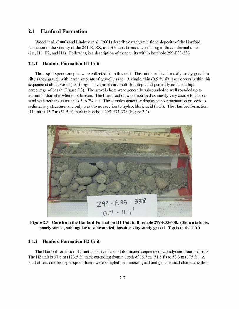
Three split-spoon samples were collected from this unit. This unit consists of mostly sandy gravel to silty sandy gravel, with lesser amounts of gravelly sand. A single, thin (0.5 ft) silt layer occurs within this sequence at about 4.6 m (15 ft) bgs. The gravels are multi-lithologic but generally contain a high percentage of basalt (Figure 2.3). The gravel clasts were generally subrounded to well rounded up to 50 mm in diameter where not broken. The finer fraction was described as mostly very coarse to coarse sand with perhaps as much as 5 to 7% silt. The samples generally displayed no cementation or obvious sedimentary structure, and only weak to no reaction to hydrochloric acid (HCl). The Hanford formation H1 unit is 15.7 m (51.5 ft) thick in borehole 299-E33-338 (Figure 2.2).

Figure 2.3. Core from the Hanford Formation H1 Unit in Borehole 299-E33-338. (Shown is loose,

poorly sorted, subangular to subrounded, basaltic, silty sandy gravel. Top is to the left.)

2.1.2 Hanford Formation H2 Unit

The Hanford formation H2 unit consists of a sand-dominated sequence of cataclysmic flood deposits. The H2 unit is 37.6 m (123.5 ft) thick extending from a depth of 15.7 m (51.5 ft) to 53.3 m (175 ft). A total of ten, one-foot split-spoon liners were sampled for mineralogical and geochemical characterization

2-8

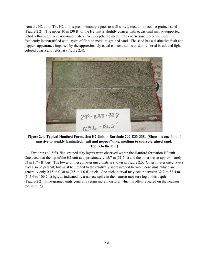
from the H2 unit. The H2 unit is predominantly a poor to well sorted, medium to coarse-grained sand (Figure 2.2). The upper 10 m (30 ft) of the H2 unit is slightly coarser with occasional matrix-supported pebbles floating in a coarse-sand matrix. With depth, the medium to coarse sand becomes more frequently interstratified with layers of fine- to medium-grained sand. The sand has a distinctive “salt and pepper” appearance imparted by the approximately equal concentrations of dark-colored basalt and light-colored quartz and feldspar (Figure 2.4).

Figure 2.4. Typical Hanford Formation H2 Unit in Borehole 299-E33-338. (Shown is one foot of

massive to weakly laminated, “salt and pepper”-like, medium to coarse-grained sand. Top is to the left.)

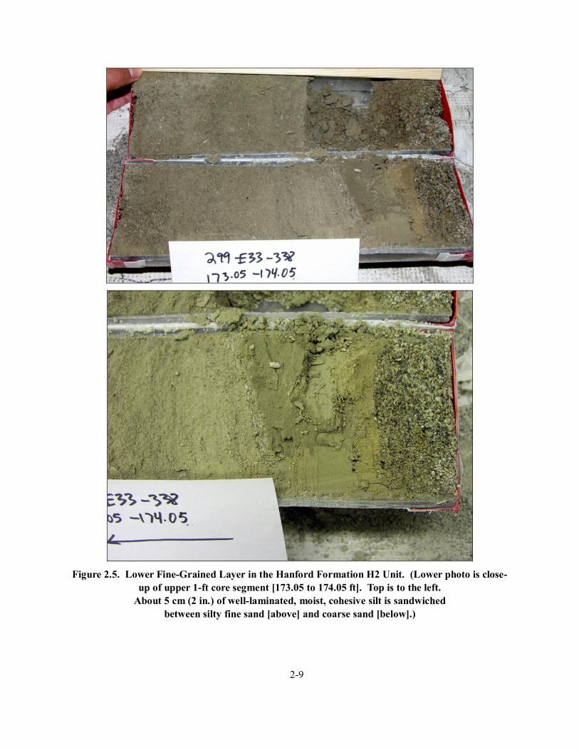
Two thin (<0.5 ft), fine-grained silty layers were observed within the Hanford formation H2 unit. One occurs at the top of the H2 unit at approximately 15.7 m (51.5 ft) and the other lies at approximately 53 m (174 ft) bgs. The lower of these fine-grained units is shown in Figure 2.5. Other fine-grained layers may also be present, but must be limited to the relatively short interval between core runs, which are generally only 0.15 to 0.30 m (0.5 to 1.0 ft) thick. One such interval may occur between 32.2 to 32.4 m (105.6 to 106.2 ft) bgs, as indicated by a narrow spike in the neutron moisture log at this depth (Figure 2.2). Fine-grained units generally retain more moisture, which is often revealed on the neutron moisture log.

2-9

Figure 2.5. Lower Fine-Grained Layer in the Hanford Formation H2 Unit. (Lower photo is close-

up of upper 1-ft core segment [173.05 to 174.05 ft]. Top is to the left. About 5 cm (2 in.) of well-laminated, moist, cohesive silt is sandwiched

between silty fine sand [above] and coarse sand [below].)

2-10

2.1.3 Hanford Formation H3 Unit

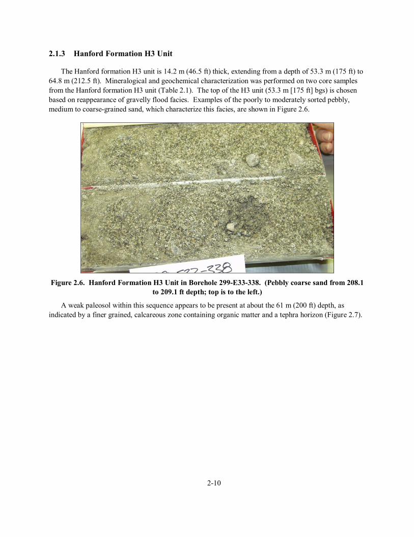
The Hanford formation H3 unit is 14.2 m (46.5 ft) thick, extending from a depth of 53.3 m (175 ft) to 64.8 m (212.5 ft). Mineralogical and geochemical characterization was performed on two core samples from the Hanford formation H3 unit (Table 2.1). The top of the H3 unit (53.3 m [175 ft] bgs) is chosen based on reappearance of gravelly flood facies. Examples of the poorly to moderately sorted pebbly, medium to coarse-grained sand, which characterize this facies, are shown in Figure 2.6.

Figure 2.6. Hanford Formation H3 Unit in Borehole 299-E33-338. (Pebbly coarse sand from 208.1

to 209.1 ft depth; top is to the left.)

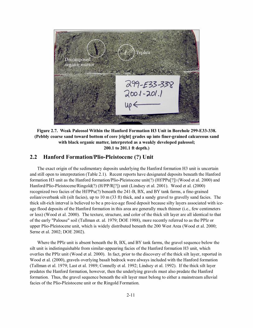
A weak paleosol within this sequence appears to be present at about the 61 m (200 ft) depth, as indicated by a finer grained, calcareous zone containing organic matter and a tephra horizon (Figure 2.7).

2-11

Figure 2.7. Weak Paleosol Within the Hanford Formation H3 Unit in Borehole 299-E33-338.

(Pebbly coarse sand toward bottom of core [right] grades up into finer-grained calcareous sand with black organic matter, interpreted as a weakly developed paleosol;

200.1 to 201.1 ft depth.)

2.2 Hanford Formation/Plio-Pleistocene (?) Unit

The exact origin of the sedimentary deposits underlying the Hanford formation H3 unit is uncertain and still open to interpretation (Table 2.1). Recent reports have designated deposits beneath the Hanford formation H3 unit as the Hanford formation/Plio-Pleistocene unit(?) (Hf/PPu[?]) (Wood et al. 2000) and Hanford/Plio-Pleistocene/Ringold(?) (H/PP/R[?]) unit (Lindsey et al. 2001). Wood et al. (2000) recognized two facies of the Hf/PPu(?) beneath the 241-B, BX, and BY tank farms, a fine-grained eolian/overbank silt (silt facies), up to 10 m (33 ft) thick, and a sandy gravel to gravelly sand facies. The thick silt-rich interval is believed to be a pre-ice-age flood deposit because silty layers associated with ice-age flood deposits of the Hanford formation in this area are generally much thinner (i.e., few centimeters or less) (Wood et al. 2000). The texture, structure, and color of the thick silt layer are all identical to that of the early "Palouse" soil (Tallman et. al. 1979; DOE 1988), more recently referred to as the PPlz or upper Plio-Pleistocene unit, which is widely distributed beneath the 200 West Area (Wood et al. 2000; Serne et al. 2002; DOE 2002).

Where the PPlz unit is absent beneath the B, BX, and BY tank farms, the gravel sequence below the silt unit is indistinguishable from similar-appearing facies of the Hanford formation H3 unit, which overlies the PPlz unit (Wood et al. 2000). In fact, prior to the discovery of the thick silt layer, reported in Wood et al. (2000), gravels overlying basalt bedrock were always included with the Hanford formation (Tallman et al. 1979; Last et al. 1989; Connelly et al. 1992; Lindsey et al. 1992). If the thick silt layer predates the Hanford formation, however, then the underlying gravels must also predate the Hanford formation. Thus, the gravel sequence beneath the silt layer must belong to either a mainstream alluvial facies of the Plio-Pleistocene unit or the Ringold Formation.

2-12

2.2.1 Silt-Dominated Facies (PPlz)

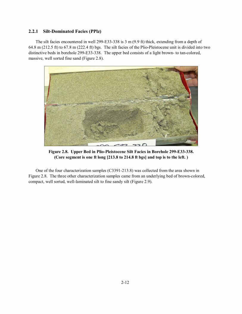
The silt facies encountered in well 299-E33-338 is 3 m (9.9 ft) thick, extending from a depth of 64.8 m (212.5 ft) to 67.8 m (222.4 ft) bgs. The silt facies of the Plio-Pleistocene unit is divided into two distinctive beds in borehole 299-E33-338. The upper bed consists of a light brown- to tan-colored, massive, well sorted fine sand (Figure 2.8).

Figure 2.8. Upper Bed in Plio-Pleistocene Silt Facies in Borehole 299-E33-338.

(Core segment is one ft long [213.8 to 214.8 ft bgs] and top is to the left. )

One of the four characterization samples (C3391-213.8) was collected from the area shown in

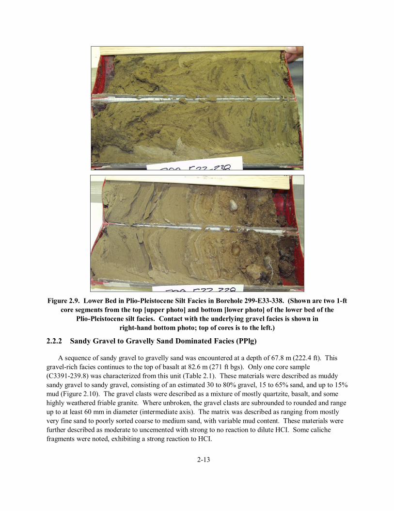
Figure 2.8. The three other characterization samples came from an underlying bed of brown-colored, compact, well sorted, well-laminated silt to fine sandy silt (Figure 2.9).

2-13

Figure 2.9. Lower Bed in Plio-Pleistocene Silt Facies in Borehole 299-E33-338. (Shown are two 1-ft

core segments from the top [upper photo] and bottom [lower photo] of the lower bed of the Plio-Pleistocene silt facies. Contact with the underlying gravel facies is shown in

right-hand bottom photo; top of cores is to the left.)

2.2.2 Sandy Gravel to Gravelly Sand Dominated Facies (PPlg)

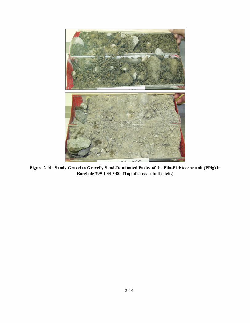
A sequence of sandy gravel to gravelly sand was encountered at a depth of 67.8 m (222.4 ft). This gravel-rich facies continues to the top of basalt at 82.6 m (271 ft bgs). Only one core sample (C3391-239.8) was characterized from this unit (Table 2.1). These materials were described as muddy sandy gravel to sandy gravel, consisting of an estimated 30 to 80% gravel, 15 to 65% sand, and up to 15% mud (Figure 2.10). The gravel clasts were described as a mixture of mostly quartzite, basalt, and some highly weathered friable granite. Where unbroken, the gravel clasts are subrounded to rounded and range up to at least 60 mm in diameter (intermediate axis). The matrix was described as ranging from mostly very fine sand to poorly sorted coarse to medium sand, with variable mud content. These materials were further described as moderate to uncemented with strong to no reaction to dilute HCI. Some caliche fragments were noted, exhibiting a strong reaction to HCI.

2-14

Figure 2.10. Sandy Gravel to Gravelly Sand-Dominated Facies of the Plio-Pleistocene unit (PPlg) in

Borehole 299-E33-338. (Top of cores is to the left.)

3-1

3.0 Characterization Analytical Methods

This section discusses the methods and procedure used to determine which samples would be characterized and which parameters would be measured.

3.1 Geochemical and Analytical Laboratory Methods and Materials

Geochemical and analytical methods used in the laboratory to characterize the core sediment samples are discussed in this section. Physical properties analyzed include mass water content, particle size distribution, and sand/silt/clay percentages. A variety of geochemical techniques were performed on the sediments including elemental analysis by fusion, 1:1 sediment to water extraction, and 8M nitric acid extraction. Mineralogical analyses were performed using x-ray diffraction (XRD).

3.1.1 Borehole Core Sampling

The samples characterized from RCRA borehole 299-E33-338 were obtained during the geologic description process immediately upon opening the sealed liners in the same fashion as described in the report Characterization of Vadose Zone Sediments: Uncontaminated RCRA Borehole Core Samples and Composite Samples (Serne et. al. 2002). As before, the split-spoon samples were obtained in clear, plastic Lexan liners that were 12 in. long and 4 in. in diameter. Plastic end caps were removed, and the liners were cut down both sides with a circular saw. The core was opened in a fashion similar to opening a clam shell, facilitated by the relatively unconsolidated nature of the sediment. The two halves of the liner were laid on a table and quickly photographed and sub-sampled to avoid excessive loss of moisture. Small aliquots were removed in an attempt to construct a representative sample for the entire sleeve. Depending on the sample matrix, very coarse pebble and larger material (i.e., >32 mm) was avoided during sub-sampling. Larger substrate was excluded to provide moisture contents representative of counting and 1:1 sediment-to-water extract samples. Results from sub-sample measurements should then take into consideration a possible bias toward higher concentrations for some analytes that are associated with smaller sized sediment fractions. The sediment in the Plio-Pleistocene silt-dominated facies contained no large pebbles or cobbles.

When distinct contacts were observed in a core sample, the sampling was performed separately on the different lithologies. After sampling and the geologic descriptions were completed, the two halves of the liner were reassembled and retaped to prevent further disturbance or loss of moisture. Liners were then returned to refrigerated storage in the dark at 4oC.

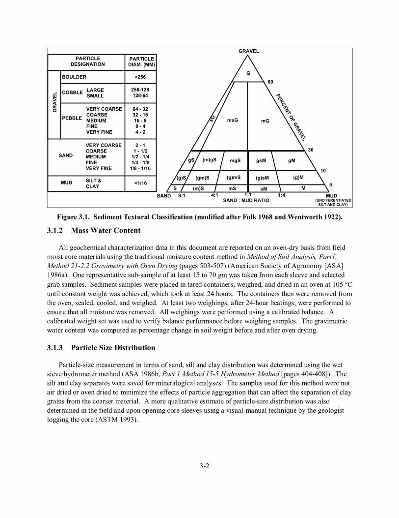
Procedures ASTM D2488-93 (ASTM 1993) and accepted PNNL laboratory procedure for groundwater investigation were followed for visual descriptions and geologic description of all split-spoon samples. The sediment classification scheme used for geologic identification of the sediment types is based on the modified Folk (1968) and/or Wentworth (1922) classification scheme (Figure 3.1). However, the mineralogic and geochemical characterization relied on further separation of the mud into discrete silt and clay sizes. The selected Lexan liners from borehole 299-E33-338 were sub-sampled using stainless steel spatulas. The depths and corresponding stratigraphic unit designations are shown in Table 2.1. In most cases, field moist sediment was used to measure the various parameters discussed in Section 4.0, but the results are on an oven dry-weight basis.

3-2

PARTICLE DESIGNATION

PARTICLE DIAM. (MM)

BOULDER

COBBLE LARGE SMALL

256-128 128-64

VERY COARSE COARSE MEDIUM FINE VERY FINE

VERY COARSE COARSE MEDIUM FINE VERY FINE

PEBBLE

SAND

MUD SILT & CLAY

GR

AVE

L

64 - 32 32 - 16 16 - 8 8 - 4 4 - 2

2 - 1 1 - 1/2

1/2 - 1/4 1/4 - 1/8

1/8 - 1/16

<1/16

>256

(UNDIFERENTIATED

5

80

30

10

GRAVEL

G

SAND MUD9:1 4:1 1:1 1:4

sG msG mG

SILT AND CLAY)

PERCENT OF GRAVEL

SAND : MUD RATIO

gS (m)gS mgS gsM gM

(g)S (gm)S (g)mS (g)sM (g)M

S (m)S mS sM M

Figure 3.1. Sediment Textural Classification (modified after Folk 1968 and Wentworth 1922).

3.1.2 Mass Water Content

All geochemical characterization data in this document are reported on an oven-dry basis from field moist core materials using the traditional moisture content method in Method of Soil Analysis, Part1, Method 21-2.2 Gravimetry with Oven Drying (pages 503-507) (American Society of Agronomy [ASA] 1986a). One representative sub-sample of at least 15 to 70 gm was taken from each sleeve and selected grab samples. Sediment samples were placed in tared containers, weighed, and dried in an oven at 105 °C until constant weight was achieved, which took at least 24 hours. The containers then were removed from the oven, sealed, cooled, and weighed. At least two weighings, after 24-hour heatings, were performed to ensure that all moisture was removed. All weighings were performed using a calibrated balance. A calibrated weight set was used to verify balance performance before weighing samples. The gravimetric water content was computed as percentage change in soil weight before and after oven drying.

3.1.3 Particle Size Distribution

Particle-size measurement in terms of sand, silt and clay distribution was determined using the wet sieve/hydrometer method (ASA 1986b, Part 1 Method 15-5 Hydrometer Method [pages 404-408]). The silt and clay separates were saved for mineralogical analyses. The samples used for this method were not air dried or oven dried to minimize the effects of particle aggregation that can affect the separation of clay grains from the coarser material. A more qualitative estimate of particle-size distribution was also determined in the field and upon opening core sleeves using a visual-manual technique by the geologist logging the core (ASTM 1993).

3-3

3.1.4 Particle Density

The particle density of bulk grains was determined using pychnometers (ASA 1986c, Part 1; Method 14-3 Pychnometer Method [pages 378-379] on oven-dried material.

3.1.5 1:1 Sediment-to-Water Extract

The water-soluble inorganic constituents were determined using a 1:1 by weight sediment-to-deionized water extract method. This method was chosen because the sediment was too dry to easily extract vadose zone porewater. The extracts were prepared by adding an exact weight of deionized water to approximately 60 to 80 gm of sediment sub-sampled from each sleeve and selected grab samples. The weight of deionized water needed was calculated based on the weight of the field-moist samples and their previously determined moisture contents. The sum of the existing moisture (porewater) and the deionized water was fixed at the mass of the dry sediment. The appropriate amount of deionized water was added to screw cap jars containing the sediment samples. The jars were sealed and briefly shaken by hand, then placed on a mechanical orbital shaker for 1 hour. The samples were allowed to settle until the supernatant liquid was fairly clear. The supernatant was carefully decanted and separated into unfiltered aliquots for conductivity and pH determinations, and filtered aliquots (passed through 0.45 µm membranes) for anion, cation, carbon, and radionuclide analyses. More details can be found in Rhoades (1996) within Methods of Soils Analysis Part 3 (ASA 1996).

3.1.6 8 M Nitric Acid Extract

Approximately 20 grams of oven-dried sediment was contacted with 8 M nitric acid at a ratio of approximately 5 parts acid to 1 part sediment. The slurries were heated to approximately 80 °C for several hours and then the fluid was separated by centrifugation and filtration through 0.2 µm membranes. The acid extracts were analyzed for major cations and trace metals using inductively coupled plasma (ICP) unit and inductively coupled plasma – mass spectrometer (ICP-MS) techniques, respectively. The acid digestion procedure is based on U.S. Environmental Protection Agency (EPA) SW-846 Method 3050B (EPA 2000a) that can be accessed on-line at http://www.epa.gov/epaoswer/hazwaste/test/sw846.htm.

3.1.7 pH and Conductivity

Two approximately 3-ml, aliquots of the unfiltered 1:1 by weight sediment-to-water extract supernatant were used for pH and conductivity measurements. The pH values for the extracts were measured with a solid-state pH electrode and a pH meter calibrated with buffers 4, 7, and 10. Conductivity was measured and compared to potassium chloride standards with a range of 0.001 M to 1.0 M.

3.1.8 Anion Analysis

The 1:1 sediment-to-water extracts were analyzed for anions using an ion chromatograph. Fluoride, acetate, formate, chloride, nitrite, bromide, nitrate, carbonate, phosphate, sulfate, and oxalate were separated on a Dionex AS17 column with a gradient elution of 1 mM to 35 mM NaOH and measured

3-4

using a conductivity detector. This methodology is based on EPA Method 300.0A (EPA 1984) with the exception of using the gradient elution of sodium hydroxide.

3.1.9 Cations and Trace Metals

Major cation analysis was performed with an ICP unit using high-purity calibration standards to generate calibration curves and verify continuing calibration during the analysis run. Dilutions of 100x, 50x, 10x, and 5x were made of each sample for analysis to investigate and correct for matrix interferences. Details are found in EPA Method 6010B (EPA 2000b). The second instrument used to analyze trace metals, including technetium-99 and uranium-238, was an ICP-MS using accepted PNNL procedures similar to EPA Method 6020 (EPA 2000c).

3.1.10 Alkalinity

The alkalinity content of several of the 1:1 sediment-to-water extracts were measured using standard titration with acid and a carbon analyzer. The alkalinity procedure is equivalent to the U.S. Geological Survey Method Field Manual (USGS 2001) http://water.usgs.gov/owq.

3.1.11 Carbon Content

The carbon contents of borehole sediment samples were determined using ASTM Method D4129-88, Standard Methods for Total and Organic Carbon in Water Oxidation by High Temperature Oxidation and by Coulometric Detection (ASTM 1988). Total carbon in all samples was determined using a Coulometrics, Inc. Model 5051 Carbon Dioxide Coulometer with combustion at approximately 980°C. Ultrapure oxygen was used to sweep the combustion products through a barium chromate catalyst tube for conversion to carbon dioxide. Evolved carbon dioxide was quantified through coulometric titration following absorption in a solution containing ethanolamine. Equipment output reported carbon content values in micrograms per sample. Soil samples for determining total carbon content were placed into pre-combusted, tared, platinum combustion boats and weighed on a four-place analytical balance. After the combustion boats were placed into the furnace introduction tube, a 1-minute waiting period was allowed so that the ultrapure oxygen carrier gas could remove any carbon dioxide introduced to the system from the atmosphere during sample placement. After this system sparge, the sample was moved into the combustion furnace and titration begun. Sample titration readings were performed at 3 minutes after combustion began and again once stability was reached, usually within the next 2 minutes. The system background was determined by performing the entire process using an empty, pre-combusted, platinum boat. Adequate system performance was confirmed by analyzing for known quantities of a calcium carbonate standard.

Inorganic carbon contents for borehole sediment samples were determined using a Coulometrics, Inc., Model 5051 Carbon Dioxide Coulometer. Soil samples were weighed on a four-place analytical balance, then placed into acid-treated glass tubes. Following placement of sample tubes into the system, a 1-minute waiting period allowed the ultrapure oxygen carrier gas to remove any carbon dioxide introduced to the system from the atmosphere. Inorganic carbon was released through acid-assisted evolution (3M hydrochloric acid) with heating to 80 °C. Samples were completely covered by the acid to allow full reaction to occur. Ultrapure oxygen gas swept the resultant carbon dioxide through the

3-5

equipment to determine inorganic carbon content by coulometric titration. Sample titration readings were performed 5 minutes following acid addition and again once stability was reached, usually within 10 minutes. Known quantities of calcium carbonate standards were analyzed to verify that the equipment was operating properly. Background values were determined. Inorganic carbon content was determined through calculations performed using the microgram per-sample output data and sample weights. Organic carbon was calculated by subtracting inorganic carbon from total carbon and using the remainder.

3.1.12 Bulk Elemental Analysis

Samples were mixed with a flux of lithium metaborate and lithium tetraborate and fused in an induction furnace. The molten melt was immediately poured into a solution of 5% nitric acid containing an internal standard, and mixed continuously until completely dissolved (approximately 30 minutes). The samples were run for major oxides and selected trace elements on a combination simultaneous/sequential Thermo Jarrell-Ash ENVRO II ICP and a Perkin Elmer SCIEX ELAN 6000 ICP-MS. Calibration was performed using USGS and Canmet certified reference materials.

3.1.13 Mineralogy

The mineralogies of the bulk sample and silt- and clay-sized fractions of selected sediment samples were determined by XRD techniques. Bulk sediment samples were dispersed by transferring 100 gm of sediment into a 1-liter bottle and mixing with 1 liter of 0.001 M solution of sodium hexametaphosphate (a dispersant). The suspensions were allowed to shake overnight to ensure complete dispersion. The sand fraction was separated from the dispersed sample by wet sieving through a #230 sieve. The silt fractions were separated from the clay fractions by using Stoke’s settling law described in Jackson (1969). The lower limit of the fraction was taken at >2 microns. Sand and silt fractions were oven dried at 110°C and prepared for XRD.

Each clay suspension was concentrated to an approximate volume of 10 ml by adding a few drops of 10 N magnesium chloride to the dispersing solution. Concentrations of the clay in the concentrated suspensions were determined by drying known volumes and weighing the dried sediment. The density of the slurry was calculated from the volume pipetted and the final weight of dried sediment. Volumes of slurry equaling 250 mg of clay were transferred into centrifuge tubes and treated to remove carbonates following the procedure described by Jackson (1969). The carbonate free clay was then saturated with either magnesium (Mg2+) or potassium (K+) cations. Clay samples were prepared using the Drever (1973) method and placed onto an aluminum slide for XRD analysis. Due to the tendency of the clay film to peel and curl, the magnesium (Mg2+)-saturated specimens were solvated with a few drops of a 10% solution of ethylene glycol in ethanol and placed into a desiccator containing excess ethylene glycol for a minimum of 24 hours. Potassium-saturated slides were air dried and analyzed, then heated to 575°C and reanalyzed.

All samples were analyzed on a Scintag x-ray diffraction unit equipped with a Pelter thermoelectrically cooled detector and a copper x-ray tube. Slides of preferentially oriented clay were scanned from 2 to 45 degrees 2θ, and randomly oriented powder mounts were scanned from 2 to 75 degrees 2θ. The bulk samples were prepared by crushing approximately 0.5 gm of sample to a fine

3-6

powder that was then packed into a small circular holder. After air drying approximately 0.5 gm of the clay slurry, a random mount was prepared and analyzed from 2 to 75° 2θ.

Semiquantification of mineral phases by XRD was performed according to Brindley and Brown (1980). The relationship of intensity and mass absorption to the weight fraction of an unknown phase is expressed as:

I/Ip=µp/µ (wf) where:

I is the intensity of the unknown phase Ip is the intensity of the pure phase µp is the mass absorption of the pure phase µ is the average mass absorption of the unknown mixture wf is the weight fraction of the unknown.

Pure mineral phases of illite, smectite, kaolinite, and chlorite were obtained from the Clay Mineral Society’s source clays repository (operated from the University of Missouri in Columbia), and analyzed under the same conditions as the sediment samples. Quartz, feldspars, and calcite standards were purchased from the Excalibur Mineral Company (Peekskill, New York), ground, and analyzed on the diffractometer to obtain intensities for pure nonclay phases.

The mass attenuation coefficients of selected samples were measured according to Brindley and Brown (1980). Ground bulk powders and air-dried clays were packed into a 2.39-cm (0.94-in.) thick circular holder with no backing. The holder was placed in front of the detector and positioned to allow the x-ray beam, diffracted from pure quartz, to pass through the sample and into the detector. The scan was analyzed from 26 to 27 degrees 2θ. The mass attenuation coefficients were measured directly using the following equation:

µ= (1/ρx)ln(Io/Ix) where:

1/ρx is the mass per unit area as the sample is prepared Io is the intensity of the incident beam Ix is the intensity of the transmitted beam through sample thickness x.

In addition to x-ray diffraction, transmission electron microscopy (TEM) characterization of selected

samples was conducted on a JEOL 1200X electron microscope equipped with a Links detector system. Samples were prepared for TEM by transferring a small aliquot of a dilute clay slurry onto a formvar carbon coated 3-ml copper support grid. The clay solution contained 0.15% tert-butylamine to reduce the surface tension of water.

Structural formulas were derived from data collected from the TEM analysis. On average, an energy dispersive x-ray spectra was collected from a minimum of five particles from the same mineral phase common to the sample. The x-ray spectra were collected and processed using the Cliff-Lorimer Ratio Thin Section method and then converted to a structural formula [based on half-unit cell (O10(OH)2) described in Moore and Reynolds (1989) and Newman (1987)].

3-7

3.1.14 Water Potential (Suction) Measurements

Suction measurements were made on most of the core liners and grab samples from the borehole using PNNL’s filter paper method. This method relies on the use of a sandwich of three filter papers that rapidly equilibrates with the sediment sample. The middle filter paper does not contact sediment that might stick to the paper and bias the mass measurements. At equilibrium, the matric suction in the filter paper is the same as the matric suction of the sediment sample. The dry filter paper sandwiches were placed in the airtight liners or grab sample jars while still filled with the sediment for at least 3 to 12 weeks to allow sufficient time for the matric suction in the sediment to equilibrate with the matric suction in the filter paper. The mass of the wetted middle filter paper that had no direct contact with the sediment was subsequently determined, and the suction of the sediment was determined from a calibration relationship between filter paper water content and matric suction.

The relationships used for converting the water content of filter paper to matric suction for Whatman #42 filter paper have been determined by Deka et al. (1995) and can be expressed as:

Sm = 10(5.144 - 6.699 w)/10 for w < 0.5 Sm = 10(2.383 - 1.309 w)/10 for w >0.5

where: Sm is the matric suction (m) and w is the gravimetric water content (g/g).

One hundred eighty-eight samples from borehole 299-E33-338 were analyzed for water content and soil matric suction. The samples covered the entire borehole profile from 9.6 to 253.6 ft (2.93 to 77.3 m) bgs.

4-1

4.0 Analytical Results for Sediment Samples

This section discusses the analytical results for the core samples from borehole 299-E33-338.

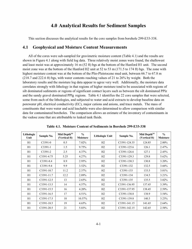
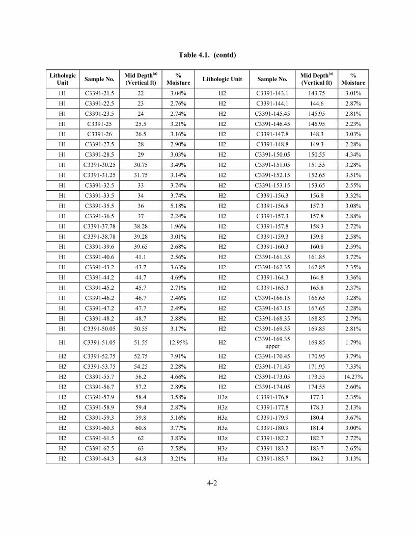
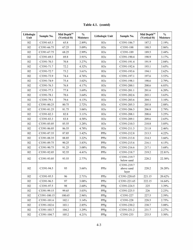
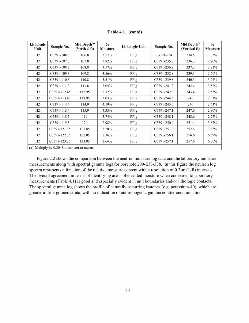
4.1 Geophysical and Moisture Content Measurements

All of the cores were sub-sampled for gravimetric moisture content (Table 4.1) and the results are shown in Figure 4.1 along with field log data. Three relatively moist zones were found, the shallowest and least moist was at approximately 16 m (52 ft) bgs at the bottom of the Hanford H1 unit. The second moist zone was at the bottom of the Hanford H2 unit at 52 to 53 m (171.5 to 174 ft) bgs. The zone with highest moisture content was at the bottom of the Plio-Pleistocene mud unit, between 66.7 to 67.8 m (218.7 and 222.6 ft) bgs, with water contents reaching values of 21 to 26% by weight. Both the laboratory results and the moisture log data appear to agree very well. Additionally, the moisture data correlates strongly with lithology in that regions of higher moisture tend to be associated with regions of silt dominated sediments or regions of significant contact layers such as between the silt dominated PPlz and the sandy gravel dominated PPlg regions. Table 4.1 identifies the 22 core samples that were selected, some from each of the lithologies, and subjected to water and acid extracts to develop baseline data on porewater pH, electrical conductivity (EC), major cations and anions, and trace metals. The mass of constituents that were water and acid leachable were also determined to allow comparison with similar data for contaminated boreholes. The comparison allows an estimate of the inventory of contaminants in the vadose zone that are attributable to leaked tank fluids.

Table 4.1. Moisture Content of Sediments in Borehole 299-E33-338

Lithologic Unit Sample No. Mid Depth(a)

(Vertical ft) %

Moisture Lithologic Unit Sample No. Mid Depth(a) (Vertical ft)

% Moisture

H1 C3391-0 0.5 7.02% H2 C3391-124.35 124.85 2.00% H1 C3391-1 1.5 9.75% H2 C3391-125.6 126.1 2.47% H1 C3391-2 2.5 4.37% H2 C3391-126.6 127.1 2.45% H1 C3391-4.75 5.25 4.27% H2 C3391-129.3 129.8 5.62% H1 C3391-8.4 8.9 2.95% H2 C3391-130.3 130.8 3.20% H1 C3391-9.4 9.9 3.52% H2 C3391-132 132.5 3.66% H1 C3391-10.7 11.2 2.37% H2 C3391-133 133.5 3.01% H1 C3391-11.7 12.2 2.89% H2 C3391-134 134.5 3.21% H1 C3391-12.5 13 2.65% H2 C3391-135 135.5 3.02% H1 C3391-13.5 14 4.57% H2 C3391-136.95 137.45 3.39% H1 C3391-15.5 16 4.20% H2 C3391-137.95 138.45 2.59% H1 C3391-16.5 17 4.51% H2 C3391-138.8 138.9 3.54% H1 C3391-17.5 18 10.57% H2 C3391-139.8 140.3 3.23% H1 C3391-18.5 19 4.65% H2 C3391-141.15 141.65 2.64% H1 C3391-20.5 21 5.03% H2 C3391-142.15 142.65 2.58%

4-2

Table 4.1. (contd)

Lithologic Unit Sample No. Mid Depth(a)

(Vertical ft) %

Moisture Lithologic Unit Sample No. Mid Depth(a) (Vertical ft)

% Moisture

H1 C3391-21.5 22 3.04% H2 C3391-143.1 143.75 3.01%

H1 C3391-22.5 23 2.76% H2 C3391-144.1 144.6 2.87%

H1 C3391-23.5 24 2.74% H2 C3391-145.45 145.95 2.81%

H1 C3391-25 25.5 3.21% H2 C3391-146.45 146.95 2.23% H1 C3391-26 26.5 3.16% H2 C3391-147.8 148.3 3.03%

H1 C3391-27.5 28 2.90% H2 C3391-148.8 149.3 2.28%

H1 C3391-28.5 29 3.03% H2 C3391-150.05 150.55 4.34%

H1 C3391-30.25 30.75 3.49% H2 C3391-151.05 151.55 3.28%

H1 C3391-31.25 31.75 3.14% H2 C3391-152.15 152.65 3.51%

H1 C3391-32.5 33 3.74% H2 C3391-153.15 153.65 2.55%

H1 C3391-33.5 34 3.74% H2 C3391-156.3 156.8 3.32%

H1 C3391-35.5 36 5.18% H2 C3391-156.8 157.3 3.08%

H1 C3391-36.5 37 2.24% H2 C3391-157.3 157.8 2.88%

H1 C3391-37.78 38.28 1.96% H2 C3391-157.8 158.3 2.72%

H1 C3391-38.78 39.28 3.01% H2 C3391-159.3 159.8 2.58% H1 C3391-39.6 39.65 2.68% H2 C3391-160.3 160.8 2.59%

H1 C3391-40.6 41.1 2.56% H2 C3391-161.35 161.85 3.72%

H1 C3391-43.2 43.7 3.63% H2 C3391-162.35 162.85 2.35%

H1 C3391-44.2 44.7 4.69% H2 C3391-164.3 164.8 3.36%

H1 C3391-45.2 45.7 2.71% H2 C3391-165.3 165.8 2.37%

H1 C3391-46.2 46.7 2.46% H2 C3391-166.15 166.65 3.28%

H1 C3391-47.2 47.7 2.49% H2 C3391-167.15 167.65 2.28%

H1 C3391-48.2 48.7 2.88% H2 C3391-168.35 168.85 2.79%

H1 C3391-50.05 50.55 3.17% H2 C3391-169.35 169.85 2.81%

H1 C3391-51.05 51.55 12.95% H2 C3391-169.35 upper 169.85 1.79%

H2 C3391-52.75 52.75 7.91% H2 C3391-170.45 170.95 3.79%

H2 C3391-53.75 54.25 2.28% H2 C3391-171.45 171.95 7.33%

H2 C3391-55.7 56.2 4.66% H2 C3391-173.05 173.55 14.27% H2 C3391-56.7 57.2 2.89% H2 C3391-174.05 174.55 2.60%

H2 C3391-57.9 58.4 3.58% H3z C3391-176.8 177.3 2.35%

H2 C3391-58.9 59.4 2.87% H3z C3391-177.8 178.3 2.13%

H2 C3391-59.3 59.8 5.16% H3z C3391-179.9 180.4 3.67%

H2 C3391-60.3 60.8 3.77% H3z C3391-180.9 181.4 3.00%

H2 C3391-61.5 62 3.83% H3z C3391-182.2 182.7 2.72%

H2 C3391-62.5 63 2.58% H3z C3391-183.2 183.7 2.65%

H2 C3391-64.3 64.8 3.21% H3z C3391-185.7 186.2 3.13%

4-3

Table 4.1. (contd)

Lithologic Unit Sample No. Mid Depth(a)

(Vertical ft) %

Moisture Lithologic Unit Sample No. Mid Depth(a) (Vertical ft)

% Moisture

H2 C3391-65.3 65.8 2.89% H3z C3391-186.7 187.2 2.19%

H2 C3391-66.75 67.25 5.09% H3z C3391-188 188.5 2.86%

H2 C3391-67.75 68.25 2.99% H3z C3391-189 189.5 2.44%

H2 C3391-69.3 69.8 3.91% H3z C3391-190.4 190.9 3.17%

H2 C3391-70.3 70.8 3.27% H3z C3391-191.4 191.9 2.84%

H2 C3391-71.7 72.2 4.32% H3z C3391-192.6 193.1 3.65%

H2 C3391-72.7 73.2 3.61% H3z C3391-193.6 194.1 2.62%

H2 C3391-73.9 74.4 4.76% H3z C3391-197.1 197.6 3.53%

H2 C3391-74.9 75.4 3.02% H3z C3391-198.1 198.6 2.79% H2 C3391-76.3 76.8 4.17% H3z C3391-200.1 200.6 6.03%

H2 C3391-77.3 77.8 3.69% H3z C3391-201.1 201.6 6.20%

H2 C3391-78.1 78.6 3.64% H3z C3391-202.6 203.1 3.63%

H2 C3391-79.1 79.6 4.13% H3z C3391-203.6 204.1 3.10%

H2 C3391-80.25 80.75 2.72% H3z C3391-205.3 205.8 2.88%

H2 C3391-81.25 81.75 3.06% H3z C3391-206.3 206.8 2.79%

H2 C3391-82.3 82.8 3.11% H3z C3391-208.1 208.6 3.25%

H2 C3391-83.3 83.8 4.58% H3z C3391-209.1 209.6 2.65%

H2 C3391-85.05 85.55 3.28% H3z C3391-210.3 210.8 3.05%

H2 C3391-86.05 86.55 4.78% H3z C3391-211.3 211.8 2.46%

H2 C3391-87.35 87.85 3.42% PPlz C3391-212.8 213.3 4.22%

H2 C3391-88.35 88.85 3.22% PPlz C3391-213.8 214.3 3.66% H2 C3391-89.75 90.25 3.83% PPlz C3391-215.6 216.1 4.15%

H2 C3391-90.75 91.25 3.08% PPlz C3391-216.6 217.1 3.68%

H2 C3391-92.05 92.55 4.41% PPlz C3391-218.7 219.2 22.81%

H2 C3391-93.05 93.55 2.77% PPlz C3391-219.7 below sand 220.2 22.30%

H2 C3391-94.5 95 3.66% PPlz C3391-219.7 above sand

layer 220.2 26.20%

H2 C3391-95.5 96 2.71% PPlz C3391-220.65 221.15 20.62%

H2 C3391-96.5 97 3.08% PPlz C3391-221.65 222.15 16.64%

H2 C3391-97.5 98 2.60% PPlg C3391-224.5 225 3.39%

H2 C3391-99.15 99.65 3.03% PPlg C3391-225.5 226 2.23%

H2 C3391-100.15 100.65 2.96% PPlg C3391-227 227.5 2.59%

H2 C3391-101.6 102.1 3.14% PPlg C3391-228 228.5 2.75%

H2 C3391-102.6 103.1 2.85% PPlg C3391-230.2 230.7 3.08%

H2 C3391-103.7 104.2 3.29% PPlg C3391-231.2 231.7 2.27%

H2 C3391-104.7 105.2 4.21% PPlg C3391-233 233.5 3.50%

4-4

Table 4.1. (contd)

Lithologic Unit Sample No. Mid Depth(a)

(Vertical ft) %

Moisture Lithologic Unit Sample No. Mid Depth(a) (Vertical ft)

% Moisture

H2 C3391-106.3 106.8 3.57% PPlg C3391-234 234.5 3.03%

H2 C3391-107.3 107.8 3.82% PPlg C3391-235.8 236.3 2.20%

H2 C3391-108.3 108.8 3.57% PPlg C3391-236.8 237.3 2.81%

H2 C3391-109.3 109.8 3.56% PPlg C3391-238.8 239.3 2.60%

H2 C3391-110.3 110.8 3.51% PPlg C3391-239.8 240.3 3.27%

H2 C3391-111.3 111.8 3.05% PPlg C3391-241.9 242.4 3.52%

H2 C3391-112.45 112.95 3.72% PPlg C3391-242.9 243.4 2.55%

H2 C3391-113.45 113.95 3.03% PPlg C3391-244.5 245 2.51%

H2 C3391-114.4 114.9 4.19% PPlg C3391-245.5 246 2.64% H2 C3391-115.4 115.9 3.35% PPlg C3391-247.1 247.6 2.80%

H2 C3391-118.5 119 5.74% PPlg C3391-248.1 248.6 2.77%

H2 C3391-119.5 120 2.98% PPlg C3391-250.9 251.4 3.87%

H2 C3391-121.35 121.85 3.20% PPlg C3391-251.9 252.4 3.35%

H2 C3391-122.35 122.85 2.36% PPlg C3391-256.1 256.6 6.59%

H2 C3391-123.35 123.85 2.66% PPlg C3391-257.1 257.6 6.80%

(a) Multiply by 0.3048 to convert to meters.

Figure 2.2 shows the comparison between the neutron moisture log data and the laboratory moisture

measurements along with spectral gamma logs for borehole 299-E33-338. In this figure the neutron log spectra represents a function of the relative moisture content with a resolution of 0.3-m (1-ft) intervals. The overall agreement in terms of identifying areas of elevated moisture when compared to laboratory measurements (Table 4.1) is good and especially evident in unit boundaries and/or lithologic contacts. The spectral gamma log shows the profile of naturally occurring isotopes (e.g. potassium-40), which are greater in fine-grained strata, with no indication of anthropogenic gamma emitter contamination.

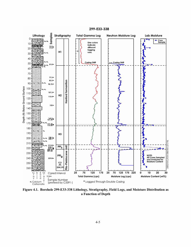
4-5

Figure 4.1. Borehole 299-E33-338 Lithology, Stratigraphy, Field Logs, and Moisture Distribution as

a Function of Depth

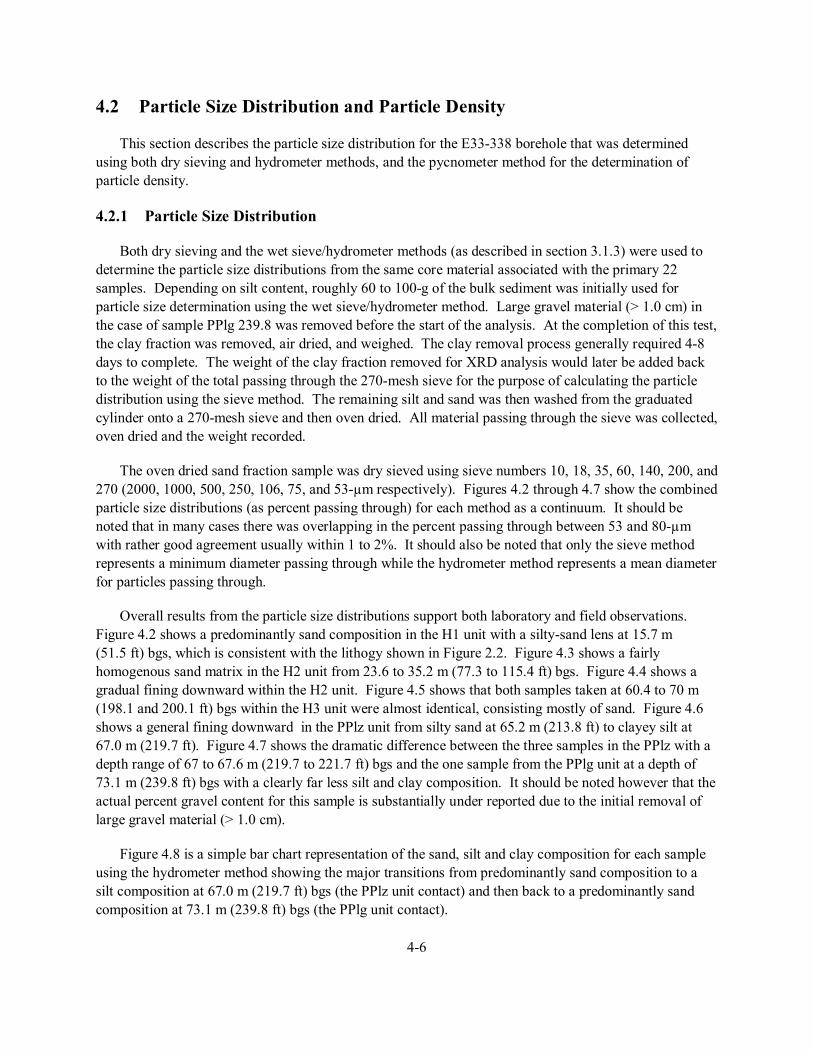
4-6

4.2 Particle Size Distribution and Particle Density

This section describes the particle size distribution for the E33-338 borehole that was determined using both dry sieving and hydrometer methods, and the pycnometer method for the determination of particle density.

4.2.1 Particle Size Distribution

Both dry sieving and the wet sieve/hydrometer methods (as described in section 3.1.3) were used to determine the particle size distributions from the same core material associated with the primary 22 samples. Depending on silt content, roughly 60 to 100-g of the bulk sediment was initially used for particle size determination using the wet sieve/hydrometer method. Large gravel material (> 1.0 cm) in the case of sample PPlg 239.8 was removed before the start of the analysis. At the completion of this test, the clay fraction was removed, air dried, and weighed. The clay removal process generally required 4-8 days to complete. The weight of the clay fraction removed for XRD analysis would later be added back to the weight of the total passing through the 270-mesh sieve for the purpose of calculating the particle distribution using the sieve method. The remaining silt and sand was then washed from the graduated cylinder onto a 270-mesh sieve and then oven dried. All material passing through the sieve was collected, oven dried and the weight recorded.

The oven dried sand fraction sample was dry sieved using sieve numbers 10, 18, 35, 60, 140, 200, and 270 (2000, 1000, 500, 250, 106, 75, and 53-µm respectively). Figures 4.2 through 4.7 show the combined particle size distributions (as percent passing through) for each method as a continuum. It should be noted that in many cases there was overlapping in the percent passing through between 53 and 80-µm with rather good agreement usually within 1 to 2%. It should also be noted that only the sieve method represents a minimum diameter passing through while the hydrometer method represents a mean diameter for particles passing through.

Overall results from the particle size distributions support both laboratory and field observations. Figure 4.2 shows a predominantly sand composition in the H1 unit with a silty-sand lens at 15.7 m (51.5 ft) bgs, which is consistent with the lithogy shown in Figure 2.2. Figure 4.3 shows a fairly homogenous sand matrix in the H2 unit from 23.6 to 35.2 m (77.3 to 115.4 ft) bgs. Figure 4.4 shows a gradual fining downward within the H2 unit. Figure 4.5 shows that both samples taken at 60.4 to 70 m (198.1 and 200.1 ft) bgs within the H3 unit were almost identical, consisting mostly of sand. Figure 4.6 shows a general fining downward in the PPlz unit from silty sand at 65.2 m (213.8 ft) to clayey silt at 67.0 m (219.7 ft). Figure 4.7 shows the dramatic difference between the three samples in the PPlz with a depth range of 67 to 67.6 m (219.7 to 221.7 ft) bgs and the one sample from the PPlg unit at a depth of 73.1 m (239.8 ft) bgs with a clearly far less silt and clay composition. It should be noted however that the actual percent gravel content for this sample is substantially under reported due to the initial removal of large gravel material (> 1.0 cm).

Figure 4.8 is a simple bar chart representation of the sand, silt and clay composition for each sample using the hydrometer method showing the major transitions from predominantly sand composition to a silt composition at 67.0 m (219.7 ft) bgs (the PPlz unit contact) and then back to a predominantly sand composition at 73.1 m (239.8 ft) bgs (the PPlg unit contact).

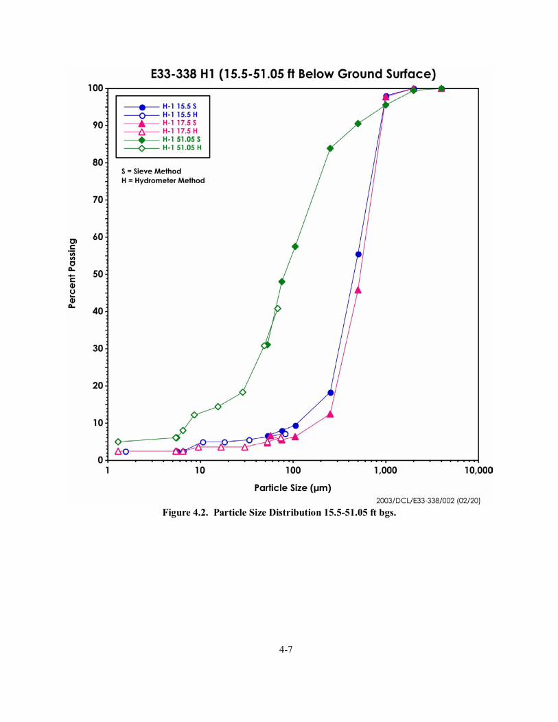
4-7

Figure 4.2. Particle Size Distribution 15.5-51.05 ft bgs.

4-8

Figure 4.3. Particle Size Distribution 77.3-115.4 ft bgs.

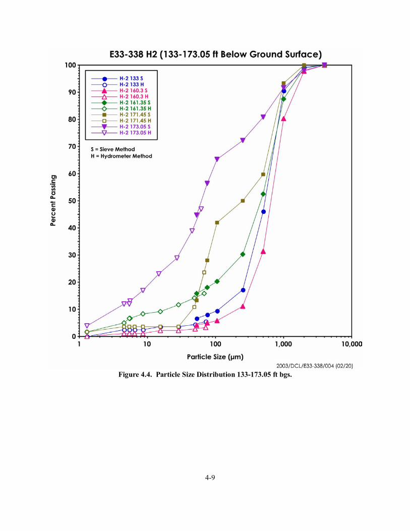
4-9

Figure 4.4. Particle Size Distribution 133-173.05 ft bgs.

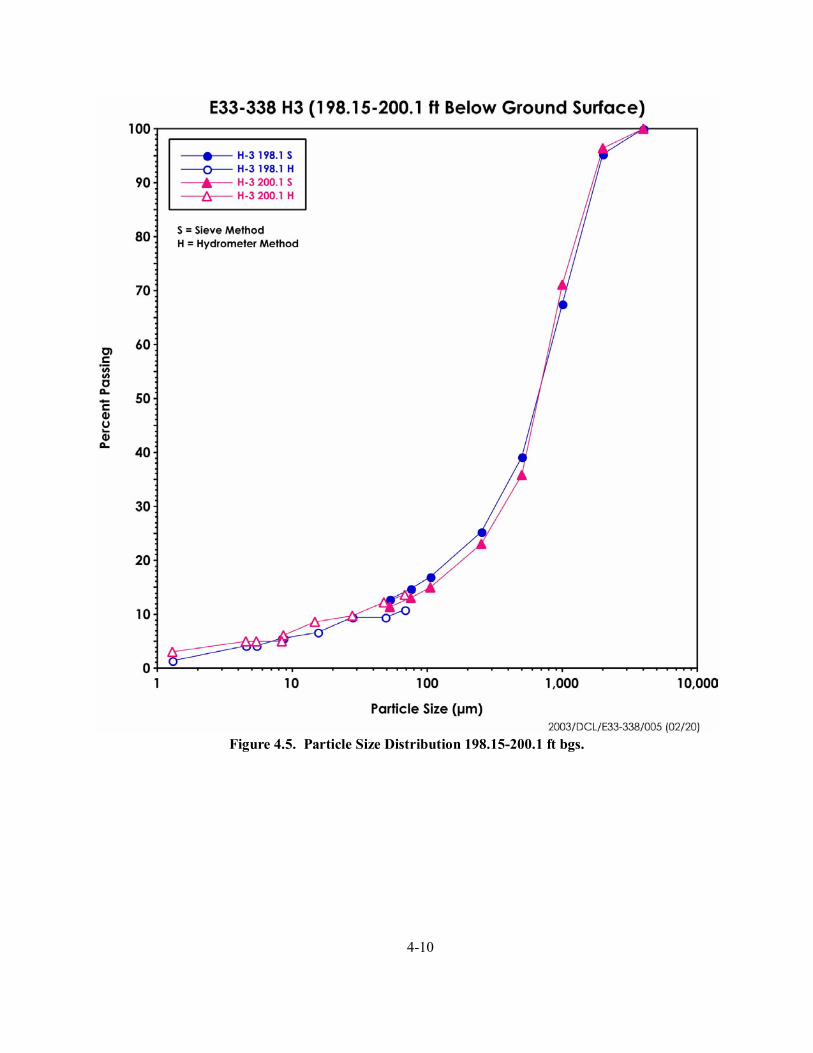
4-10

Figure 4.5. Particle Size Distribution 198.15-200.1 ft bgs.

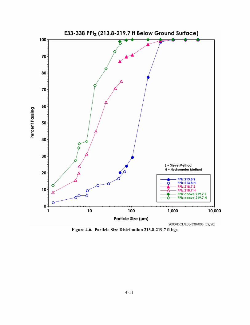
4-11

Figure 4.6. Particle Size Distribution 213.8-219.7 ft bgs.

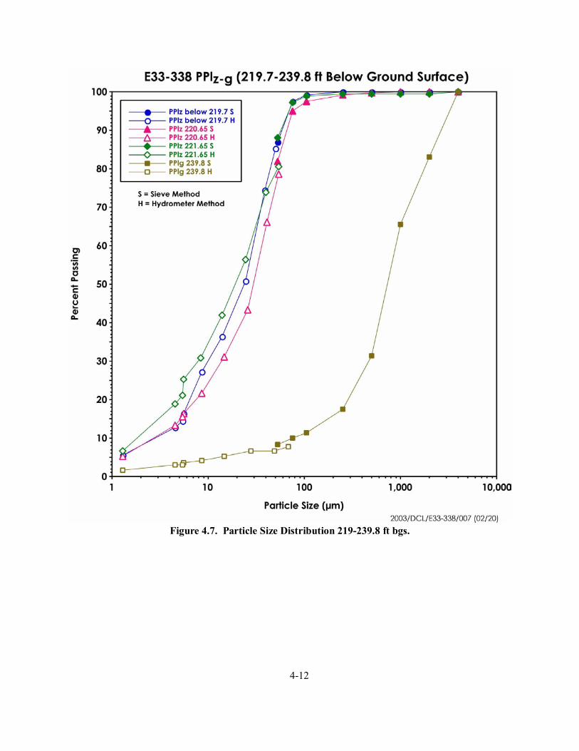
4-12

Figure 4.7. Particle Size Distribution 219-239.8 ft bgs.

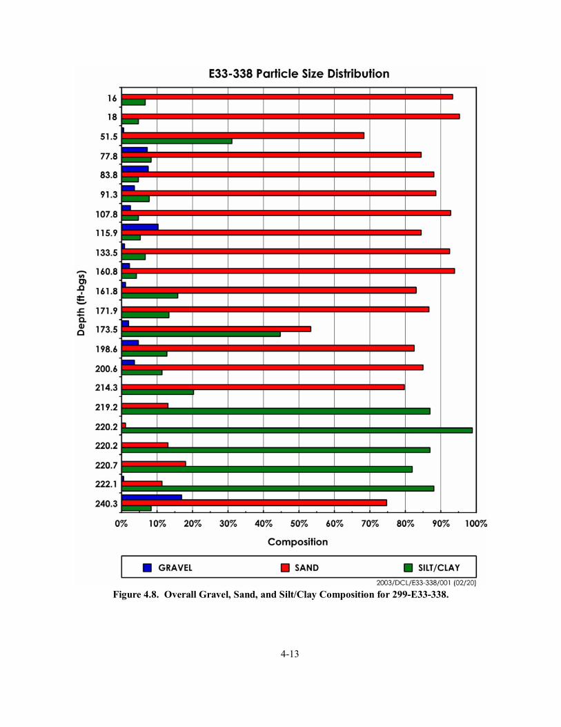
4-13

Figure 4.8. Overall Gravel, Sand, and Silt/Clay Composition for 299-E33-338.

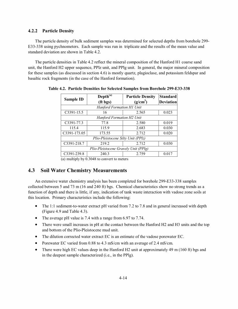
4-14

4.2.2 Particle Density

The particle density of bulk sediment samples was determined for selected depths from borehole 299-E33-338 using pychnometers. Each sample was run in triplicate and the results of the mean value and standard deviation are shown in Table 4.2.

The particle densities in Table 4.2 reflect the mineral composition of the Hanford H1 coarse sand unit, the Hanford H2 upper sequence, PPlz unit, and PPlg unit. In general, the major mineral composition for these samples (as discussed in section 4.6) is mostly quartz, plagioclase, and potassium feldspar and basaltic rock fragments (in the case of the Hanford formation).

Table 4.2. Particle Densities for Selected Samples from Borehole 299-E33-338

Sample ID Depth(a) (ft bgs)

Particle Density (g/cm3)

Standard Deviation

Hanford Formation H1 Unit C3391-15.5 16 2.565 0.023

Hanford Formation H2 Unit C3391-77.3 77.8 2.580 0.019

115.4 115.9 2.683 0.030 C3391-173.05 173.55 2.712 0.020

Plio-Pleistocene Silty Unit (PPlz) C3391-218.7 219.2 2.712 0.030

Plio-Pleistocene Gravely Unit (PPlg) C3391-239.8 240.3 2.759 0.017

(a) multiply by 0.3048 to convert to meters 4.3 Soil Water Chemistry Measurements

An extensive water chemistry analysis has been completed for borehole 299-E33-338 samples collected between 5 and 73 m (16 and 240 ft) bgs. Chemical characteristics show no strong trends as a function of depth and there is little, if any, indication of tank waste interaction with vadose zone soils at this location. Primary characteristics include the following:

• The 1:1 sediment-to-water extract pH varied from 7.2 to 7.8 and in general increased with depth (Figure 4.9 and Table 4.3).

• The average pH value is 7.4 with a range from 6.97 to 7.74. • There were small increases in pH at the contact between the Hanford H2 and H3 units and the top

and bottom of the Plio-Pleistocene mud unit. • The dilution corrected water extract EC is an estimate of the vadose porewater EC. • Porewater EC varied from 0.88 to 4.3 mS/cm with an average of 2.4 mS/cm. • There were high EC values deep in the Hanford H2 unit at approximately 49 m (160 ft) bgs and

in the deepest sample characterized (i.e., in the PPlg).

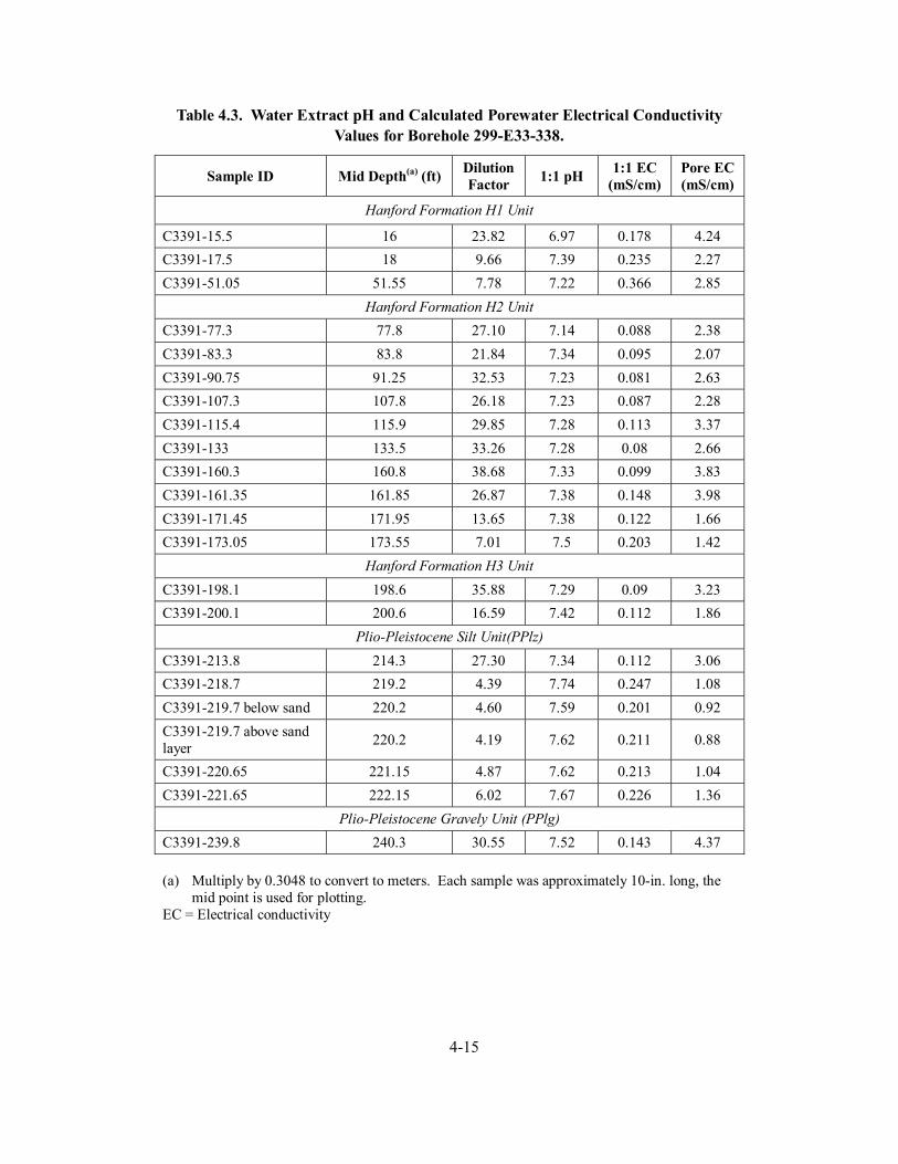
4-15

Table 4.3. Water Extract pH and Calculated Porewater Electrical Conductivity Values for Borehole 299-E33-338.

Sample ID Mid Depth(a) (ft) Dilution Factor 1:1 pH 1:1 EC

(mS/cm) Pore EC (mS/cm)

Hanford Formation H1 Unit

C3391-15.5 16 23.82 6.97 0.178 4.24 C3391-17.5 18 9.66 7.39 0.235 2.27 C3391-51.05 51.55 7.78 7.22 0.366 2.85

Hanford Formation H2 Unit C3391-77.3 77.8 27.10 7.14 0.088 2.38 C3391-83.3 83.8 21.84 7.34 0.095 2.07 C3391-90.75 91.25 32.53 7.23 0.081 2.63 C3391-107.3 107.8 26.18 7.23 0.087 2.28 C3391-115.4 115.9 29.85 7.28 0.113 3.37 C3391-133 133.5 33.26 7.28 0.08 2.66 C3391-160.3 160.8 38.68 7.33 0.099 3.83 C3391-161.35 161.85 26.87 7.38 0.148 3.98 C3391-171.45 171.95 13.65 7.38 0.122 1.66 C3391-173.05 173.55 7.01 7.5 0.203 1.42

Hanford Formation H3 Unit C3391-198.1 198.6 35.88 7.29 0.09 3.23 C3391-200.1 200.6 16.59 7.42 0.112 1.86

Plio-Pleistocene Silt Unit(PPlz) C3391-213.8 214.3 27.30 7.34 0.112 3.06 C3391-218.7 219.2 4.39 7.74 0.247 1.08 C3391-219.7 below sand 220.2 4.60 7.59 0.201 0.92 C3391-219.7 above sand layer 220.2 4.19 7.62 0.211 0.88

C3391-220.65 221.15 4.87 7.62 0.213 1.04 C3391-221.65 222.15 6.02 7.67 0.226 1.36

Plio-Pleistocene Gravely Unit (PPlg) C3391-239.8 240.3 30.55 7.52 0.143 4.37

(a) Multiply by 0.3048 to convert to meters. Each sample was approximately 10-in. long, the mid point is used for plotting.

EC = Electrical conductivity

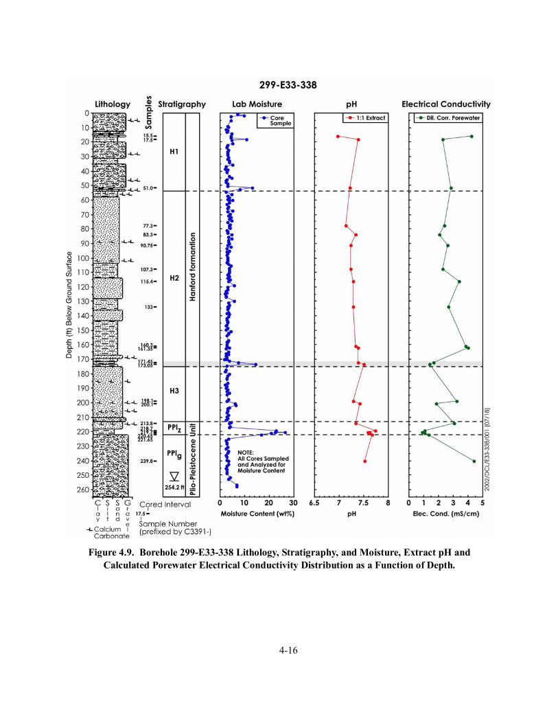
4-16

Figure 4.9. Borehole 299-E33-338 Lithology, Stratigraphy, and Moisture, Extract pH and

Calculated Porewater Electrical Conductivity Distribution as a Function of Depth.

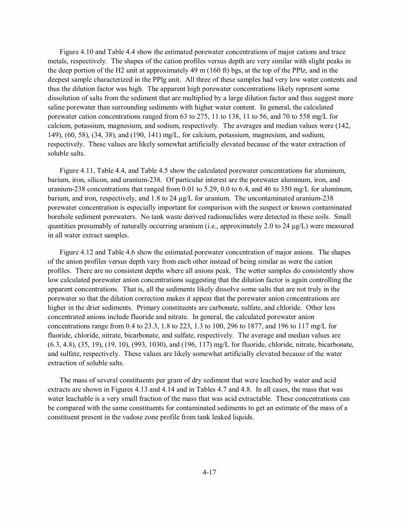
4-17

Figure 4.10 and Table 4.4 show the estimated porewater concentrations of major cations and trace metals, respectively. The shapes of the cation profiles versus depth are very similar with slight peaks in the deep portion of the H2 unit at approximately 49 m (160 ft) bgs, at the top of the PPlz, and in the deepest sample characterized in the PPlg unit. All three of these samples had very low water contents and thus the dilution factor was high. The apparent high porewater concentrations likely represent some dissolution of salts from the sediment that are multiplied by a large dilution factor and thus suggest more saline porewater than surrounding sediments with higher water content. In general, the calculated porewater cation concentrations ranged from 63 to 275, 11 to 138, 11 to 56, and 70 to 558 mg/L for calcium, potassium, magnesium, and sodium, respectively. The averages and median values were (142, 149), (60, 58), (34, 38), and (190, 141) mg/L, for calcium, potassium, magnesium, and sodium, respectively. These values are likely somewhat artificially elevated because of the water extraction of soluble salts.

Figure 4.11, Table 4.4, and Table 4.5 show the calculated porewater concentrations for aluminum, barium, iron, silicon, and uranium-238. Of particular interest are the porewater aluminum, iron, and uranium-238 concentrations that ranged from 0.01 to 5.29, 0.0 to 6.4, and 46 to 350 mg/L for aluminum, barium, and iron, respectively, and 1.8 to 24 µg/L for uranium. The uncontaminated uranium-238 porewater concentration is especially important for comparison with the suspect or known contaminated borehole sediment porewaters. No tank waste derived radionuclides were detected in these soils. Small quantities presumably of naturally occurring uranium (i.e., approximately 2.0 to 24 µg/L) were measured in all water extract samples.

Figure 4.12 and Table 4.6 show the estimated porewater concentration of major anions. The shapes of the anion profiles versus depth vary from each other instead of being similar as were the cation profiles. There are no consistent depths where all anions peak. The wetter samples do consistently show low calculated porewater anion concentrations suggesting that the dilution factor is again controlling the apparent concentrations. That is, all the sediments likely dissolve some salts that are not truly in the porewater so that the dilution correction makes it appear that the porewater anion concentrations are higher in the drier sediments. Primary constituents are carbonate, sulfate, and chloride. Other less concentrated anions include fluoride and nitrate. In general, the calculated porewater anion concentrations range from 0.4 to 23.3, 1.8 to 223, 1.3 to 100, 296 to 1877, and 196 to 117 mg/L for fluoride, chloride, nitrate, bicarbonate, and sulfate, respectively. The average and median values are (6.3, 4.8), (35, 19), (19, 10), (993, 1030), and (196, 117) mg/L for fluoride, chloride, nitrate, bicarbonate, and sulfate, respectively. These values are likely somewhat artificially elevated because of the water extraction of soluble salts.

The mass of several constituents per gram of dry sediment that were leached by water and acid extracts are shown in Figures 4.13 and 4.14 and in Tables 4.7 and 4.8. In all cases, the mass that was water leachable is a very small fraction of the mass that was acid extractable. These concentrations can be compared with the same constituents for contaminated sediments to get an estimate of the mass of a constituent present in the vadose zone profile from tank leaked liquids.

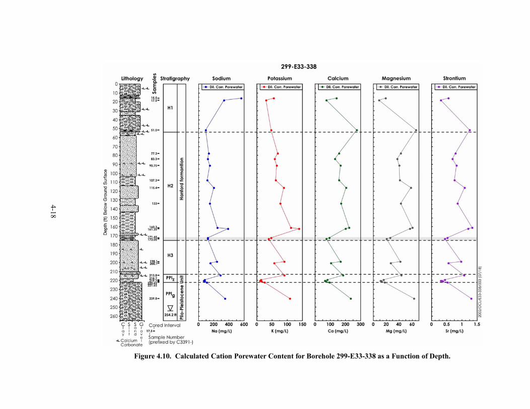
4-18

Figure 4.10. Calculated Cation Porewater Content for Borehole 299-E33-338 as a Function of Depth.

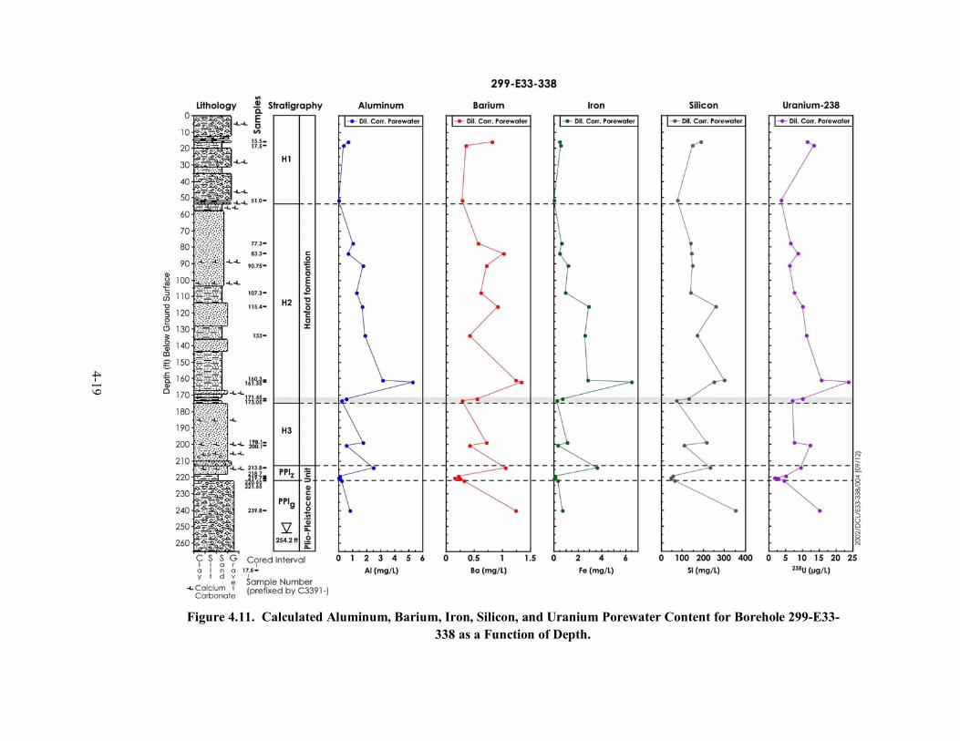
4-19

Figure 4.11. Calculated Aluminum, Barium, Iron, Silicon, and Uranium Porewater Content for Borehole 299-E33-338 as a Function of Depth.

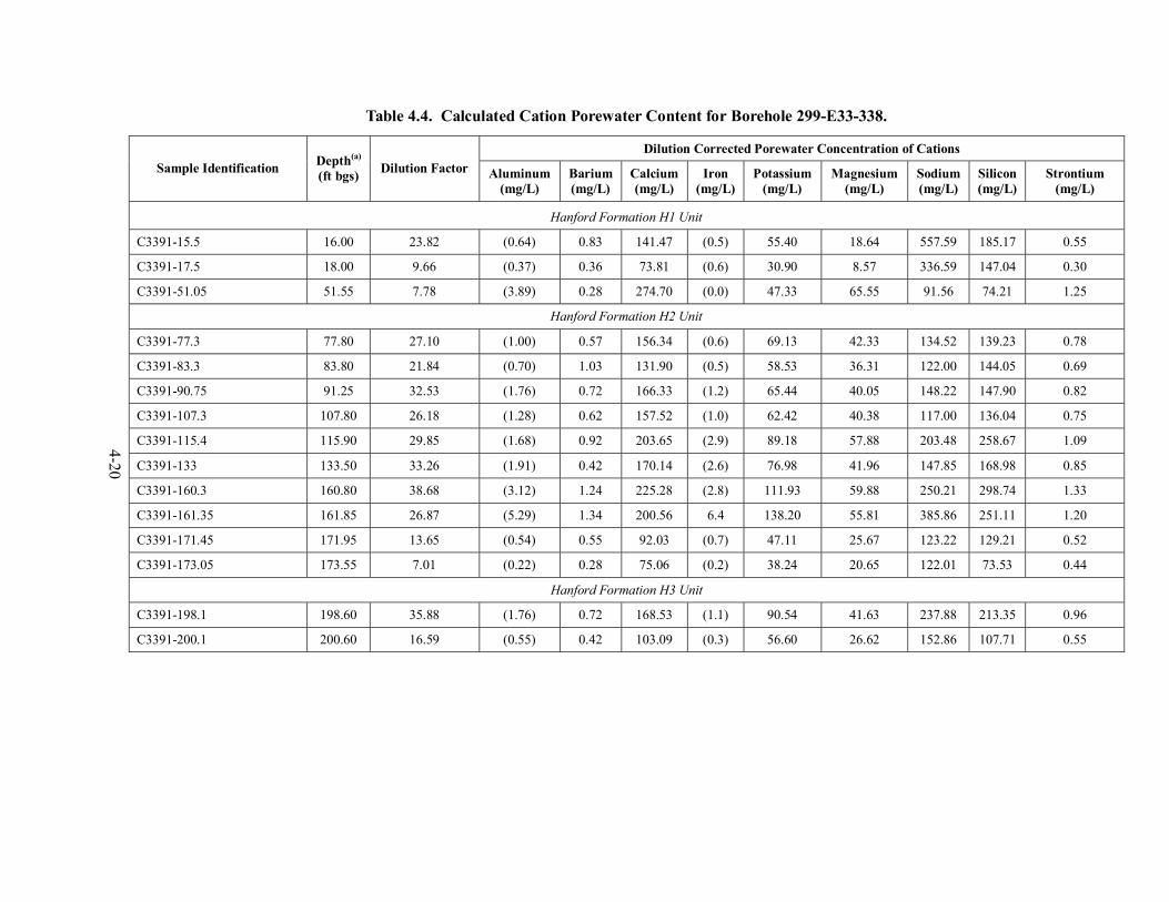
4-20

Table 4.4. Calculated Cation Porewater Content for Borehole 299-E33-338.

Dilution Corrected Porewater Concentration of Cations Sample Identification Depth(a)

(ft bgs) Dilution Factor Aluminum(mg/L)

Barium(mg/L)

Calcium (mg/L)

Iron (mg/L)

Potassium(mg/L)

Magnesium(mg/L)

Sodium(mg/L)

Silicon(mg/L)

Strontium (mg/L)

Hanford Formation H1 Unit

C3391-15.5 16.00 23.82 (0.64) 0.83 141.47 (0.5) 55.40 18.64 557.59 185.17 0.55

C3391-17.5 18.00 9.66 (0.37) 0.36 73.81 (0.6) 30.90 8.57 336.59 147.04 0.30

C3391-51.05 51.55 7.78 (3.89) 0.28 274.70 (0.0) 47.33 65.55 91.56 74.21 1.25

Hanford Formation H2 Unit

C3391-77.3 77.80 27.10 (1.00) 0.57 156.34 (0.6) 69.13 42.33 134.52 139.23 0.78

C3391-83.3 83.80 21.84 (0.70) 1.03 131.90 (0.5) 58.53 36.31 122.00 144.05 0.69

C3391-90.75 91.25 32.53 (1.76) 0.72 166.33 (1.2) 65.44 40.05 148.22 147.90 0.82

C3391-107.3 107.80 26.18 (1.28) 0.62 157.52 (1.0) 62.42 40.38 117.00 136.04 0.75

C3391-115.4 115.90 29.85 (1.68) 0.92 203.65 (2.9) 89.18 57.88 203.48 258.67 1.09

C3391-133 133.50 33.26 (1.91) 0.42 170.14 (2.6) 76.98 41.96 147.85 168.98 0.85

C3391-160.3 160.80 38.68 (3.12) 1.24 225.28 (2.8) 111.93 59.88 250.21 298.74 1.33

C3391-161.35 161.85 26.87 (5.29) 1.34 200.56 6.4 138.20 55.81 385.86 251.11 1.20

C3391-171.45 171.95 13.65 (0.54) 0.55 92.03 (0.7) 47.11 25.67 123.22 129.21 0.52

C3391-173.05 173.55 7.01 (0.22) 0.28 75.06 (0.2) 38.24 20.65 122.01 73.53 0.44

Hanford Formation H3 Unit

C3391-198.1 198.60 35.88 (1.76) 0.72 168.53 (1.1) 90.54 41.63 237.88 213.35 0.96

C3391-200.1 200.60 16.59 (0.55) 0.42 103.09 (0.3) 56.60 26.62 152.86 107.71 0.55

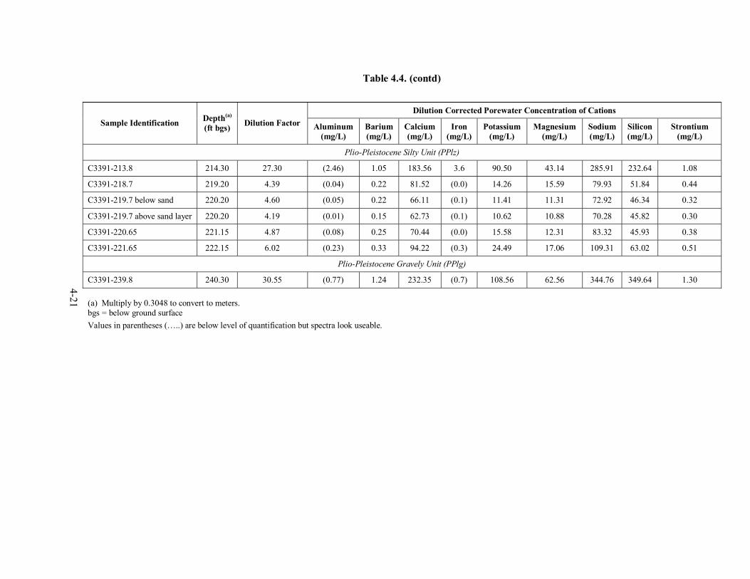
4-21

Table 4.4. (contd)

Dilution Corrected Porewater Concentration of Cations Sample Identification Depth(a)

(ft bgs) Dilution Factor Aluminum(mg/L)

Barium(mg/L)

Calcium (mg/L)

Iron (mg/L)

Potassium(mg/L)

Magnesium(mg/L)

Sodium(mg/L)

Silicon(mg/L)

Strontium (mg/L)

Plio-Pleistocene Silty Unit (PPlz)

C3391-213.8 214.30 27.30 (2.46) 1.05 183.56 3.6 90.50 43.14 285.91 232.64 1.08

C3391-218.7 219.20 4.39 (0.04) 0.22 81.52 (0.0) 14.26 15.59 79.93 51.84 0.44

C3391-219.7 below sand 220.20 4.60 (0.05) 0.22 66.11 (0.1) 11.41 11.31 72.92 46.34 0.32

C3391-219.7 above sand layer 220.20 4.19 (0.01) 0.15 62.73 (0.1) 10.62 10.88 70.28 45.82 0.30

C3391-220.65 221.15 4.87 (0.08) 0.25 70.44 (0.0) 15.58 12.31 83.32 45.93 0.38

C3391-221.65 222.15 6.02 (0.23) 0.33 94.22 (0.3) 24.49 17.06 109.31 63.02 0.51

Plio-Pleistocene Gravely Unit (PPlg)

C3391-239.8 240.30 30.55 (0.77) 1.24 232.35 (0.7) 108.56 62.56 344.76 349.64 1.30

(a) Multiply by 0.3048 to convert to meters. bgs = below ground surface Values in parentheses (…..) are below level of quantification but spectra look useable.

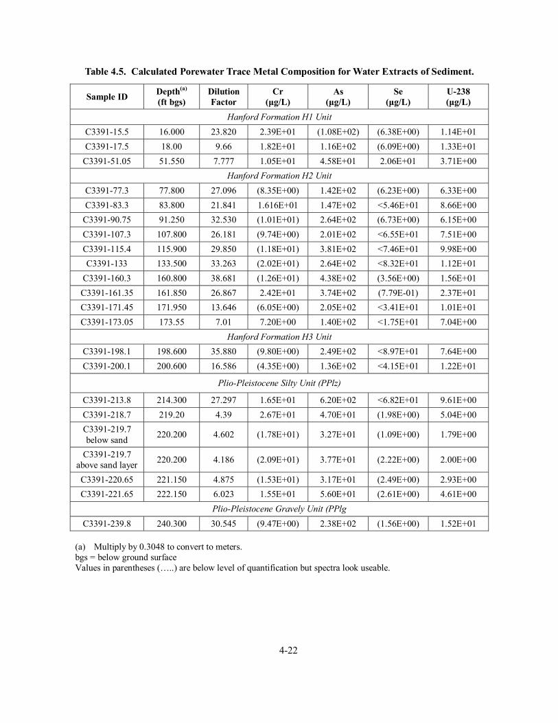
4-22

Table 4.5. Calculated Porewater Trace Metal Composition for Water Extracts of Sediment.

Sample ID Depth(a) (ft bgs)

Dilution Factor

Cr (µg/L)

As (µg/L)

Se (µg/L)

U-238 (µg/L)

Hanford Formation H1 Unit C3391-15.5 16.000 23.820 2.39E+01 (1.08E+02) (6.38E+00) 1.14E+01 C3391-17.5 18.00 9.66 1.82E+01 1.16E+02 (6.09E+00) 1.33E+01

C3391-51.05 51.550 7.777 1.05E+01 4.58E+01 2.06E+01 3.71E+00 Hanford Formation H2 Unit

C3391-77.3 77.800 27.096 (8.35E+00) 1.42E+02 (6.23E+00) 6.33E+00 C3391-83.3 83.800 21.841 1.616E+01 1.47E+02 <5.46E+01 8.66E+00

C3391-90.75 91.250 32.530 (1.01E+01) 2.64E+02 (6.73E+00) 6.15E+00 C3391-107.3 107.800 26.181 (9.74E+00) 2.01E+02 <6.55E+01 7.51E+00 C3391-115.4 115.900 29.850 (1.18E+01) 3.81E+02 <7.46E+01 9.98E+00 C3391-133 133.500 33.263 (2.02E+01) 2.64E+02 <8.32E+01 1.12E+01

C3391-160.3 160.800 38.681 (1.26E+01) 4.38E+02 (3.56E+00) 1.56E+01 C3391-161.35 161.850 26.867 2.42E+01 3.74E+02 (7.79E-01) 2.37E+01 C3391-171.45 171.950 13.646 (6.05E+00) 2.05E+02 <3.41E+01 1.01E+01 C3391-173.05 173.55 7.01 7.20E+00 1.40E+02 <1.75E+01 7.04E+00

Hanford Formation H3 Unit C3391-198.1 198.600 35.880 (9.80E+00) 2.49E+02 <8.97E+01 7.64E+00 C3391-200.1 200.600 16.586 (4.35E+00) 1.36E+02 <4.15E+01 1.22E+01

Plio-Pleistocene Silty Unit (PPlz)

C3391-213.8 214.300 27.297 1.65E+01 6.20E+02 <6.82E+01 9.61E+00 C3391-218.7 219.20 4.39 2.67E+01 4.70E+01 (1.98E+00) 5.04E+00 C3391-219.7 below sand 220.200 4.602 (1.78E+01) 3.27E+01 (1.09E+00) 1.79E+00

C3391-219.7 above sand layer 220.200 4.186 (2.09E+01) 3.77E+01 (2.22E+00) 2.00E+00

C3391-220.65 221.150 4.875 (1.53E+01) 3.17E+01 (2.49E+00) 2.93E+00 C3391-221.65 222.150 6.023 1.55E+01 5.60E+01 (2.61E+00) 4.61E+00

Plio-Pleistocene Gravely Unit (PPlg C3391-239.8 240.300 30.545 (9.47E+00) 2.38E+02 (1.56E+00) 1.52E+01

(a) Multiply by 0.3048 to convert to meters. bgs = below ground surface Values in parentheses (…..) are below level of quantification but spectra look useable.

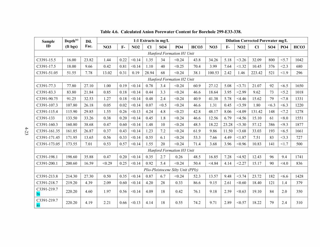
4-23

Table 4.6. Calculated Anion Porewater Content for Borehole 299-E33-338.

1:1 Extracts in mg/L Dilution Corrected Porewater mg/L Sample ID

Depth(a)

(ft bgs) Dil. Fac. NO3 F- NO2 Cl SO4 PO4 HCO3 NO3 F- NO2 Cl SO4 PO4 HCO3

Hanford Formation H1 Unit C3391-15.5 16.00 23.82 1.44 0.22 <0.14 1.35 34 <0.24 43.8 34.26 5.18 <3.26 32.09 800 <5.7 1042 C3391-17.5 18.00 9.66 0.42 0.81 <0.14 1.10 40 <0.25 70.4 3.99 7.64 <1.32 10.45 376 <2.3 680 C3391-51.05 51.55 7.78 13.02 0.31 0.19 28.94 68 <0.24 38.1 100.53 2.42 1.46 223.42 521 <1.9 296

Hanford Formation H2 Unit C3391-77.3 77.80 27.10 1.00 0.19 <0.14 0.78 3.4 <0.24 60.9 27.12 5.08 <3.71 21.07 92 <6.5 1650 C3391-83.3 83.80 21.84 0.85 0.18 <0.14 0.44 3.3 <0.24 46.6 18.64 3.95 <2.99 9.62 73 <5.2 1018 C3391-90.75 91.25 32.53 1.27 0.18 <0.14 0.48 2.4 <0.24 40.9 41.38 5.78 <4.46 15.62 79 <7.8 1331 C3391-107.3 107.80 26.18 0.05 0.02 <0.14 0.07 <0.5 <0.24 46.6 1.31 0.45 <3.59 1.80 <6.3 <6.3 1220 C3391-115.4 115.90 29.85 1.55 0.26 <0.13 4.24 4.8 <0.23 42.8 48.17 8.06 <4.09 131.42 148 <7.2 1278 C3391-133 133.50 33.26 0.38 0.20 <0.14 0.45 1.8 <0.24 46.6 12.56 6.79 <4.56 15.10 61 <8.0 1551 C3391-160.3 160.80 38.68 0.47 0.60 <0.14 1.48 10 <0.24 48.5 18.22 23.28 <5.30 57.12 386 <9.3 1877 C3391-161.35 161.85 26.87 0.37 0.43 <0.14 1.23 7.2 <0.24 61.9 9.86 11.50 <3.68 33.03 193 <6.5 1661 C3391-171.45 171.95 13.65 0.56 0.33 <0.14 0.55 6.1 <0.24 53.3 7.66 4.49 <1.87 7.51 83 <3.3 727 C3391-173.05 173.55 7.01 0.53 0.57 <0.14 1.55 20 <0.24 71.4 3.68 3.96 <0.96 10.83 141 <1.7 500

Hanford Formation H3 Unit C3391-198.1 198.60 35.88 0.47 0.20 <0.14 0.35 2.7 0.26 48.5 16.85 7.28 <4.92 12.43 96 9.4 1741 C3391-200.1 200.60 16.59 <0.29 0.25 <0.14 0.92 5.4 <0.24 50.4 <4.84 4.14 <2.27 15.17 90 <4.0 836

Plio-Pleistocene Silty Unit (PPlz) C3391-213.8 214.30 27.30 0.50 0.35 <0.14 0.87 6.7 <0.24 52.3 13.57 9.48 <3.74 23.72 182 <6.6 1428 C3391-218.7 219.20 4.39 2.09 0.60 <0.14 4.20 28 0.33 86.6 9.15 2.61 <0.60 18.40 121 1.4 379 C3391-219.7 bs 220.20 4.60 1.97 0.56 <0.14 4.09 18 0.42 76.1 9.18 2.59 <0.63 19.10 84 2.0 350

C3391-219.7 as 220.20 4.19 2.21 0.66 <0.13 4.14 18 0.55 74.2 9.71 2.89 <0.57 18.22 79 2.4 310

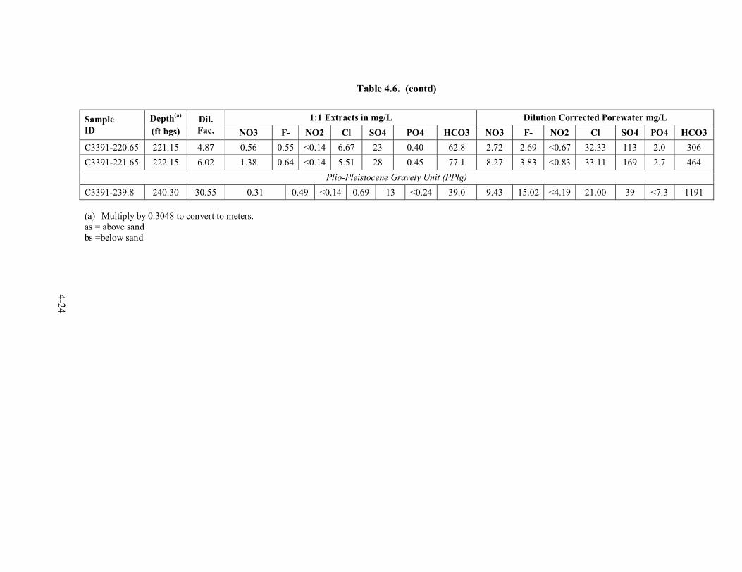
4-24

Table 4.6. (contd)

1:1 Extracts in mg/L Dilution Corrected Porewater mg/L Sample ID

Depth(a)

(ft bgs) Dil. Fac. NO3 F- NO2 Cl SO4 PO4 HCO3 NO3 F- NO2 Cl SO4 PO4 HCO3

C3391-220.65 221.15 4.87 0.56 0.55 <0.14 6.67 23 0.40 62.8 2.72 2.69 <0.67 32.33 113 2.0 306 C3391-221.65 222.15 6.02 1.38 0.64 <0.14 5.51 28 0.45 77.1 8.27 3.83 <0.83 33.11 169 2.7 464

Plio-Pleistocene Gravely Unit (PPlg) C3391-239.8 240.30 30.55 0.31 0.49 <0.14 0.69 13 <0.24 39.0 9.43 15.02 <4.19 21.00 39 <7.3 1191

(a) Multiply by 0.3048 to convert to meters. as = above sand bs =below sand

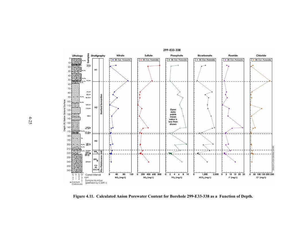
4-25

Figure 4.11. Calculated Anion Porewater Content for Borehole 299-E33-338 as a Function of Depth.

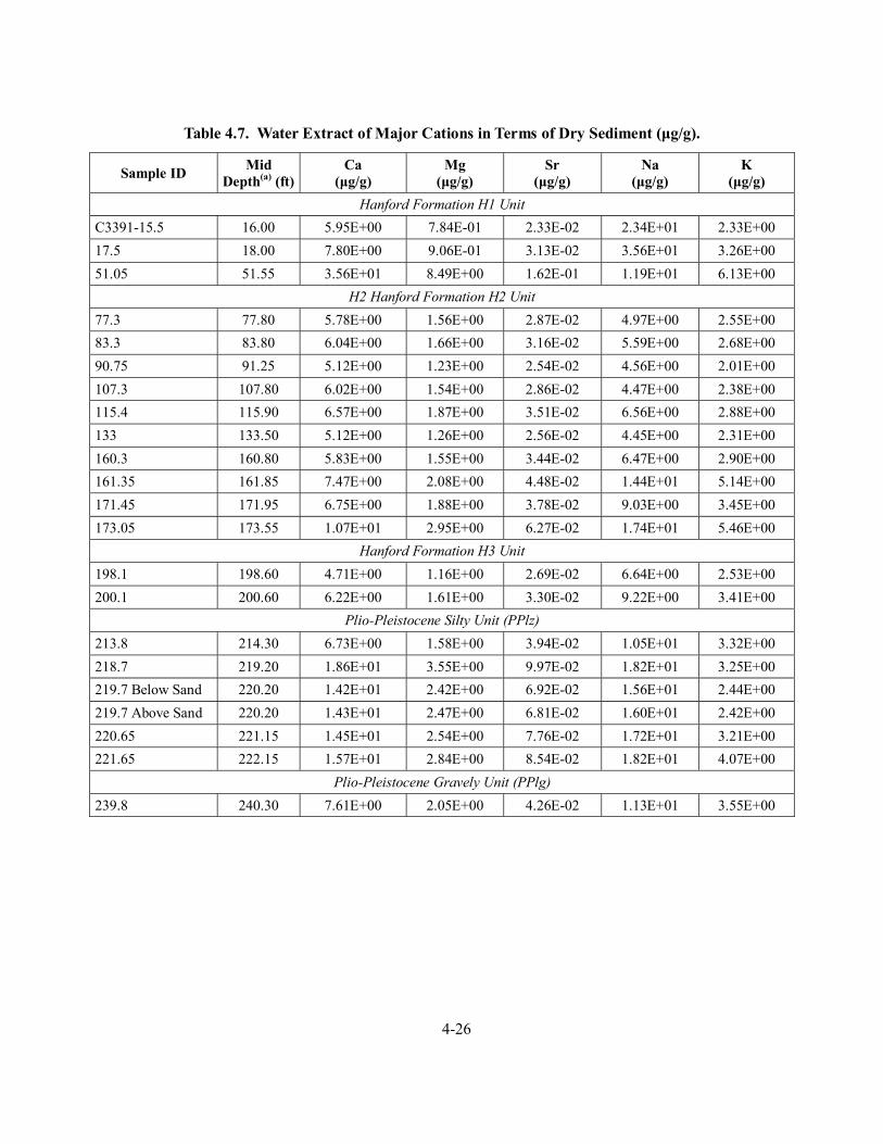
4-26

Table 4.7. Water Extract of Major Cations in Terms of Dry Sediment (µg/g).

Sample ID Mid Depth(a) (ft)

Ca (µg/g)

Mg (µg/g)

Sr (µg/g)

Na (µg/g)

K (µg/g)

Hanford Formation H1 Unit C3391-15.5 16.00 5.95E+00 7.84E-01 2.33E-02 2.34E+01 2.33E+00 17.5 18.00 7.80E+00 9.06E-01 3.13E-02 3.56E+01 3.26E+00 51.05 51.55 3.56E+01 8.49E+00 1.62E-01 1.19E+01 6.13E+00

H2 Hanford Formation H2 Unit 77.3 77.80 5.78E+00 1.56E+00 2.87E-02 4.97E+00 2.55E+00 83.3 83.80 6.04E+00 1.66E+00 3.16E-02 5.59E+00 2.68E+00 90.75 91.25 5.12E+00 1.23E+00 2.54E-02 4.56E+00 2.01E+00 107.3 107.80 6.02E+00 1.54E+00 2.86E-02 4.47E+00 2.38E+00 115.4 115.90 6.57E+00 1.87E+00 3.51E-02 6.56E+00 2.88E+00 133 133.50 5.12E+00 1.26E+00 2.56E-02 4.45E+00 2.31E+00 160.3 160.80 5.83E+00 1.55E+00 3.44E-02 6.47E+00 2.90E+00 161.35 161.85 7.47E+00 2.08E+00 4.48E-02 1.44E+01 5.14E+00 171.45 171.95 6.75E+00 1.88E+00 3.78E-02 9.03E+00 3.45E+00 173.05 173.55 1.07E+01 2.95E+00 6.27E-02 1.74E+01 5.46E+00

Hanford Formation H3 Unit 198.1 198.60 4.71E+00 1.16E+00 2.69E-02 6.64E+00 2.53E+00 200.1 200.60 6.22E+00 1.61E+00 3.30E-02 9.22E+00 3.41E+00

Plio-Pleistocene Silty Unit (PPlz) 213.8 214.30 6.73E+00 1.58E+00 3.94E-02 1.05E+01 3.32E+00 218.7 219.20 1.86E+01 3.55E+00 9.97E-02 1.82E+01 3.25E+00 219.7 Below Sand 220.20 1.42E+01 2.42E+00 6.92E-02 1.56E+01 2.44E+00 219.7 Above Sand 220.20 1.43E+01 2.47E+00 6.81E-02 1.60E+01 2.42E+00 220.65 221.15 1.45E+01 2.54E+00 7.76E-02 1.72E+01 3.21E+00 221.65 222.15 1.57E+01 2.84E+00 8.54E-02 1.82E+01 4.07E+00

Plio-Pleistocene Gravely Unit (PPlg) 239.8 240.30 7.61E+00 2.05E+00 4.26E-02 1.13E+01 3.55E+00

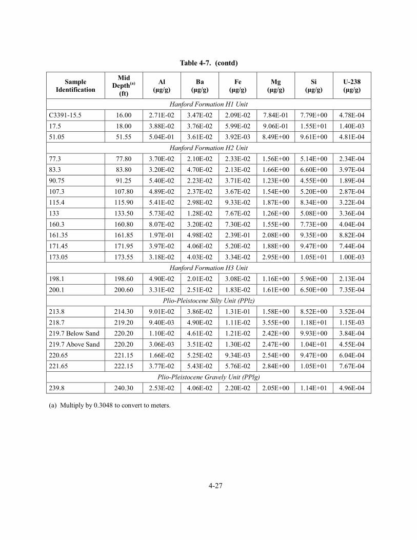
4-27

Table 4-7. (contd)

Sample Identification

Mid Depth(a)

(ft)

Al (µg/g)

Ba (µg/g)

Fe (µg/g)

Mg (µg/g)

Si (µg/g)

U-238 (µg/g)

Hanford Formation H1 Unit C3391-15.5 16.00 2.71E-02 3.47E-02 2.09E-02 7.84E-01 7.79E+00 4.78E-04 17.5 18.00 3.88E-02 3.76E-02 5.99E-02 9.06E-01 1.55E+01 1.40E-03 51.05 51.55 5.04E-01 3.61E-02 3.92E-03 8.49E+00 9.61E+00 4.81E-04

Hanford Formation H2 Unit 77.3 77.80 3.70E-02 2.10E-02 2.33E-02 1.56E+00 5.14E+00 2.34E-04 83.3 83.80 3.20E-02 4.70E-02 2.13E-02 1.66E+00 6.60E+00 3.97E-04 90.75 91.25 5.40E-02 2.23E-02 3.71E-02 1.23E+00 4.55E+00 1.89E-04 107.3 107.80 4.89E-02 2.37E-02 3.67E-02 1.54E+00 5.20E+00 2.87E-04 115.4 115.90 5.41E-02 2.98E-02 9.33E-02 1.87E+00 8.34E+00 3.22E-04 133 133.50 5.73E-02 1.28E-02 7.67E-02 1.26E+00 5.08E+00 3.36E-04 160.3 160.80 8.07E-02 3.20E-02 7.30E-02 1.55E+00 7.73E+00 4.04E-04 161.35 161.85 1.97E-01 4.98E-02 2.39E-01 2.08E+00 9.35E+00 8.82E-04 171.45 171.95 3.97E-02 4.06E-02 5.20E-02 1.88E+00 9.47E+00 7.44E-04 173.05 173.55 3.18E-02 4.03E-02 3.34E-02 2.95E+00 1.05E+01 1.00E-03

Hanford Formation H3 Unit 198.1 198.60 4.90E-02 2.01E-02 3.08E-02 1.16E+00 5.96E+00 2.13E-04 200.1 200.60 3.31E-02 2.51E-02 1.83E-02 1.61E+00 6.50E+00 7.35E-04

Plio-Pleistocene Silty Unit (PPlz) 213.8 214.30 9.01E-02 3.86E-02 1.31E-01 1.58E+00 8.52E+00 3.52E-04 218.7 219.20 9.40E-03 4.90E-02 1.11E-02 3.55E+00 1.18E+01 1.15E-03 219.7 Below Sand 220.20 1.10E-02 4.61E-02 1.21E-02 2.42E+00 9.93E+00 3.84E-04 219.7 Above Sand 220.20 3.06E-03 3.51E-02 1.30E-02 2.47E+00 1.04E+01 4.55E-04 220.65 221.15 1.66E-02 5.25E-02 9.34E-03 2.54E+00 9.47E+00 6.04E-04 221.65 222.15 3.77E-02 5.43E-02 5.76E-02 2.84E+00 1.05E+01 7.67E-04

Plio-Pleistocene Gravely Unit (PPlg) 239.8 240.30 2.53E-02 4.06E-02 2.20E-02 2.05E+00 1.14E+01 4.96E-04

(a) Multiply by 0.3048 to convert to meters.

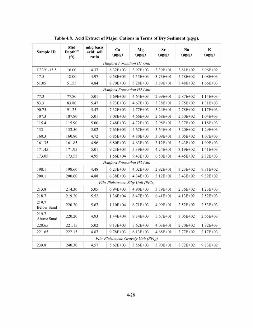
4-28

Table 4.8. Acid Extract of Major Cations in Terms of Dry Sediment (µg/g).

Sample ID Mid

Depth(a) (ft)

ml/g basisacid: soil

ratio

Ca (µg/g)

Mg (µg/g)

Sr (µg/g)

Na (µg/g)

K (µg/g)

Hanford Formation H1 Unit C3391-15.5 16.00 4.37 8.32E+03 3.97E+03 3.39E+01 3.81E+02 8.96E+02 17.5 18.00 4.97 9.58E+03 4.55E+03 3.73E+01 5.58E+02 1.08E+03 51.05 51.55 4.84 8.70E+03 5.28E+03 3.89E+01 3.48E+02 1.66E+03

Hanford Formation H2 Unit 77.3 77.80 5.01 7.69E+03 4.64E+03 2.99E+01 2.87E+02 1.14E+03 83.3 83.80 5.47 8.23E+03 4.67E+03 3.38E+01 2.75E+02 1.31E+03 90.75 91.25 5.47 7.32E+03 4.77E+03 3.24E+01 2.78E+02 1.17E+03 107.3 107.80 5.01 7.08E+03 4.66E+03 2.68E+01 2.50E+02 1.04E+03 115.4 115.90 5.00 7.48E+03 4.72E+03 2.98E+01 3.37E+02 1.18E+03 133 133.50 5.02 7.65E+03 4.67E+03 3.64E+01 3.20E+02 1.29E+03 160.3 160.80 4.72 6.85E+03 4.80E+03 3.09E+01 3.05E+02 1.07E+03 161.35 161.85 4.96 6.80E+03 4.63E+03 3.12E+01 3.43E+02 1.09E+03 171.45 171.95 5.01 9.23E+03 5.39E+03 4.24E+01 3.19E+02 1.41E+03 173.05 173.55 4.95 1.56E+04 9.43E+03 6.50E+01 4.45E+02 2.82E+03

Hanford Formation H3 Unit 198.1 198.60 4.48 6.23E+03 4.02E+03 2.92E+01 3.23E+02 9.31E+02 200.1 200.60 4.88 6.38E+03 4.34E+03 3.12E+01 3.43E+02 9.82E+02

Plio-Pleistocene Silty Unit (PPlz) 213.8 214.30 5.05 6.94E+03 4.90E+03 3.39E+01 2.76E+02 1.23E+03 218.7 219.20 5.52 1.36E+04 8.47E+03 6.41E+01 4.13E+02 2.52E+03 219.7 Below Sand 220.20 5.67 1.10E+04 6.71E+03 4.99E+01 3.52E+02 2.53E+03

219.7 Above Sand 220.20 4.93 1.44E+04 9.34E+03 5.67E+01 3.05E+02 2.65E+03

220.65 221.15 5.02 9.13E+03 5.62E+03 4.03E+01 2.70E+02 1.92E+03 221.65 222.15 4.87 9.78E+03 6.13E+03 4.68E+01 3.77E+02 2.17E+03

Plio-Pleistocene Gravely Unit (PPlg) 239.8 240.30 4.57 5.62E+03 3.56E+03 3.90E+01 3.72E+02 9.83E+02

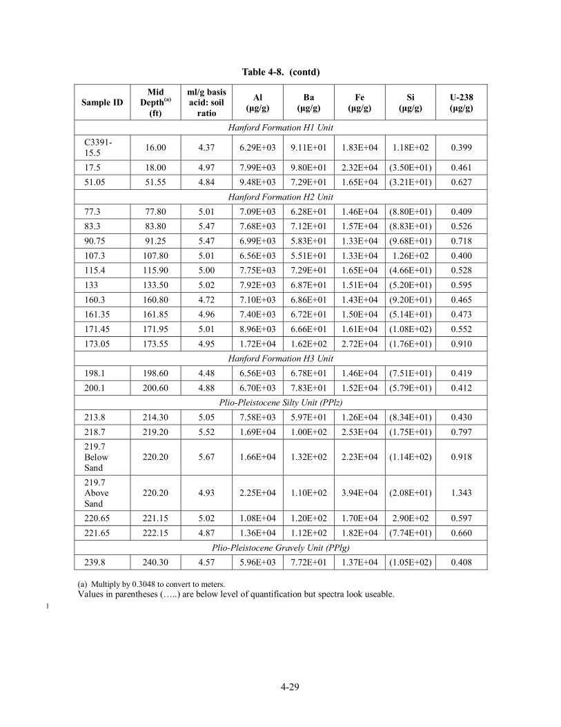
4-29

Table 4-8. (contd)

Sample ID Mid

Depth(a) (ft)

ml/g basisacid: soil

ratio

Al (µg/g)

Ba (µg/g)

Fe (µg/g)

Si (µg/g)

U-238 (µg/g)

Hanford Formation H1 Unit C3391-15.5 16.00 4.37 6.29E+03 9.11E+01 1.83E+04 1.18E+02 0.399

17.5 18.00 4.97 7.99E+03 9.80E+01 2.32E+04 (3.50E+01) 0.461 51.05 51.55 4.84 9.48E+03 7.29E+01 1.65E+04 (3.21E+01) 0.627

Hanford Formation H2 Unit 77.3 77.80 5.01 7.09E+03 6.28E+01 1.46E+04 (8.80E+01) 0.409 83.3 83.80 5.47 7.68E+03 7.12E+01 1.57E+04 (8.83E+01) 0.526 90.75 91.25 5.47 6.99E+03 5.83E+01 1.33E+04 (9.68E+01) 0.718 107.3 107.80 5.01 6.56E+03 5.51E+01 1.33E+04 1.26E+02 0.400 115.4 115.90 5.00 7.75E+03 7.29E+01 1.65E+04 (4.66E+01) 0.528 133 133.50 5.02 7.92E+03 6.87E+01 1.51E+04 (5.20E+01) 0.595 160.3 160.80 4.72 7.10E+03 6.86E+01 1.43E+04 (9.20E+01) 0.465 161.35 161.85 4.96 7.40E+03 6.72E+01 1.50E+04 (5.14E+01) 0.473 171.45 171.95 5.01 8.96E+03 6.66E+01 1.61E+04 (1.08E+02) 0.552 173.05 173.55 4.95 1.72E+04 1.62E+02 2.72E+04 (1.76E+01) 0.910

Hanford Formation H3 Unit 198.1 198.60 4.48 6.56E+03 6.78E+01 1.46E+04 (7.51E+01) 0.419 200.1 200.60 4.88 6.70E+03 7.83E+01 1.52E+04 (5.79E+01) 0.412

Plio-Pleistocene Silty Unit (PPlz) 213.8 214.30 5.05 7.58E+03 5.97E+01 1.26E+04 (8.34E+01) 0.430 218.7 219.20 5.52 1.69E+04 1.00E+02 2.53E+04 (1.75E+01) 0.797 219.7 Below Sand

220.20 5.67 1.66E+04 1.32E+02 2.23E+04 (1.14E+02) 0.918

219.7 Above Sand

220.20 4.93 2.25E+04 1.10E+02 3.94E+04 (2.08E+01) 1.343

220.65 221.15 5.02 1.08E+04 1.20E+02 1.70E+04 2.90E+02 0.597 221.65 222.15 4.87 1.36E+04 1.12E+02 1.82E+04 (7.74E+01) 0.660

Plio-Pleistocene Gravely Unit (PPlg) 239.8 240.30 4.57 5.96E+03 7.72E+01 1.37E+04 (1.05E+02) 0.408

(a) Multiply by 0.3048 to convert to meters. Values in parentheses (…..) are below level of quantification but spectra look useable.

1

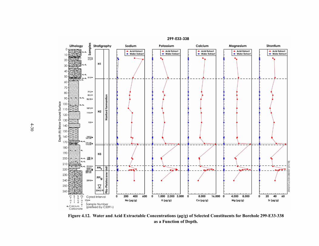
4-30

Figure 4.12. Water and Acid Extractable Concentrations (µg/g) of Selected Constituents for Borehole 299-E33-338 as a Function of Depth.

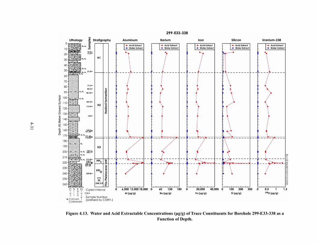
4-31

Figure 4.13. Water and Acid Extractable Concentrations (µg/g) of Trace Constituents for Borehole 299-E33-338 as a Function of Depth.

4-32

4.4 Soil Fusion Analysis

Table 4.9 shows the major and trace element constituents for each of the characterized sediments derived from using a lithium metaborate/tetraborate fusion method as described in Section 3.1.12. Very little difference is observed in the primary elemental oxide concentrations for any of the sediment samples as a function of depth or lithology. The primary elemental oxides reported are SiO2 (58.77-70.33 wt%), Al2O3 (12.7-15.73 wt%), Fe2O3 (3.74-7.92 wt%), CaO (3.02-4.80 wt%), Na2O (2.05-3.23 wt%), K2O (1.70-2.65 wt%), MgO (1.64-2.73 wt%), K2O (1.70-2.65 wt%), TiO2 (0.51-1.39 wt%), P2O5 (0.13-0.30 wt%), and MnO (0.07-0.12 wt%). An additional 35 trace elements are also reported in terms of ug/g of dry sediment with little if any significant variation in concentration.

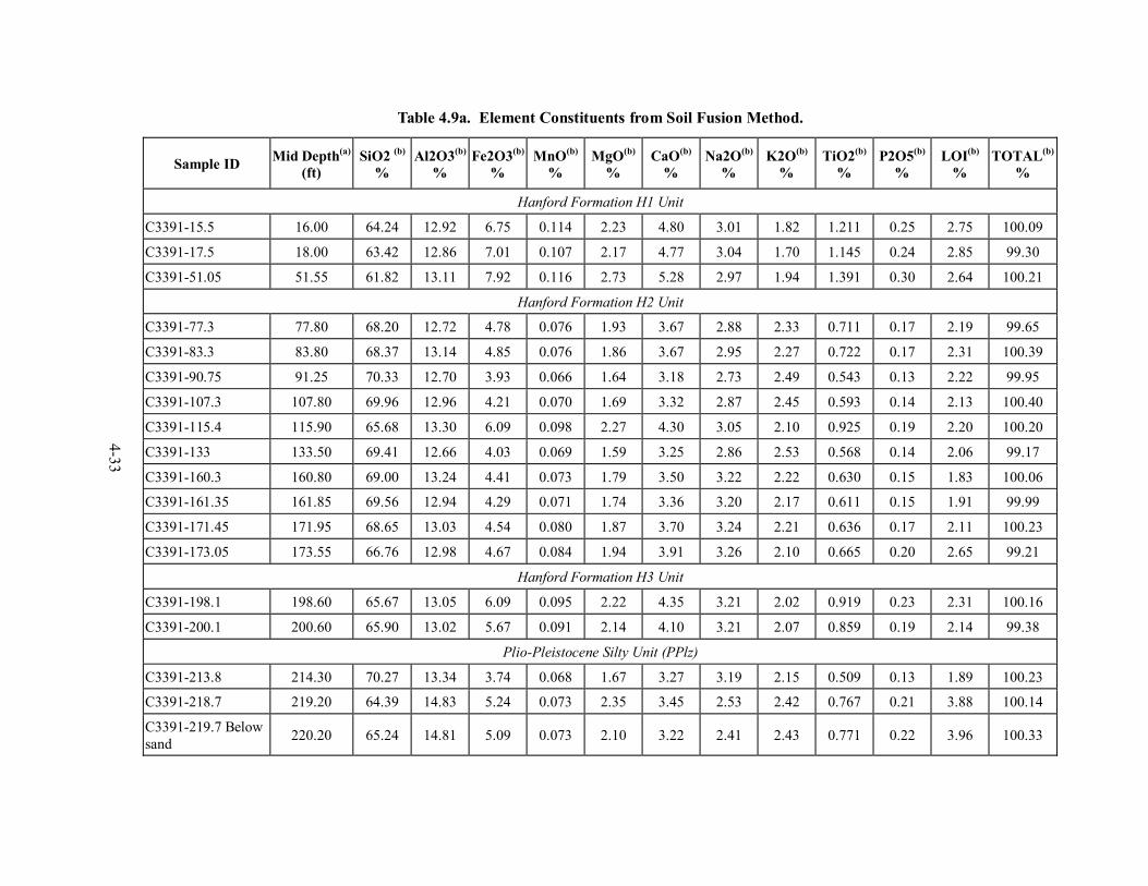
4-33

Table 4.9a. Element Constituents from Soil Fusion Method.

Sample ID Mid Depth(a) (ft)

SiO2 (b)

% Al2O3(b)

% Fe2O3(b)

% MnO(b)

% MgO(b)

% CaO(b)

% Na2O(b)

% K2O(b)

% TiO2(b)

% P2O5(b)

% LOI(b)

% TOTAL(b)

%

Hanford Formation H1 Unit

C3391-15.5 16.00 64.24 12.92 6.75 0.114 2.23 4.80 3.01 1.82 1.211 0.25 2.75 100.09

C3391-17.5 18.00 63.42 12.86 7.01 0.107 2.17 4.77 3.04 1.70 1.145 0.24 2.85 99.30

C3391-51.05 51.55 61.82 13.11 7.92 0.116 2.73 5.28 2.97 1.94 1.391 0.30 2.64 100.21

Hanford Formation H2 Unit

C3391-77.3 77.80 68.20 12.72 4.78 0.076 1.93 3.67 2.88 2.33 0.711 0.17 2.19 99.65

C3391-83.3 83.80 68.37 13.14 4.85 0.076 1.86 3.67 2.95 2.27 0.722 0.17 2.31 100.39

C3391-90.75 91.25 70.33 12.70 3.93 0.066 1.64 3.18 2.73 2.49 0.543 0.13 2.22 99.95

C3391-107.3 107.80 69.96 12.96 4.21 0.070 1.69 3.32 2.87 2.45 0.593 0.14 2.13 100.40

C3391-115.4 115.90 65.68 13.30 6.09 0.098 2.27 4.30 3.05 2.10 0.925 0.19 2.20 100.20

C3391-133 133.50 69.41 12.66 4.03 0.069 1.59 3.25 2.86 2.53 0.568 0.14 2.06 99.17

C3391-160.3 160.80 69.00 13.24 4.41 0.073 1.79 3.50 3.22 2.22 0.630 0.15 1.83 100.06

C3391-161.35 161.85 69.56 12.94 4.29 0.071 1.74 3.36 3.20 2.17 0.611 0.15 1.91 99.99

C3391-171.45 171.95 68.65 13.03 4.54 0.080 1.87 3.70 3.24 2.21 0.636 0.17 2.11 100.23

C3391-173.05 173.55 66.76 12.98 4.67 0.084 1.94 3.91 3.26 2.10 0.665 0.20 2.65 99.21

Hanford Formation H3 Unit

C3391-198.1 198.60 65.67 13.05 6.09 0.095 2.22 4.35 3.21 2.02 0.919 0.23 2.31 100.16

C3391-200.1 200.60 65.90 13.02 5.67 0.091 2.14 4.10 3.21 2.07 0.859 0.19 2.14 99.38

Plio-Pleistocene Silty Unit (PPlz)

C3391-213.8 214.30 70.27 13.34 3.74 0.068 1.67 3.27 3.19 2.15 0.509 0.13 1.89 100.23

C3391-218.7 219.20 64.39 14.83 5.24 0.073 2.35 3.45 2.53 2.42 0.767 0.21 3.88 100.14

C3391-219.7 Below sand 220.20 65.24 14.81 5.09 0.073 2.10 3.22 2.41 2.43 0.771 0.22 3.96 100.33

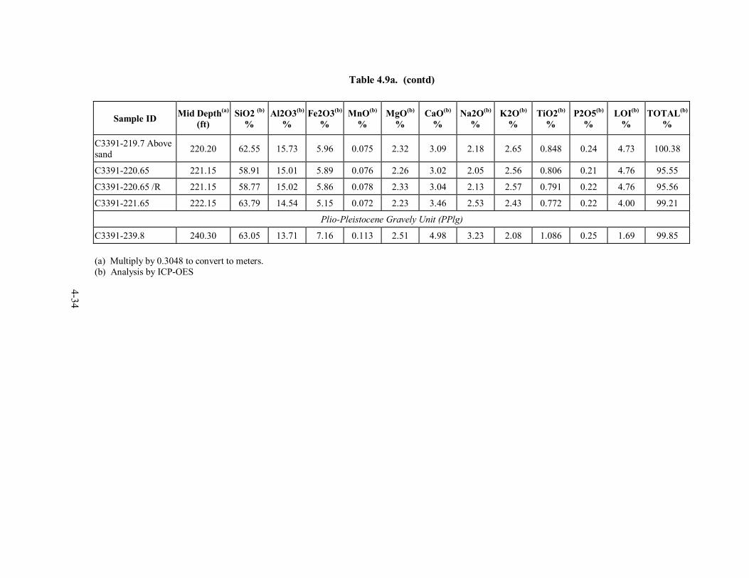
4-34

Table 4.9a. (contd)

Sample ID Mid Depth(a) (ft)

SiO2 (b)

% Al2O3(b)

% Fe2O3(b)

% MnO(b)

% MgO(b)

% CaO(b)

% Na2O(b)

% K2O(b)

% TiO2(b)

% P2O5(b)

% LOI(b)

% TOTAL(b)

%

C3391-219.7 Above sand 220.20 62.55 15.73 5.96 0.075 2.32 3.09 2.18 2.65 0.848 0.24 4.73 100.38

C3391-220.65 221.15 58.91 15.01 5.89 0.076 2.26 3.02 2.05 2.56 0.806 0.21 4.76 95.55

C3391-220.65 /R 221.15 58.77 15.02 5.86 0.078 2.33 3.04 2.13 2.57 0.791 0.22 4.76 95.56

C3391-221.65 222.15 63.79 14.54 5.15 0.072 2.23 3.46 2.53 2.43 0.772 0.22 4.00 99.21

Plio-Pleistocene Gravely Unit (PPlg)

C3391-239.8 240.30 63.05 13.71 7.16 0.113 2.51 4.98 3.23 2.08 1.086 0.25 1.69 99.85

(a) Multiply by 0.3048 to convert to meters. (b) Analysis by ICP-OES

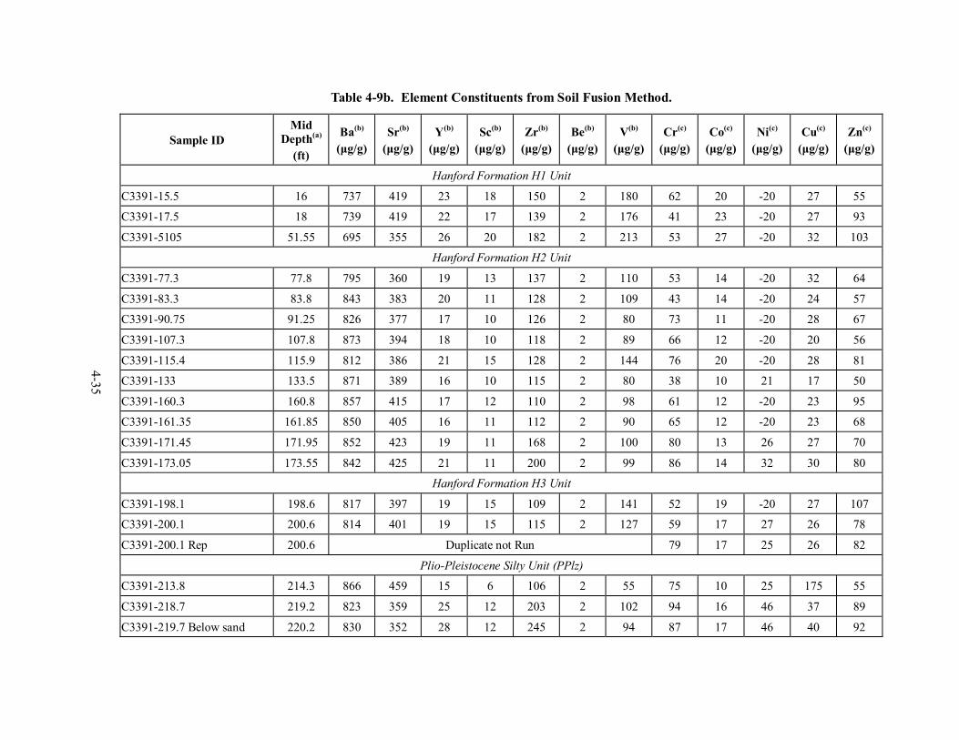
4-35

Table 4-9b. Element Constituents from Soil Fusion Method.

Sample ID Mid

Depth(a) (ft)

Ba(b) (µg/g)

Sr(b) (µg/g)

Y(b) (µg/g)

Sc(b) (µg/g)

Zr(b) (µg/g)

Be(b) (µg/g)

V(b) (µg/g)

Cr(c) (µg/g)

Co(c) (µg/g)

Ni(c) (µg/g)

Cu(c) (µg/g)

Zn(c) (µg/g)

Hanford Formation H1 Unit

C3391-15.5 16 737 419 23 18 150 2 180 62 20 -20 27 55

C3391-17.5 18 739 419 22 17 139 2 176 41 23 -20 27 93

C3391-5105 51.55 695 355 26 20 182 2 213 53 27 -20 32 103

Hanford Formation H2 Unit

C3391-77.3 77.8 795 360 19 13 137 2 110 53 14 -20 32 64

C3391-83.3 83.8 843 383 20 11 128 2 109 43 14 -20 24 57

C3391-90.75 91.25 826 377 17 10 126 2 80 73 11 -20 28 67

C3391-107.3 107.8 873 394 18 10 118 2 89 66 12 -20 20 56

C3391-115.4 115.9 812 386 21 15 128 2 144 76 20 -20 28 81

C3391-133 133.5 871 389 16 10 115 2 80 38 10 21 17 50

C3391-160.3 160.8 857 415 17 12 110 2 98 61 12 -20 23 95

C3391-161.35 161.85 850 405 16 11 112 2 90 65 12 -20 23 68

C3391-171.45 171.95 852 423 19 11 168 2 100 80 13 26 27 70

C3391-173.05 173.55 842 425 21 11 200 2 99 86 14 32 30 80

Hanford Formation H3 Unit

C3391-198.1 198.6 817 397 19 15 109 2 141 52 19 -20 27 107

C3391-200.1 200.6 814 401 19 15 115 2 127 59 17 27 26 78

C3391-200.1 Rep 200.6 Duplicate not Run 79 17 25 26 82

Plio-Pleistocene Silty Unit (PPlz)

C3391-213.8 214.3 866 459 15 6 106 2 55 75 10 25 175 55

C3391-218.7 219.2 823 359 25 12 203 2 102 94 16 46 37 89

C3391-219.7 Below sand 220.2 830 352 28 12 245 2 94 87 17 46 40 92

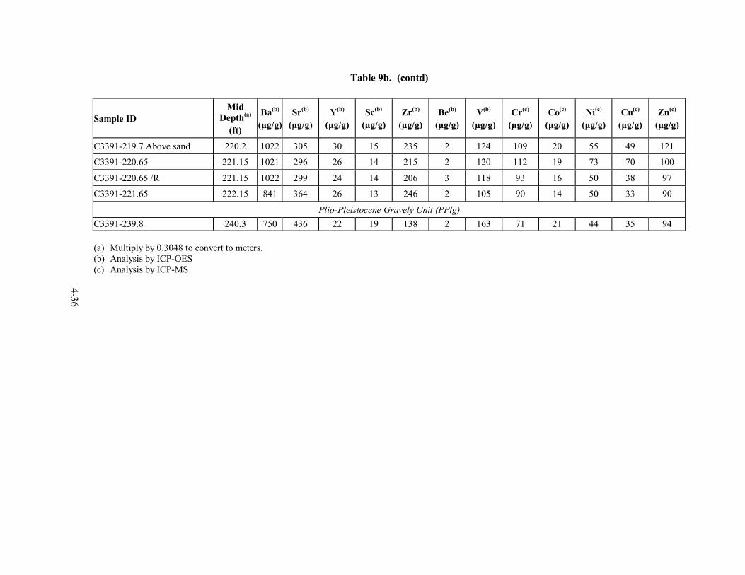
4-36

Table 9b. (contd)

Sample ID Mid

Depth(a) (ft)

Ba(b)

(µg/g)Sr(b)

(µg/g) Y(b)

(µg/g) Sc(b)

(µg/g) Zr(b)

(µg/g) Be(b)

(µg/g) V(b)

(µg/g) Cr(c)

(µg/g) Co(c)

(µg/g) Ni(c)

(µg/g) Cu(c)

(µg/g) Zn(c)

(µg/g)

C3391-219.7 Above sand 220.2 1022 305 30 15 235 2 124 109 20 55 49 121

C3391-220.65 221.15 1021 296 26 14 215 2 120 112 19 73 70 100

C3391-220.65 /R 221.15 1022 299 24 14 206 3 118 93 16 50 38 97

C3391-221.65 222.15 841 364 26 13 246 2 105 90 14 50 33 90

Plio-Pleistocene Gravely Unit (PPlg) C3391-239.8 240.3 750 436 22 19 138 2 163 71 21 44 35 94

(a) Multiply by 0.3048 to convert to meters. (b) Analysis by ICP-OES (c) Analysis by ICP-MS

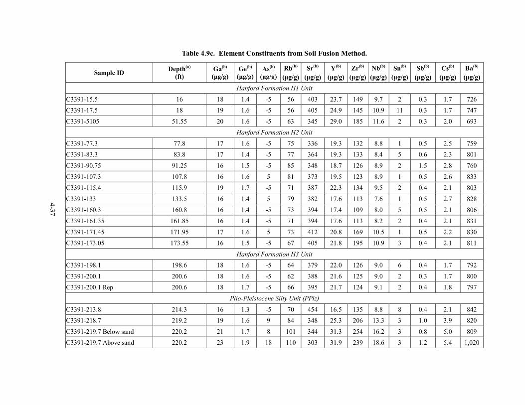
4-37

Table 4.9c. Element Constituents from Soil Fusion Method.

Sample ID Depth(a) (ft)

Ga(b)

(µg/g) Ge(b)

(µg/g)As(b)

(µg/g) Rb(b)

(µg/g)Sr(b)

(µg/g) Y(b)

(µg/g)Zr(b)

(µg/g)Nb(b)

(µg/g)Sn(b)

(µg/g)Sb(b)

(µg/g) Cs(b)

(µg/g) Ba(b)

(µg/g)

Hanford Formation H1 Unit

C3391-15.5 16 18 1.4 -5 56 403 23.7 149 9.7 2 0.3 1.7 726

C3391-17.5 18 19 1.6 -5 56 405 24.9 145 10.9 11 0.3 1.7 747

C3391-5105 51.55 20 1.6 -5 63 345 29.0 185 11.6 2 0.3 2.0 693

Hanford Formation H2 Unit

C3391-77.3 77.8 17 1.6 -5 75 336 19.3 132 8.8 1 0.5 2.5 759

C3391-83.3 83.8 17 1.4 -5 77 364 19.3 133 8.4 5 0.6 2.3 801

C3391-90.75 91.25 16 1.5 -5 85 348 18.7 126 8.9 2 1.5 2.8 760

C3391-107.3 107.8 16 1.6 5 81 373 19.5 123 8.9 1 0.5 2.6 833

C3391-115.4 115.9 19 1.7 -5 71 387 22.3 134 9.5 2 0.4 2.1 803

C3391-133 133.5 16 1.4 5 79 382 17.6 113 7.6 1 0.5 2.7 828

C3391-160.3 160.8 16 1.4 -5 73 394 17.4 109 8.0 5 0.5 2.1 806

C3391-161.35 161.85 16 1.4 -5 71 394 17.6 113 8.2 2 0.4 2.1 831

C3391-171.45 171.95 17 1.6 5 73 412 20.8 169 10.5 1 0.5 2.2 830

C3391-173.05 173.55 16 1.5 -5 67 405 21.8 195 10.9 3 0.4 2.1 811

Hanford Formation H3 Unit C3391-198.1 198.6 18 1.6 -5 64 379 22.0 126 9.0 6 0.4 1.7 792

C3391-200.1 200.6 18 1.6 -5 62 388 21.6 125 9.0 2 0.3 1.7 800

C3391-200.1 Rep 200.6 18 1.7 -5 66 395 21.7 124 9.1 2 0.4 1.8 797

Plio-Pleistocene Silty Unit (PPlz)

C3391-213.8 214.3 16 1.3 -5 70 454 16.5 135 8.8 8 0.4 2.1 842

C3391-218.7 219.2 19 1.6 9 84 348 25.3 206 13.3 3 1.0 3.9 820

C3391-219.7 Below sand 220.2 21 1.7 8 101 344 31.3 254 16.2 3 0.8 5.0 809

C3391-219.7 Above sand 220.2 23 1.9 18 110 303 31.9 239 18.6 3 1.2 5.4 1,020

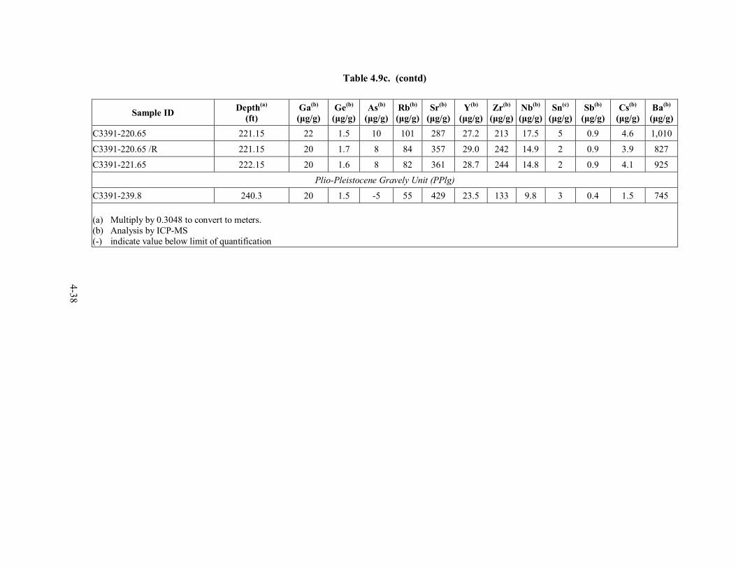
4-38

Table 4.9c. (contd)

Sample ID Depth(a) (ft)

Ga(b)

(µg/g) Ge(b)

(µg/g)As(b)

(µg/g) Rb(b)

(µg/g)Sr(b)

(µg/g) Y(b)

(µg/g)Zr(b)

(µg/g)Nb(b)

(µg/g)Sn(c)

(µg/g)Sb(b)

(µg/g) Cs(b)

(µg/g) Ba(b)

(µg/g)C3391-220.65 221.15 22 1.5 10 101 287 27.2 213 17.5 5 0.9 4.6 1,010

C3391-220.65 /R 221.15 20 1.7 8 84 357 29.0 242 14.9 2 0.9 3.9 827

C3391-221.65 222.15 20 1.6 8 82 361 28.7 244 14.8 2 0.9 4.1 925

Plio-Pleistocene Gravely Unit (PPlg)

C3391-239.8 240.3 20 1.5 -5 55 429 23.5 133 9.8 3 0.4 1.5 745

(a) Multiply by 0.3048 to convert to meters. (b) Analysis by ICP-MS (-) indicate value below limit of quantification

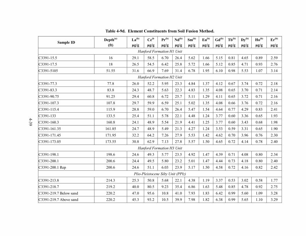
4-39

Table 4-9d. Element Constituents from Soil Fusion Method.

Sample ID Depth(a)

(ft) La(b) µg/g

Ce(b µg/g

Pr(b) µg/g

Nd(b) µg/g

Sm(b) µg/g

Eu(b) µg/g

Gd(b)

µg/g Tb(b) µg/g

Dy(b) µg/g

Ho(b) µg/g

Er(b) µg/g

Hanford Formation H1 Unit

C3391-15.5 16 29.1 58.5 6.70 26.4 5.62 1.66 5.15 0.81 4.65 0.89 2.59

C3391-17.5 18 26.5 54.5 6.42 25.8 5.72 1.66 5.12 0.85 4.71 0.93 2.76

C3391-5105 51.55 31.6 66.9 7.69 31.4 6.78 1.95 6.10 0.98 5.53 1.07 3.14

Hanford Formation H2 Unit

C3391-77.3 77.8 26.0 52.2 5.95 23.3 4.84 1.37 4.12 0.67 3.74 0.72 2.18

C3391-83.3 83.8 24.3 48.7 5.63 22.3 4.83 1.35 4.08 0.65 3.70 0.71 2.14

C3391-90.75 91.25 29.4 60.8 6.72 25.7 5.11 1.29 4.11 0.65 3.72 0.71 2.16

C3391-107.3 107.8 29.7 59.9 6.59 25.1 5.02 1.35 4.08 0.66 3.76 0.72 2.16

C3391-115.4 115.9 28.8 59.0 6.70 26.4 5.47 1.54 4.64 0.77 4.29 0.83 2.41

C3391-133 133.5 25.4 51.1 5.78 22.1 4.48 1.24 3.77 0.60 3.36 0.65 1.93

C3391-160.3 160.8 24.1 48.9 5.54 21.9 4.41 1.25 3.77 0.60 3.43 0.68 1.98

C3391-161.35 161.85 24.7 48.9 5.49 21.3 4.27 1.24 3.53 0.59 3.31 0.65 1.90

C3391-171.45 171.95 32.2 64.2 7.26 27.9 5.53 1.42 4.62 0.70 3.96 0.76 2.30

C3391-173.05 173.55 30.8 62.9 7.13 27.8 5.57 1.50 4.65 0.72 4.14 0.78 2.40

Hanford Formation H3 Unit

C3391-198.1 198.6 24.6 49.3 5.77 23.5 4.92 1.47 4.39 0.71 4.08 0.80 2.34

C3391-200.1 200.6 24.4 49.5 5.80 23.2 5.01 1.47 4.44 0.73 4.18 0.80 2.40

C3391-200.1 Rep 200.6 24.6 51.1 6.03 23.9 5.17 1.50 4.58 0.72 4.16 0.82 2.42

Plio-Pleistocene Silty Unit (PPlz)

C3391-213.8 214.3 25.3 50.8 5.68 22.1 4.38 1.19 3.37 0.53 3.02 0.58 1.77

C3391-218.7 219.2 40.0 80.5 9.23 35.4 6.86 1.63 5.48 0.85 4.78 0.92 2.75

C3391-219.7 Below sand 220.2 47.0 95.6 10.8 41.0 7.93 1.83 6.42 0.99 5.60 1.09 3.28

C3391-219.7 Above sand 220.2 45.3 93.2 10.5 39.9 7.98 1.82 6.38 0.99 5.65 1.10 3.29

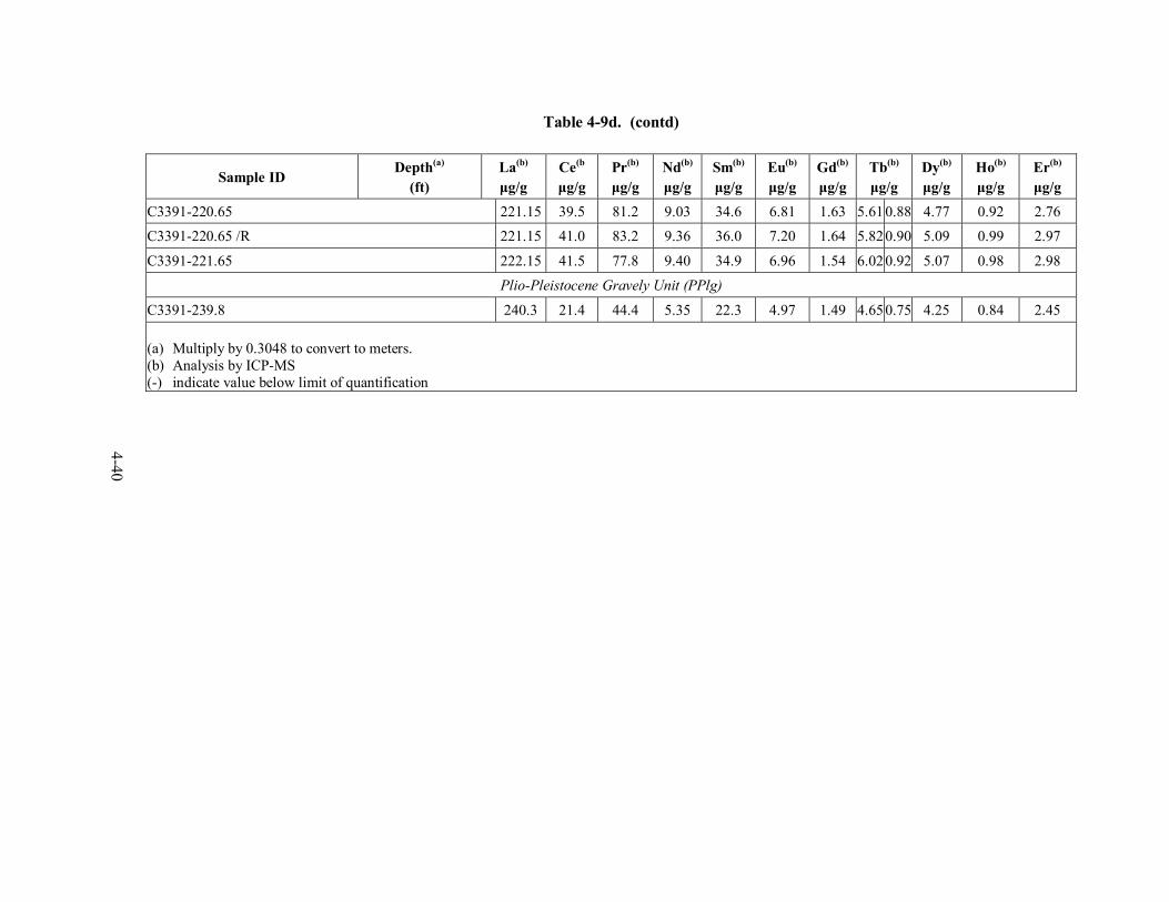
4-40

Table 4-9d. (contd)

Sample ID Depth(a)

(ft) La(b) µg/g

Ce(b µg/g

Pr(b) µg/g

Nd(b) µg/g

Sm(b) µg/g

Eu(b) µg/g

Gd(b)

µg/g Tb(b) µg/g

Dy(b) µg/g

Ho(b) µg/g

Er(b) µg/g

C3391-220.65 221.15 39.5 81.2 9.03 34.6 6.81 1.63 5.610.88 4.77 0.92 2.76

C3391-220.65 /R 221.15 41.0 83.2 9.36 36.0 7.20 1.64 5.820.90 5.09 0.99 2.97

C3391-221.65 222.15 41.5 77.8 9.40 34.9 6.96 1.54 6.020.92 5.07 0.98 2.98

Plio-Pleistocene Gravely Unit (PPlg)

C3391-239.8 240.3 21.4 44.4 5.35 22.3 4.97 1.49 4.650.75 4.25 0.84 2.45

(a) Multiply by 0.3048 to convert to meters. (b) Analysis by ICP-MS (-) indicate value below limit of quantification

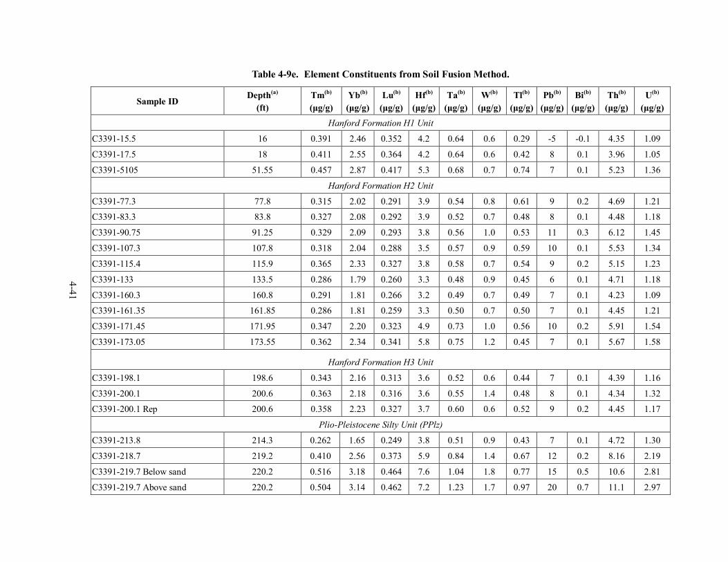
4-41

Table 4-9e. Element Constituents from Soil Fusion Method.

Sample ID Depth(a)

(ft) Tm(b) (µg/g)

Yb(b) (µg/g)

Lu(b) (µg/g)

Hf(b) (µg/g)

Ta(b) (µg/g)

W(b) (µg/g)

Tl(b) (µg/g)

Pb(b) (µg/g)

Bi(b) (µg/g)

Th(b) (µg/g)

U(b) (µg/g)

Hanford Formation H1 Unit

C3391-15.5 16 0.391 2.46 0.352 4.2 0.64 0.6 0.29 -5 -0.1 4.35 1.09

C3391-17.5 18 0.411 2.55 0.364 4.2 0.64 0.6 0.42 8 0.1 3.96 1.05

C3391-5105 51.55 0.457 2.87 0.417 5.3 0.68 0.7 0.74 7 0.1 5.23 1.36

Hanford Formation H2 Unit

C3391-77.3 77.8 0.315 2.02 0.291 3.9 0.54 0.8 0.61 9 0.2 4.69 1.21

C3391-83.3 83.8 0.327 2.08 0.292 3.9 0.52 0.7 0.48 8 0.1 4.48 1.18

C3391-90.75 91.25 0.329 2.09 0.293 3.8 0.56 1.0 0.53 11 0.3 6.12 1.45

C3391-107.3 107.8 0.318 2.04 0.288 3.5 0.57 0.9 0.59 10 0.1 5.53 1.34

C3391-115.4 115.9 0.365 2.33 0.327 3.8 0.58 0.7 0.54 9 0.2 5.15 1.23

C3391-133 133.5 0.286 1.79 0.260 3.3 0.48 0.9 0.45 6 0.1 4.71 1.18

C3391-160.3 160.8 0.291 1.81 0.266 3.2 0.49 0.7 0.49 7 0.1 4.23 1.09

C3391-161.35 161.85 0.286 1.81 0.259 3.3 0.50 0.7 0.50 7 0.1 4.45 1.21

C3391-171.45 171.95 0.347 2.20 0.323 4.9 0.73 1.0 0.56 10 0.2 5.91 1.54

C3391-173.05 173.55 0.362 2.34 0.341 5.8 0.75 1.2 0.45 7 0.1 5.67 1.58

Hanford Formation H3 Unit

C3391-198.1 198.6 0.343 2.16 0.313 3.6 0.52 0.6 0.44 7 0.1 4.39 1.16

C3391-200.1 200.6 0.363 2.18 0.316 3.6 0.55 1.4 0.48 8 0.1 4.34 1.32

C3391-200.1 Rep 200.6 0.358 2.23 0.327 3.7 0.60 0.6 0.52 9 0.2 4.45 1.17

Plio-Pleistocene Silty Unit (PPlz)

C3391-213.8 214.3 0.262 1.65 0.249 3.8 0.51 0.9 0.43 7 0.1 4.72 1.30

C3391-218.7 219.2 0.410 2.56 0.373 5.9 0.84 1.4 0.67 12 0.2 8.16 2.19

C3391-219.7 Below sand 220.2 0.516 3.18 0.464 7.6 1.04 1.8 0.77 15 0.5 10.6 2.81

C3391-219.7 Above sand 220.2 0.504 3.14 0.462 7.2 1.23 1.7 0.97 20 0.7 11.1 2.97

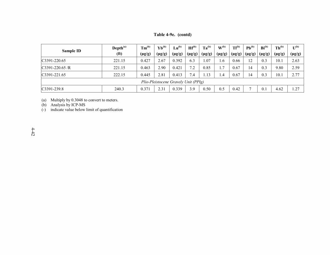
4-42

Table 4-9e. (contd)

Sample ID Depth(a)

(ft) Tm(b) (µg/g)

Yb(b) (µg/g)

Lu(b) (µg/g)

Hf(b) (µg/g)

Ta(b) (µg/g)

W(b) (µg/g)

Tl(b) (µg/g)

Pb(b) (µg/g)

Bi(b) (µg/g)

Th(b) (µg/g)

U(b) (µg/g)

C3391-220.65 221.15 0.427 2.67 0.392 6.3 1.07 1.6 0.66 12 0.3 10.1 2.63

C3391-220.65 /R 221.15 0.463 2.90 0.421 7.2 0.85 1.7 0.67 14 0.3 9.80 2.59

C3391-221.65 222.15 0.445 2.81 0.413 7.4 1.13 1.4 0.67 14 0.3 10.1 2.77

Plio-Pleistocene Gravely Unit (PPlg)

C3391-239.8 240.3 0.371 2.31 0.339 3.9 0.50 0.5 0.42 7 0.1 4.62 1.27

(a) Multiply by 0.3048 to convert to meters. (b) Analysis by ICP-MS (-) indicate value below limit of quantification

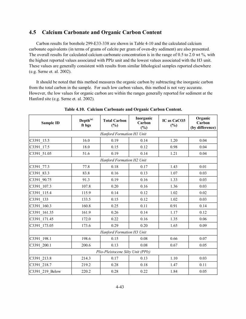
4-43

4.5 Calcium Carbonate and Organic Carbon Content

Carbon results for borehole 299-E33-338 are shown in Table 4-10 and the calculated calcium carbonate equivalents (in terms of grams of calcite per gram of oven-dry sediment) are also presented. The overall results for calculated calcium carbonate concentration is in the range of 0.5 to 2.0 wt %, with the highest reported values associated with PPlz unit and the lowest values associated with the H3 unit. These values are generally consistent with results from similar lithological samples reported elsewhere (e.g. Serne et. al. 2002).

It should be noted that this method measures the organic carbon by subtracting the inorganic carbon from the total carbon in the sample. For such low carbon values, this method is not very accurate. However, the low values for organic carbon are within the ranges generally reported for sediment at the Hanford site (e.g. Serne et. al. 2002).

Table 4.10. Calcium Carbonate and Organic Carbon Content.

Sample ID Depth(a) ft bgs

Total Carbon(%)

Inorganic Carbon

(%)

IC as CaCO3 (%)

Organic Carbon

(by difference)Hanford Formation H1 Unit

C3391_15.5 16.0 0.19 0.14 1.20 0.04 C3391_17.5 18.0 0.15 0.12 0.98 0.04 C3391_51.05 51.6 0.19 0.14 1.21 0.04

Hanford Formation H2 Unit C3391_77.3 77.8 0.18 0.17 1.43 0.01 C3391_83.3 83.8 0.16 0.13 1.07 0.03 C3391_90.75 91.3 0.19 0.16 1.33 0.03 C3391_107.3 107.8 0.20 0.16 1.36 0.03 C3391_115.4 115.9 0.14 0.12 1.02 0.02 C3391_133 133.5 0.15 0.12 1.02 0.03 C3391_160.3 160.8 0.25 0.11 0.91 0.14 C3391_161.35 161.9 0.26 0.14 1.17 0.12 C3391_171.45 172.0 0.22 0.16 1.35 0.06 C3391_173.05 173.6 0.29 0.20 1.65 0.09

Hanford Formation H3 Unit C3391_198.1 198.6 0.15 0.08 0.66 0.07 C3391_200.1 200.6 0.13 0.08 0.67 0.05

Plio-Pleistocene Silty Unit (PPlz) C3391_213.8 214.3 0.17 0.13 1.10 0.03 C3391_218.7 219.2 0.28 0.18 1.47 0.11 C3391_219_Below 220.2 0.28 0.22 1.84 0.05

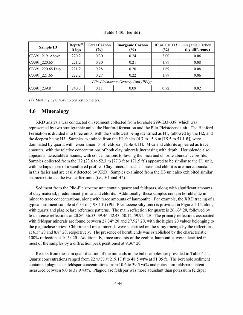
4-44

Table 4-10. (contd)

Sample ID Depth(a) ft bgs

Total Carbon(%)

Inorganic Carbon(%)

IC as CaCO3 (%)

Organic Carbon(by difference)

C3391_219_Above 220.2 0.30 0.24 2.00 0.06 C3391_220.65 221.2 0.30 0.21 1.79 0.08 C3391_220.65 Dup 221.2 0.28 0.20 1.69 0.08 C3391_221.65 222.2 0.27 0.22 1.79 0.06

Plio-Pleistocene Gravely Unit (PPlg) C3391_239.8 240.3 0.11 0.09 0.72 0.02

(a) Multiply by 0.3048 to convert to meters.

4.6 Mineralogy

XRD analysis was conducted on sediment collected from borehole 299-E33-338, which was represented by two stratigraphic units, the Hanford formation and the Plio-Pleistocene unit. The Hanford Formation is divided into three units, with the shallowest being identified as H1, followed by the H2, and the deepest being H3. Samples examined from the H1 facies (4.7 to 15.6 m [15.5 to 51.1 ft]) were dominated by quartz with lesser amounts of feldspar (Table 4.11). Mica and chlorite appeared as trace amounts, with the relative concentrations of both clay minerals increasing with depth. Hornblende also appears in detectable amounts, with concentrations following the mica and chlorite abundance profile. Samples collected from the H2 (23.6 to 52.3 m [77.3 ft to 171.5 ft]) appeared to be similar to the H1 unit, with perhaps more of a weathered profile. Clay minerals such as micas and chlorites are more abundant in this facies and are easily detected by XRD. Samples examined from the H3 unit also exhibited similar characteristics as the two earlier units (i.e., H1 and H2).

Sediment from the Plio-Pleistocene unit contain quartz and feldspars, along with significant amounts of clay material, predominantly mica and chlorite. Additionally, these samples contain hornblende in minor to trace concentrations, along with trace amounts of laumontite. For example, the XRD tracing of a typical sediment sample at 60.4 m (198.1 ft) (Plio-Pleistocene silty unit) is provided in Figure 4-15, along with quartz and plagioclase reference patterns. The main reflection for quartz is 26.63° 2θ, followed by less intense reflections at 20.86, 36.53, 39.46, 42.43, 50.12, 59.92° 2θ. The primary reflections associated with feldspar minerals are found between 27.34° 2θ and 27.92° 2θ, with the higher 2θ values belonging to the plagioclase series. Chlorite and mica minerals were identified on the x-ray tracings by the reflections at 6.3° 2θ and 8.8° 2θ, respectively. The presence of hornblende was established by the characteristic 100% reflection at 10.5° 2θ. Additionally, trace amounts of the zeolite, laumontite, were identified in most of the samples by a diffraction peak positioned at 9.36° 2θ.

Results from the semi quantification of the minerals in the bulk samples are provided in Table 4.11. Quartz concentrations ranged from 22 wt% at 219.17 ft to 48.5 wt% at 51.05 ft. The borehole sediment contained plagioclase feldspar concentrations from 10.6 to 39.5 wt% and potassium feldspar content measured between 9.0 to 37.9 wt%. Plagioclase feldspar was more abundant than potassium feldspar

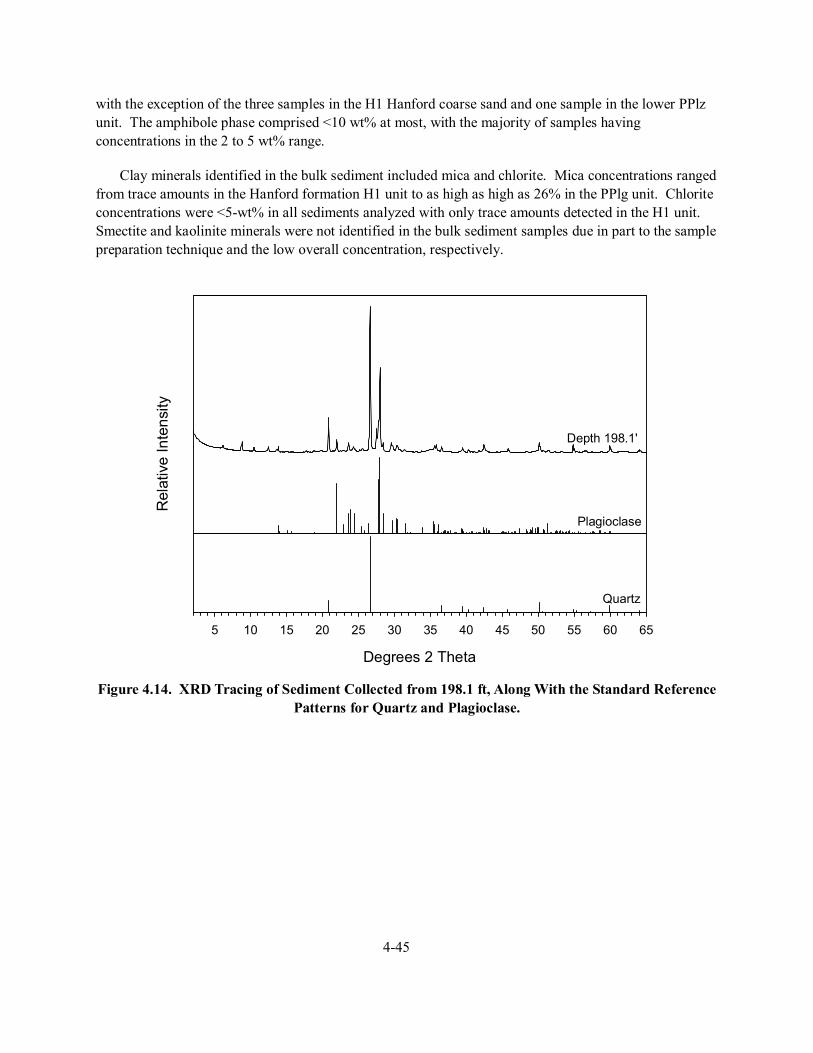
4-45

with the exception of the three samples in the H1 Hanford coarse sand and one sample in the lower PPlz unit. The amphibole phase comprised <10 wt% at most, with the majority of samples having concentrations in the 2 to 5 wt% range.

Clay minerals identified in the bulk sediment included mica and chlorite. Mica concentrations ranged from trace amounts in the Hanford formation H1 unit to as high as high as 26% in the PPlg unit. Chlorite concentrations were <5-wt% in all sediments analyzed with only trace amounts detected in the H1 unit. Smectite and kaolinite minerals were not identified in the bulk sediment samples due in part to the sample preparation technique and the low overall concentration, respectively.

Degrees 2 Theta

5 10 15 20 25 30 35 40 45 50 55 60 65

Rel

ativ

e In

tens

ity

Quartz

Depth 198.1'

Plagioclase

Figure 4.14. XRD Tracing of Sediment Collected from 198.1 ft, Along With the Standard Reference

Patterns for Quartz and Plagioclase.

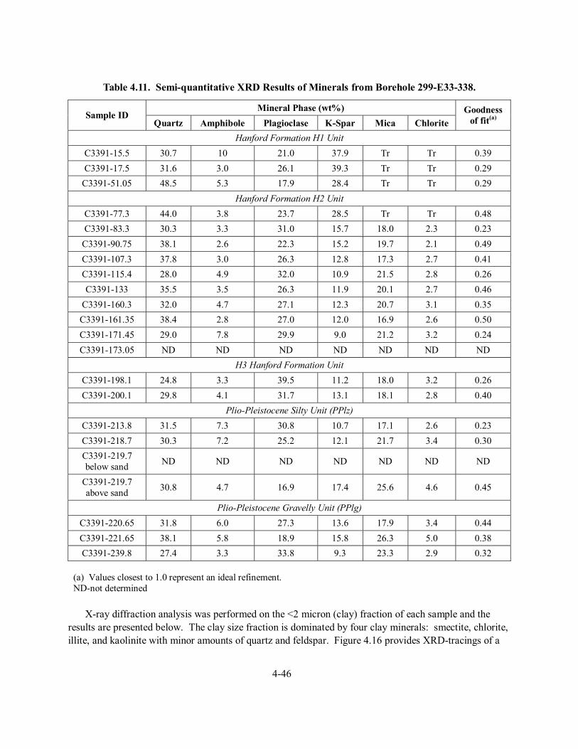
4-46

Table 4.11. Semi-quantitative XRD Results of Minerals from Borehole 299-E33-338.

Mineral Phase (wt%) Sample ID

Quartz Amphibole Plagioclase K-Spar Mica Chlorite Goodness

of fit(a)

Hanford Formation H1 Unit C3391-15.5 30.7 10 21.0 37.9 Tr Tr 0.39 C3391-17.5 31.6 3.0 26.1 39.3 Tr Tr 0.29

C3391-51.05 48.5 5.3 17.9 28.4 Tr Tr 0.29 Hanford Formation H2 Unit

C3391-77.3 44.0 3.8 23.7 28.5 Tr Tr 0.48 C3391-83.3 30.3 3.3 31.0 15.7 18.0 2.3 0.23

C3391-90.75 38.1 2.6 22.3 15.2 19.7 2.1 0.49 C3391-107.3 37.8 3.0 26.3 12.8 17.3 2.7 0.41 C3391-115.4 28.0 4.9 32.0 10.9 21.5 2.8 0.26 C3391-133 35.5 3.5 26.3 11.9 20.1 2.7 0.46

C3391-160.3 32.0 4.7 27.1 12.3 20.7 3.1 0.35 C3391-161.35 38.4 2.8 27.0 12.0 16.9 2.6 0.50 C3391-171.45 29.0 7.8 29.9 9.0 21.2 3.2 0.24 C3391-173.05 ND ND ND ND ND ND ND

H3 Hanford Formation Unit C3391-198.1 24.8 3.3 39.5 11.2 18.0 3.2 0.26 C3391-200.1 29.8 4.1 31.7 13.1 18.1 2.8 0.40

Plio-Pleistocene Silty Unit (PPlz) C3391-213.8 31.5 7.3 30.8 10.7 17.1 2.6 0.23 C3391-218.7 30.3 7.2 25.2 12.1 21.7 3.4 0.30 C3391-219.7 below sand ND ND ND ND ND ND ND

C3391-219.7 above sand 30.8 4.7 16.9 17.4 25.6 4.6 0.45

Plio-Pleistocene Gravelly Unit (PPlg) C3391-220.65 31.8 6.0 27.3 13.6 17.9 3.4 0.44 C3391-221.65 38.1 5.8 18.9 15.8 26.3 5.0 0.38 C3391-239.8 27.4 3.3 33.8 9.3 23.3 2.9 0.32

(a) Values closest to 1.0 represent an ideal refinement. ND-not determined

X-ray diffraction analysis was performed on the <2 micron (clay) fraction of each sample and the

results are presented below. The clay size fraction is dominated by four clay minerals: smectite, chlorite, illite, and kaolinite with minor amounts of quartz and feldspar. Figure 4.16 provides XRD-tracings of a

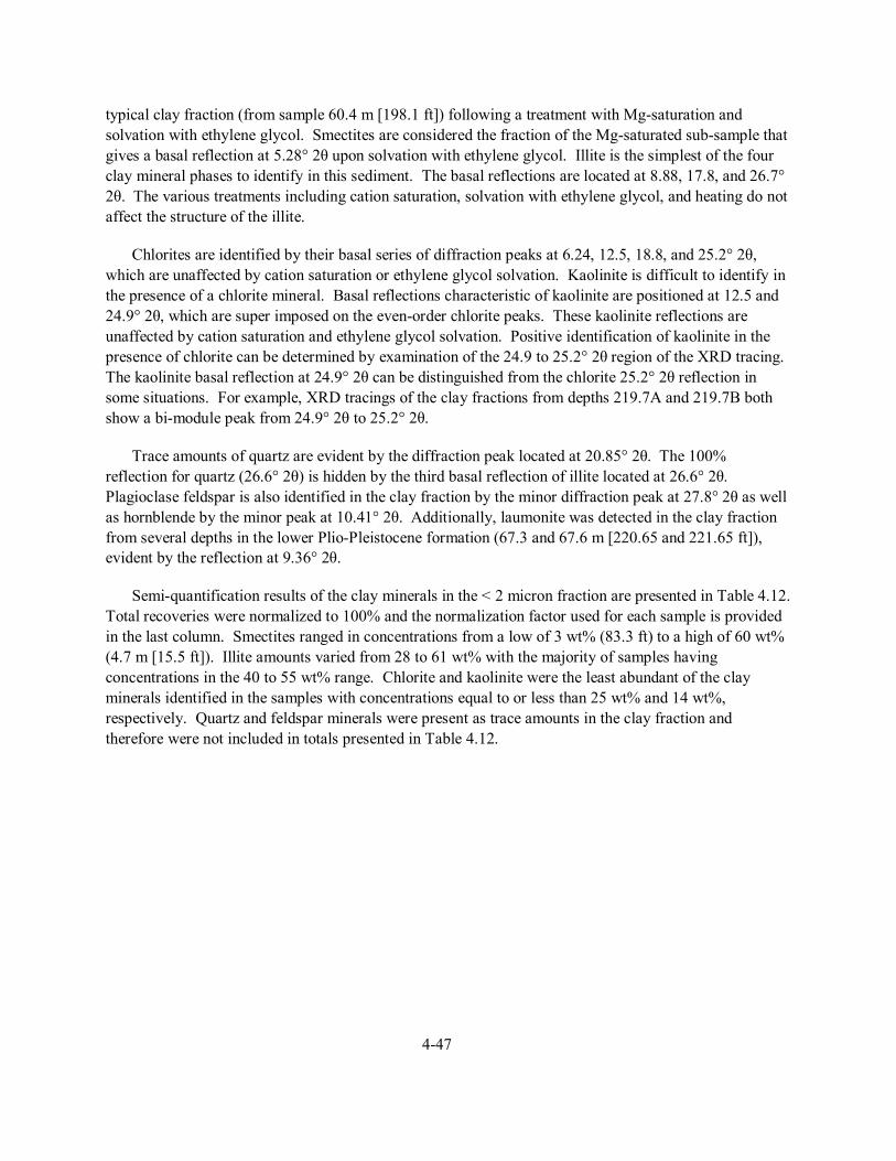
4-47

typical clay fraction (from sample 60.4 m [198.1 ft]) following a treatment with Mg-saturation and solvation with ethylene glycol. Smectites are considered the fraction of the Mg-saturated sub-sample that gives a basal reflection at 5.28° 2θ upon solvation with ethylene glycol. Illite is the simplest of the four clay mineral phases to identify in this sediment. The basal reflections are located at 8.88, 17.8, and 26.7° 2θ. The various treatments including cation saturation, solvation with ethylene glycol, and heating do not affect the structure of the illite.

Chlorites are identified by their basal series of diffraction peaks at 6.24, 12.5, 18.8, and 25.2° 2θ, which are unaffected by cation saturation or ethylene glycol solvation. Kaolinite is difficult to identify in the presence of a chlorite mineral. Basal reflections characteristic of kaolinite are positioned at 12.5 and 24.9° 2θ, which are super imposed on the even-order chlorite peaks. These kaolinite reflections are unaffected by cation saturation and ethylene glycol solvation. Positive identification of kaolinite in the presence of chlorite can be determined by examination of the 24.9 to 25.2° 2θ region of the XRD tracing. The kaolinite basal reflection at 24.9° 2θ can be distinguished from the chlorite 25.2° 2θ reflection in some situations. For example, XRD tracings of the clay fractions from depths 219.7A and 219.7B both show a bi-module peak from 24.9° 2θ to 25.2° 2θ.

Trace amounts of quartz are evident by the diffraction peak located at 20.85° 2θ. The 100% reflection for quartz (26.6° 2θ) is hidden by the third basal reflection of illite located at 26.6° 2θ. Plagioclase feldspar is also identified in the clay fraction by the minor diffraction peak at 27.8° 2θ as well as hornblende by the minor peak at 10.41° 2θ. Additionally, laumonite was detected in the clay fraction from several depths in the lower Plio-Pleistocene formation (67.3 and 67.6 m [220.65 and 221.65 ft]), evident by the reflection at 9.36° 2θ.

Semi-quantification results of the clay minerals in the < 2 micron fraction are presented in Table 4.12. Total recoveries were normalized to 100% and the normalization factor used for each sample is provided in the last column. Smectites ranged in concentrations from a low of 3 wt% (83.3 ft) to a high of 60 wt% (4.7 m [15.5 ft]). Illite amounts varied from 28 to 61 wt% with the majority of samples having concentrations in the 40 to 55 wt% range. Chlorite and kaolinite were the least abundant of the clay minerals identified in the samples with concentrations equal to or less than 25 wt% and 14 wt%, respectively. Quartz and feldspar minerals were present as trace amounts in the clay fraction and therefore were not included in totals presented in Table 4.12.

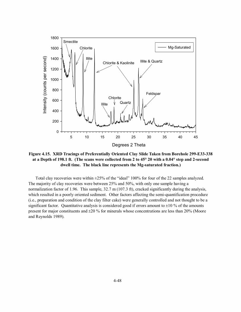
4-48

Degrees 2 Theta

5 10 15 20 25 30 35 40 45

Inte

nsity

(cou

nts

per s

econ

d)

0

200

400

600

800

1000

1200

1400

1600

1800

Mg-SaturatedSmectite

Chlorite

Chlorite

Illite

Illite

Chlorite & Kaolinite Illite & Quartz

Quartz

Feldspar

Figure 4.15. XRD Tracings of Preferentially Oriented Clay Slide Taken from Borehole 299-E33-338

at a Depth of 198.1 ft. (The scans were collected from 2 to 45° 2θ with a 0.04° step and 2-second dwell time. The black line represents the Mg-saturated fraction.)

Total clay recoveries were within ±25% of the “ideal” 100% for four of the 22 samples analyzed.

The majority of clay recoveries were between 25% and 50%, with only one sample having a normalization factor of 1.96. This sample, 32.7 m (107.3 ft), cracked significantly during the analysis, which resulted in a poorly oriented sediment. Other factors affecting the semi-quantification procedure (i.e., preparation and condition of the clay filter cake) were generally controlled and not thought to be a significant factor. Quantitative analysis is considered good if errors amount to ±10 % of the amounts present for major constituents and ±20 % for minerals whose concentrations are less than 20% (Moore and Reynolds 1989).

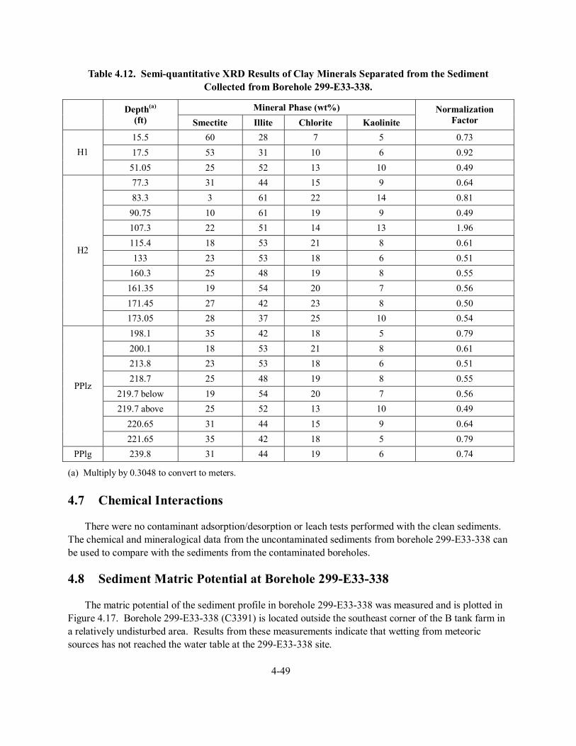
4-49

Table 4.12. Semi-quantitative XRD Results of Clay Minerals Separated from the Sediment Collected from Borehole 299-E33-338.

Mineral Phase (wt%) Depth(a)

(ft) Smectite Illite Chlorite Kaolinite Normalization

Factor

15.5 60 28 7 5 0.73 17.5 53 31 10 6 0.92 H1

51.05 25 52 13 10 0.49 77.3 31 44 15 9 0.64 83.3 3 61 22 14 0.81

90.75 10 61 19 9 0.49 107.3 22 51 14 13 1.96 115.4 18 53 21 8 0.61 133 23 53 18 6 0.51

160.3 25 48 19 8 0.55 161.35 19 54 20 7 0.56 171.45 27 42 23 8 0.50

H2

173.05 28 37 25 10 0.54 198.1 35 42 18 5 0.79 200.1 18 53 21 8 0.61 213.8 23 53 18 6 0.51 218.7 25 48 19 8 0.55

219.7 below 19 54 20 7 0.56 219.7 above 25 52 13 10 0.49

220.65 31 44 15 9 0.64

PPlz

221.65 35 42 18 5 0.79 PPlg 239.8 31 44 19 6 0.74

(a) Multiply by 0.3048 to convert to meters. 4.7 Chemical Interactions

There were no contaminant adsorption/desorption or leach tests performed with the clean sediments. The chemical and mineralogical data from the uncontaminated sediments from borehole 299-E33-338 can be used to compare with the sediments from the contaminated boreholes.

4.8 Sediment Matric Potential at Borehole 299-E33-338

The matric potential of the sediment profile in borehole 299-E33-338 was measured and is plotted in Figure 4.17. Borehole 299-E33-338 (C3391) is located outside the southeast corner of the B tank farm in a relatively undisturbed area. Results from these measurements indicate that wetting from meteoric sources has not reached the water table at the 299-E33-338 site.

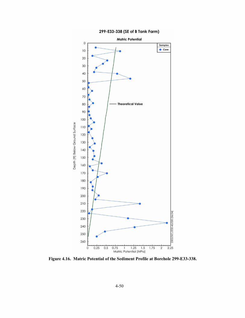
4-50

Figure 4.16. Matric Potential of the Sediment Profile at Borehole 299-E33-338.

5-1

5.0 Summary and Conclusions

Sediment cores from borehole 299-E33-338 near the B-BX-BY WMA have been characterized to establish lithological and geochemical baseline profiles that can be used to support ongoing field investigations concerned with past single shell tank fluid leak events in the vadose zone being conducted by CH2M Hill Hanford Group Inc. The base line results in this report will serve as a “clean sediment” standard for comparison with sediment cores extracted from areas of known contamination within the B-BX-BY WMA. These results will not only help support our understanding of the degree and extent of contamination within the B-BX-BY WMA, but also possible mechanisms associated with fate and transport and risk based assessments of problematic contaminants such as technetium-99 and uranium.

The geology under the B-BX-BY WMA forms the framework through which the contaminants move, and as discussed in Serne et. al. 2002, provides the basis with which to interpret and extrapolate the physical and geochemical properties that control the migration and distribution of contaminants. Specifically, the identification of major lithological contacts and the interrelationships between the coarser- and finer-grained sediment facies are essential when combined with the geochemical profile for interpreting contaminant behavior in the subsurface. For this borehole, lithologic sections were constructed using detailed geologic descriptions, core photos, and geophysical logs. In some cases, the results of laboratory analyses (e.g. particle-size distribution, moisture, calcium carbonate content) helped refine the resulting stratigraphic and lithological interpretations.

Our conceptual model of the vadose zone associated with the 299 E33-338 borehole involves five distinct stratigraphic units beginning with the Hanford formation H1 unit from the surface to a depth of approximately 15.7 m (approximately 51.5-ft) described as a sandy gravel to gravelly sand sequence. This is followed by the Hanford formation H2 unit extending to a depth of approximately 57.9 m (109 ft) that is a sand sequence consisting of sand dominated facies, with multiple graded beds of horizontal to tabular cross-bedd sand to slightly gravelly sand. These graded beds are sometimes capped with thin layers of silty sand to silt. The last unit associated with the cataclysmic flood deposits is the Hanford H3 formation unit that extends to a depth of approximately 64.8 m (212.5 ft). It is a gravelly sand to slightly gravelly sand sequence. Just below the H3 unit is the Plio-Pleistocene silty unit (PPlz) extending to a depth of approximately 67.8 m (222.4 ft). This unit is a silt-dominated sequence consisting of interstratified well sorted silt and fine sand. The last unit characterized from this borehole was the Plio-Pleistocene gravelly unit (PPlg) extending to a depth of approximately 82.6 m (271 ft), however sampling ended at approximately 73.1 m (239.8 ft). This unit is differentiated from the PPlz due to its sandy gravel to gravelly sand sequence consisting predominantly of unconsolidated basalt-rich sand and gravel.

Sediment samples from the various stratigraphic unites were analyzed and characterized in the laboratory for the following parameters:

• Mass Water Content • Soil Suction • Particle-Size Distribution

5-2

• Calcium Carbonate and Organic Carbon Contents • Bulk Chemical Composition • Mineralogy • Water Leach (1:1 sediment to water extraction) • Acid Leach (8M nitric acid extraction) Physical properties, such as particle size distribution and water content varied according to lithology

as expected. In general, elevated areas of water content (~ >5%) were typically associated with regions of fine grain sediments. Most notable are those regions involving lithological facies at which water contents equal or exceed 10%. Three major peaks are noted at 15.7, 52.9, and 67.1 m (51.6, 173.6, and 220.2 ft) bgs with water contents of 12.95, 14.27, and 26.02% respectively. Along with water content, soil suction measurements were made on most of the core liner and grab samples from the borehole using the filter paper method. Three major peaks were noted approximately 14, 64, and 73 m (45, 210, and 240 ft) bgs with suction measurements of approximately 1.3, 1.5, and 2.2 Mpa. The matric potential profile indicates that wetting from meteoric water has not reached the water table.

The semi-quantitative mineral composition for the bulk sediments characterized in the H1 unit and the first samples associated with the H2 unit (23.7 m [77.8 ft] bgs) consisted mostly of quartz (30.7 to 31.6 wt%), plagioclase (21.0 to 26.1 wt%) , potassium feldspars (28.4 to 39.3 wt%), amphibole (3.0 to 10.0 wt%), with trace amounts of mica and chlorite. The remaining H2, H3, PPlz, and PPlg units (below 25.5 m [83.8 ft] bgs down to 73.2 [240.3 ft] bgs) were similar consisting of quartz (24.8 to 38.8 wt%), plagioclase (17.9 to 33.8 wt%), amphibole (2.8 to 7.8 wt%), potassium feldspars (9.0 to 15.8 wt%), mica (17.1 to 25.6 wt%), and chlorite (2.1 to 4.6 wt%). The particle density for the sediments ranged from 2.57 to 2.79 g/cm3.

Inorganic carbon results reported in terms of calcium carbonate were found to be within the range of 0.5 to 2.0 wt %, and are consistent with results reported elsewhere (e.g. Serne et. al. 2002). The method used to measure the organic carbon relies on subtracting the inorganic carbon from the total carbon in the sample; for such low carbon values this method is not very accurate. The low values for organic carbon (0.01 to 0.14 %) are within the ranges generally reported for sediment at the Hanford site.

Bulk sediment samples were characterized for major and trace elements using a lithium metaborate/tetraborate fusion procedure, and then analyzed by inductively coupled plasma –optical emission spectroscopy (ICP-OES) and ICP-MS methods. Overall results showed very little difference in the primary elemental oxide concentrations for any of the sediment samples as a function of depth or lithology. The primary elemental oxides in decreasing concentration include SiO2 (58.77 to 70.33 wt%), Al2O3 (12.7 to 15.73 wt%), Fe2O3 (3.74 to 7.92 wt%), CaO (3.02 to 4.80 wt%), Na2O (2.05 to 3.23 wt%), K2O (1.70 to 2.65 wt%), MgO (1.64 to 2.73 wt%), TiO2 (0.51 to 1.39 wt%), P2O5 (0.13 to 0.30 wt%), and MnO (0.07 to 0.12 wt%). The additional 35 trace elements reported for each sample in terms of µg/g of dry sediment showed little, if any, significant variation in concentration.

5-3

The water chemistry analysis for samples collected between 5 and 73 m (16 and 240 ft) bgs using the 1:1 soil to water extract method shows no strong trends as a function of depth and there is little, if any, indication of tank waste interaction with vadose zone soils at this location. Primary characteristics include the following:

• The 1:1 sediment-to-water extract pH varied from 6.97 to 7.74 and in general increased with depth with an average value of 7.4 (Figure 4.9 and Table 4.3).

• There were small increases in pH at the contact between the Hanford H2 and H3 units and the top and bottom of the Plio-Pleistocene mud unit.

• Porewater EC (dilution corrected) varied from 0.88 to 4.3 mS/cm with an average of 2.4 mS/cm.

• There were high EC values deep in the Hanford H2 unit at approximately 49 m (160 ft) bgs and in the deepest sample characterized (i.e., in the PPlg).

The shapes of the major cation profiles (sodium, potassium, calcium, magnesium, and strontium) in terms of calculated porewater concentration versus depth are very similar with slight peaks in the deep portion of the H2 unit at approximately 49 m (160 ft) bgs, at the top of the Plio-Pleistocene silty unit, and in the deepest sample characterized in the PPlg unit. All three of these samples had very low water contents and thus the dilution factor was high. The apparent high porewater concentrations likely represent some dissolution of salts from the sediment that are multiplied by a large dilution factor, and thus suggest more saline porewater than surrounding sediments with higher water content. In general, the calculated porewater cation concentrations ranged from 63 to 275, 11 to 138, 11 to 56, and 70 to 558 mg/L for calcium, potassium, magnesium, and sodium, respectively. The averages and median values were (142, 149), (60, 58), (34, 38), and (190, 141) mg/L, for calcium, potassium, magnesium, and sodium, respectively. These values are likely somewhat artificially elevated because of the water extraction of soluble salts along with the porewater.

The calculated porewater concentrations for aluminum, barium, iron, silicon, and uranium-238 were also evaluated. The porewater concentrations ranged from 0.01 to 5.29, 0.0 to 6.4, and 46 to 350 mg/L for aluminum, barium, and iron, respectively, and 1.8 to 24 µg/L for uranium. The uncontaminated uranium-238 porewater concentration is especially important for comparison with contaminated borehole sediment porewaters.

The shapes of the major anion profiles (fluoride, chloride, nitrate, bicarbonate, phosphate, and sulfate) in terms of calculated porewater concentration versus depth showed no consistent depths where all anions peaked unlike the major cation profiles. The wetter samples do consistently show low calculated porewater anion concentrations suggesting that the dilution factor is again controlling the apparent concentrations. That is, all the sediments likely dissolve some salts that are not truly in the porewater, so that the dilution correction makes it appear that the porewater anion concentrations are higher in the drier sediments. The calculated porewater anion concentrations range from 0.4 to 23.3, 1.8 to 223, 1.3 to 100, 296 to 1877, and 196 to 117 mg/L for fluoride, chloride, nitrate, bicarbonate, and sulfate, respectively. The average and median values are (6.3, 4.8), (35, 19), (19, 10), (993, 1030), and (196, 117) mg/L for

5-4

fluoride, chloride, nitrate, bicarbonate, and sulfate, respectively. These values are likely somewhat artificially elevated because of the water extraction of soluble salts.

The mass of several constituents per gram of dry sediment that were leached by water and acid extracts are shown in Figures 4.13 and 4.14. In all cases, the mass that was water leachable is a very small fraction of the mass that was acid extractable. These concentrations can be compared with the same constituents for contaminated sediments to get an estimate of the mass of a constituent present in the vadose zone profile after contact with tank leaked liquids.

6-1

6.0 References

American Society of Agronomy (ASA). 1986a. “Gravimetry with Oven Drying,” Chapter 21-2.2 in Methods of Soil Analysis-Part 1, 2nd edition of Physical and Mineralogical Methods, SSSA Book Series No. 5, ed. A Klute, pp. 503-507. Soil Science Society of America, Madison, Wisconsin.

American Society of Agronomy (ASA). 1986b. “Hydrometer Method.” Chapter 15-5 in Methods of Soil Analysis-Part 1, 2nd edition of Physical and Mineralogical Methods, SSSA Book Series No. 5, ed. A Klute, pp. 404-408. Soil Science Society of America, Madison, Wisconsin.

American Society of Agronomy (ASA). 1986c. “Pynchnometer Method.” Chapter 14-3 in Methods of Soil Analysis-Part 1, 2nd Edition of Physical and Mineralogical Methods, SSSA Book Series No. 5, ed .A Klute, pp. 378-379. Soil Science Society of America, Madison, Wisconsin.

American Society of Agronomy (ASA). 1996. Methods of Soil Analysis-Part 3, Chemical Methods, SSSA Book Series 5, ed. DL Sparks. Soil Science Society of America, Madison, Wisconsin.

American Society for Testing and Materials (ASTM) D4129-88. 1988. Standard Test Method for Total and Organic Carbon in Water by High Temperature Oxidation and by Coulometric Detection. American Society for Testing and Materials, West Conshohocken, Pennsylvania.

American Society for Testing and Materials (ASTM) D2488-93. 1993. Standard Practice for Description and Identification of Soils (Visual-Manual Procedure). American Society for Testing and Materials, West Conshohocken, Pennsylvania.

Baker, VR, BN Bjornstad, AJ Busacca, KR Fecht, EP Kiver, UL Moody, JG Rigby, DF Stradling, and AM Tallman. 1991. “Quanternary Geology of the Columbia Plateau”. In Morisson, RB ed., Quaternary Nonglacial Geology. Conterminous U. S. Geology of North America, Boulder, Colorado, Geol. Soc. Am. K-2:215-250.

Bjornstad BN, KR Fecht, and CJ Pluhar. 2001. “Long history of Pre-Wisconsin, Ice Age Cataclysmic Floods: Evidence from Southeastern Washington State.” Journal of Geology, v. 109, p. 695-713.

Brindley GW and G Brown, eds. 1980 . Crystal Structures of Clay Minerals and Their X-Ray Identification. Monograph No. 5, Mineralogical Society, London.

Caggiano JA. 1996. Assessment Groundwater Monitoring Plan for Single Shell Tank Waste Management Area B-BX-BY. WHC-SD-ENV-AP-002, Westinghouse Hanford Company, Richland, Washington.

Caggiano JA and SM Goodwin. 1991. Interim Status Groundwater Monitoring Plan for the Single-Shell Tanks. WHC-SD-EN-AP-012, Westinghouse Hanford Company, Richland, Washington.

CH2M HILL. 2000. Site Specific SST Phase 1 RFI/CMS Work Plan Addendum for WMA B-BX-BY. RPP-6072, Rev. 1, CH2M HILL Hanford Group, Inc. Richland, Washington.

6-2

Connelly MP, BH Ford, JW Lindberg, SJ Trent, CD Delaney, and JV Borghese. 1992. Hydrogeologic Model for the 200 East Groundwater Aggregate Area. WHC-SD-EN-TI-019, Westinghouse Hanford Company, Richland, Washington.

Deka RN, M Wairiu, PW Mtakwa, CE Mullins, EM Veenendaal, and J Towend. 1995. “Use and Accuracy of the Filter Paper Method for Measuring Soil Matric Potential,” European J. of Soil Sci. 46:233-238.

DOE. 1999. Phase 1 RCRA Facility Investigation/Corrective Measures Study Work Plan for the SST Waste Management Areas. DOE/RL-99-36, Rev. 0, U.S. Department of Energy, Richland Operations Office, Richland, Washington.

Drever JI. 1973. “The Preparation of Oriented Clay Mineral Specimens for X-Ray Diffraction Analysis by a Filter-Membrane Peel Technique.” Amer. Minerl. 58:553-554.

EPA Method 3050B. 2000a. “Acid Digestion of Sediments, Sludges, and Soils.” Test Methods for Evaluating Solid Waste, Physical/Chemical Methods. EPA Publication SW-846, available online http://www.epa.gov/epaoswer/hazwaste/test/sw846.htm

EPA Method 6010B. 2000b. “Inductively Coupled Plasma-Atomic Emission Spectrometry.” Test Methods for Evaluating Solid Waste, Physical/Chemical Methods. EPA Publication SW-846, available online http://www.epa.gov/epaoswer/hazwaste/test/sw846.htm

EPA Method 6020. 2000c. “Inductively Coupled Plasma-Mass Spectrometry.” Test Methods for Evaluating Solid Waste, Physical/Chemical Methods. EPA Publication SW-846, available online http://www.epa.gov/epaoswer/hazwaste/test/sw846.htm

Folk RL. 1968. Petrology of Sedimentary Rocks. Hemphill, Austin, Texas.

Horton DG. 2002. Borehole Data Package for Calendar Year 2001 RCRA Wells at Single-Shell Tank Waste Management Area B-BX-BY. PNNL-13827, Pacific Northwest National Laboratory, Richland, Washington.

Jackson ML. 1969. Soil Chemical Analysis – Advanced Course—2nd Edition. Department of Soil Science, University of Wisconsin, Madison, Wisconsin.

Last GV, BN Bjornstad, MP Bergeron, DW Wallace, DR Newcomer, JA Schramke, MA Chamness, CS Cline, SP Airhart, and JS Wilbur. 1989. Hydrogeology of the 200 Areas Low-Level Burial Grounds - An Interim Report. PNL-6820, 2 volumes, Pacific Northwest Laboratory, Richland, Washington.

Lindsey KA, SE Kos, and KD Reynolds. 2000. Vadose Zone Geology of Boreholes 299-W22-50 and 299-W23-19 S-SX Waste Management Area, Hanford Site, South-Central Washington. RPP-6149, Rev. 0, Waste Management Technical Services, Richland, Washington.

6-3

Lindsey KA, SE Kos, and KD Reynolds. 2001. Vadose Zone Geology of Boreholes 299-E33-45 and 299-E33-46 B-BX-BY Waste Management Area, Hanford Site, South-Central Washington. RPP-8681, Rev. 0, prepared for the Office of River Protection by CH2M Hill Hanford Group, Inc., Richland, Washington.

Lindsey KA, BN Bjornstad, JW Lindberg, and KM Hoffman. 1992. Geologic setting of the 200 East Area: An update. WHC-SD-EN-TI-012, Westinghouse Hanford Company, Richland, Washington.

Lindsey KA, SP Reidel, KR Fecht, JL Slate, AG Law, and AM Tallman. 1994. "Geohydrologic Setting of the Hanford Site, South-Central Washington." In Geologic Field Trips in the Pacific Northwest. eds. DA Swanson and RA Hagerud, pp. 1C-1 to 1C-16. Geological Society of America Meeting, Geological Society of America, Boulder, Colorado.

Moore DM and RC Reynolds, Jr. 1989. X-Ray Diffraction and the Identification and Analysis of Clay Minerals. Oxford University Press, New York.

Nabutovskih SM. 1998. Results of Phase I Groundwater Quality Assessment for Single Shell Tank Waste Management Areas B-BX-BY as the Hanford Site. PNNL-11826, Pacific Northwest National Laboratory, Richland, Washington.

Newman ACD, ed. 1987. Chemistry of Clays and Clay Minerals. Monograph No 6, Mineralogical Society, London, England.

Price WH and KR Fecht. 1976. Geology of the 241-B Tank Farm. ARH-LD-129, Atlantic Richfield Hanford Company, Richland, Washington.

PSPL. 1982. Skagit/Hanford Nuclear Project, Preliminary Safety Analysis Report. Vol. 4. Appendix 20. Amendment 23. Puget Sound Power and Light Company. Bellevue, Washington.

Reidel SP and KR Fecht. 1994. Geologic Map of the Priest Rapids 1:100,000 Quadrangle, Washington. Washington Division of Geology and Earth Resources Open-File Report 94-13, 22 p.

Resource Conservation and Recovery Act of 1976, 42 U.S.C. 6901, et seq.

Rhoades JD. 1996. “Salinity: Electrical Conductivity and Total Dissolved Solids.” In Methods of Soil Analysis Part 3, JM Bigham ed., pp. 417-435. American Society of Agronomy, Madison, Wisconsin.

Serne RJ, BN Bjornstad , HT Schaef, BA Williams, DC Lanigan, DG Horton, RE Clayton, AV Mitroshkov, VL LeGore , MJ O’Hara, CF Brown , KE Parker, IV Kutnyakov , JN Serne, GV Last, SC Smith, CW Lindenmeier, JM Zachara, and DS Burke. 2002. Characterization of Uncontaminated Vadose Zone Sediment from the Hanford Reservation – RCRA Borehole Core Samples and Composite Samples. PNNL-13757-1, Pacific Northwest National Laboratory, Richland, Washington.

Slate JL. 1996. "Buried Carbonate Paleosols Developed in Pliocene-Pleistocene Deposits of the Pasco Basin, South-Central Washington." USA: Quaternary International, Vol. 34-36, pp. 191-196.

6-4

Slate JL. 2000. Nature and Variability of the Plio-Pleistocene Unit in the 200 West Area of the Hanford Site. BHI-01203, Rev. 0, Bechtel Hanford, Inc., Richland, Washington.

Tallman AM, KR Fecht, MC Marratt, and GV Last. 1979. Geology of the Separations Areas, Hanford Site, South-Central Washington. RHO-ST-23, Rockwell Hanford Operations, Richland, Washington.

US Department of Energy (DOE). 1988. Consultation Draft Site Characterization Plan. DOE/RL-0164, 9 volumes, Richland, Washington.

US Department of Energy (DOE). 1999a. Vadose Zone Characterization Project at the Hanford Tank Farms: B Tank Farm Report, GJO-HAN-28, prepared by U.S. Department of Energy Grand Junction Office for U.S. Department of Energy, Richland Operations Office, Richland, Washington.

US Department of Energy (DOE). 1999b. Vadose Zone Characterization Project at the Hanford Tank Farms: Tank Summary Data Report for Tank B-110. GJ-HAN-131, prepared by U.S. Department of Energy Grand Junction Office for U.S. Department of Energy Office of River Protection, Richland, Washington.

United States Geological Survey (USGS). 2001. “Alkalinity and Acid Neutralizing Capacity.” National Field Manual for the Collection of Water-Quality Data. Available online at http//water.usgs.gov/owq/FieldManual/Chapter6/6.6-contents.html

Wentworth CK. 1922. “A Grade Scale and Class Terms for Clastic Sediments.” Journal of Geology, Vol. 30, p. 377-392.

Wood MI, TE Jones, R Schalla, BN Bjornstad, and SM Narbutovskih. 2000. Subsurface Conditions Description of the B-BX-BY Waste Management Area. HNF-5507, Rev. 0, CH2M HILL Hanford Group, Inc., Richland, Washington.

Appendix A

Summary of Field Geologists’ Sample Descriptions for Borehole 299-E33-338

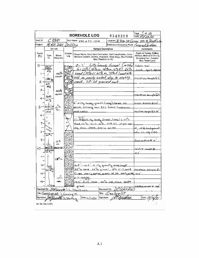
A.1

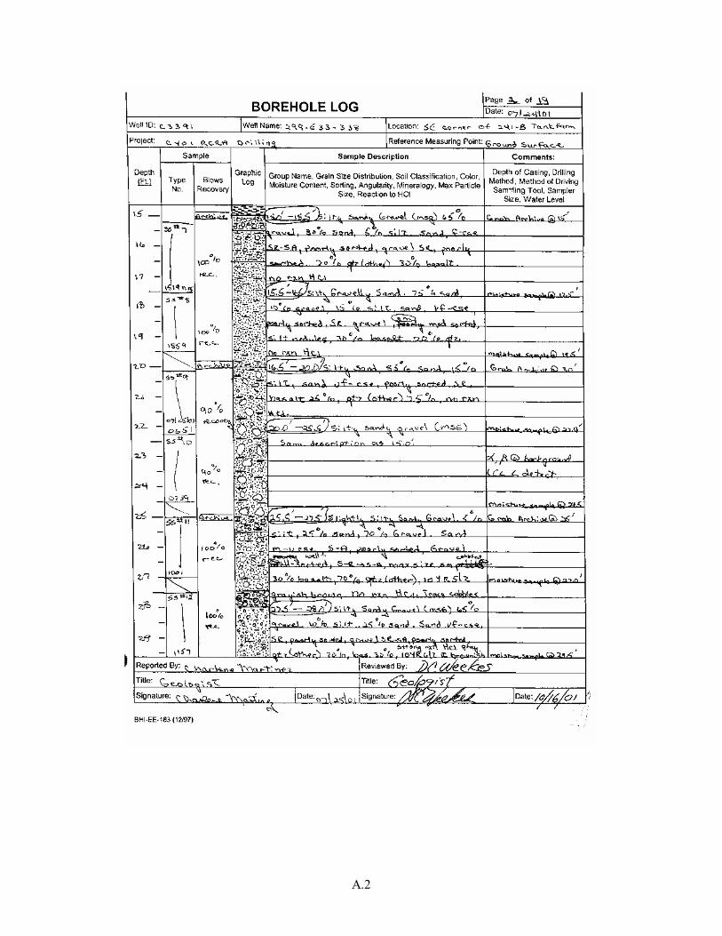
A.2

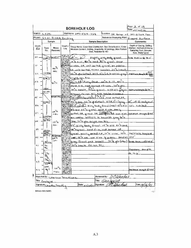
A.3

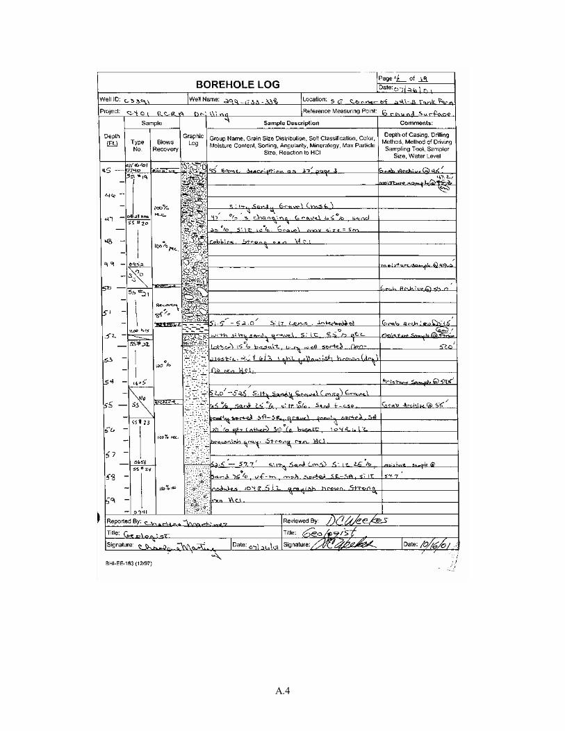
A.4

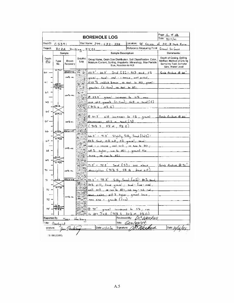
A.5

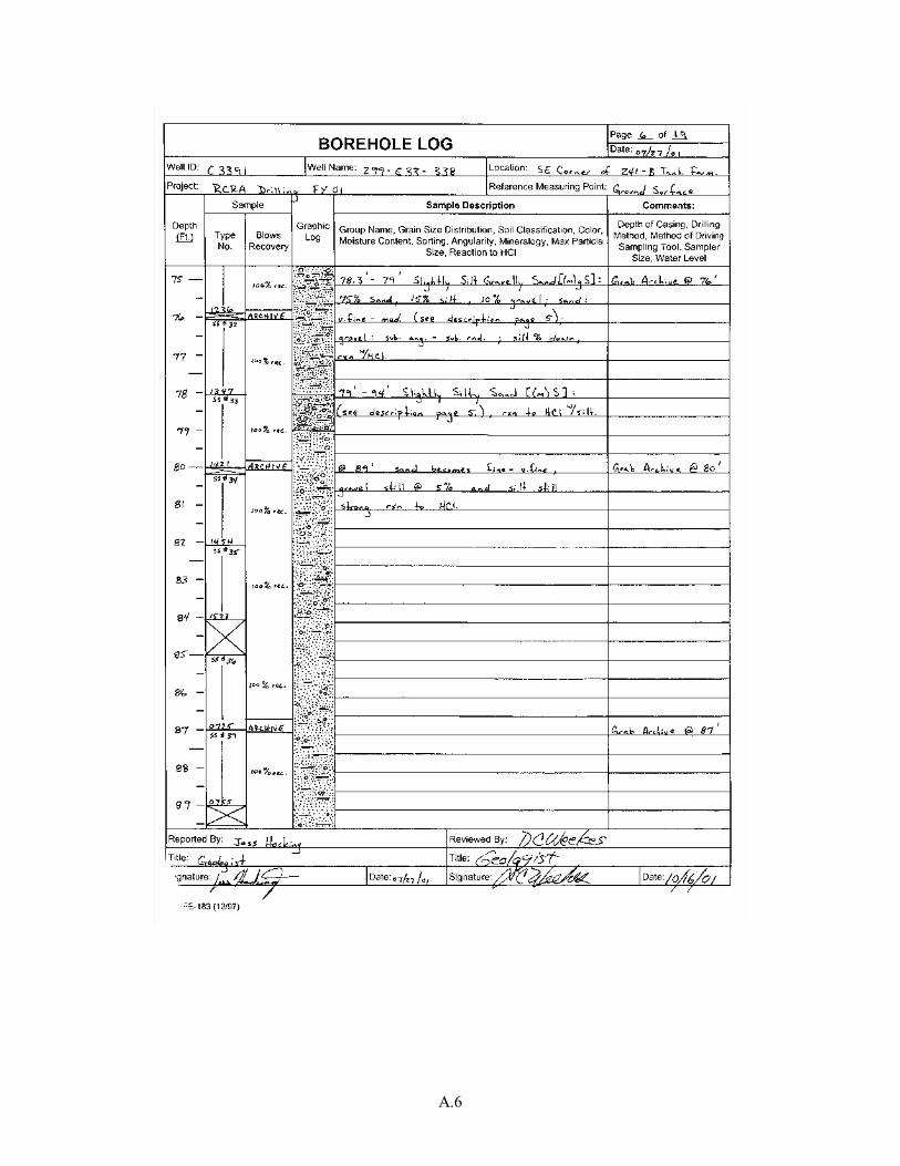
A.6

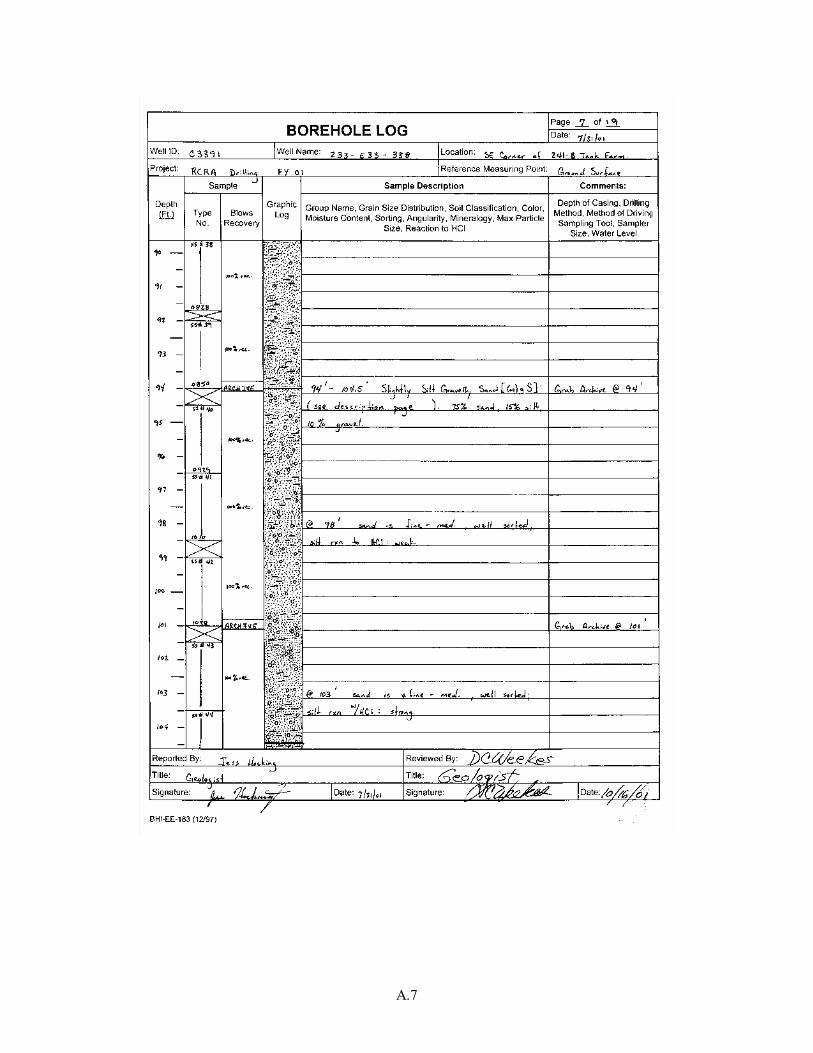
A.7

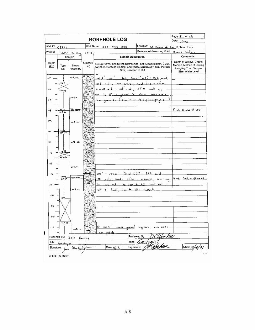
A.8

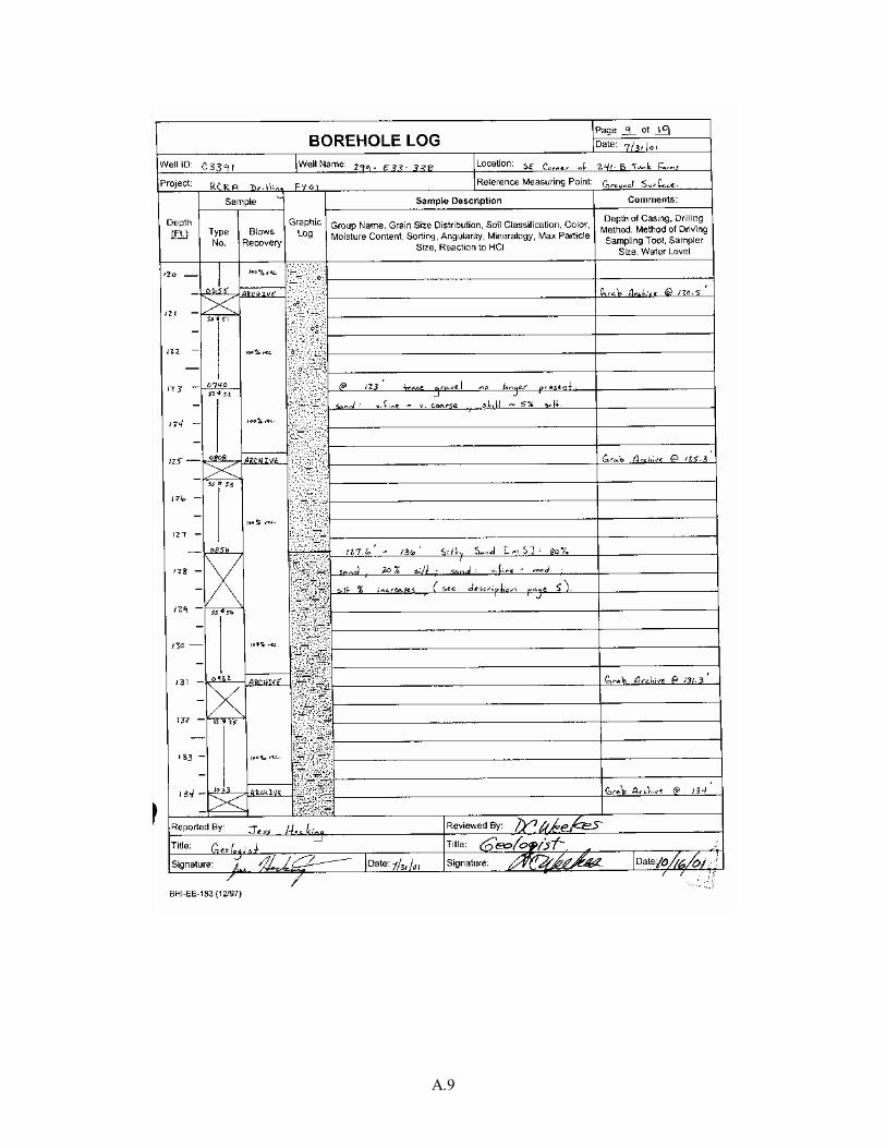
A.9

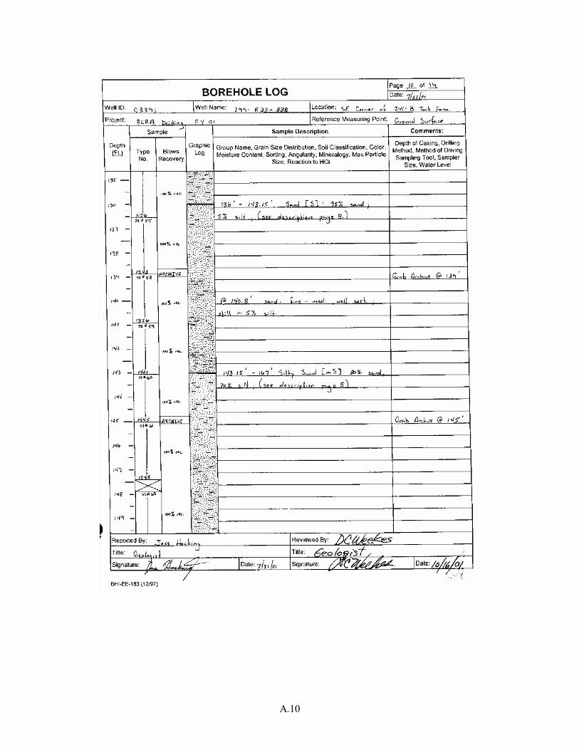
A.10

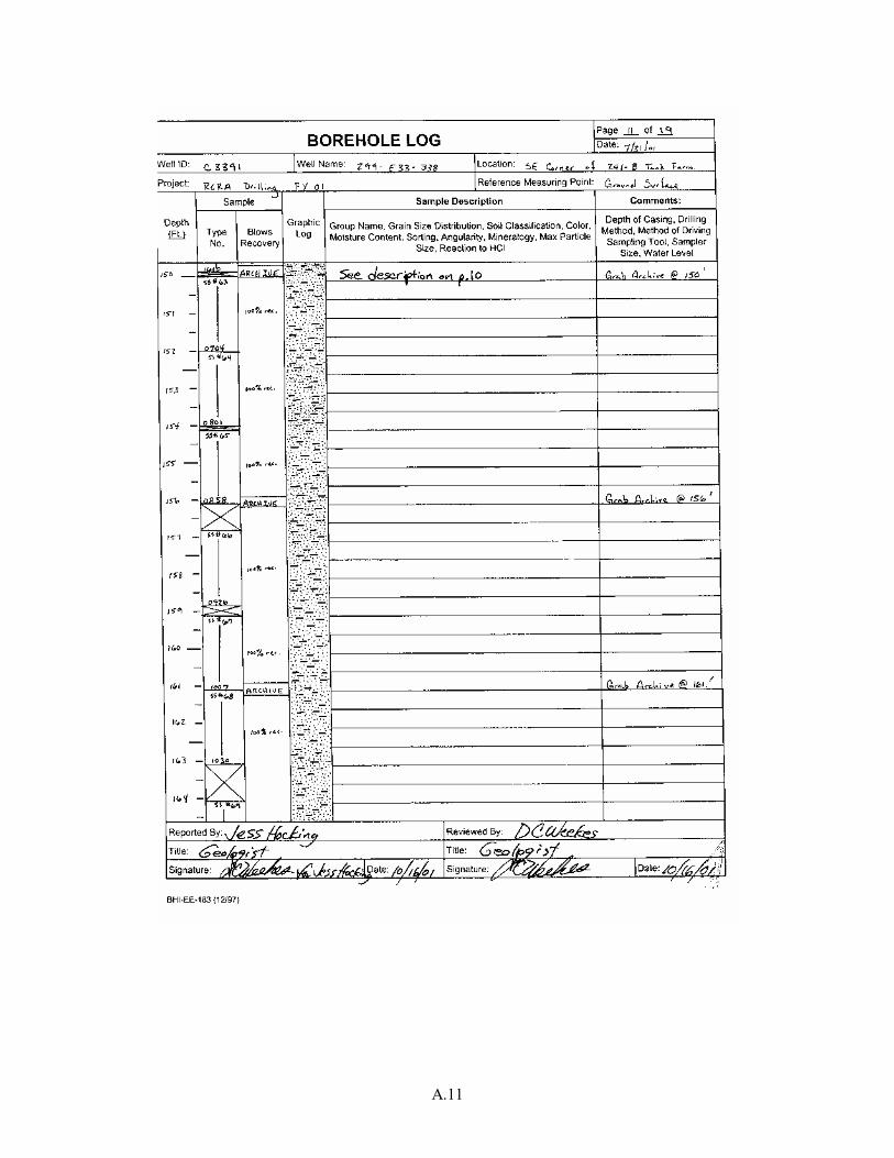
A.11

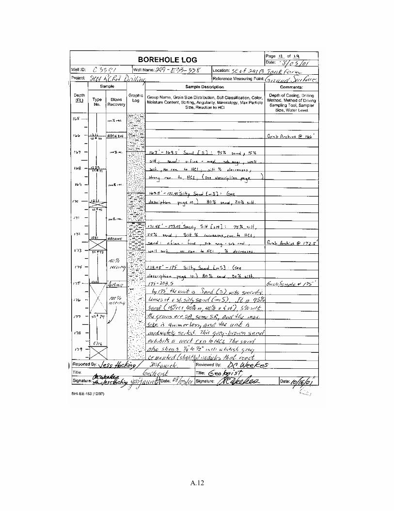
A.12

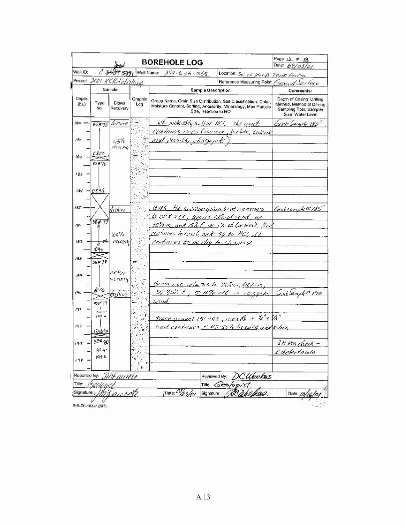
A.13

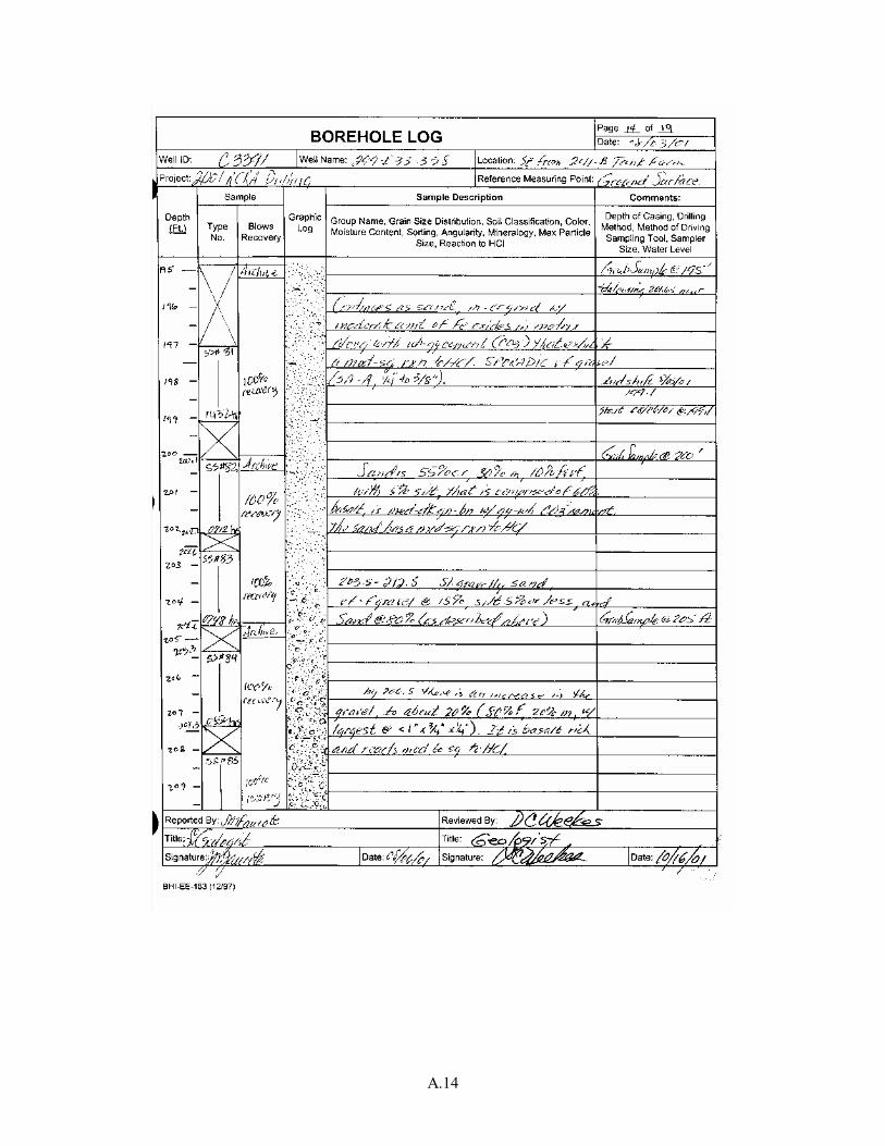
A.14

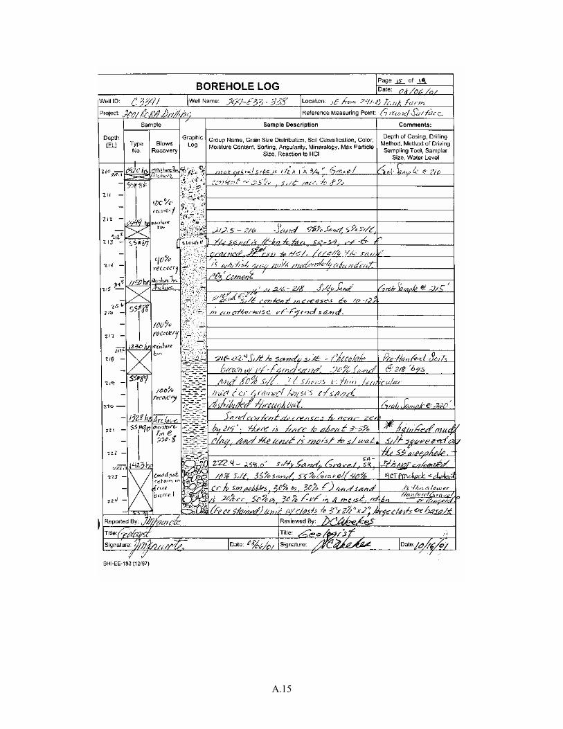
A.15

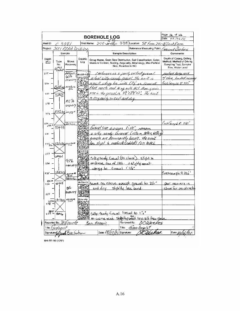
A.16

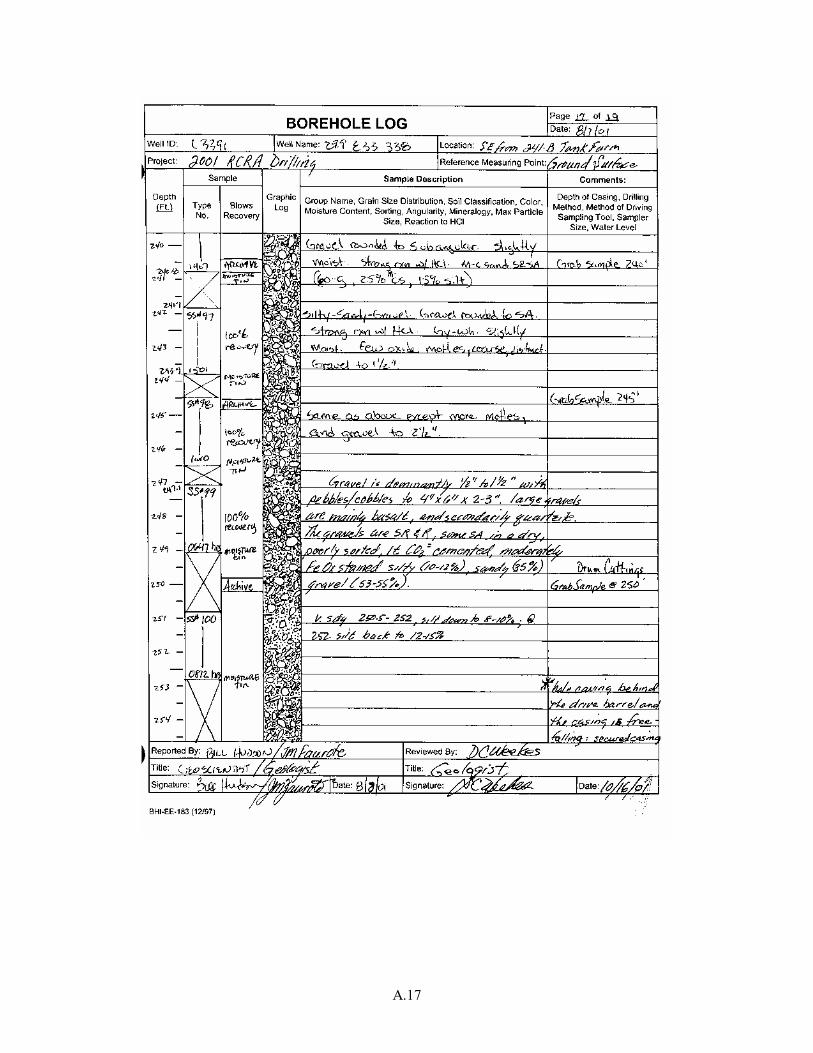
A.17

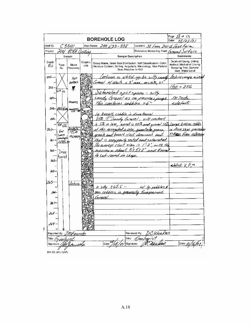
A.18

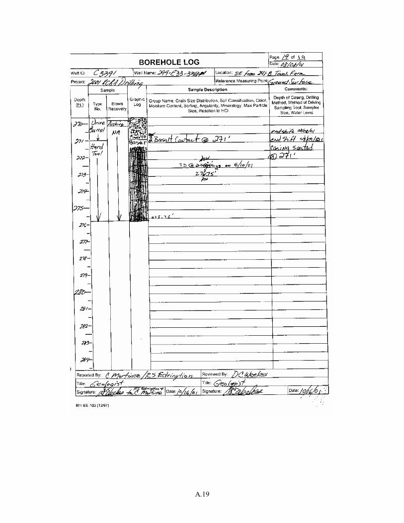
A.19

Appendix B

Summary of Geologists’ Core Sample Descriptions From Borehole 299-E33-338

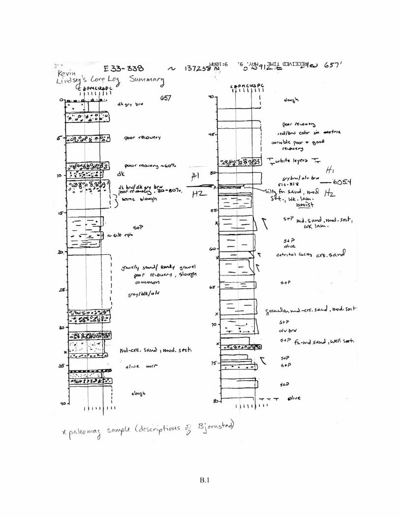
B.1

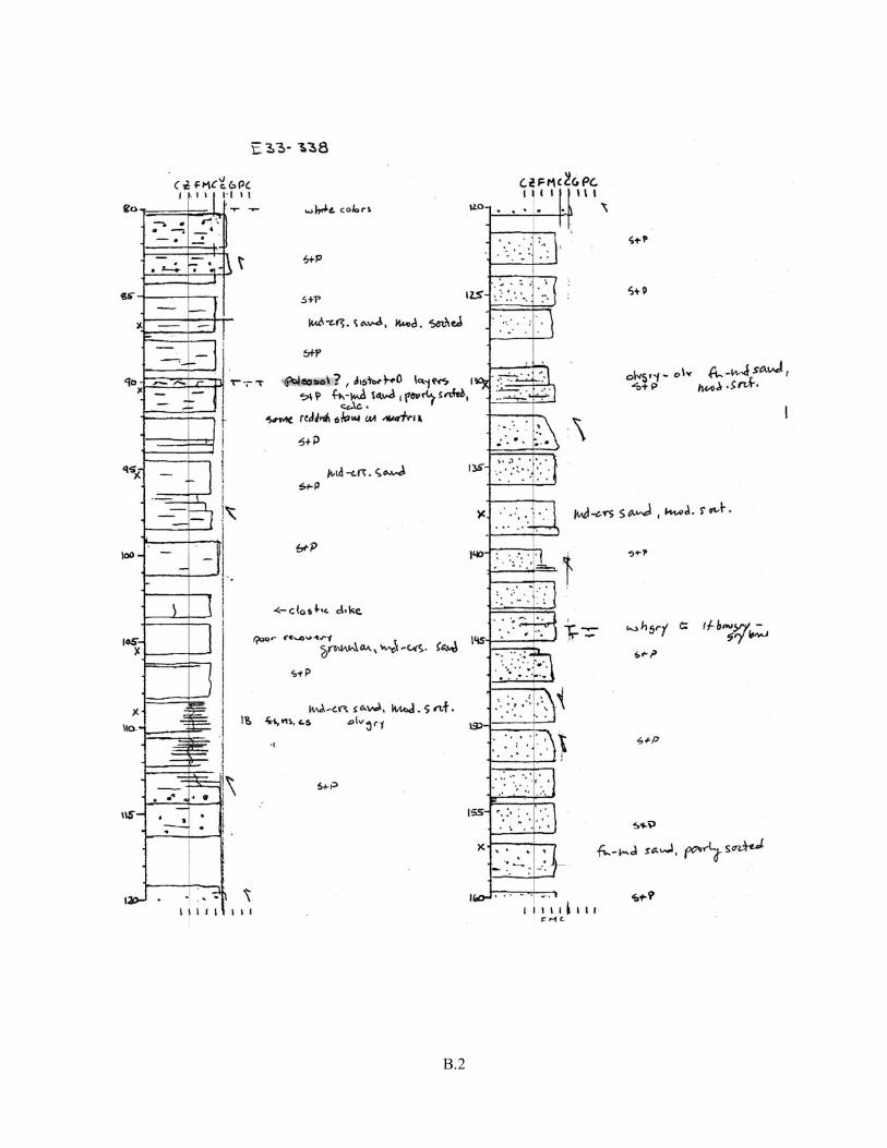
B.2

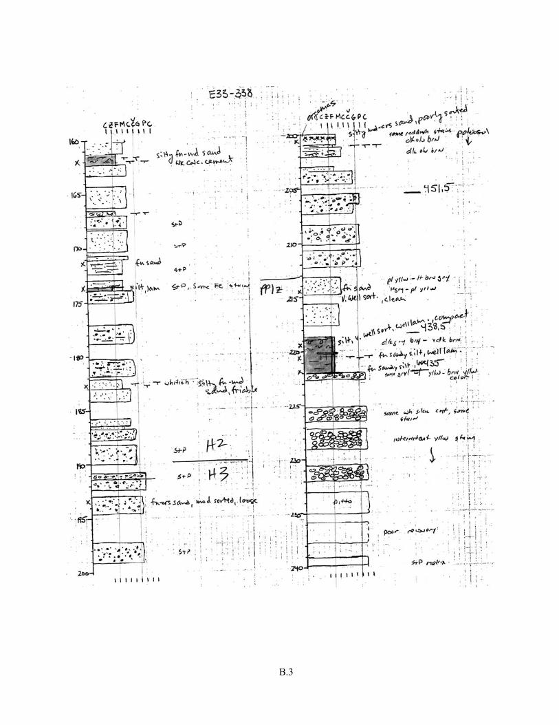
B.3

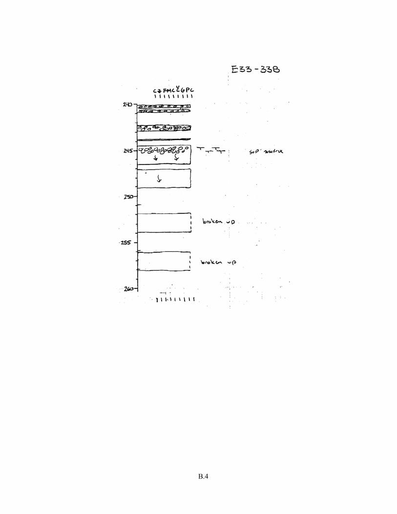
B.4

Appendix C

Summary of Geophysical Logs for Borehole 299-E33-338

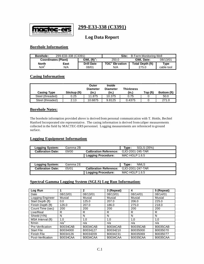
C.1 1

299-E33-338 (C3391)

Log Data Report Borehole Information:

Borehole : 299-E33-338 (C3391) Site: B Farm Monitoring Well Coordinates (Plant) GWL (ft)1: 250.0 GWL Date: 08/13/01

North East Drill Date TOC2 Elevation Total Depth (ft) Type N/A3 N/A 08/01 N/A 275.0 cable tool

Casing Information:

Casing Type Stickup (ft)

Outer Diameter

(in.)

Inside Diameter

(in.) Thickness

(in.) Top (ft) Bottom (ft) Steel (threaded) 0.25 11.875 10.375 0.75 0 50.0 Steel (threaded) 2.13 10.6875 9.8125 0.4375 0 271.0

Borehole Notes:

The borehole information provided above is derived from personal communication with T. Hottle, Bechtel Hanford Incorporated site representative. The casing information is derived from caliper measurements collected in the field by MACTEC-ERS personnel. Logging measurements are referenced to ground surface. Logging Equipment Information:

Logging System: Gamma 2B Type: SGLS (35%) Calibration Date: 09/00 Calibration Reference: GJO-2001-245-TAR

Logging Procedure: MAC-HGLP 1.6.5

Logging System: Gamma 2E Type: NMLS Calibration Date: 05/01 Calibration Reference: GJO-2001-247-TAR

Logging Procedure: MAC-HGLP 1.6.5

Spectral Gamma Logging System (SGLS) Log Run Information:

Log Run 1 2 3 (Repeat) 4 5 (Repeat) Date 08/13/01 08/13/01 08/13/01 08/14/01 08/14/01 Logging Engineer Musial Musial Musial Musial Musial Start Depth (ft) 0.0 125.0 207.0 206.0 225.0 Finish Depth (ft) 126.0 207.0 186.0 275.0 218.0 Count Time (sec) 200 200 200 200 200 Live/Real R R R R R Shield (Y/N) N N N N N MSA Interval (ft) 1.0 1.0 1.0 1.0 1.0 ft/min n/a4 n/a n/a n/a n/a Pre-Verification B0034CAB B0034CAB B0034CAB B0035CAB B0035CAB Start File B0034000 B0034127 B0034210 B0035000 B0035070 Finish File B0034126 B0034209 B0034231 B0035069 B0035077 Post-Verification B0034CAA B0034CAA B0034CAA B0035CAA B0035CAA

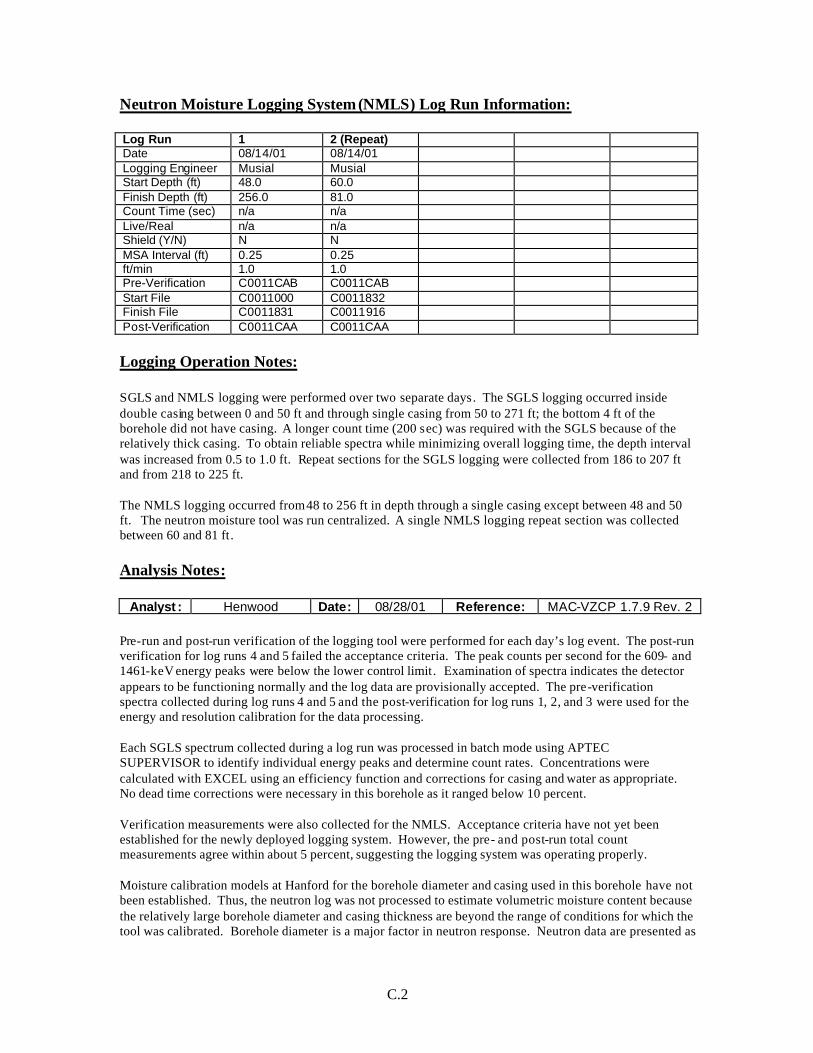
C.2

Neutron Moisture Logging System (NMLS) Log Run Information:

Log Run 1 2 (Repeat) Date 08/14/01 08/14/01 Logging Engineer Musial Musial Start Depth (ft) 48.0 60.0 Finish Depth (ft) 256.0 81.0 Count Time (sec) n/a n/a Live/Real n/a n/a Shield (Y/N) N N MSA Interval (ft) 0.25 0.25 ft/min 1.0 1.0 Pre-Verification C0011CAB C0011CAB Start File C0011000 C0011832 Finish File C0011831 C0011916 Post-Verification C0011CAA C0011CAA Logging Operation Notes: SGLS and NMLS logging were performed over two separate days. The SGLS logging occurred inside double casing between 0 and 50 ft and through single casing from 50 to 271 ft; the bottom 4 ft of the borehole did not have casing. A longer count time (200 sec) was required with the SGLS because of the relatively thick casing. To obtain reliable spectra while minimizing overall logging time, the depth interval was increased from 0.5 to 1.0 ft. Repeat sections for the SGLS logging were collected from 186 to 207 ft and from 218 to 225 ft. The NMLS logging occurred from 48 to 256 ft in depth through a single casing except between 48 and 50 ft. The neutron moisture tool was run centralized. A single NMLS logging repeat section was collected between 60 and 81 ft. Analysis Notes:

Analyst : Henwood Date: 08/28/01 Reference: MAC-VZCP 1.7.9 Rev. 2

Pre-run and post-run verification of the logging tool were performed for each day’s log event. The post-run verification for log runs 4 and 5 failed the acceptance criteria. The peak counts per second for the 609- and 1461-keV energy peaks were below the lower control limit. Examination of spectra indicates the detector appears to be functioning normally and the log data are provisionally accepted. The pre-verification spectra collected during log runs 4 and 5 and the post-verification for log runs 1, 2, and 3 were used for the energy and resolution calibration for the data processing. Each SGLS spectrum collected during a log run was processed in batch mode using APTEC SUPERVISOR to identify individual energy peaks and determine count rates. Concentrations were calculated with EXCEL using an efficiency function and corrections for casing and water as appropriate. No dead time corrections were necessary in this borehole as it ranged below 10 percent. Verification measurements were also collected for the NMLS. Acceptance criteria have not yet been established for the newly deployed logging system. However, the pre- and post-run total count measurements agree within about 5 percent, suggesting the logging system was operating properly. Moisture calibration models at Hanford for the borehole diameter and casing used in this borehole have not been established. Thus, the neutron log was not processed to estimate volumetric moisture content because the relatively large borehole diameter and casing thickness are beyond the range of conditions for which the tool was calibrated. Borehole diameter is a major factor in neutron response. Neutron data are presented as

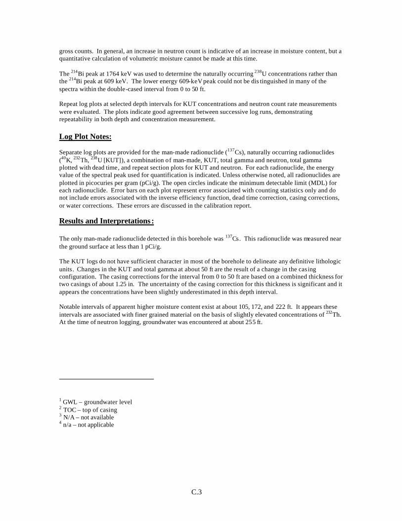
C.3

gross counts. In general, an increase in neutron count is indicative of an increase in moisture content, but a quantitative calculation of volumetric moisture cannot be made at this time. The 214Bi peak at 1764 keV was used to determine the naturally occurring 238U concentrations rather than the 214Bi peak at 609 keV. The lower energy 609-keV peak could not be dis tinguished in many of the spectra within the double-cased interval from 0 to 50 ft. Repeat log plots at selected depth intervals for KUT concentrations and neutron count rate measurements were evaluated. The plots indicate good agreement between successive log runs, demonstrating repeatability in both depth and concentration measurement. Log Plot Notes: Separate log plots are provided for the man-made radionuclide (137Cs), naturally occurring radionuclides (40K, 232Th, 238U [KUT]), a combination of man-made, KUT, total gamma and neutron, total gamma plotted with dead time, and repeat section plots for KUT and neutron. For each radionuclide, the energy value of the spectral peak used for quantification is indicated. Unless otherwise noted, all radionuclides are plotted in picocuries per gram (pCi/g). The open circles indicate the minimum detectable limit (MDL) for each radionuclide. Error bars on each plot represent error associated with counting statistics only and do not include errors associated with the inverse efficiency function, dead time correction, casing corrections, or water corrections. These errors are discussed in the calibration report.

Results and Interpretations : The only man-made radionuclide detected in this borehole was 137Cs. This radionuclide was measured near the ground surface at less than 1 pCi/g. The KUT logs do not have sufficient character in most of the borehole to delineate any definitive lithologic units. Changes in the KUT and total gamma at about 50 ft are the result of a change in the casing configuration. The casing corrections for the interval from 0 to 50 ft are based on a combined thickness for two casings of about 1.25 in. The uncertainty of the casing correction for this thickness is significant and it appears the concentrations have been slightly underestimated in this depth interval. Notable intervals of apparent higher moisture content exist at about 105, 172, and 222 ft. It appears these intervals are associated with finer grained material on the basis of slightly elevated concentrations of 232Th. At the time of neutron logging, groundwater was encountered at about 255 ft. 1 GWL – groundwater level 2 TOC – top of casing 3 N/A – not available 4 n/a – not applicable

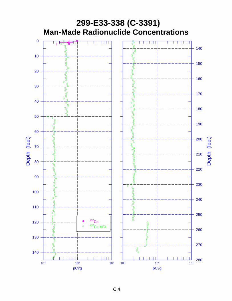
pCi/g10-1 100 101

Dep

th (

feet

)

140

150

160

170

180

190

200

210

220

230

240

250

260

270

280

pCi/g10-1 100 101

Dep

th (

feet

)

0

10

20

30

40

50

60

70

80

90

100

110

120

130

140

137Cs 137Cs MDL

Man-Made Radionuclide Concentrations299-E33-338 (C-3391)

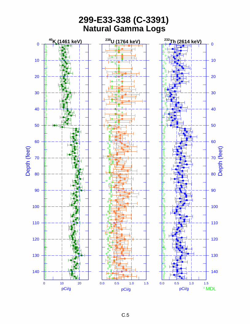
40K (1461 keV)

pCi/g0 10 20

Dep

th (

feet

)

0

10

20

30

40

50

60

70

80

90

100

110

120

130

140

238U (1764 keV)

pCi/g

0.0 0.5 1.0 1.5

232Th (2614 keV)

pCi/g0.0 0.5 1.0 1.5

Dep

th (

feet

)

0

10

20

30

40

50

60

70

80

90

100

110

120

130

140

Natural Gamma Logs

MDL

299-E33-338 (C-3391)

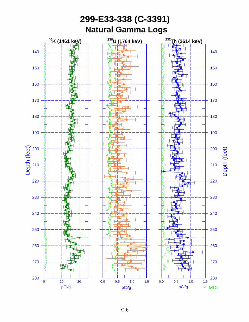
40K (1461 keV)

pCi/g0 10 20

Dep

th (

feet

)

140

150

160

170

180

190

200

210

220

230

240

250

260

270

280

238U (1764 keV)

pCi/g

0.0 0.5 1.0 1.5

232Th (2614 keV)

pCi/g0.0 0.5 1.0 1.5

Dep

th (

feet

)

140

150

160

170

180

190

200

210

220

230

240

250

260

270

280

Natural Gamma Logs

MDL

299-E33-338 (C-3391)

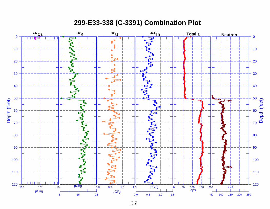
40K

pCi/g

5 15 25

137Cs

Dep

th (

feet

)

0

10

20

30

40

50

60

70

80

90

100

110

120

pCi/g10-1 100 101

238U

pCi/g0.0 0.5 1.0 1.5

232Th

pCi/g

0.0 0.5 1.0 1.5

Total γ

cps0 50 100 150 200

Neutron

cps

50 100 150 200 250

Dep

th (f

eet)

0

10

20

30

40

50

60

70

80

90

100

110

120

299-E33-338 (C-3391) Combination Plot

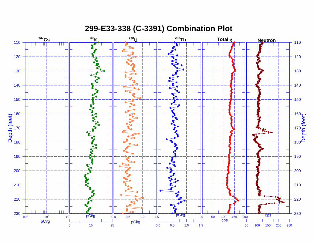
40K

pCi/g

5 15 25

137Cs

pCi/g10-1 100 101

Dep

th (

feet

)

110

120

130

140

150

160

170

180

190

200

210

220

230

238U

pCi/g0.0 0.5 1.0 1.5

232Th

pCi/g

0.0 0.5 1.0 1.5

Total γ

cps0 50 100 150 200

Neutron

cps

50 100 150 200 250

Dep

th (f

eet)

110

120

130

140

150

160

170

180

190

200

210

220

230

299-E33-338 (C-3391) Combination Plot

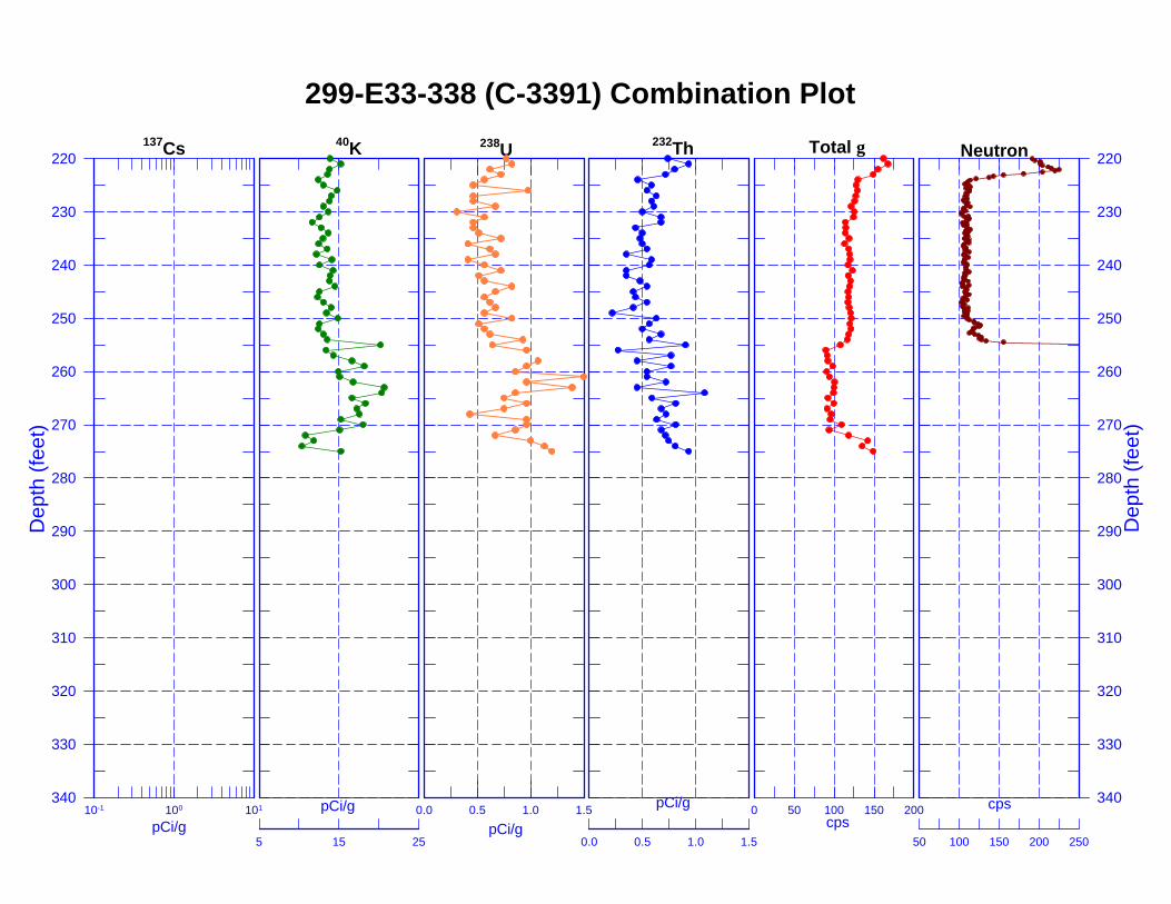
40K

pCi/g

5 15 25

137Cs

pCi/g10-1 100 101

Dep

th (

feet

)

220

230

240

250

260

270

280

290

300

310

320

330

340

238U

pCi/g0.0 0.5 1.0 1.5

232Th

pCi/g

0.0 0.5 1.0 1.5

Total γ

cps0 50 100 150 200

Neutron

cps

50 100 150 200 250

Dep

th (f

eet)

220

230

240

250

260

270

280

290

300

310

320

330

340

299-E33-338 (C-3391) Combination Plot

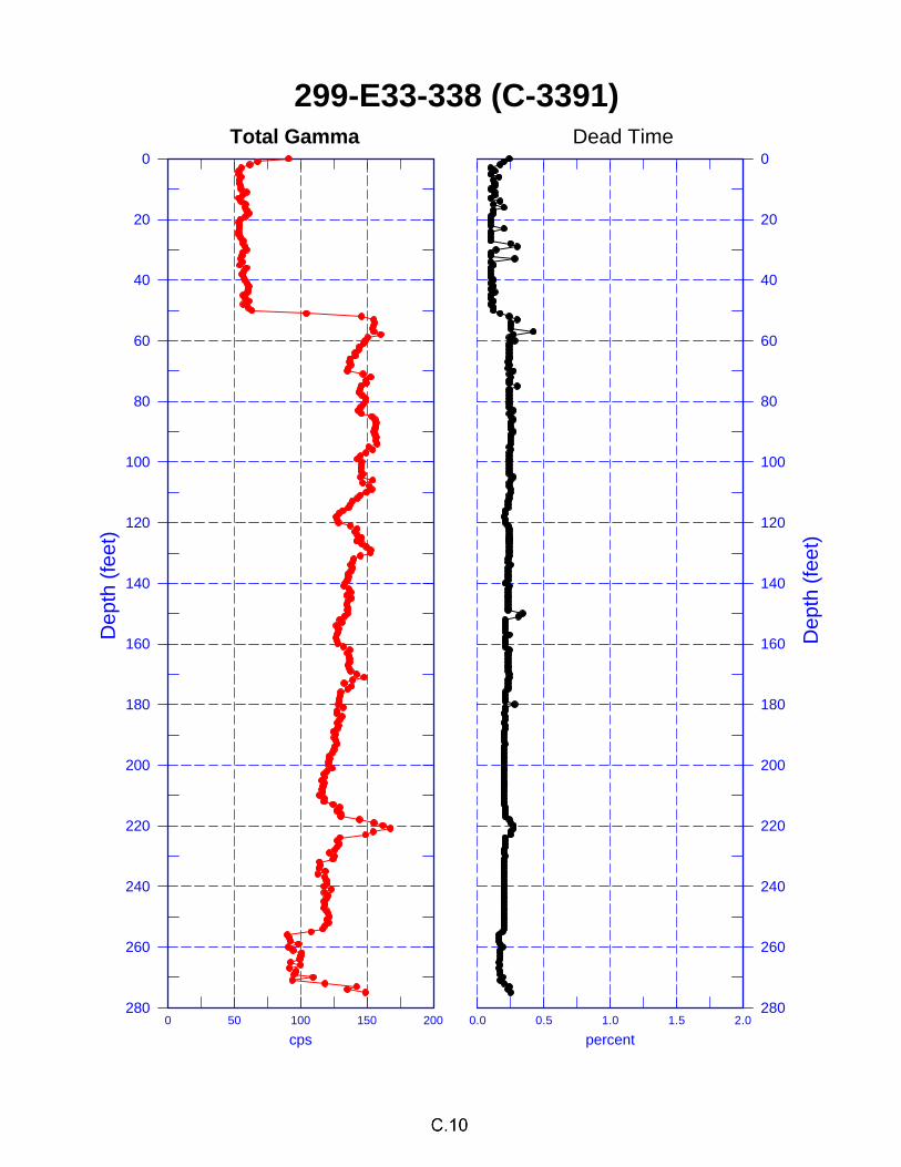
percent0.0 0.5 1.0 1.5 2.0

Dep

th (f

eet)

0

20

40

60

80

100

120

140

160

180

200

220

240

260

280

cps0 50 100 150 200

Dep

th (

feet

)

0

20

40

60

80

100

120

140

160

180

200

220

240

260

280

299-E33-338 (C-3391)Total Gamma Dead Time

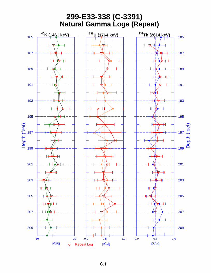
40K (1461 keV)

pCi/g10 20

Dep

th (

feet

)

185

187

189

191

193

195

197

199

201

203

205

207

209

238U (1764 keV)

pCi/g

0.0 0.5 1.0

232Th (2614 keV)

pCi/g0.0 0.5 1.0

Dep

th (

feet

)

185

187

189

191

193

195

197

199

201

203

205

207

209

Natural Gamma Logs (Repeat)299-E33-338 (C-3391)

Repeat Log

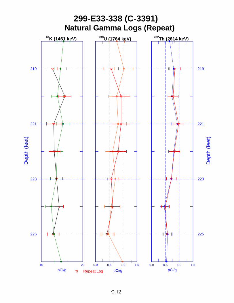
40K (1461 keV)

pCi/g10 20

Dep

th (

feet

)

219

221

223

225

238U (1764 keV)

pCi/g

0.0 0.5 1.0 1.5

232Th (2614 keV)

pCi/g0.0 0.5 1.0 1.5

Dep

th (

feet

)

219

221

223

225

Natural Gamma Logs (Repeat)299-E33-338 (C-3391)

Repeat Log

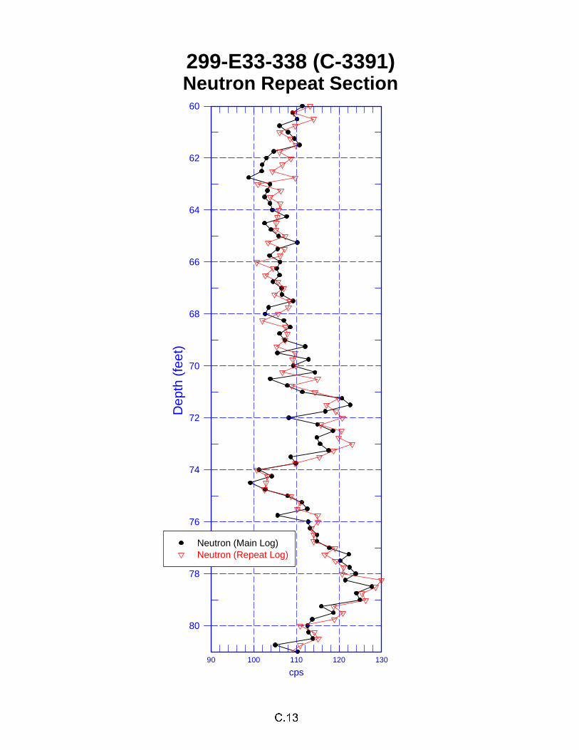
cps90 100 110 120 130

Dep

th (

feet

)

60

62

64

66

68

70

72

74

76

78

80

Neutron (Main Log)Neutron (Repeat Log)

Neutron Repeat Section299-E33-338 (C-3391)

PNNL-14121

Distr.1

Distribution No. of Copies OFFSITE

Dr. Harry Babad 2540 Cordoba Court Richland, WA 99352-1609 Pat Brady Geochemistry Department, 6118 Sandia National Laboratories P.O. Box 5800 Albuquerque, New Mexico 87185-0750 Charles R. Bryan Sandia National Laboratories 4100 National Parks Highway Carlsbad, N.M. 88220 Susan Carroll Lawrence Livermore National Laboratory Mail Stop L-219 Livermore, CA 94550 Jon Chorover Associate Professor - Environmental

Chemistry Department of Soil, Water and

Environmental Science Shantz 429, Building #38 University of Arizona Tucson, AZ 85721-0038 Dave G. Coles Coles Environmental Consulting 750 South Rosemont Rd West Linn, OR 97068

No. of Copies

Mark Conrad Department of Earth and Planetary Sciences University of California Berkeley Berkeley, CA 94720 Dr. James A. Davis U.S. Geological Survey MS-465 345 Middlefield Rd. Menlo Park, CA 94025 Donald J. DePaolo Geology & Geophysics Dept., MC4767 University of California Berkeley, CA 94720-4767 Dirk A. Dunning Oregon Office of Energy 625 Mariona St. N. E. Salem, OR 97301-3742 Mark Ewanic MSE Technology Applications, Inc. 200 Technology Way Butte, MT 59701 Markus Flury Department of Crop and Soil Sciences Washington State University Pullman, WA 99164 Amy P. Gamerdinger 2122 E. Hawthorne Tucson, AZ 85719

PNNL-14121

Distr.2

No. of Copies

Jim Harsh Department of Crop & Soil Sciences Washington State University Johnson Hall – Room 249 Pullman WA 99164-6420 Dr. Cliff Johnston Soil Chemistry and Mineralogy 1150 Lily Hall Purdue University West Lafayette, IN 47907-1150 Dr. Daniel I. Kaplan Westinghouse Savannah River Company Bldg. 774-43A, Rm 215 Aiken, SC 29808 Dr. Peter C. Lichtner Los Alamos National Laboratory P.O. Box 1663 Los Alamos, NM 87545 Patrick Longmire Los Alamos National Laboratory Mail Stop J534 P.O. Box 1663 Los Alamos, NM 87545 Kate Maher The Center for Isotope Geochemistry 301 McCone Hall University of California, Berkeley Berkeley, CA 94702-4746 Melanie A. Mayes Environmental Sciences Division Oak Ridge National Laboratory P.O. Box 2008 Oak Ridge,TN 37831-6038

No. of Copies

Dr. Kathryn L. Nagy Department of Earth and Environmental

Sciences University of Illinois at Chicago (MC-186) 845 West Taylor Street Chicago, IL 60607-7059 Heino Nitsche Director, Center for Advanced Environmental

and Nuclear Studies Lawrence Berkeley National Laboratory 1 Cyclotron Road MS 70A-1150 Berkeley, CA 94720 Phil Reed U.S. Nuclear Regulatory Commission Office of Nuclear Regulatory Research Division of Systems Analysis and Regulatory

Effectiveness Radiation Protection, Env. Risk and Waste

Management Branch Mail Stop: T9-F31 Washington, DC 20555-0001 Richard J. Reeder Dept. of Geosciences State University of New York at Stony Brook Stony Brook, NY 11794-2100 Al Robinson 68705, E 715 PRNE Richland WA 99352 Phil Rogers 13 Mountain Oak Littleton, CO 80127

PNNL-14121

Distr.3

No. of Copies

David Shafer Desert Research Institute University of Nevada P.O. Box 19040 Las Vegas, NV 89132-0040 Dawn A. Shaughnessy Glenn T. Seaborg Center Lawrence Berkeley National Laboratory 1 Cyclotron Road MS 70A-1150 Berkeley, CA 94720 Doug Sherwood Rivers Edge Environmental 1616 Riverside Drive West Richland, WA 99353 David K. Shuh Lawrence Berkeley National Lab 1 Cyclotron Road Mail Stop 70A-1150 Berkeley, CA 94720 James "Buck" Sisson Idaho National Engineering and

Environmental Laboratory PO Box 1625, MS-2107 Idaho Falls, ID 83415-2107 Carl I. Steefel Lawrence Livermore National Laboratory Earth & Environmental Sciences Directorate Mail Stop L-204 PO Box 808 Livermore, CA 94551-9900 Dr. Samuel J. Traina, Director Sierra Nevada Research Institute University of California, Merced P.O. Box 2039 Merced, CA 95344

No. of Copies

Dr. T. T. Chuck Vandergraaf Atomic Energy Of Canada, Limited Whiteshell Nuclear Research Establishment Pinawa, Manitoba ROE 1LO Canada Dr. Jiamin Wan Lawrence Berkeley National Laboratory 1 Cyclotron Rd. MS 70-0127A Berkeley, CA 94720 Mr. Ronald G. Wilhelm Office of Radiation and Indoor Air 401 M Street, S.W. Mail Code 6603J Washington, D.C. 20460 W. Alexander Williams US Department of Energy Office of Environmental Restoration EM-33 19901 Germantown Road Germantown, MD 20874-1290

ONSITE 4 DOE Office of River Protection C. A. Babel H6-60 P. E. LaMont H6-60 R. W. Lober H6-60 R. B. Yasek H6-60 8 DOE Richland Operations Office B. L. Foley A6-38 J. P. Hanson A5-13 R. D. Hildebrand A6-38 K. A. Kapsi A5-13 J. G. Morse A6-38 K. M. Thompson A6-38 DOE Public Reading Room (2) H2-53

PNNL-14121

Distr.4

No. of Copies Bechtel Hanford, Inc. K. R. Fecht H0-02 18 CH2M Hill Hanford Group, Inc. J. E. Auten E6-35 K. C. Burgard L6-57 M. P. Connelly E6-35 E. A. Fredenburg H9-03 T. E. Jones (2) E6-35 A. J. Knepp (2) H6-60 F. M. Mann (5) E6-35 W. J. McMahon E6-35 C. W. Miller H9-03 D. A. Myers (3) E6-35 3 Duratek Federal Services, Inc., Northwest Operations M. G. Gardner H1-11 K. D. Reynolds H1-11 D. E. Skoglie H1-11 3 Environmental Protection Agency Nick Ceto B5-01 D. A. Faulk B5-01 M. L. Goldstein B5-01 2 Flour Federal Services R. Khaleel E6-17 R. J. Puigh E6-17 5 Flour Hanford, Inc. T. W. Fogwell E6-35 B. H. Ford E6-35 J. G. Hogan H1-11 V. G. Johnson E6-35 M. I. Wood H8-44 64 Pacific Northwest National Laboratory S. R. Baum P7-22 B. N. Bjornstad (3) K6-81 C. F. Brown P7-22

No. of Copies R. W. Bryce E6-35 R. E. Clayton P7-22 W. J. Deutsch K6-81 P. E. Dresel K6-96 K. M. Geisler P7-22 M. J. Fayer K9-33 A. R. Felmy K8-96 M. D. Freshley K9-33 J. S. Fruchter K6-96 D. G. Horton K6-81 J. P. Icenhower K6-81 C. T. Kincaid E6-35 K. M. Krupka K6-81 I. V. Kutnyakov P7-22 G. V. Last (3) K6-81 V. L. LeGore P7-22 M. J. Lindberg P7-22 C. W. Lindenmeier (2) P7-22 W. J. Martin K6-81 S. V. Mattigod K6-81 B. P. McGrail K6-81 P. D. Meyer BPO C. J. Murray K6-81 S. M. Narbutovskih K6-96 R. D. Orr K6-81 E. M. Pierce K6-81 S. P. Reidel K6-81 R. J. Serne (20) P7-22 H. T. Schaef K6-81 W. Um P7-22 M. Valenta P7-22 T. S. Vickerman P7-22 B. A. Williams K6-81 S. B. Yabusaki K9-36 J. M. Zachara K8-96 Hanford Technical Library (2) P8-55