Geochemical Modeling of CO2 Sequestration in Dolomitic

University of South FloridaScholar Commons

Graduate Theses and Dissertations Graduate School

10-25-2010

Geochemical Modeling of CO2 Sequestration inDolomitic Limestone AquifersMark W. ThomasUniversity of South Florida

Follow this and additional works at: http://scholarcommons.usf.edu/etd

Part of the American Studies Commons

This Thesis is brought to you for free and open access by the Graduate School at Scholar Commons. It has been accepted for inclusion in GraduateTheses and Dissertations by an authorized administrator of Scholar Commons. For more information, please contact [email protected].

Scholar Commons CitationThomas, Mark W., "Geochemical Modeling of CO2 Sequestration in Dolomitic Limestone Aquifers" (2010). Graduate Theses andDissertations.http://scholarcommons.usf.edu/etd/3708

http://scholarcommons.usf.edu/?utm_source=scholarcommons.usf.edu%2Fetd%2F3708&utm_medium=PDF&utm_campaign=PDFCoverPages

http://scholarcommons.usf.edu/?utm_source=scholarcommons.usf.edu%2Fetd%2F3708&utm_medium=PDF&utm_campaign=PDFCoverPages

http://scholarcommons.usf.edu?utm_source=scholarcommons.usf.edu%2Fetd%2F3708&utm_medium=PDF&utm_campaign=PDFCoverPages

http://scholarcommons.usf.edu/etd?utm_source=scholarcommons.usf.edu%2Fetd%2F3708&utm_medium=PDF&utm_campaign=PDFCoverPages

http://scholarcommons.usf.edu/grad?utm_source=scholarcommons.usf.edu%2Fetd%2F3708&utm_medium=PDF&utm_campaign=PDFCoverPages

http://scholarcommons.usf.edu/etd?utm_source=scholarcommons.usf.edu%2Fetd%2F3708&utm_medium=PDF&utm_campaign=PDFCoverPages

http://network.bepress.com/hgg/discipline/439?utm_source=scholarcommons.usf.edu%2Fetd%2F3708&utm_medium=PDF&utm_campaign=PDFCoverPages

mailto:[email protected]

Geochemical Modeling of CO2 Sequestration

in Dolomitic Limestone Aquifers

by

Mark W. Thomas

A thesis submitted in partial fulfillment

of the requirements for the degree of

Master of Science in Environmental Engineering

Department of Civil and Environmental Engineering

College of Engineering

University of South Florida

Major Professor: Jeffrey Cunningham, Ph.D.

Mark Stewart, Ph.D.

Maya Trotz, Ph.D.

Date of Approval:

October 25, 2010

Keywords: carbon capture and storage, activity coefficient, CO2 solubility model,

mineral precipitation and dissolution, geochemistry, non-linear

Copyright © 2010, Mark W. Thomas

Acknowledgements

The research leading to this thesis was funded by the State of Florida through the

Florida Energy Systems Consortium (FESC). Any opinions, findings, conclusions, or

recommendations are those of the author and do not necessarily reflect the views of

FESC.

I would like to thank Dr. Jeffrey Cunningham at the University of South Florida for

giving me the opportunity to join his research team and become part of this project, and

for the constructive comments, mentoring, and advice given during the writing of this

thesis. I would also like to thank the faculty of the Department of Civil and

Environmental Engineering at the University of South Florida for their teaching efforts,

and to all those who encouraged me during the preparation of this thesis.

i

Table of Contents

List of Tables ..................................................................................................................... iii

List of Figures .................................................................................................................... iv

Abstract .............................................................................................................................. vi

1: Introduction ................................................................................................................ 1

2: Literature Review....................................................................................................... 5

3: Estimating Thermodynamic Variables ...................................................................... 9

3.1: Equilibrium Constant, K ............................................................................... 9

3.2: Activity Coefficient, γ ................................................................................. 10

3.2.1: Activity Coefficient for Neutral Aqueous Species ....................................11

3.2.2: Activity Coefficient for Charged Aqueous Species ...................................11

3.2.3: Activity Coefficient for Aqueous CO2 .......................................................17

3.2.3.1:Method of Drummond (22)..................................................................18

3.2.3.2:Method of Rumpf et al. (23) ................................................................18

3.2.3.3:Method of Duan and Sun (25) .............................................................19

3.3: Estimating the Fugacity Coefficient for Gaseous and Supercritical

CO2, φCO2 .................................................................................................... 20

3.3.1: Method of Spycher and Reed (26) .............................................................20

3.3.2: Method of Duan et al. (20) .........................................................................21

3.4: Estimating the Activity of Water, aW .......................................................... 21

3.5: Aqueous CO2 Concentration, mCO2 ............................................................. 23

3.5.1: Equilibrium Constant .................................................................................23

3.5.2: Method of Duan and Sun (25) ...................................................................24

3.5.3: Method of Spycher and Pruess (21) ...........................................................25

3.5.4: Spycher and Pruess (21) adaptation of the method of

Duan and Sun (25) .....................................................................................27

3.6: Summary ..................................................................................................... 29

4: Model Development................................................................................................. 30

ii

4.1: Model Overview ......................................................................................... 30

4.2: System of Geochemical Equations ............................................................. 30

4.2.1: Rock Minerals ............................................................................................31

4.2.2: Carbonate System ......................................................................................32

4.2.3: Aqueous Complexes ..................................................................................33

4.2.4: Salinity .......................................................................................................34

4.2.5: Water (H2O) System ..................................................................................35

4.2.6: Charge Balance ..........................................................................................36

4.3: Iterative Solution Procedure ....................................................................... 36

4.3.1: Inner Iteration Loop ...................................................................................37

4.3.2: Outer Iteration Loop ..................................................................................40

4.4: Model Implementation ................................................................................ 41

4.5: Model Limitations ....................................................................................... 42

4.6: Model Outputs ............................................................................................ 42

4.7: Comparison of Thermodynamic Sub-models ............................................. 43

5: Model Results .......................................................................................................... 50

5.1: Effect of Initial pH ...................................................................................... 50

5.2: Effect of CO2 Injection Pressure ................................................................. 54

5.3: Effect of Salinity ......................................................................................... 58

5.4: Effect of Temperature ................................................................................. 62

5.5: Effects on Porosity, ε .................................................................................. 65

5.6: Choice of Thermodynamic Sub-model for CO2 Parameter

Estimation ................................................................................................... 69

6: Summary and Conclusion ........................................................................................ 70

Works Cited ...................................................................................................................... 71

iii

List of Tables

Table 1: Equilibrium Reactions for Mineral Dissolution and Precipitation .....................31

Table 2: Equilibrium Reactions for Carbonate Species ....................................................32

Table 3: Equilibrium Reactions for Aqueous Complexes.................................................33

Table 4: Equilibrium Reactions for H2O Dissociation ......................................................35

Table 5: Combinations of Sub-Models for CO2 Thermodynamic

Parameter Estimation ..........................................................................................44

Table 6: Brine Densities at Various Salinities and Temperatures.....................................66

Table 7: Mineral Densities ................................................................................................67

Table 8: Porosity and Residual Brine Saturation Scenarios..............................................67

Table 9: Change in Porosity for Scenarios 1-3 Using Various Combinations of

Initial pH, CO2 Injection Pressure, Salinity, Temperature..................................68

iv

List of Figures

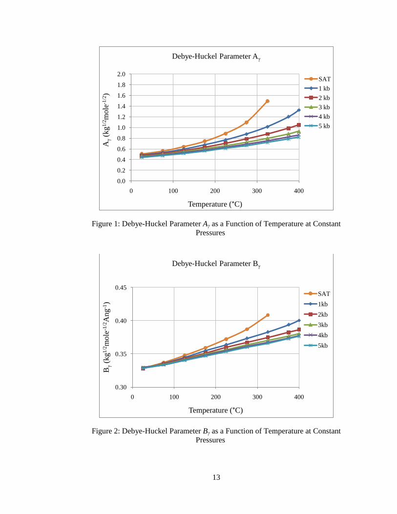
Figure 1: Debye-Huckel Parameter Aγ as a Function of Temperature at

Constant Pressures ...........................................................................................13

Figure 2: Debye-Huckel Parameter Bγ as a Function of Temperature at


Figure 3: Helgeson Interaction Parameter bNaCl as a Function of Temperature at


Figure 4: Helgeson Interaction Parameter bNa+,Cl- as a Function of Temperature

at Constant Pressures .......................................................................................17

Figure 5: Inner Iteration Loop for Pre-CO2 Injection ......................................................37

Figure 6: Inner Iteration Loop for Post-CO2 Injection ....................................................38

Figure 7: Outer Iteration Loop ........................................................................................41

Figure 8: Equilibrium pH for Various Choices of Thermodynamic Sub-Models ...........45

Figure 9: CO2 Molality for Various Choices of Thermodynamic Sub-Models ..............45

Figure 10: Calcite Dissolution for Various Choices of Thermodynamic

Sub-Models ......................................................................................................46

Figure 11: Dolomite Dissolution for Various Choices of Thermodynamic

Sub-Models ......................................................................................................46

Figure 12: Gypsum Precipitation for Various Choices of Thermodynamic

Sub-Models ......................................................................................................47

Figure 13: Net CO2 Storage for Various Choices of Thermodynamic Sub-models .........47

Figure 14: Equilibrium pH as a Function of Initial pH .....................................................51

Figure 15: Calcite Dissolution as a Function of Initial pH ................................................51

Figure 16: Dolomite Dissolution as a Function of Initial pH ............................................52

Figure 17: Gypsum Precipitation as a Function of Initial pH ...........................................52

v

Figure 18: Net CO2 Storage as a Function of Initial pH ....................................................53

Figure 19: Equilibrium pH as a Function of CO2 Injection Pressure ................................54

Figure 20: Calcite Dissolution as a Function of CO2 Injection Pressure ..........................55

Figure 21: Dolomite Dissolution as a Function of CO2 Injection Pressure .......................55

Figure 22: Gypsum Precipitation as a Function of CO2 Injection Pressure ......................56

Figure 23: Net CO2 Storage as a Function of CO2 Injection Pressure ..............................56

Figure 24: Equilibrium pH as a Function of Salinity ........................................................58

Figure 25: Calcite Dissolution as a Function of Salinity ...................................................59

Figure 26: Dolomite Dissolution as a Function of Salinity ...............................................59

Figure 27: Gypsum Precipitation as a Function of Salinity ..............................................60

Figure 28: Net CO2 Storage as a Function of Salinity .......................................................60

Figure 29: Equilibrium pH as a Function of Temperature ................................................62

Figure 30: Calcite Dissolution as a Function of Temperature ...........................................63

Figure 31: Dolomite Dissolution as a Function of Temperature .......................................63

Figure 32: Gypsum Precipitation as a Function of Temperature .......................................64

Figure 33: Net CO2 Storage as a Function of Temperature ...............................................64

vi

Abstract

Geologic sequestration of carbon dioxide (CO2) in a deep, saline aquifer is being

proposed for a power-generating facility in Florida as a method to mitigate contribution

to global climate change from greenhouse gas (GHG) emissions. The proposed repository

is a brine-saturated, dolomitic-limestone aquifer with anhydrite inclusions contained

within the Cedar Keys/Lawson formations of Central Florida. Thermodynamic modeling

is used to investigate the geochemical equilibrium reactions for the minerals calcite,

dolomite, and gypsum with 28 aqueous species for the purpose of determining the

sensitivity of mineral precipitation and dissolution to the temperature and pressure of the

aquifer and the salinity and initial pH of the brine. The use of different theories for

estimating CO2 fugacity, solubility in brine, and chemical activity is demonstrated to

have insignificant effects on the predicted results. Nine different combinations of

thermodynamic models predict that the geochemical response to CO2 injection is calcite

and dolomite dissolution and gypsum precipitation, with good agreement among the

quantities estimated. In all cases, CO2 storage through solubility trapping is demonstrated

to be a likely process, while storage through mineral trapping is predicted to not occur.

Over the range of values examined, it is found that net mineral dissolution and

precipitation is relatively sensitive to temperature and salinity, insensitive to CO2

injection pressure and initial pH, and significant changes to porosity will not occur.

1

1: Introduction

It is becoming increasingly accepted by the scientific community that global climate

change due to anthropogenic emissions of greenhouse gases (GHG) is occurring.

Greenhouse gases are being released at higher rate than the biosphere’s ability to absorb

them, with a resulting net increase of GHG concentrations in the atmosphere (1). A

greenhouse gas of primary concern is carbon dioxide (CO2). One of the major sources of

CO2 emissions is the combustion of fossil fuels for power generation and industrial

processes in today’s energy-intensive global economy (1). Part of the long-term solution

to global climate change is widespread adoption of low carbon fuels for power generation

and industrial processes; however, in the near term, techniques to reduce CO2 emissions

are being investigated (1).

One of the more promising mitigation techniques being investigated is capturing CO2

from large point-source emitters and storing it to prevent release to the atmosphere (1; 2).

This process, commonly referred to as carbon capture and storage (CCS), relies on

technologies that have already been implemented at smaller scales by the oil and gas

industries for enhanced oil recovery (EOR) and CO2 disposal from natural gas refining

(1; 2). Proposed repositories for large-scale storage of captured CO2 include depleted oil

and natural gas fields, coal beds, the deep ocean, and deep saline aquifers (1; 2). Deep

saline aquifers are ideal candidates for storing CO2 because they are commonly

2

found throughout the world, often have large storage capacity and ideal geologic

properties, are not used as drinking water sources, and are isolated from the biosphere (1;

3; 4).

Injection of CO2 into deep aquifers for geologic storage requires a compressed CO2

stream recovered from industrial processes and an injection well drilled into the receiving

formation (2). Typically, the CO2 is injected into and maintained within the aquifer under

supercritical conditions to take advantage of higher density of the CO2 phase under these

conditions; in other words, more mass of CO2 is stored per bulk aquifer volume when it is

supercritical versus when it is gaseous (1). As CO2 injection into the aquifer continues, it

will displace the native brine as it sweeps through the formation (2). As the native brine

is being displaced by CO2 sweeping, some brine will remain trapped in pores due to

capillary forces. This trapped brine is known as the residual brine saturation, and may

absorb CO2 from the injected CO2 phase.

Carbon dioxide storage in deep saline aquifers involves many uncertainties from

geochemical and geologic perspectives. Carbon dioxide storage in a deep saline aquifer

results in numerous geochemical reactions between the native brine and the rock minerals

that comprise the aquifer formation (2; 4). These reactions are expected to result in

dissolution and precipitation of different minerals, and this can have consequences related

to formation integrity and storage efficiency (4). Excess mineral dissolution could

weaken the aquifer formation, which could increase the risk of CO2 escaping into other

geologic formations (1; 5). Conversely, excess mineral precipitation could decrease the

porosity of the formation, potentially decreasing the permeability of the aquifer to

injected CO2 or decreasing the available volume for bulk CO2 storage (6).

3

The University of South Florida has been investigating the feasibility of capturing

CO2 from a power generating facility in Polk County, Florida and storing it in a deep,

dolomitic-limestone aquifer located within the Cedar Keys/Lawson formation of Central

Florida (7; 8; 9). Geochemical modeling of CCS in this formation has been previously

performed by researchers at the University of South Florida using TOUGHREACT

software (7). The previous models predicted that CO2 injection in this formation would

lower the pH of the native brine, resulting in the dissolution of calcite and dolomite and

the precipitation of gypsum (7). Additionally, it was found that porosity increased very

slightly due to excess mineral dissolution in areas where CO2-saturated brine interacts

with the mineral phase (7). However, further investigation into the methods used by the

TOUGHREACT software for estimating thermodynamic parameters (activity

coefficients, fugacity coefficients, solubility) is deemed warranted. Alternative

geochemical models of CCS in the Cedar Keys/Lawson injection zone that yield similar

predictions to those of TOUGHREACT simulations would lend support to the results

reported by Cunningham et al. (7).

The first objective of this thesis is to develop a general thermodynamic framework for

geochemical modeling of CO2 injection into a dolomitic limestone aquifer that is

representative of the Cedar Keys/Lawson injection zone. After developing a framework

for geochemical modeling, the next objective is to examine the system sensitivity to

different methods for estimating thermodynamic parameters for CO2. The third objective

is to investigate the system sensitivity to geophysical and chemical parameters like initial

pH, CO2 injection pressure, brine salinity, and temperature. The final objective of this

4

thesis is to use the results of the geochemical model to estimate changes in porosity

induced by CO2 injection.

This thesis will first discuss existing knowledge of CO2 injection into deep saline

aquifers (Chapter 2). It will then explore the thermodynamic variables involved in

describing the geochemical system and different methods for their estimation (Chapter 3).

This will be followed by discussion of the calculation methodology required to solve

non-linear geochemical equations that describe the chemistry induced by CO2 dissolution

into residual brine (Chapter 4). Finally, data obtained from the models related to mineral

precipitation and dissolution and changes in porosity will be presented (Chapter 5), and

appropriate conclusions will be drawn (Chapter 6).

5

2: Literature Review

A great deal of research on CO2 injection into geologic formations is available in the

literature for a wide variety of conditions and intended purpose of storage. While the idea

of widespread and large-scale capture and storage of CO2 from facilities like fossil fuel

power plants is relatively new, the process and technologies of injecting CO2

underground are not (1; 10). Carbon dioxide injection has been used primarily in the oil

industry as a way to increase oil production from declining fields and in the gas industry

as a way to dispose of CO2 that is stripped from natural gas during refining operations,

though at a smaller scale than would be needed for widespread adoption of CO2

sequestration from power generation facilities (1; 10). Much of the research has focused

on CO2 storage in sandstone formations because they often hold oil or natural gas and

often include the possibility of mineral trapping due to the presence of aluminosilicate

minerals (1; 11; 12). However, recent research has also considered the possibility of

using carbonate formations as CO2 storage repositories (5; 6; 13). Studies have included

both laboratory experiments and computer modeling of expected conditions for a CO2

injection process into a carbonate aquifer (4; 5; 6; 13; 14).

Carbon dioxide is trapped in a deep saline aquifer by several processes. Initially, CO2

is trapped within the pores of the aquifer formation due to capillary forces and underneath

the aquifer confining layer by hydrodynamic forces due to buoyancy (1; 2). As time

passes, CO2 is further trapped in the aquifer by dissolution and speciation into

6

native brine through solubility and ionic trapping (1; 2). Finally, dissolved carbonate

species can be further trapped by combining with dissolved cations to form solid mineral

precipitates in thermodynamic equilibrium with the brine during a process known as

mineral trapping (1; 2).

It has been suggested that mineral trapping of CO2 in a typical calcium carbonate

aquifer (i.e. calcium or calcite is present in significant amounts) is not a viable

mechanism for CO2 storage due to the increase in solubility of calcium carbonate

minerals at low pH conditions resulting from CO2 dissolution into native brine (4; 6; 13).

This is in contrast to the precipitation of low-solubility carbonate minerals that is

expected in aluminosilicate-rich, iron-rich, or magnesium-rich aquifer formations (3; 10;

11). Modeling performed by others typically predicts a pH around 4.8 as a result of CO2

dissolution into brine contained within a carbonate aquifer (5; 7). Solution buffering by

bicarbonate ion (HCO3-) due to dissolution of carbonate-containing minerals is predicted

to be the dominant mechanism for determining the pH of CO2-saturated brine in

carbonate aquifers (4; 5; 7). Additionally, solution buffering enhances the dissolution of

CO2, and this can contribute to additional CO2 storage by solubility trapping (5; 15).

Calcite, if present, is always predicted to dissolve locally when it is in contact with CO2-

saturated brine (5; 6; 7; 13), although some studies have found that it can precipitate

downstream from areas of high dissolution due to particle trapping in pores and exposure

to high bicarbonate concentration in displaced brine (6). The net calcite dissolution is

predicted to be relatively low when compared to its abundance in the mineral phase (i.e.,

aquifer matrix) (5; 7). However, near the injection well, some have noted that calcite

dissolution can be quite high, leading to large increases in porosity with high connectivity

7

– i.e. channeling through the rock formation (4). Dolomite, if it is also present in the

mineral phase, has been predicted by some models to dissolve along with calcite when in

contact with CO2 saturated brine (5; 7). However, other models predict that dolomite can

precipitate when magnesium-saturated brine encounters a pure calcite phase (13).

Cunningham et al. also suggest that gypsum precipitates due to increased Ca2+

concentrations released by calcite and dolomite dissolution when sulfate ion (SO42-

) is

present (7).

In the literature, most computer models of single-phase CO2 injection into carbonate

aquifers typically predict that that permeability and porosity are not likely to be

significantly affected (5; 7; 13). However, some research suggests that micro-scale

anisotropic features of the aquifer formation can influence mineral dissolution and

precipitation and have a significant effect on changes in porosity and permeability (13;

14). This is consistent with lab experiments performed by Izgec et al. (6). Others have

explored the difference between injecting pure-phase CO2 versus CO2-saturated brine and

found that injection of CO2-saturated brine can damage the aquifer formation by

excessive carbonate mineral dissolution. This is a result of continuous refreshing of CO2-

saturated brine that is cation-deficient near the wellhead (4). In general, however, most

studies do not predict that changes in porosity and permeability due to geochemical

effects of CO2 injection into carbonate aquifers represent a significant impediment to

implementation (4; 5; 7).

Most research into the geochemical effects of CO2 injection into a carbonate aquifer

suggests that carbonate minerals will dissolve. However, there is some disagreement over

the extent of carbonate mineral dissolution and the effects of this dissolution on porosity

8

and permeability. Furthermore, there is a lack of data comparing the effects of the choices

of different methods for estimating thermodynamic parameters on the geochemical

system. Finally, there is little information available in the literature on the sensitivity of

the geochemistry involved with CO2 injection into a carbonate aquifer to physical and

chemical parameters like initial pH, CO2 injection pressure, and brine salinity.

9

3: Estimating Thermodynamic Variables

To model the effects of CO2 injection into a carbonate aquifer, the system must be

described in a thermodynamic context. This thermodynamic description is based on

solubility equilibrium relationships for minerals, aqueous complexes, and CO2 with ions

dissolved in the native brine of the aquifer formation. Deviations from ideal

thermodynamic behavior due to high pressure, salinity, and temperature are accounted for

by activity coefficients for aqueous species and by a fugacity coefficient for the

supercritical CO2 phase.

3.1: Equilibrium Constant, K

The equilibrium constant, K, represents the ratio of product activities to reactant

activities that occurs when the forward and reverse rates of a reaction are equal (i.e., the

reaction is at equilibrium). Consider a chemical reaction where the reactants A and B are

in equilibrium with the products C and D. The reaction can be written in the following

manner:

Equation 1

where lowercase letters represent a stoichiometric coefficient and uppercase letters

represent a chemical species. The equilibrium constant is given by the following

expression:

10

Equation 2

where aj represents the chemical activity of species j.

Equilibrium constants for many reactions have been determined experimentally and

values are available in the literature. For this study, equilibrium constants are taken from

the thermodynamic database included with the TOUGHREACT geochemical modeling

software (16). This database has equilibrium constants for many geochemical reactions as

functions of temperature and is considered valid over a temperature range of 0-300°C

(16). The equilibrium constants for most reactions considered in this paper are calculated

using an equation of the following form (16):

Equation 3

where K is the equilibrium constant, T is the temperature in Kelvin and a through e are

constants that are defined in the geochemical database for each equilibrium reaction (16).

Most of the geochemical reactions considered in this thesis are analyzed using

equilibrium constants.

3.2: Activity Coefficient, γ

The activity coefficient, γ, relates the activity of a chemical species to its

concentration, and is a way to account for non-ideal effects that occur at high ionic

strength, temperature, and pressure. The following equation describes the relationship

between chemical activity and the activity coefficient:

Equation 4

11

where ai is the activity of chemical i and mi represents the molal concentration of i. The

activity coefficient must be estimated for the following three types of aqueous species:

neutral, ionic, and dissolved CO2. Methods for estimating activity coefficients for these

different types of aqueous species are described below.

3.2.1: Activity Coefficient for Neutral Aqueous Species

A neutral species is a solvated complex containing positive and negative ions with a

net charge of zero. Examples include NaHCO3(aq), NaCl(aq), CaCO3(aq), etc. The activity of

aqueous neutral species is assumed to be equal to unity (11; 16).

3.2.2: Activity Coefficient for Charged Aqueous Species

Charged aqueous species includes ions and charged aqueous complexes. When

charged species are dissolved in a solvent that contains high concentrations of other

charged species, the effects of individual species are dampened due to ionic interactions.

This dampening effect is quantified by the activity coefficient, γ. In general, charged

aqueous species have activity coefficients that are less than unity.

To calculate the activity coefficient for charged aqueous species, the method

presented by Helgeson et al. (17) is used. This method is chosen because it is applicable

for temperatures between 0-600°C, pressures up to 5000 bar, and chloride brines up to 6

molal ionic strength (16; 17). This is the calculation method that is used in the

TOUGHREACT software (16). The expression for estimating activity coefficients of

charged aqueous species is as follows (16; 17):

12

Equation 5

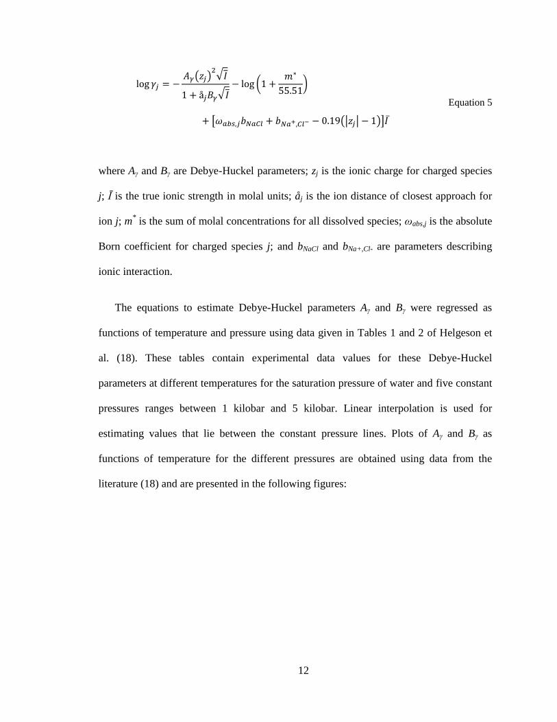
where Aγ and Bγ are Debye-Huckel parameters; zj is the ionic charge for charged species

j; Ī is the true ionic strength in molal units; åj is the ion distance of closest approach for

ion j; m* is the sum of molal concentrations for all dissolved species; ωabs,j is the absolute

Born coefficient for charged species j; and bNaCl and bNa+,Cl- are parameters describing

ionic interaction.

The equations to estimate Debye-Huckel parameters Aγ and Bγ were regressed as

functions of temperature and pressure using data given in Tables 1 and 2 of Helgeson et

al. (18). These tables contain experimental data values for these Debye-Huckel

parameters at different temperatures for the saturation pressure of water and five constant

pressures ranges between 1 kilobar and 5 kilobar. Linear interpolation is used for

estimating values that lie between the constant pressure lines. Plots of Aγ and Bγ as

functions of temperature for the different pressures are obtained using data from the

literature (18) and are presented in the following figures:

13

Figure 1: Debye-Huckel Parameter Aγ as a Function of Temperature at Constant

Pressures

Figure 2: Debye-Huckel Parameter Bγ as a Function of Temperature at Constant

Pressures

0.0

0.2

0.4

0.6

0.8

1.0

1.2

1.4

1.6

1.8

2.0

0 100 200 300 400

Aγ

(kg

1/2

mole

-1/2

)

Temperature (°C)

Debye-Huckel Parameter Aγ

SAT

1 kb

2 kb

3 kb

4 kb

5 kb

0.30

0.35

0.40

0.45

0 100 200 300 400

Bγ

(kg

1/2

mole

-1/2

Ang

-1)

Temperature (°C)

Debye-Huckel Parameter Bγ

SAT

1kb

2kb

3kb

4kb

5kb

14

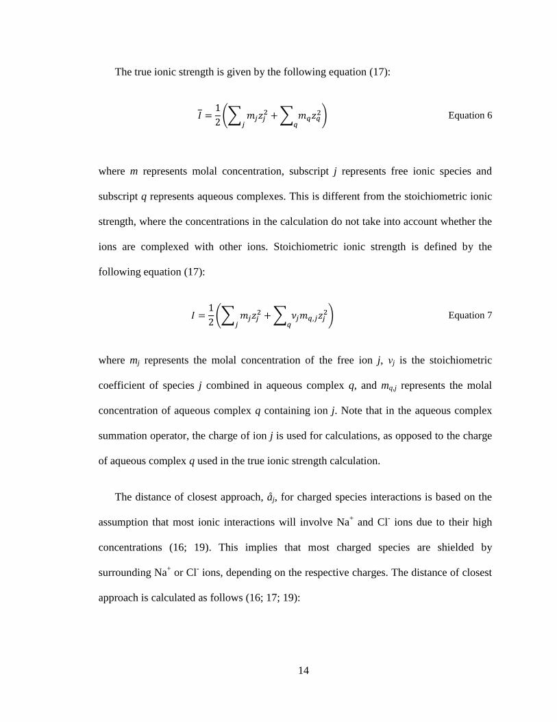
The true ionic strength is given by the following equation (17):

Equation 6

where m represents molal concentration, subscript j represents free ionic species and

subscript q represents aqueous complexes. This is different from the stoichiometric ionic

strength, where the concentrations in the calculation do not take into account whether the

ions are complexed with other ions. Stoichiometric ionic strength is defined by the

following equation (17):

Equation 7

where mj represents the molal concentration of the free ion j, νj is the stoichiometric

coefficient of species j combined in aqueous complex q, and mq,j represents the molal

concentration of aqueous complex q containing ion j. Note that in the aqueous complex

summation operator, the charge of ion j is used for calculations, as opposed to the charge

of aqueous complex q used in the true ionic strength calculation.

The distance of closest approach, åj, for charged species interactions is based on the

assumption that most ionic interactions will involve Na+ and Cl

- ions due to their high

concentrations (16; 19). This implies that most charged species are shielded by

surrounding Na+ or Cl

- ions, depending on the respective charges. The distance of closest

approach is calculated as follows (16; 17; 19):

15

Equation 8

Equation 9

where reff,j is the effective ionic radius of species j in Angstroms. These expressions are

based on simplifications of Equation 125 of Helgeson et al. (17) by Reed (19) as

explained in the TOUGHREACT user guide (16). Values for reff are taken from Table 3

of Helgeson et al. (17). Note that 1.91 and 1.81 are the ionic radii in Angstroms for Na+

and Cl-, respectively.

The absolute Born coefficient for ion j, ωabs,j, is an ion solvation parameter and is

calculated as follows (16; 17):

Equation 10

where η = 1.66027∙105 Ang-cal/mole and reff,j is in Angstroms. It is related to the

dielectric constant of the solution (17).

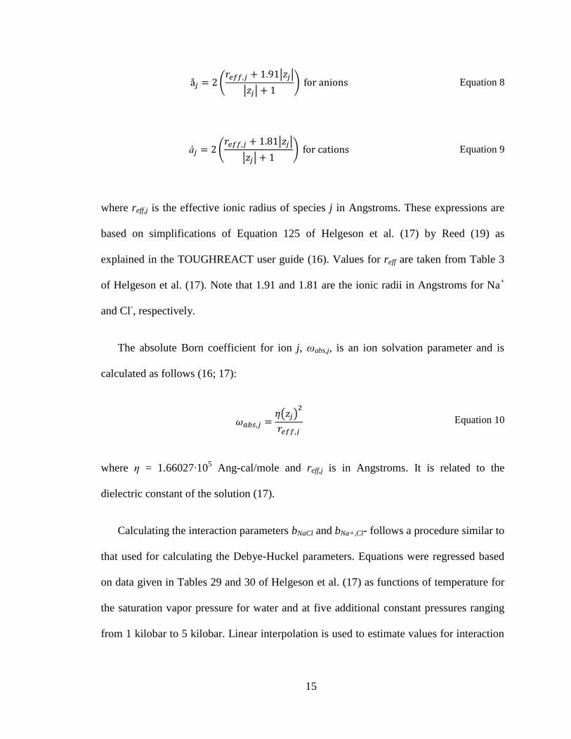
Calculating the interaction parameters bNaCl and bNa+,Cl- follows a procedure similar to

that used for calculating the Debye-Huckel parameters. Equations were regressed based

on data given in Tables 29 and 30 of Helgeson et al. (17) as functions of temperature for

the saturation vapor pressure for water and at five additional constant pressures ranging

from 1 kilobar to 5 kilobar. Linear interpolation is used to estimate values for interaction

16

parameters that lie between constant pressure lines. Plots of bNaCl and bNa+,Cl- are given in

the following figures:

Figure 3: Helgeson Interaction Parameter bNaCl as a Function of Temperature at Constant

Pressures

-12.0

-10.0

-8.0

-6.0

-4.0

-2.0

0.0

2.0

4.0

0 100 200 300 400 500

bN

aC

l(k

g m

ole

-1)*

10

-3

Temperature (°C)

Parameter bNaCl

SAT

1 kb

2 kb

3 kb

4 kb

5 kb

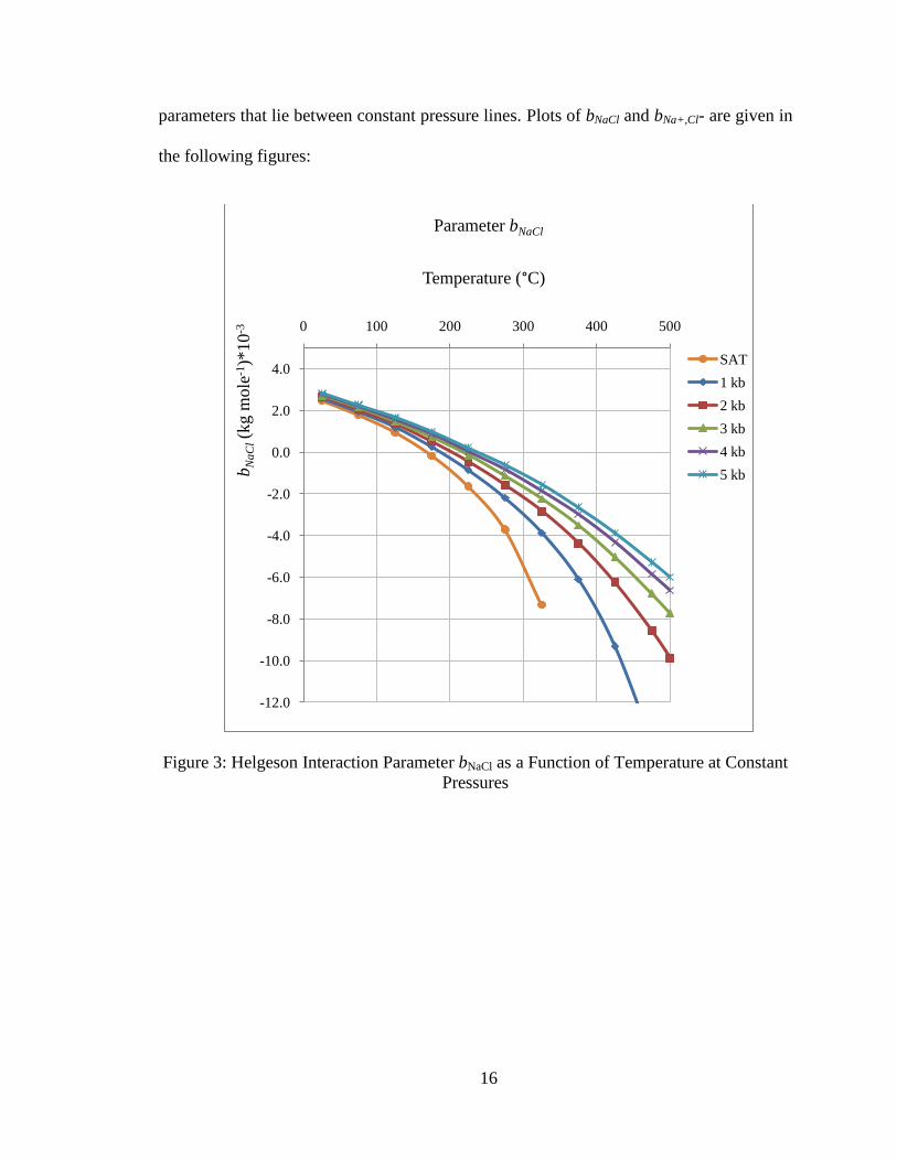
17

Figure 4: Helgeson Interaction Parameter bNa+,Cl- as a Function of Temperature at

Constant Pressures

In summary, Equations 5, 6, and 8-10 are used with data given in Figures 1-4 to

estimate the activity coefficient for each species of dissolved ion and charged aqueous

complex.

3.2.3: Activity Coefficient for Aqueous CO2

The activity coefficient for aqueous (dissolved) CO2 describes the non-ideal effects of

high temperature, pressure, and ionic strength on the chemical activity of CO2(aq). This

-15.0

-10.0

-5.0

0.0

5.0

10.0

15.0

20.0

25.0

30.0

0 100 200 300 400 500

bN

a+

Cl-

(kg m

ole

-1)*

10

-8

Temperature (°C)

Parameter bNa+,Cl-

SAT

1 kb

2 kb

3 kb

4 kb

5 kb

18

coefficient is used to account for the “salting-out” effect that decreases CO2 solubility in

high ionic strength solutions as compared with pure water (16; 20). At low ionic

strengths, the activity coefficient for dissolved CO2 is considered to be unity (16; 21).

However, the activity coefficient increases at high ionic strength as the solution becomes

more “crowded” for dissolved CO2 and dissolution is less than predicted based on ideal

thermodynamic considerations. For this study, three different models are used to estimate

γCO2.

3.2.3.1: Method of Drummond (22)

This model is a function of temperature and ionic strength and is given by the

following expression (16; 22):

Equation 11

where T is the temperature in Kelvin; I is the molal ionic strength; and C, F, G, E and H

are constants tabulated by Drummond (16; 22). This model has been cited in numerous

publications and has been incorporated into TOUGHREACT geochemical modeling

software as well as others (16). This model is valid for a temperature range of 20-400 °C

and 0-6.5 molal NaCl concentration and yields the molal scale activity coefficient for

aqueous CO2 (16; 22).

3.2.3.2: Method of Rumpf et al. (23)

This model is a function of temperature and ionic strength and is given by the

following expression (21; 23):

Equation 12

19

where (21; 23):

Equation 13

and (21; 23):

Equation 14

where T is the temperature in Kelvin and msalt is the molal concentration of all dissolved

salt species. A variation presented by Spycher et al. (21) based on a simplification

presented by Duan et al. (24) is included to yield the final form of the equation (21):

Equation 15

where m is the molal concentration of the indicated species. This method is valid for

temperature from 313-433 K and 0-6 molal salt concentration and yields a molal scale

activity coefficient (21).

3.2.3.3: Method of Duan and Sun (25)

This model is a function of temperature, pressure, and ionic strength, and is given by

the following expression (25):

Equation 16

where λ and ζ are parameters calculated based on the following equation (25):

20

Equation 17

where P is the pressure in bars, T is the temperature in Kelvin, and c1 through c11 are

constants from Table 2 of Duan and Sun (25). Note that λ and ζ use different sets of

constants c1 through c11. This CO2 activity coefficient model is valid for temperatures of

273-573 K, pressures of 0-2000 bar and ionic strengths of 0-4.3 molal (25).

3.3: Estimating the Fugacity Coefficient for Gaseous and Supercritical CO2, φCO2

The fugacity coefficient, φCO2, is a parameter used to describe the deviation from

ideal thermodynamic behavior of gaseous/supercritical CO2 that is observed at high

temperature and pressure. The fugacity coefficient is used to calculate the fugacity of the

CO2(g,sc) phase, a thermodynamic value that is akin to the activity of an aqueous species.

Gas phase fugacity is calculated as follows:

Equation 18

where F is the fugacity, φ is the fugacity coefficient, and PCO2 is the partial pressure of

CO2 in bars. For this study, two models are used to estimate φCO2 as described below.

3.3.1: Method of Spycher and Reed (26)

This model, a function of temperature and pressure, is given by the following

expression (26):

Equation 19

21

where T is the temperature in Kelvin; P is the total gas pressure in bars; and a, b, c, d, e

and f are constants given by Spycher and Reed (26). This model is applicable for a

temperature range of 50-350°C and pressure up to 500 bars (26). It is reported that there

are significant discrepancies between the estimated compressibility factor, Z, using this

model and experimentally observed values of Z at the P-T ranges considered (26). This

indicates that the method of Spycher and Reed (26) might not be the best method for

estimating the CO2 fugacity coefficient. However, this model has been incorporated into

the geochemical modeling software TOUGHREACT (16) and is thus considered in this

thesis.

3.3.2: Method of Duan et al. (20)

This model, also a function of temperature and pressure, is given by the following

expression (20):

Equation 20

where T is the temperature in Kelvin, P is the pressure in bars, and c1 – c15 are constants

given in Table 1 of Duan et al. (20). This model has been fitted to experimental data for

six T-P ranges ranging from 273-573K and 0-2000 bar (20).

3.4: Estimating the Activity of Water, aW

The activity of water, aW, is considered to be unity under ideal conditions. However,

at elevated temperature, pressure, and ionic strength, the activity of water begins to

deviate from unity as a function of the osmotic coefficient, Φ (16; 17):

22

Equation 21

where m* is the total molal concentration of all dissolved ions. The osmotic coefficient,

Φ, is calculated as follows (16):

Equation 22

where (16; 17):

Equation 23

where (16; 17):

Equation 24

where I is the stoichiometric ionic strength (see Equation 7), mt,j is the total molal

concentration of ion j, and mCHRG is the total molal concentration of all charged species in

solution. This procedure for calculating the osmotic coefficient utilizes several

modifications presented in the TOUGHREACT user manual (16). The original form of

the osmotic coefficient equation is Equation 190 of Helgeson et al. (17); and assuming

NaCl dominance in solution, would yield this expression (17):

23

Equation 25

Note that this is a function of the true ionic strength, Ī (see Equation 6). However, it is

reported in the TOUGHREACT user guide (16), and implemented in the

TOUGHREACT program, that using the stoichiometric ionic strength and half the

charged species molality more accurately matches experimentally obtained data than the

original formulation based solely on the true ionic strength (16).

3.5: Aqueous CO2 Concentration, mCO2

The molal concentration of dissolved CO2 in brine is estimated using four methods.

3.5.1: Equilibrium Constant

This method is based on the equilibrium expression for the following chemical

reaction:

Equation 26

Equation 27

where FCO2 is the fugacity of gaseous/supercritical CO2, which is estimated using

techniques discussed in Section 3.3. The activity of bicarbonate ion is constrained

additionally by equilibrium with dissolved CO2 according to the following equations:

24

Equation 28

Equation 29

The value for KCO2(aq) is taken from thermodynamic database included with

TOUGHREACT geochemical modeling software and is calculated as a function of

temperature. At 45°C, the log KCO2(aq) value is -6.273 (16). The activity of CO2(aq) is

related to the molal concentration of CO2 by the following equation:

Equation 30

The equations simplify to yield an expression for mCO2 as a function of CO2 fugacity,

equilibrium constants, and activity coefficient. The concentration of dissolved CO2, along

with the solution pH, is used to estimate the activity of bicarbonate, HCO3-, which all

other geochemical species are functions of. The pH is then iterated until the geochemical

system converges.

3.5.2: Method of Duan and Sun (25)

This model is a function of temperature, pressure and salt content, and is given by

Equation 9 of Duan and Sun (25):

Equation 31

25

where yCO2 is the CO2 mole fraction in the gaseous phase (assumed in this study to be

unity) and μCO21(0)

is the difference between the chemical potentials of CO2 in the gaseous

phase and the liquid phase (20). The value of μCO21(0)

/RT is calculated similarly to λ and ζ

using constants given in Table 2 of Duan and Sun (2003). This CO2 solubility model is

valid for temperatures of 273-573K, pressures of 0-2000 bar and ionic strengths of 0-4.3

m, and yields values that are within 10% of experimentally observed values (20).

3.5.3: Method of Spycher and Pruess (21)

This model is a function of temperature, pressure and salt content, and is given by

Equation 2 of Spycher and Pruess (21):

Equation 32

where yH2O is the water mole fraction in the gaseous phase (assumed to be zero for this

study); γx’ is the mole fraction scale activity coefficient for aqueous CO2; KCO2

0 is the

thermodynamic equilibrium constant for CO2 dissolution; P0 is 1 bar; and is the

average partial molar volume of CO2 over the P0→P range, which is assumed to be 32.6

cm3/mole based on data in Table 2 of Spycher and Pruess (21).

To calculate KCO20, the following equation is used (21):

Equation 33

where a, b, c and d are constants given in Table 2 of Spycher and Pruess (21) and T is

temperature in degrees Celsius.

26

The mole fraction activity coefficient for CO2 can be converted from the molal scale

activity coefficient (see Section 3.2.3:) with the following equation (21):

Equation 34

where msalt is the total molal concentration of all species that are not aqueous CO2 and γm’

is the molal scale activity coefficient that is calculated using methods presented earlier. It

is reported by Spycher and Pruess (21) that more accurate results are obtained using the

methodology of Duan and Sun (25) or Rumpf et al. (23) for calculating γm’.

The molal concentration of aqueous CO2 can be determined from the mole fraction of

aqueous CO2 using the following relationship (21):

Equation 35

Unlike the previous two models for CO2 aqueous solubility, this model requires an

iterative solution. This is due to the need to convert between mole fraction and molal

scales. The solution procedure is as follows:

1.

2.

3.

4.

27

5.

6.

The methodology presented by Spycher and Pruess (21) is valid from 12-100°C, 1-

600 bar and 0-6 molal NaCl concentration (21). However, the iterative procedure is

slightly cumbersome for calculations.

3.5.4: Spycher and Pruess (21) adaptation of the method of Duan and Sun (25)

This methodology is a combination of models presented in Spycher et al. (27) and

Duan and Sun (25) that is presented in Spycher and Pruess (21). If the CO2 solubility

model presented by Duan and Sun (25) is simplified into standard thermodynamic

variables and the natural-log terms are eliminated, the following equation results (21):

Equation 36

where FCO2 is the fugacity of the gaseous CO2 phase, KCO2 is the thermodynamic

equilibrium constant and γCO2 is the activity coefficient of aqueous CO2. Now assume

there are two systems that are identical except that one consists of pure water and the

other system consists of a brine solution with known ionic concentrations.

For pure water (21):

Equation 37

28

For brine (21):

Equation 38

The gas phase fugacity and thermodynamic equilibrium constants are equal because

they are functions of temperature and pressure but not salt content. Thus (21):

Equation 39

However, in pure water, γCO2 approaches unity (16; 21; 27). Thus (21):

Equation 40

Solving for mCO2 (21):

Equation 41

To determine γCO2, the activity coefficient expression presented by Duan and Sun (25)

is used (21), although it appears that any suitable method for estimating γCO2 could

suffice. To determine the solubility of CO2 in pure water, mCO20, the methodology

presented by Spycher et al. (27) is used. This model is given by the following equation

(27):

Equation 42

29

This model for determining solubility in pure water is identical to the model for

determining CO2 solubility (see Equation 32) in brine with the exception of the missing

γx’ term, which is neglected because γx’ approaches unity in pure water (21). Eliminating

the γx’ term makes the solution procedure non-iterative because there is no conversion

from mole fraction to molal scale. All other model parameters are calculated in an

identical fashion to the procedure presented by Spycher and Pruess (21).

3.6: Summary

The parameters discussed in this chapter are used to describe the thermodynamic

environment of a geochemical system. These parameters include solubility equilibrium

constants for mineral precipitation and dissolution, for the formation of aqueous

complexes, and for dissolution of CO2. In addition, non-ideal effects due to high pressure,

salinity, and temperature are accounted for using activity and fugacity coefficients. These

parameters and their methods of estimation are then incorporated into the solution

procedure discussed in Chapter 4 to describe pre- and post-injection conditions for CCS

in a carbonate aquifer.

30

4: Model Development

4.1: Model Overview

Geochemical models are used to estimate the equilibrium concentrations of various

dissolved ions for the purpose of quantifying mineral precipitation and dissolution in

response to CO2 injection. To accomplish this, models were developed to describe both

pre-CO2 injection and post-CO2 injection geochemical conditions. For pre-injection

conditions, the brine pH and salinity (salt mass-fraction) and the aquifer temperature and

pressure are specified parameters and are used to estimate the initial equilibrium

concentrations of dissolved ions. For post-injection conditions, CO2 injection pressure,

aquifer temperature and pressure, and brine salinity are specified parameters and are used

to estimate the new equilibrium pH and ion concentrations. Then, the difference between

pre- and post-injection equilibrium ion concentrations is used to estimate the extent of

mineral precipitation and dissolution and net CO2 solubility trapping that occurs during

thermodynamic equilibrium processes associated with CO2 injection.

4.2: System of Geochemical Equations

The geochemical model is used to solve for the equilibrium concentrations of 28

aqueous species, the activity of water, and the solution net charge. The geochemical

system is non-linear, based on 30 equations and used to solve for 30 unknown values.

This system of equations includes 24 equilibrium expressions for ions and aqueous

31

complexes, two total mass expressions for Na+ and Cl

- ions, three equations to describe

the dissociation and the activity of water, and one charge balance equation that calculates

the net charge of the solution.

4.2.1: Rock Minerals

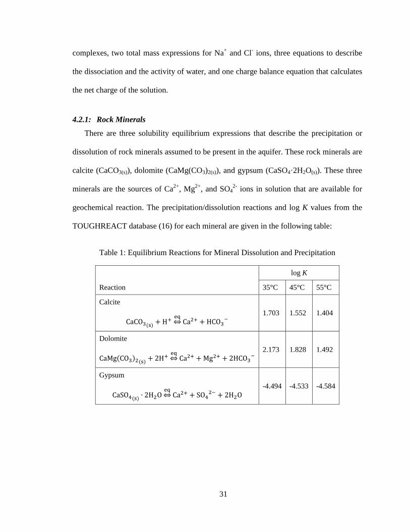
There are three solubility equilibrium expressions that describe the precipitation or

dissolution of rock minerals assumed to be present in the aquifer. These rock minerals are

calcite (CaCO3(s)), dolomite (CaMg(CO3)2(s)), and gypsum (CaSO4·2H2O(s)). These three

minerals are the sources of Ca2+

, Mg2+

, and SO42-

ions in solution that are available for

geochemical reaction. The precipitation/dissolution reactions and log K values from the

TOUGHREACT database (16) for each mineral are given in the following table:

Table 1: Equilibrium Reactions for Mineral Dissolution and Precipitation

Reaction

log K

35°C 45°C 55°C

Calcite

1.703 1.552 1.404

Dolomite

2.173 1.828 1.492

Gypsum

-4.494 -4.533 -4.584

32

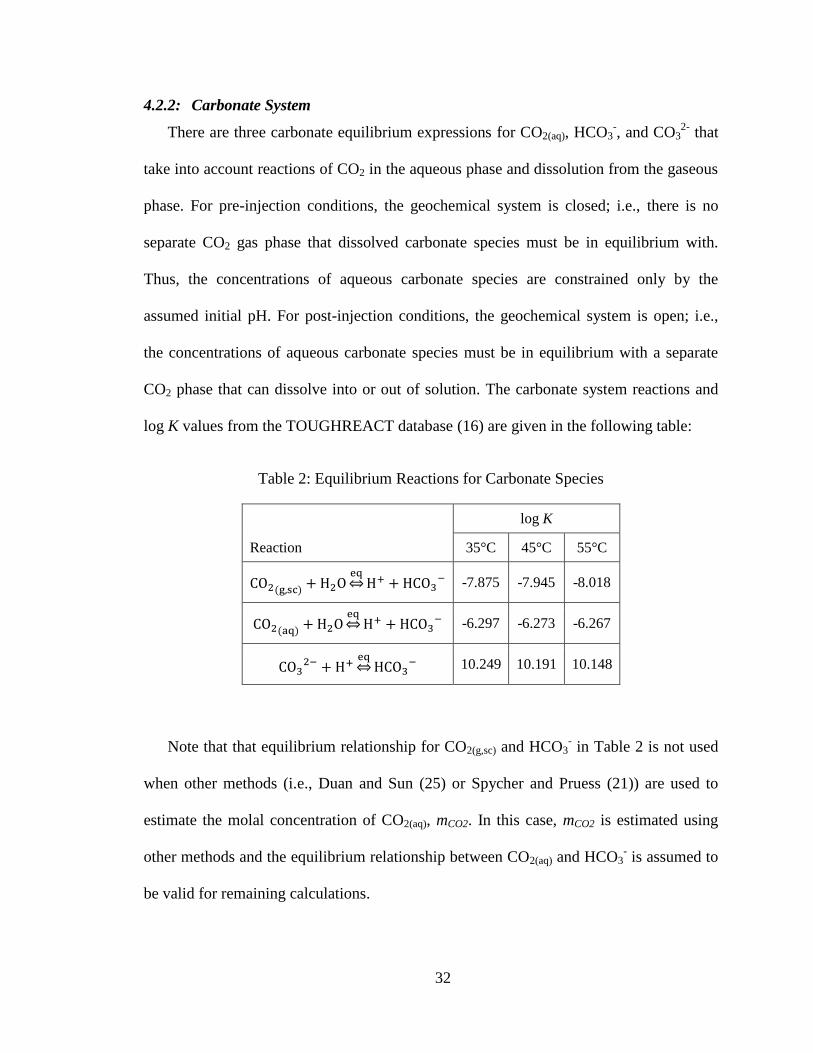
4.2.2: Carbonate System

There are three carbonate equilibrium expressions for CO2(aq), HCO3-, and CO3

2- that

take into account reactions of CO2 in the aqueous phase and dissolution from the gaseous

phase. For pre-injection conditions, the geochemical system is closed; i.e., there is no

separate CO2 gas phase that dissolved carbonate species must be in equilibrium with.

Thus, the concentrations of aqueous carbonate species are constrained only by the

assumed initial pH. For post-injection conditions, the geochemical system is open; i.e.,

the concentrations of aqueous carbonate species must be in equilibrium with a separate

CO2 phase that can dissolve into or out of solution. The carbonate system reactions and

log K values from the TOUGHREACT database (16) are given in the following table:

Table 2: Equilibrium Reactions for Carbonate Species

Reaction

log K

35°C 45°C 55°C

-7.875 -7.945 -8.018

-6.297 -6.273 -6.267

10.249 10.191 10.148

Note that that equilibrium relationship for CO2(g,sc) and HCO3- in Table 2 is not used

when other methods (i.e., Duan and Sun (25) or Spycher and Pruess (21)) are used to

estimate the molal concentration of CO2(aq), mCO2. In this case, mCO2 is estimated using

other methods and the equilibrium relationship between CO2(aq) and HCO3- is assumed to

be valid for remaining calculations.

33

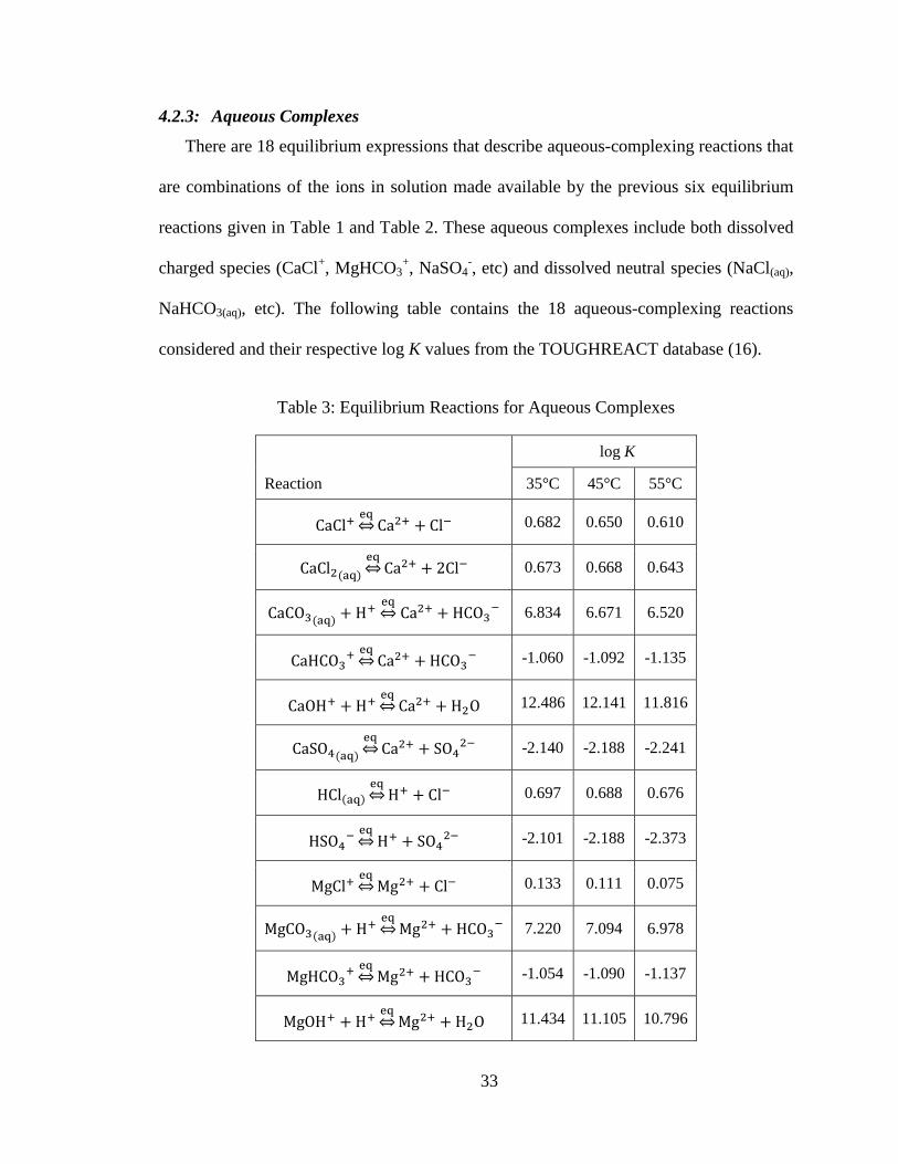
4.2.3: Aqueous Complexes

There are 18 equilibrium expressions that describe aqueous-complexing reactions that

are combinations of the ions in solution made available by the previous six equilibrium

reactions given in Table 1 and Table 2. These aqueous complexes include both dissolved

charged species (CaCl+, MgHCO3

+, NaSO4

-, etc) and dissolved neutral species (NaCl(aq),

NaHCO3(aq), etc). The following table contains the 18 aqueous-complexing reactions

considered and their respective log K values from the TOUGHREACT database (16).

Table 3: Equilibrium Reactions for Aqueous Complexes

Reaction

log K

35°C 45°C 55°C

0.682 0.650 0.610

0.673 0.668 0.643

6.834 6.671 6.520

-1.060 -1.092 -1.135

12.486 12.141 11.816

-2.140 -2.188 -2.241

0.697 0.688 0.676

-2.101 -2.188 -2.373

0.133 0.111 0.075

7.220 7.094 6.978

-1.054 -1.090 -1.137

11.434 11.105 10.796

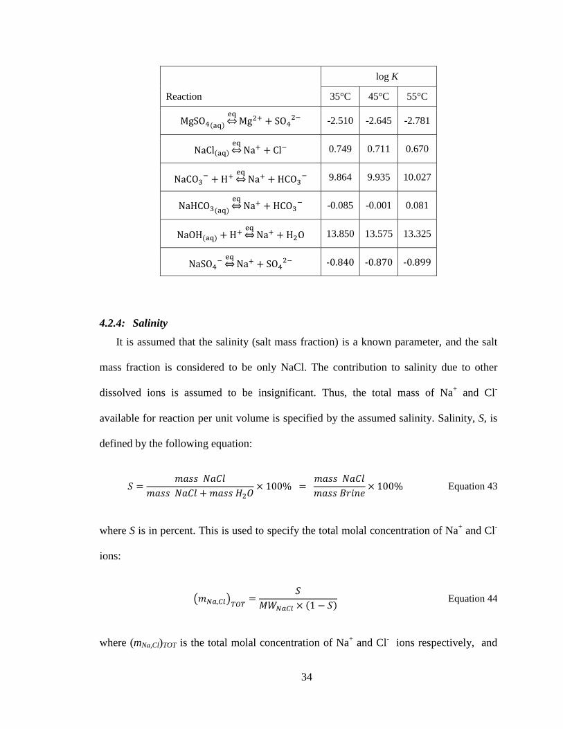
34

Reaction

log K

35°C 45°C 55°C

-2.510 -2.645 -2.781

0.749 0.711 0.670

9.864 9.935 10.027

-0.085 -0.001 0.081

13.850 13.575 13.325

-0.840 -0.870 -0.899

4.2.4: Salinity

It is assumed that the salinity (salt mass fraction) is a known parameter, and the salt

mass fraction is considered to be only NaCl. The contribution to salinity due to other

dissolved ions is assumed to be insignificant. Thus, the total mass of Na+ and Cl

-

available for reaction per unit volume is specified by the assumed salinity. Salinity, S, is

defined by the following equation:

Equation 43

where S is in percent. This is used to specify the total molal concentration of Na+ and Cl

-

ions:

Equation 44

where (mNa,Cl)TOT is the total molal concentration of Na+ and Cl

- ions respectively, and

35

MWNaCl is the formula weight for NaCl (58.443*10-3

kg/mole). Note that this equation is

applied twice in the geochemical model to determine the concentrations of both Na+ and

Cl-. This is used as a constraint for all species containing Na

+ and Cl

- because the sum of

concentration of Na+ and Cl

- in all species containing Na

+ and Cl

- must equal the total

concentrations for Na+ and Cl

- specified by the known salt mass-fraction.

4.2.5: Water (H2O) System

The dissociation of water (H2O) into H+ and OH

- ions must be considered for any

system contained within the aqueous phase. The water dissociation reaction and log K

values from the TOUGHREACT database (16) are given in the following table:

Table 4: Equilibrium Reactions for H2O Dissociation

Reaction

log K

35°C 45°C 55°C

13.680 13.400 13.146

The activities of H+ and OH

- are related to the activity of H2O (see Chapter 3.4) by

the following expression:

Equation 45

The pH of the brine is related to the chemical activity of H+ by the following

equation:

Equation 46

36

4.2.6: Charge Balance

The charge balance equation quantifies the net charge of the solution. It is the sum of

the concentrations all ionic and complexed species multiplied by their respective overall

charge:

Equation 47

where m indicates molal concentration, z indicates charge, subscript j indicates ions and

subscript q indicates aqueous complexes.

4.3: Iterative Solution Procedure

Because the system of equations is non-linear, an iterative solution procedure is

required. In this iterative procedure, a basis species from the parent reactions that appears

often in the system of equilibrium equations is chosen. The basis species is chosen in

such a way that all other geochemical species are functions of this species and its value

can be conveniently iterated until all equations are satisfied. Essentially, this means

picking a basis species that is not specified by any known parameters. The molal

concentration of this basis species is then iterated until the net solution charge converges

to zero (within an allowable tolerance). For initial conditions (pre-injection), the basis

species is bicarbonate ion, HCO3-, because it is not constrained solely by any specified

parameter (i.e. initial pH, aquifer pressure, salinity, or temperature). For calculations after

CO2 injection occurs, H+ is the chosen basis species because the pH is no longer specified

and the activity of HCO3- is now constrained by equilibrium with the gaseous CO2 phase.

The solution procedure consists of an inner iteration loop and an outer iteration loop

which are discussed below.

37

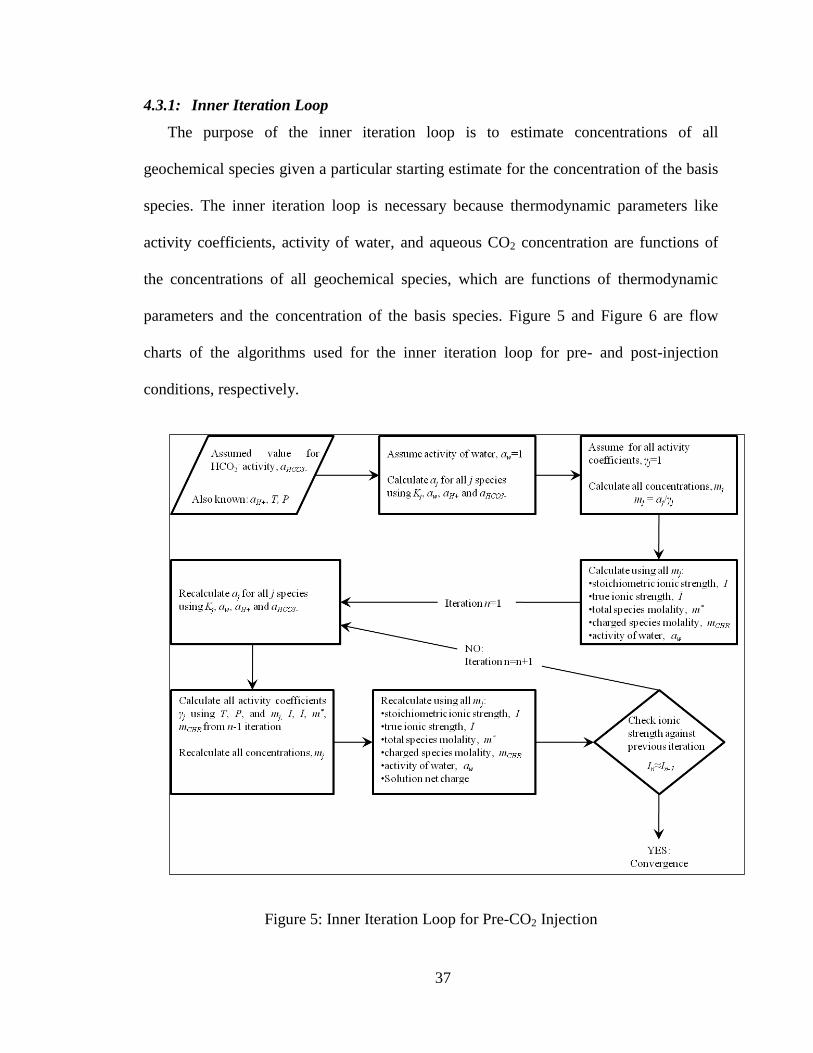
4.3.1: Inner Iteration Loop

The purpose of the inner iteration loop is to estimate concentrations of all

geochemical species given a particular starting estimate for the concentration of the basis

species. The inner iteration loop is necessary because thermodynamic parameters like

activity coefficients, activity of water, and aqueous CO2 concentration are functions of

the concentrations of all geochemical species, which are functions of thermodynamic

parameters and the concentration of the basis species. Figure 5 and Figure 6 are flow

charts of the algorithms used for the inner iteration loop for pre- and post-injection

conditions, respectively.

Figure 5: Inner Iteration Loop for Pre-CO2 Injection

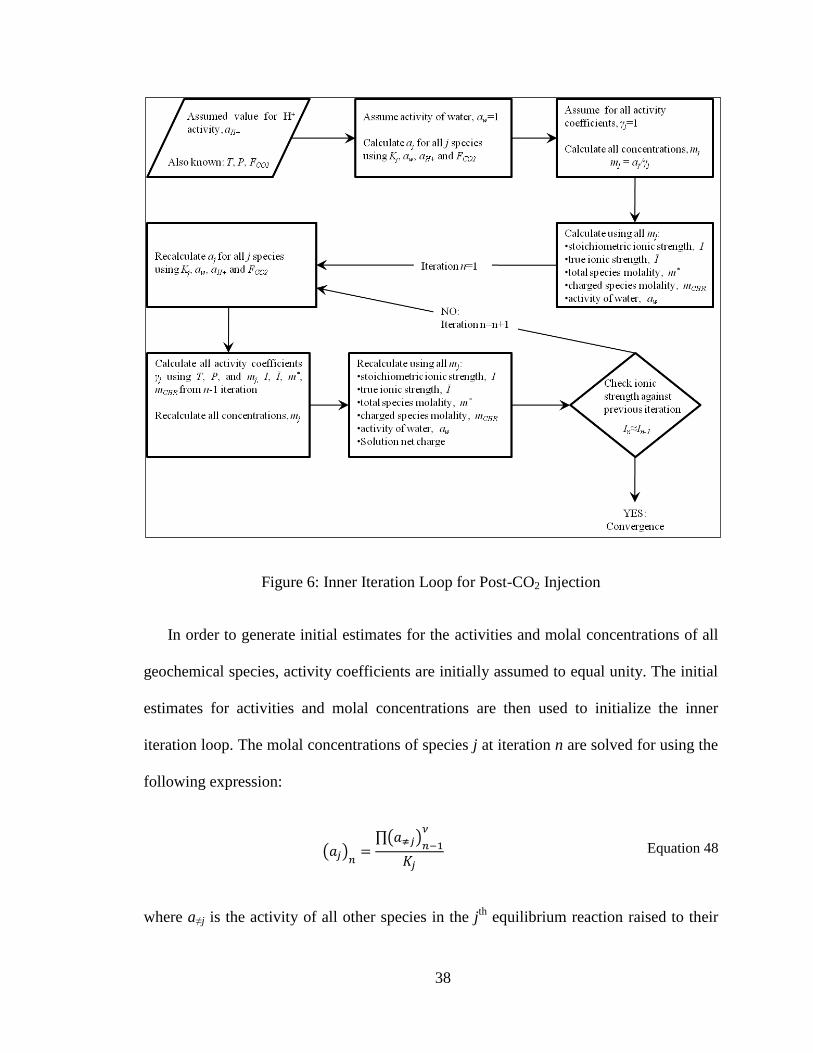
38

Figure 6: Inner Iteration Loop for Post-CO2 Injection

In order to generate initial estimates for the activities and molal concentrations of all

geochemical species, activity coefficients are initially assumed to equal unity. The initial

estimates for activities and molal concentrations are then used to initialize the inner

iteration loop. The molal concentrations of species j at iteration n are solved for using the

following expression:

Equation 48

where a≠j is the activity of all other species in the jth

equilibrium reaction raised to their

39

respective stoichiometric coefficient ν, and Kj is the equilibrium constant for the jth

equilibrium reaction (as given in Tables 1-4).

The activity of species j is used to estimate the concentration of species j at iteration n

with the following expression:

Equation 49

where γj is the activity coefficient for species j. The activity coefficient for the jth

ion at

iteration n is estimated using concentrations and the ionic strength from the previous

iteration:

Equation 50

The procedure is similar for estimating the activity of water at the nth

iteration:

Equation 51

To solve for the concentrations of free Na+ and Cl

- ions at iteration n, the following

expressions are used:

Equation 52

Equation 53

40

where m indicates molal concentration and (mNa+)q and (mCl-)q indicate molal

concentration of Na+ and Cl

- in aqueous complex q multiplied by their stoichiometric

coefficient ν, respectively. These concentrations for free Na+ and Cl

- ions are then used to

solve for the activities of aqueous complexes containing Na+ and Cl

- ions for iteration n.

The inner iteration loop is considered to have converged when the change in ionic

strength between successive iterations is less than a specified tolerance. A minimal

change in ionic strength between iterations indicates that a stable solution has been

determined for the given basis species activity.

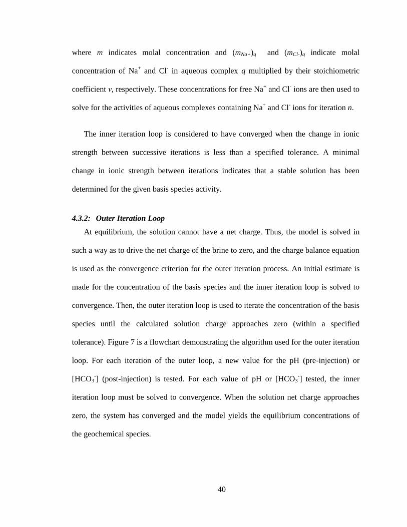
4.3.2: Outer Iteration Loop

At equilibrium, the solution cannot have a net charge. Thus, the model is solved in

such a way as to drive the net charge of the brine to zero, and the charge balance equation

is used as the convergence criterion for the outer iteration process. An initial estimate is

made for the concentration of the basis species and the inner iteration loop is solved to

convergence. Then, the outer iteration loop is used to iterate the concentration of the basis

species until the calculated solution charge approaches zero (within a specified

tolerance). Figure 7 is a flowchart demonstrating the algorithm used for the outer iteration

loop. For each iteration of the outer loop, a new value for the pH (pre-injection) or

[HCO3-] (post-injection) is tested. For each value of pH or [HCO3

-] tested, the inner

iteration loop must be solved to convergence. When the solution net charge approaches

zero, the system has converged and the model yields the equilibrium concentrations of

the geochemical species.

41

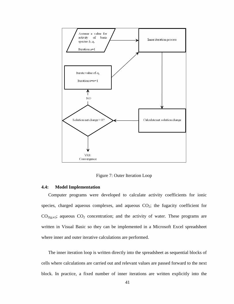
Figure 7: Outer Iteration Loop

4.4: Model Implementation

Computer programs were developed to calculate activity coefficients for ionic

species, charged aqueous complexes, and aqueous CO2; the fugacity coefficient for

CO2(g,sc); aqueous CO2 concentration; and the activity of water. These programs are

written in Visual Basic so they can be implemented in a Microsoft Excel spreadsheet

where inner and outer iterative calculations are performed.

The inner iteration loop is written directly into the spreadsheet as sequential blocks of

cells where calculations are carried out and relevant values are passed forward to the next

block. In practice, a fixed number of inner iterations are written explicitly into the

42

structure of the spreadsheet. Excess iterations are written into the spreadsheet to ensure

that the inner loop will converge for a given estimate of the basis species concentration.

In most cases, fewer than ten inner iterations are required per outer iteration, and 20 inner

iterations are sufficient in all scenarios examined. The outer loop is iterated using the

SOLVER function that is included in Microsoft Excel. The SOLVER function iterates the

concentration of the basis species until the convergence criterion of net solution charge

approaching zero is met.

4.5: Model Limitations

The geochemical model is based on the assumption of system equilibrium for both

pre- and post-CO2 injection conditions. The model only examines geochemistry in the

residual brine saturation and does not address chemical processes that occur at the

moving CO2-brine interface. The model also assumes the presence of only three minerals:

calcite, dolomite, and gypsum. The model is based on the assumption that only these

three minerals are allowed to dissolve and/or precipitate. Finally, the model does not

address advective/transport effects or chemical reaction rates.

4.6: Model Outputs

Once solved, the geochemical model yields the concentrations and activity

coefficients of all aqueous species included in the system, the activity of water, and the

CO2(g,sc) fugacity for post-injection conditions. Next, the amount of minerals that

precipitate or dissolve due to CO2 injection can be estimated by examining the difference

in concentrations of calcium, magnesium, and sulfate ions in solution for pre- and post-

injection conditions. Positive concentration difference indicates that ions enter solution

43

due to mineral dissolution, and negative concentration difference indicates that ions leave

solution due to mineral precipitation. Thus:

Equation 54

Equation 55

Equation 56

where m indicates molal concentration and subscripts pre and post refer to conditions

before and after CO2 injection, respectively.

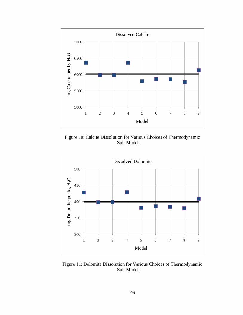
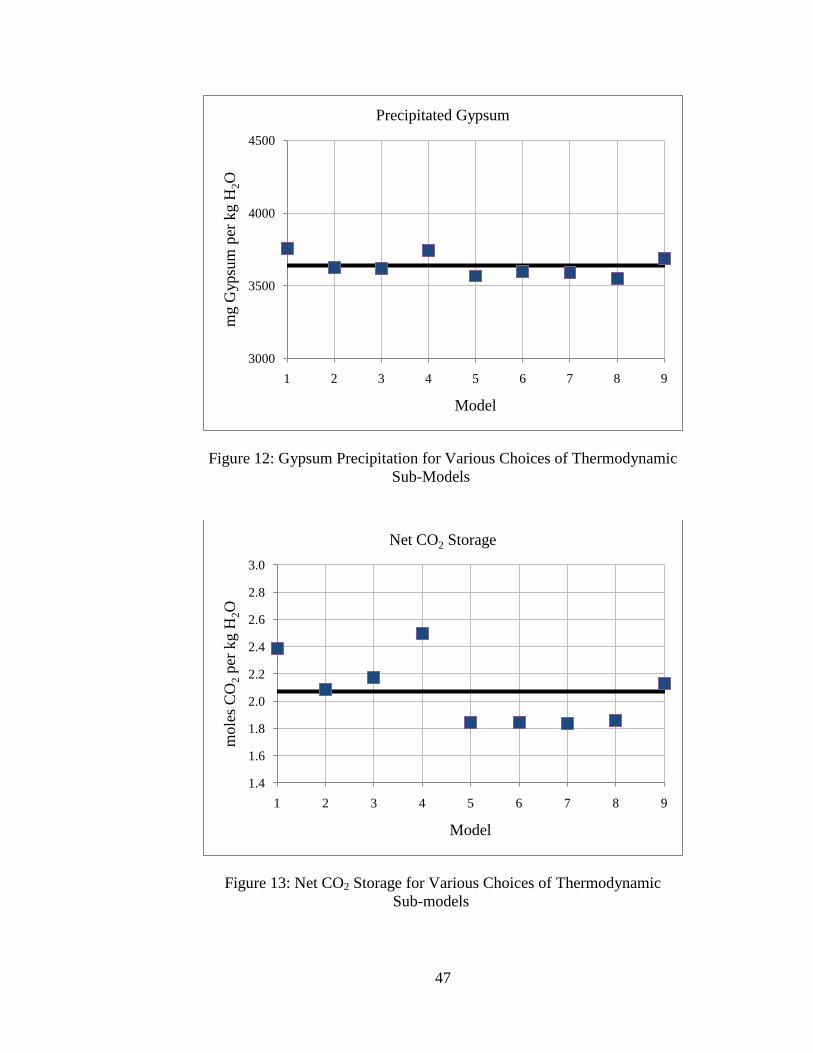
Changes in concentrations of carbonate species can also be used to estimate the net

CO2 storage via the solubility trapping mechanism:

Equation 57

4.7: Comparison of Thermodynamic Sub-models

With three different models for estimating γCO2, two models for estimating φCO2, and

four models for estimating mCO2, as described in Chapter 3, there are 24 possible

combinations of thermodynamic sub-models that could be studied. Initially, nine overall

geochemical models were developed using different combinations of the thermodynamic

models, as summarized in Table 5.

44

Table 5: Combinations of Sub-Models for CO2 Thermodynamic Parameter Estimation

Model

Sub-models for CO2 thermodynamic parameter estimation

CO2(aq)

Activity Coefficient

CO2(g,sc)

Fugacity Coefficient CO2(aq) Solubility

1 Drummond (22) Spycher and Reed (26) Equilibrium Constant (16)

2 Drummond (22) Duan and Sun (20) Equilibrium Constant (16)

3 Rumpf et al. (23) Duan and Sun (20) Equilibrium Constant (16)

4 Rumpf et al. (1994) Spycher and Reed (20) Equilibrium Constant (16)

5 Duan and Sun (2003) Duan et al. (20) Duan and Sun (25)

6 Drummond (22) Duan et al. (20) Duan and Sun (25)

7

Drummond (22) Duan et al. (20)

Spycher and Pruess (21)

adaptation of Duan and Sun

(25)

8 Rumpf et al. (23) Duan et al. (20) Spycher and Pruess (21)

9 Rumpf et al. (23) Spycher and Reed (26) Spycher and Pruess (21)

These nine combinations of thermodynamic sub-models were then used to examine a

baseline geochemical scenario to determine the sensitivity of model outputs to the choice

of thermodynamic sub-models. The baseline geochemical scenario has an initial pH of

7.5, brine salinity of 10%, initial aquifer pressure of 100 bar, CO2 injection pressure of

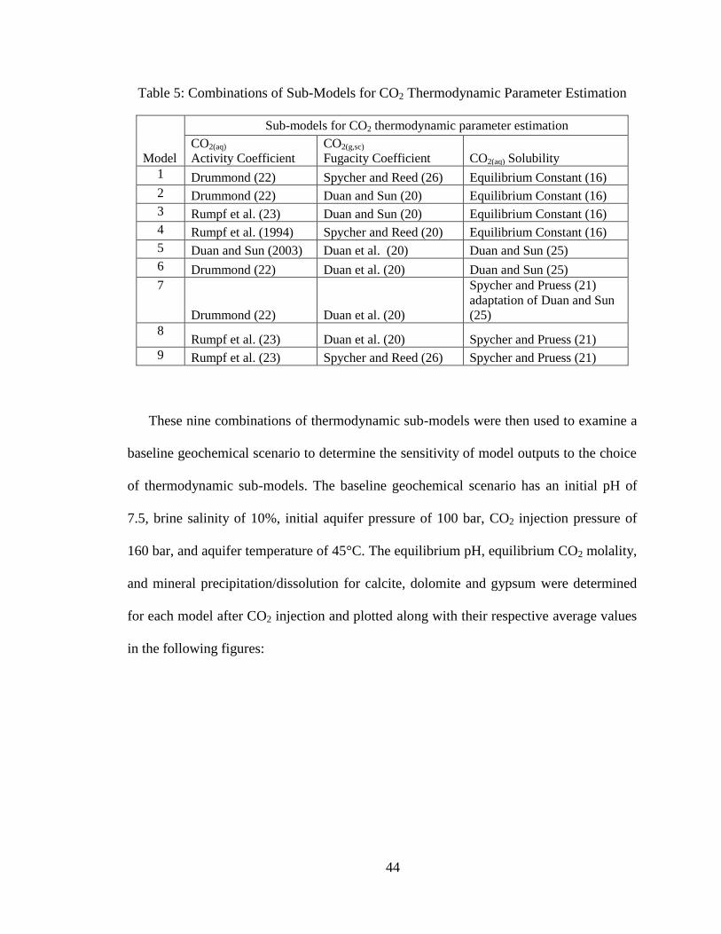
160 bar, and aquifer temperature of 45°C. The equilibrium pH, equilibrium CO2 molality,

and mineral precipitation/dissolution for calcite, dolomite and gypsum were determined

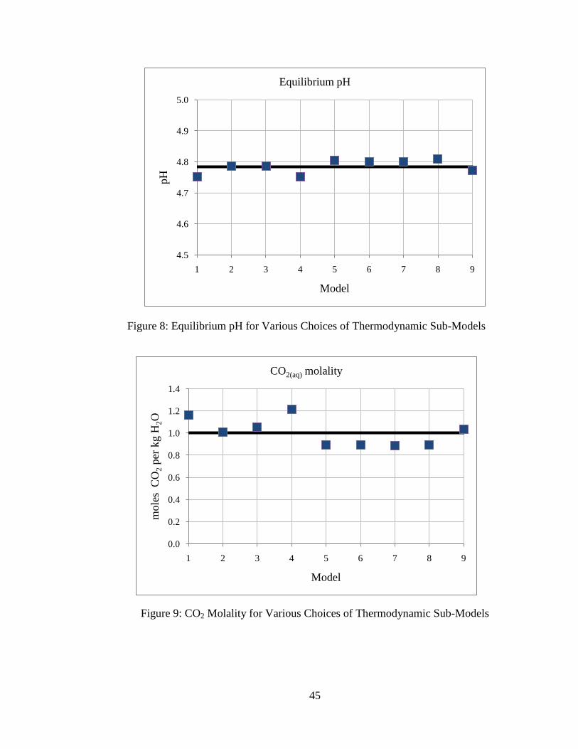
for each model after CO2 injection and plotted along with their respective average values

in the following figures:

45

Figure 8: Equilibrium pH for Various Choices of Thermodynamic Sub-Models

Figure 9: CO2 Molality for Various Choices of Thermodynamic Sub-Models

4.5

4.6

4.7

4.8

4.9

5.0

1 2 3 4 5 6 7 8 9

pH

Model

Equilibrium pH

0.0

0.2

0.4

0.6

0.8

1.0

1.2

1.4

1 2 3 4 5 6 7 8 9

mole

s C

O2

per

kg H

2O

Model

CO2(aq) molality

46

Figure 10: Calcite Dissolution for Various Choices of Thermodynamic

Sub-Models

Figure 11: Dolomite Dissolution for Various Choices of Thermodynamic

Sub-Models

5000

5500

6000

6500

7000

1 2 3 4 5 6 7 8 9

mg C

alci

te p

er k

g H

2O

Model

Dissolved Calcite

300

350

400

450

500

1 2 3 4 5 6 7 8 9

mg D

olo

mit

e per

kg H

2O

Model

Dissolved Dolomite

47

Figure 12: Gypsum Precipitation for Various Choices of Thermodynamic

Sub-Models

Figure 13: Net CO2 Storage for Various Choices of Thermodynamic

Sub-models

3000

3500

4000

4500

1 2 3 4 5 6 7 8 9

mg G

ypsu

m p

er k

g H

2O

Model

Precipitated Gypsum

1.4

1.6

1.8

2.0

2.2

2.4

2.6

2.8

3.0

1 2 3 4 5 6 7 8 9

mole

s C

O2

per

kg H

2O

Model

Net CO2 Storage

48

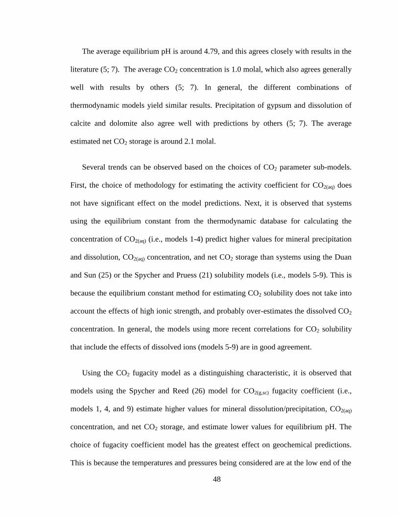
The average equilibrium pH is around 4.79, and this agrees closely with results in the

literature (5; 7). The average CO2 concentration is 1.0 molal, which also agrees generally

well with results by others (5; 7). In general, the different combinations of

thermodynamic models yield similar results. Precipitation of gypsum and dissolution of

calcite and dolomite also agree well with predictions by others (5; 7). The average

estimated net CO2 storage is around 2.1 molal.

Several trends can be observed based on the choices of CO2 parameter sub-models.

First, the choice of methodology for estimating the activity coefficient for CO2(aq) does

not have significant effect on the model predictions. Next, it is observed that systems

using the equilibrium constant from the thermodynamic database for calculating the

concentration of CO2(aq) (i.e., models 1-4) predict higher values for mineral precipitation

and dissolution, CO2(aq) concentration, and net CO2 storage than systems using the Duan

and Sun (25) or the Spycher and Pruess (21) solubility models (i.e., models 5-9). This is

because the equilibrium constant method for estimating CO2 solubility does not take into

account the effects of high ionic strength, and probably over-estimates the dissolved CO2

concentration. In general, the models using more recent correlations for CO2 solubility

that include the effects of dissolved ions (models 5-9) are in good agreement.

Using the CO2 fugacity model as a distinguishing characteristic, it is observed that

models using the Spycher and Reed (26) model for CO2(g,sc) fugacity coefficient (i.e.,

models 1, 4, and 9) estimate higher values for mineral dissolution/precipitation, CO2(aq)

concentration, and net CO2 storage, and estimate lower values for equilibrium pH. The

choice of fugacity coefficient model has the greatest effect on geochemical predictions.

This is because the temperatures and pressures being considered are at the low end of the

49

recommended ranges for use with the Spycher and Reed model where inaccuracies are

reported for fugacity coefficient estimation (26). The fugacity coefficient model

presented by Duan et al. (20) is fitted to experimental data for six different T-P regimes

and probably a better choice for the conditions considered.

However, the differences in geochemical predictions are generally low – estimates

from all models for the equilibrium pH agree to within ±1% of the average, estimates

from all models for mineral precipitation and dissolution agree to within ±10% of the

average, and estimates from all models for mCO2 and net CO2 storage agree to within

±25% of the average. This suggests that the choice of thermodynamic sub-models for

estimating CO2 parameters does not have a large effect on the solution to the geochemical

system. Additionally, these results suggest that variations in estimated CO2 solubility

have a limited effect on other estimated quantities like equilibrium pH and mineral

precipitation or dissolution.

From these nine geochemical systems, three were chosen such that each model used

different sub-models for calculating mCO2 and γCO2. The models chosen for further

investigation are models 1, 5, and 8 from the preceding table. These models are used to

examine the sensitivity of the system to key chemical and physical parameters as

described in the next chapter.

50

5: Model Results

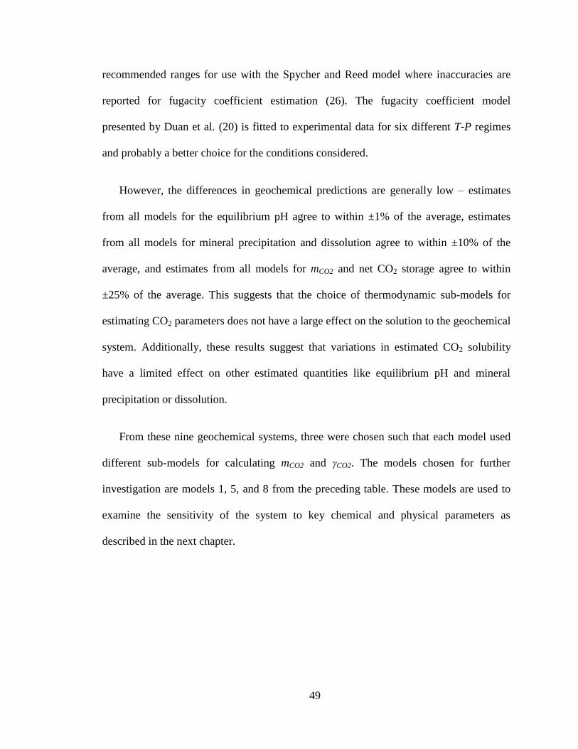
Models 1, 5 and 8 are used to examine the effects of initial pH, CO2 injection

pressure, salinity, and temperature on the geochemical system. Simulations are performed

such that one parameter varies while the other three are kept constant in order to evaluate

the sensitivity of the geochemical system to the varying parameter. These simulations are

variants of the base case described in Chapter 4 where the initial pH is 7.5, aquifer

pressure is 100 bar, CO2 injection pressure is 160 bar, salinity is 10%, and temperature is

45°C.

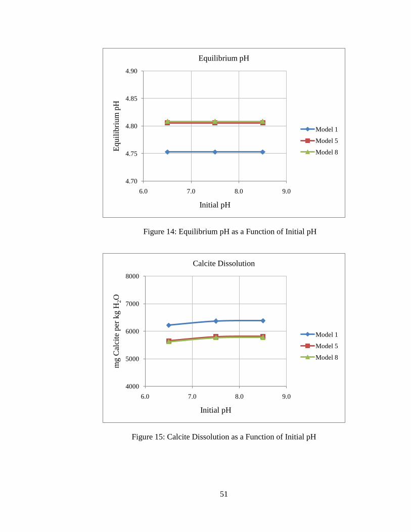
5.1: Effect of Initial pH

In these simulations, temperature, CO2 injection pressure and salinity are constant at

45°C, 160 bar and 10%, respectively. Three sets of simulations using an initial pH of 6.5,

7.5, and 8.5 were performed.

51

Figure 14: Equilibrium pH as a Function of Initial pH

Figure 15: Calcite Dissolution as a Function of Initial pH

4.70

4.75

4.80

4.85

4.90

6.0 7.0 8.0 9.0

Equil

ibri

um

pH

Initial pH

Equilibrium pH

Model 1

Model 5

Model 8

4000

5000

6000

7000

8000

6.0 7.0 8.0 9.0

mg C

alci

te p

er k

g H

2O

Initial pH

Calcite Dissolution

Model 1

Model 5

Model 8

52

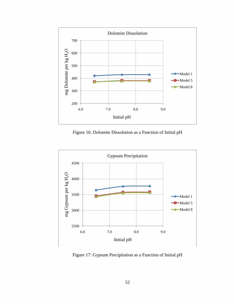
Figure 16: Dolomite Dissolution as a Function of Initial pH

Figure 17: Gypsum Precipitation as a Function of Initial pH

200

300

400

500

600

700

6.0 7.0 8.0 9.0

mg D

olo

mit

e per

kg H

2O

Initial pH

Dolomite Dissolution

Model 1

Model 5

Model 8

2500

3000

3500

4000

4500

6.0 7.0 8.0 9.0

mg G

ypsu

m p

er k

g H

2O

Initial pH

Gypsum Precipitation

Model 1

Model 5

Model 8

53

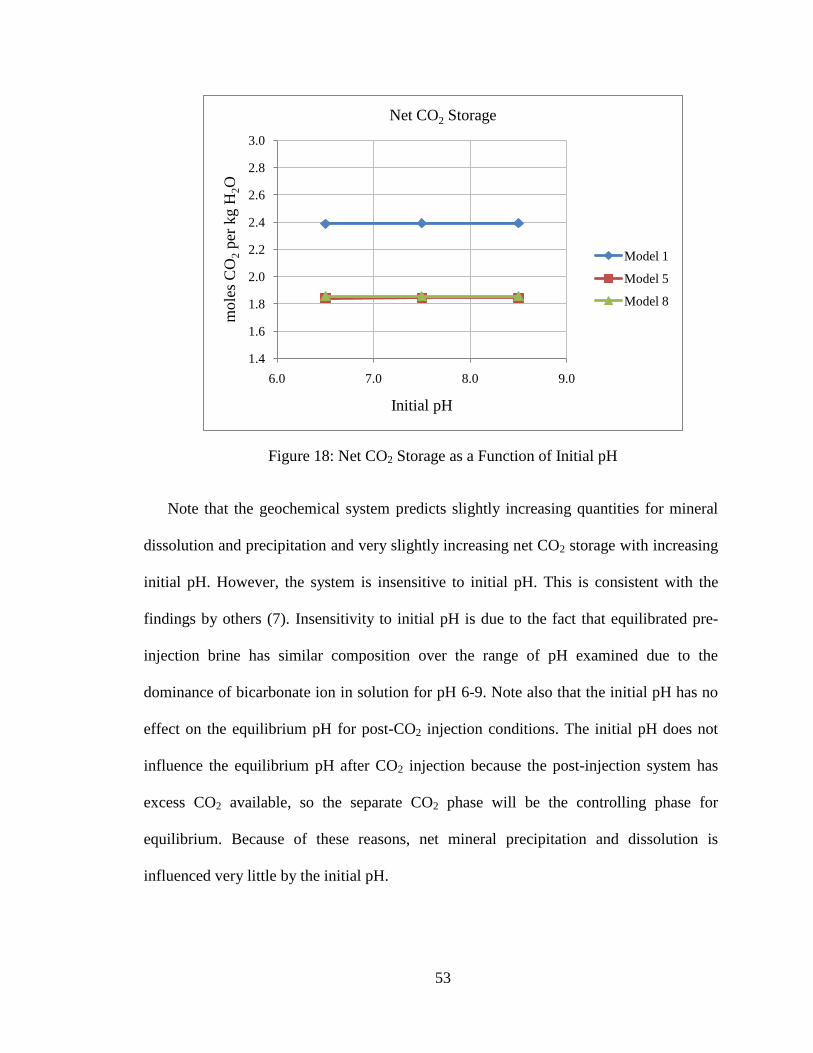
Figure 18: Net CO2 Storage as a Function of Initial pH

Note that the geochemical system predicts slightly increasing quantities for mineral

dissolution and precipitation and very slightly increasing net CO2 storage with increasing

initial pH. However, the system is insensitive to initial pH. This is consistent with the

findings by others (7). Insensitivity to initial pH is due to the fact that equilibrated pre-

injection brine has similar composition over the range of pH examined due to the

dominance of bicarbonate ion in solution for pH 6-9. Note also that the initial pH has no

effect on the equilibrium pH for post-CO2 injection conditions. The initial pH does not

influence the equilibrium pH after CO2 injection because the post-injection system has

excess CO2 available, so the separate CO2 phase will be the controlling phase for

equilibrium. Because of these reasons, net mineral precipitation and dissolution is

influenced very little by the initial pH.

1.4

1.6

1.8

2.0

2.2

2.4

2.6

2.8

3.0

6.0 7.0 8.0 9.0

mole

s C

O2

per

kg H

2O

Initial pH

Net CO2 Storage

Model 1

Model 5

Model 8

54

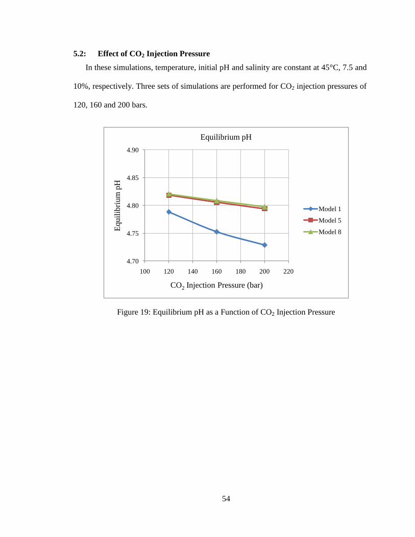
5.2: Effect of CO2 Injection Pressure

In these simulations, temperature, initial pH and salinity are constant at 45°C, 7.5 and

10%, respectively. Three sets of simulations are performed for CO2 injection pressures of

120, 160 and 200 bars.

Figure 19: Equilibrium pH as a Function of CO2 Injection Pressure

4.70

4.75

4.80

4.85

4.90

100 120 140 160 180 200 220

Equil

ibri

um

pH

CO2 Injection Pressure (bar)

Equilibrium pH

Model 1

Model 5

Model 8

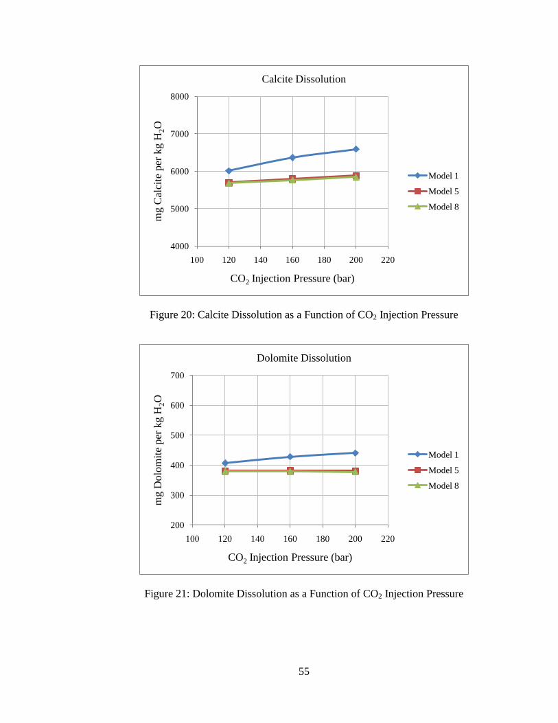
55

Figure 20: Calcite Dissolution as a Function of CO2 Injection Pressure

Figure 21: Dolomite Dissolution as a Function of CO2 Injection Pressure

4000

5000

6000

7000

8000

100 120 140 160 180 200 220

mg C

alci

te p

er k

g H

2O


Calcite Dissolution

Model 1

Model 5

Model 8

200

300

400

500

600

700

100 120 140 160 180 200 220

mg D

olo

mit

e per

kg H

2O



Model 1

Model 5

Model 8

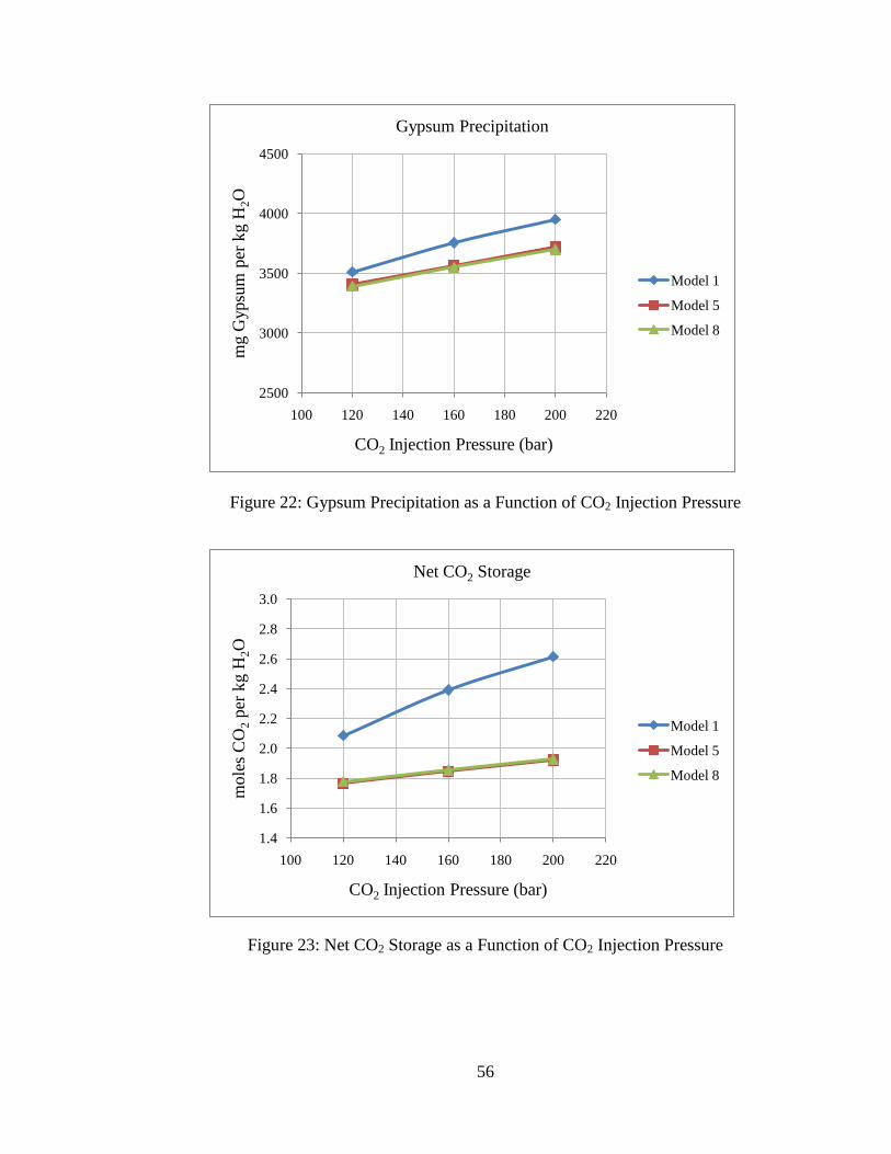
56

Figure 22: Gypsum Precipitation as a Function of CO2 Injection Pressure

Figure 23: Net CO2 Storage as a Function of CO2 Injection Pressure

2500

3000

3500

4000

4500

100 120 140 160 180 200 220

mg G

ypsu

m p

er k

g H

2O



Model 1

Model 5

Model 8

1.4

1.6

1.8

2.0

2.2

2.4

2.6

2.8

3.0

100 120 140 160 180 200 220

mole

s C

O2

per

kg H

2O


Net CO2 Storage

Model 1

Model 5

Model 8

57

Note that the geochemical system predicts slightly increasing quantities of mineral

dissolution and precipitation, decreased equilibrium pH, and increased net CO2 storage in

response to increasing CO2 injection pressure. However, the system is relatively

insensitive to CO2 injection pressure. This is due to the fact that the fugacity of the

CO2(g,sc) phase does not vary proportionally with pressure over the range of pressures

examined. Using the baseline scenario and the Spycher and Reed (26) methodology for

estimating CO2 fugacity, varying the pressure from 120 bar to 200 bar results in a change

in fugacity from 70 to 88 bar; i.e. a 67% increase in pressure results in a 26% increase in

fugacity. Similarly, using the Duan et al. (20) methodology for estimating CO2 fugacity,

the same 67% increase in pressure results in a 19% increase in CO2 fugacity. This

minimizes the effects of increased CO2 pressure on the concentrations of carbonate

species.

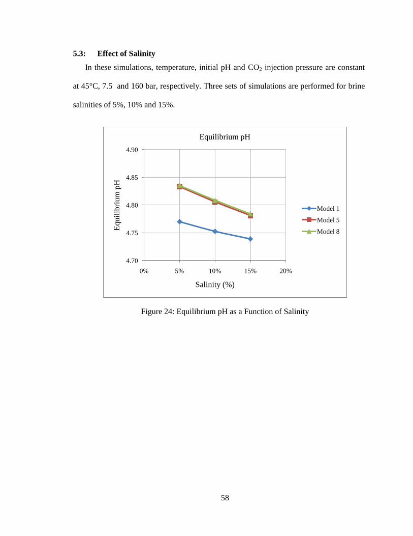
58

5.3: Effect of Salinity

In these simulations, temperature, initial pH and CO2 injection pressure are constant

at 45°C, 7.5 and 160 bar, respectively. Three sets of simulations are performed for brine

salinities of 5%, 10% and 15%.

Figure 24: Equilibrium pH as a Function of Salinity

4.70

4.75

4.80

4.85

4.90

0% 5% 10% 15% 20%

Equil

ibri

um

pH

Salinity (%)

Equilibrium pH

Model 1

Model 5

Model 8

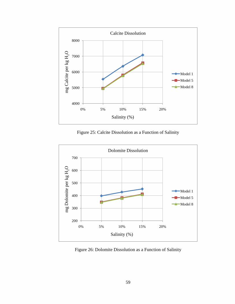
59

Figure 25: Calcite Dissolution as a Function of Salinity

Figure 26: Dolomite Dissolution as a Function of Salinity

4000

5000

6000

7000

8000

0% 5% 10% 15% 20%

mg C

alci

te p

er k

g H

2O

Salinity (%)

Calcite Dissolution

Model 1

Model 5

Model 8

200

300

400

500

600

700

0% 5% 10% 15% 20%

mg D

olo

mit

e per

kg H

2O

Salinity (%)


Model 1

Model 5

Model 8

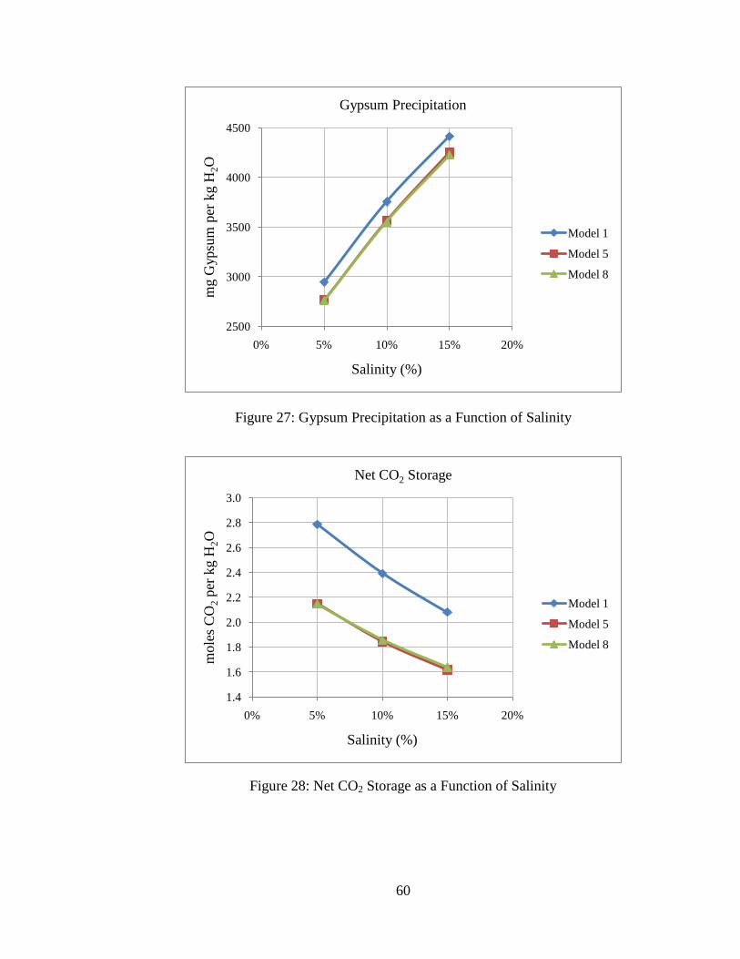
60

Figure 27: Gypsum Precipitation as a Function of Salinity

Figure 28: Net CO2 Storage as a Function of Salinity

2500

3000

3500

4000

4500

0% 5% 10% 15% 20%

mg G

ypsu

m p

er k

g H

2O

Salinity (%)


Model 1

Model 5

Model 8

1.4

1.6

1.8

2.0

2.2

2.4

2.6

2.8

3.0

0% 5% 10% 15% 20%

mole

s C

O2

per

kg H

2O

Salinity (%)

Net CO2 Storage

Model 1

Model 5

Model 8

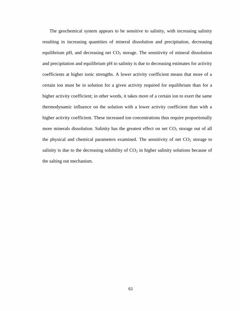
61

The geochemical system appears to be sensitive to salinity, with increasing salinity

resulting in increasing quantities of mineral dissolution and precipitation, decreasing

equilibrium pH, and decreasing net CO2 storage. The sensitivity of mineral dissolution

and precipitation and equilibrium pH to salinity is due to decreasing estimates for activity

coefficients at higher ionic strengths. A lower activity coefficient means that more of a

certain ion must be in solution for a given activity required for equilibrium than for a

higher activity coefficient; in other words, it takes more of a certain ion to exert the same

thermodynamic influence on the solution with a lower activity coefficient than with a

higher activity coefficient. These increased ion concentrations thus require proportionally

more minerals dissolution. Salinity has the greatest effect on net CO2 storage out of all

the physical and chemical parameters examined. The sensitivity of net CO2 storage to

salinity is due to the decreasing solubility of CO2 in higher salinity solutions because of

the salting out mechanism.

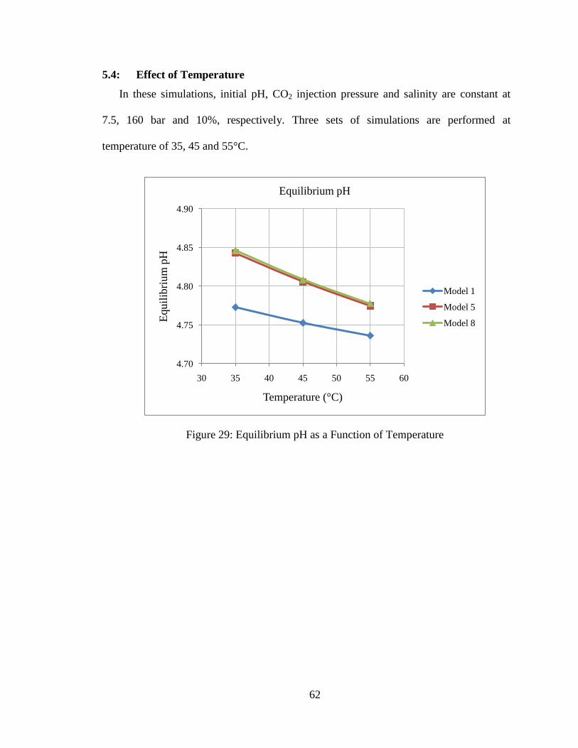
62

5.4: Effect of Temperature

In these simulations, initial pH, CO2 injection pressure and salinity are constant at

7.5, 160 bar and 10%, respectively. Three sets of simulations are performed at

temperature of 35, 45 and 55°C.

Figure 29: Equilibrium pH as a Function of Temperature

4.70

4.75

4.80

4.85

4.90

30 35 40 45 50 55 60

Equil

ibri

um

pH

Temperature (°C)

Equilibrium pH

Model 1

Model 5

Model 8

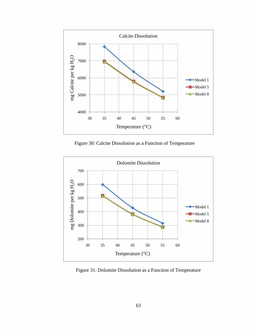
63

Figure 30: Calcite Dissolution as a Function of Temperature

Figure 31: Dolomite Dissolution as a Function of Temperature

4000

5000

6000

7000

8000

30 35 40 45 50 55 60

mg C

alci

te p

er k

g H

2O

Temperature (°C)

Calcite Dissolution

Model 1

Model 5

Model 8

200

300

400

500

600

700

30 35 40 45 50 55 60

mg D

olo

mit

e per

kg H

2O

Temperature (°C)


Model 1

Model 5

Model 8

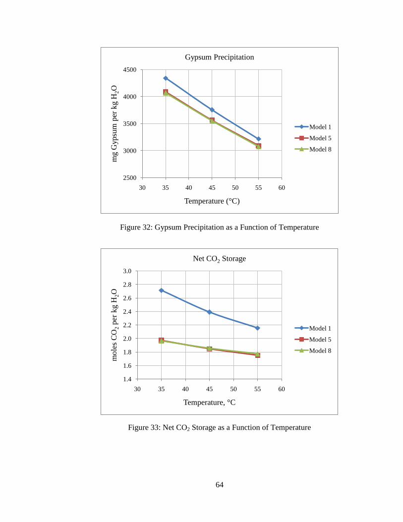
64

Figure 32: Gypsum Precipitation as a Function of Temperature

Figure 33: Net CO2 Storage as a Function of Temperature

2500

3000

3500

4000

4500

30 35 40 45 50 55 60

mg G

ypsu

m p

er k

g H

2O

Temperature (°C)


Model 1

Model 5

Model 8

1.4

1.6

1.8

2.0

2.2

2.4

2.6

2.8

3.0

30 35 40 45 50 55 60

mole

s C

O2

per

kg H

2O

Temperature, °C

Net CO2 Storage

Model 1

Model 5

Model 8

65

The geochemical system appears to be relatively sensitive to temperature, with

increasing temperature resulting in decreasing quantities of mineral dissolution and

precipitation, decreasing equilibrium pH, and decreasing net CO2 storage. Sensitivity to

temperature is due to decreasing equilibrium constants at higher temperatures for the

geochemical reactions considered (see Table 1-Table 4). This effect, known as retrograde

solubility, is particularly pronounced with calcium carbonate (CaCO3(s)). This means that

less free ions must be in solution to achieve equilibrium with the solid mineral phase and

the injected CO2 phase. The decrease in equilibrium pH associated with increased

temperatures is also due to the decreased equilibrium constant for the dissociation of

water. In other words, at elevated temperatures, the activity of H+ ions is increased

relative to standard conditions.

5.5: Effects on Porosity, ε

The formation porosity, ε, is the ratio of void volume to bulk aquifer volume, and can

change as a result of mineral precipitation and dissolution due to CO2 injection. If

significant amounts of minerals dissolve, then porosity will increase. Conversely, if

mineral precipitation is the dominant effect, then porosity will decrease. For simplicity,

geochemical reactions occurring in the brine that is being displaced by the moving CO2

interface are not considered. Rather, only the residual pore brine that is not displaced by

the moving CO2 interface – i.e. it is held in place due to capillary forces – is considered to

reach equilibrium with the CO2 phase. The change in porosity can be estimated as

follows:

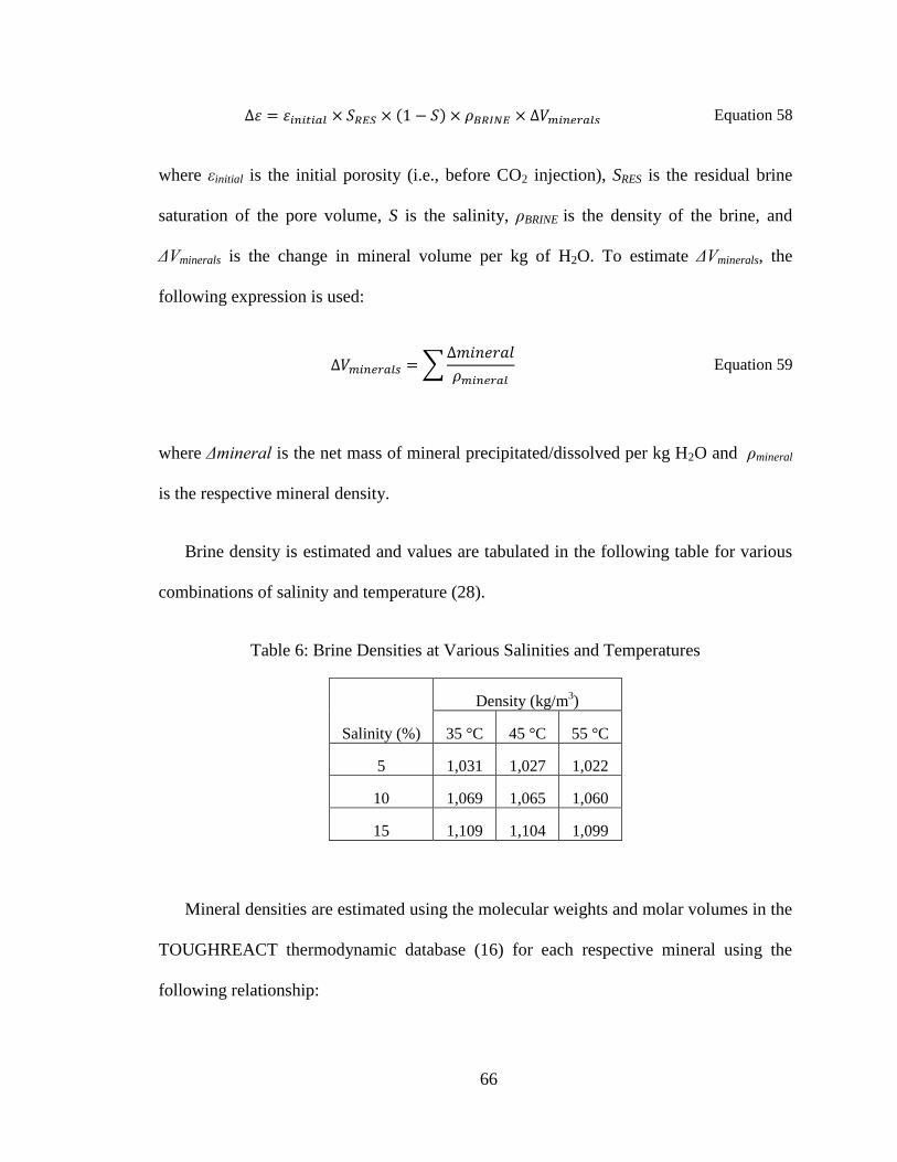
66

Equation 58

where εinitial is the initial porosity (i.e., before CO2 injection), SRES is the residual brine

saturation of the pore volume, S is the salinity, ρBRINE is the density of the brine, and

Δ minerals is the change in mineral volume per kg of H2O. To estimate Δ minerals, the

following expression is used:

Equation 59

where Δmineral is the net mass of mineral precipitated/dissolved per kg H2O and ρmineral

is the respective mineral density.

Brine density is estimated and values are tabulated in the following table for various

combinations of salinity and temperature (28).

Table 6: Brine Densities at Various Salinities and Temperatures

Salinity (%)

Density (kg/m3)

35 °C 45 °C 55 °C

5 1,031 1,027 1,022

10 1,069 1,065 1,060

15 1,109 1,104 1,099

Mineral densities are estimated using the molecular weights and molar volumes in the

TOUGHREACT thermodynamic database (16) for each respective mineral using the

following relationship:

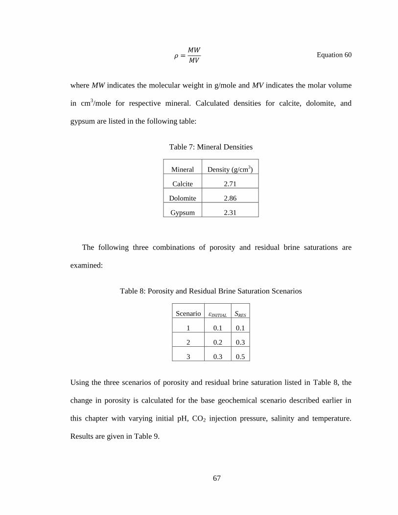
67

Equation 60

where MW indicates the molecular weight in g/mole and MV indicates the molar volume

in cm3/mole for respective mineral. Calculated densities for calcite, dolomite, and

gypsum are listed in the following table:

Table 7: Mineral Densities

Mineral Density (g/cm3)

Calcite 2.71

Dolomite 2.86

Gypsum 2.31

The following three combinations of porosity and residual brine saturations are

examined:

Table 8: Porosity and Residual Brine Saturation Scenarios

Scenario εINITIAL SRES

1 0.1 0.1

2 0.2 0.3

3 0.3 0.5

Using the three scenarios of porosity and residual brine saturation listed in Table 8, the

change in porosity is calculated for the base geochemical scenario described earlier in

this chapter with varying initial pH, CO2 injection pressure, salinity and temperature.

Results are given in Table 9.

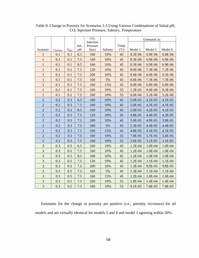
68

Table 9: Change in Porosity for Scenarios 1-3 Using Various Combinations of Initial pH,

CO2 Injection Pressure, Salinity, Temperature

Scenario εINITIAL SRES

Init.

pH

CO2

Injection

Pressure

(bar) Salinity

Temp.

(°C)

Estimated Δε

Model 1 Model 5 Model 8

1 0.1 0.1 6.5 160 10% 45 8.3E-06 6.9E-06 6.8E-06

1 0.1 0.1 7.5 160 10% 45 8.3E-06 6.9E-06 6.9E-06

1 0.1 0.1 8.5 160 10% 45 8.3E-06 6.9E-06 6.9E-06

1 0.1 0.1 7.5 120 10% 45 8.0E-06 7.3E-06 7.2E-06

1 0.1 0.1 7.5 200 10% 45 8.4E-06 6.6E-06 6.5E-06

1 0.1 0.1 7.5 160 5% 45 8.8E-06 7.3E-06 7.3E-06

1 0.1 0.1 7.5 160 15% 45 8.0E-06 6.8E-06 6.8E-06

1 0.1 0.1 7.5 160 10% 35 1.2E-05 9.4E-06 9.3E-06

1 0.1 0.1 7.5 160 10% 55 6.0E-06 5.2E-06 5.2E-06

2 0.2 0.3 6.5 160 10% 45 5.0E-05 4.1E-05 4.1E-05

2 0.2 0.3 7.5 160 10% 45 5.0E-05 4.2E-05 4.1E-05

2 0.2 0.3 8.5 160 10% 45 5.0E-05 4.2E-05 4.1E-05

2 0.2 0.3 7.5 120 10% 45 4.8E-05 4.4E-05 4.3E-05

2 0.2 0.3 7.5 200 10% 45 5.0E-05 4.0E-05 3.9E-05

2 0.2 0.3 7.5 160 5% 45 5.3E-05 4.4E-05 4.4E-05

2 0.2 0.3 7.5 160 15% 45 4.8E-05 4.1E-05 4.1E-05

2 0.2 0.3 7.5 160 10% 35 7.0E-05 5.7E-05 5.6E-05

2 0.2 0.3 7.5 160 10% 55 3.6E-05 3.1E-05 3.1E-05

3 0.3 0.5 6.5 160 10% 45 1.2E-04 1.0E-04 1.0E-04

3 0.3 0.5 7.5 160 10% 45 1.2E-04 1.0E-04 1.0E-04

3 0.3 0.5 8.5 160 10% 45 1.2E-04 1.0E-04 1.0E-04

3 0.3 0.5 7.5 120 10% 45 1.2E-04 1.1E-04 1.1E-04

3 0.3 0.5 7.5 200 10% 45 1.3E-04 9.9E-05 9.8E-05

3 0.3 0.5 7.5 160 5% 45 1.3E-04 1.1E-04 1.1E-04

3 0.3 0.5 7.5 160 15% 45 1.2E-04 1.0E-04 1.0E-04

3 0.3 0.5 7.5 160 10% 35 1.8E-04 1.4E-04 1.4E-04

3 0.3 0.5 7.5 160 10% 55 9.1E-05 7.8E-05 7.8E-05

Estimates for the change in porosity are positive (i.e., porosity increases) for all

models and are virtually identical for models 5 and 8 and model 1 agreeing within 20%.

69

The change in porosity is strongly related to the initial porosity and residual brine

saturation, with estimates spanning three orders of magnitude for initial porosity ranging

from 0.1 to 0.3 and residual brine saturation ranging from 0.1 to 0.5. Specifically, higher

initial porosity and residual brine saturation results in larger estimated changes in

porosity for the geochemical system considered. This is because higher initial porosity

and residual brine saturation implies that there is more brine available per unit aquifer

volume for equilibration with surrounding minerals and the injected CO2, resulting in

larger net mineral dissolution and precipitation quantities per unit aquifer volume.

However, the overall change in porosity is very small for all scenarios considered, with a

maximum change that is three orders of magnitude less than the initial porosity. This

agrees well with observations by others (5; 7).

5.6: Choice of Thermodynamic Sub-model for CO2 Parameter Estimation

In every simulation, model 1 gave the largest net mineral reactions and change in pH.

This is most likely due to the greater fugacity coefficient predicted using the method of

Spycher and Reed (26) and the higher aqueous CO2 concentration predicted using the

equilibrium constant method. Models 5 and 8 use more recently developed correlations

that account for the effects of dissolved salts to estimate the equilibrium dissolved CO2

concentration, and the lower estimated aqueous CO2 concentrations result in slightly

lower net mineral reactions and changes in pH as compared to model 1. However,

estimates of mineral precipitation and dissolution are closely grouped within the same

order of magnitude for all three models, indicating that the choice of thermodynamic sub-

models does not have a significant impact on the estimated quantities.

70

6: Summary and Conclusion

Different thermodynamic sub-models are used to construct overall geochemical

models to describe pre- and post- CO2 injection conditions in a deep, saline aquifer that is

comprised of calcite, dolomite, and gypsum. It is found that the overall geochemical

models are relatively insensitive to appropriate choices for thermodynamic sub-models

for estimating such parameters as CO2(aq) activity coefficient, CO2(g,sc) fugacity

coefficient, and the solubility of CO2(aq). These geochemical models are used to

determine concentrations of ionic species and aqueous complexes and quantify the

amount of minerals that are dissolving into or precipitating out of solution so that the

change in porosity due to CO2 injection can be estimated. All of the models predict that

calcite and dolomite will dissolve and gypsum will precipitate. The models all predict

that CO2 storage by solubility trapping is likely, but carbonate mineral dissolution under

acidic conditions prevents mineral trapping.

It is determined that mineral dissolution and precipitation, along with requisite

changes in porosity, are relatively sensitive to the temperature and salinity of the native

brine in the aquifer and relatively insensitive to the CO2 injection pressure and initial pH

of the brine. However, over the range of conditions examined, the estimated net change

in porosity is low, with a maximum increase of magnitude 10-4

and a minimum increase

of magnitude 10-6

. It appears that CO2 injection and storage in deep, saline aquifers

comprised of calcite, dolomite, and gypsum for the physical and chemical conditions

considered will have little effect on the formation porosity.

71

Works Cited

1. CO2 storage in geological media: Role, means, status and barriers to deployment.

Bachu, Stefan. 2008. Progress in Energy and Combustion Science, Vol. 34, pp. 254-

273.

2. Carbon Dioxide Capture and Storage. Intergovernmental Panel on Climate Change.

Cambridge University Press, 2005.

3. Mineral sequestration of carbon dioxide in a sandstone-shale system. Xu, Tianfu,

Apps, John A and Pruess, Karsten. 2004. Chemical Geology, Vol. 217, pp. 295-318.

4. Numerical modeling of fluid-rock chemical interactions at the supercritical CO2-

liquid interface during CO2 injection into a carbonate reservoir, the Dogger aquifer

(Paris Basin, France). Andre, L, Audigane, P and Menjoz, A. 2007. Energy

Conversion & Management, Vol. 48, pp. 1782-1797.

5. Reactive Transport Modeling of CO2 Sequestration in Deep Saline Aquifers.

Lagneau, V., Pipart, A. and Catalette, H. 2005, Oil & Gas Science and Technology,

Vol. 60, pp. 231-247.

6. CO2 injection into saline carbonate aquifer formations I: laboratory investigation.

Izgec, Omer, Demiral, Birol, Bertin, Henri and Akin, Serhat. 2007. Transport in

Porous Media, Vol. 72, pp. 1-24.

7. Evaluation of Subsurface Sequestration of Carbon Dioxide (CO2) at the Polk Power

Station: Physical and Chemical Modeling. Cunningham, Jeffrey, Stewart, Mark,

Okwen, Roland and Thomas, Mark. 2010. Report to TECO Energy.


Station: Physical and Chemical Modeling Phase III: Detailed Physical Modeling.

Cunningham, Jeffrey, Stewart, Mark and Okwen, Roland. 2008. Report to TECO

Energy.


Station: Physical and Chemical Modeling Phase II: Preliminary Physical Modeling.

Cunningham, Jeffrey, Stewart, Mark and Okwen, Roland. 2007. Report to TECO

Energy.

10. Demonstrating storage of CO2 in geological reservoirs: The Sleipner and SACS

projects. Torp, Tore A and Gale, John. 2004. Energy, Vol. 29, pp. 1361-1369.

72

11. Evaluation of the impact of CO2, co-contaminant gas, aqueous fluid and reservoir

rock interactions on the geologic sequestration of CO2. Knauss, Kevin G, Johnson,

James W and Steefel, Carl I. 2004. Chemical Geology, Vol. 217, pp. 339-350.

12. Numerical modeling of injection and mineral trapping of CO2 with H2S and SO2 in a

sandstone formation. Xu, Tianfu, Apps, John A, Pruess, Karsten and Yamamoto,

Hajime. 2007. Chemical Geology, Vol. 242, pp. 319-346.

13. Pore Scale Modeling of Reactive Transport Involved in Geologic CO2 Sequestration.

Kang, Qinjun, Lichtner, Peter C, Viswanathan, Hari S and Abdel-Fattah, Amr I. 2010.

Transport in Porous Media, Vol. 82.

14. CO2 Injection into Saline Carbonate Aquifer Formations II: Comparison of Numerical

Simulations to Experiments. Izgec, Omer, Demiral, Birol, Bertin, Henri and Serhat,

Akin. 2007. Transport in Porous Media, Vol. 73, pp. 57-74.

15. Sequestration of CO2 in geological media in response to climate change: capacity of

deep saline aquifers to sequester CO2 in solution. Bachu, S. and Adams, J. J. 2003.

Energy Conversion and Management, Vol. 44, pp. 3151-3175

16. TOUGHREACT User's Guide: A simulation Program for Non-isothermal Multiphase

Reactive Ceochemical Transport in Variably Saturated Geologic Media. Xu, Tianfu,

Sonnenthal, Eric, Spycher, Nicolas and Pruess, Karsten. 2004. LBNL-55460

17. Theoretical Prediction of the Thermodynamic Behavior of Aqueous Electrolytes at

High Pressures and Temperatures: IV. Calculation of Activity Coefficients, Osmotic

Coefficients, and Apparent Molal and Standard and Relative Partial Molal Properties

to 600°C. Helgeson, Harold C, Kirkham, David H and Flowers, George C. 1981.

American Journal of Science, Vol. 28, pp. 1249-1516.

18. Theoretical Prediction of the Thermodynamic Behavior of Aqueous Electrolytes at

High Pressures and Temperatures: II. Debye-Huckel Parameters for Activity

Ceofficients and Relative Partial Molal Properties. Helgeson, Harold C and Kirkham,

David H. 1974. American Journal of Science, Vol. 274, pp. 1199-1261.

19. Calculation of multicomponent chemical equilibria and reaction processes in systems

involving minerals, gases and an aqueous phase. Reed, Mark H. 1982. Geochemica et

Cosmochimica Acta, Vol. 46, pp. 513-528.

20. An improved model for the calculation of CO2 solubility in aqueous solutions

containing Na+, K

+, Ca

2+, Mg

2+, Cl

-, and SO4

2-. Duan, Zhenhao, Sun, Rui, Zhu, Chen

and Chou, I-Ming. 2006. Marine Chemistry, Vol. 98, pp. 131-139.

21. CO2-H2O mixtures in the geological sequestration of CO2. II. Partitioning in chloride

brines at 12-100°C and up to 600 bar. Spycher, Nicolas and Pruess, Karsten. 2005.

Geochimica et Cosmochimica Acta, Vol. 69, pp. 3309-3320.

73

22. Boiling and mixing of hydrothermal fluids: Chemical effects on mineral precipitation.

Drummond, J. M. 1981. Ph.D. Thesis, The Pennsylvania State University, University

Park, Pennsylvania.

23. Solubility of Carbon-Dioxide in Aqueous Solutions of Sodium-Chloride -

Experimental Results and Correlation. Rumpf, B, Nicolaisen, H, Ocal, C and Maurer,

G. 1994. Journal of Solution Chemistry, Vol. 23, pp. 431-448.

24. An equation of state for the CH4-CO2-H2O system: I. Pure systems from 0 to 1000°C

and 0 to 8000 bar. Duan, Zhenhao, Moller, Nancy and Weare, John H. 1992.

Geochimica et Cosmochimica Acta, Vol. 56, pp. 2605-2617.

25. An improved model calculating CO2 solubility in pure water and aqueous NaCl

solutions from 273 to 533 K and from 0 to 2000 bar. Duan, Zhenhao and Sun, Rui.

2003. Chemical Geology, Vol. 193, pp. 257-271.

26. Fugacity coefficients of H2, CO2, CH4, H2O and of H2O-CO2-CH4 mixtures: A virial

equation treatment for moderate pressures and temperatures applicable to calculations

of hydrothermal boiling. Spycher, Nicolas F and Reed, Mark H. 1988. Geochimica et


27. CO2-H2O mixtures in the geological sequestration of CO2. I. Assessment and

calculation of mutual solubilities from 12 to 100°C and up to 600 bar. Spycher,

Nicolas, Pruess, Karsten and Ennis-King, Jonathen. 2003. Geochimica et


28. Algorithms for computation of fundamental properties of seawater. Fofonoff, N. P.

and Millard Jr., R. C. UNESCO, 1983.

Documents

Geochemical Modeling of CO2 Sequestration in Dolomitic