Characterization of the Exhaust Flow through the DieselOxidation Catalyst

by

Giffin Symko

A thesis submitted in partial fulfillment of the requirements for the degree of

Master of Science

Department of Mechanical EngineeringUniversity of Alberta

c© Giffin Symko, 2017

ii

Abstract

The result of adding an insulation ring to the interior of the Diesel oxidation

catalyst on pressure drop and light-off characteristics is investigated by injecting a

ceramic material into the channels of the monolith forming a circular ring. The steady

state pressure drop is recorded as a function of the mass flow rate while the transient

temperature response is recorded as a function of time. The experimental results are

compared with a numerical model created using ANSYS Fluent.

The experimental results show no statistical difference in pressure drop with the

addition of an insulation ring as the pulsations in the exhaust flow, created by the

engine, results in uncertainty larger than the expected difference in pressure drop.

The numerical model shows an increase in pressure drop that corresponds to the

decrease in flow area which results in an increase in viscous resistance through the

remaining channels of the monolith.

The experimental results indicate that the addition of an insulation ring increases

the heat capacity of the DOC requiring more energy and time to reach steady state.

However, the numerical model indicates that the increase in time to reach steady

state is due to the slow rate of heating of the insulation ring, while the rate of heating

of the monolith is increased, with the exception of a small area directly adjacent to

the insulation ring.

The experimental results show no statistical difference in pressure drop while

the numerical model indicates an increase in pressure drop with the addition of an

insulation ring. The light-off characteristics of the DOC with the addition of an

insulation ring may be improved as the rate of heating is increased across the monolith,

with the exception of directly adjacent to the insulation ring. Whether the decrease

in the rate of heating adjacent to the insulation ring offsets the benefits of the increase

for the remainder of the monolith needs to be further explored.

iii

Table of Contents

1 Introduction 11.1 Diesel Exhaust Aftertreatment . . . . . . . . . . . . . . . . . . . . . . 11.2 Problem Statement . . . . . . . . . . . . . . . . . . . . . . . . . . . . 21.3 Motivation . . . . . . . . . . . . . . . . . . . . . . . . . . . . . . . . . 21.4 Thesis Organization . . . . . . . . . . . . . . . . . . . . . . . . . . . . 31.5 Contributions . . . . . . . . . . . . . . . . . . . . . . . . . . . . . . . 4

2 Background 52.1 Compression Ignition Engines . . . . . . . . . . . . . . . . . . . . . . 52.2 Exhaust Emissions . . . . . . . . . . . . . . . . . . . . . . . . . . . . 9

2.2.1 Carbon Monoxide . . . . . . . . . . . . . . . . . . . . . . . . . 92.2.2 Oxides of Nitrogen . . . . . . . . . . . . . . . . . . . . . . . . 102.2.3 Hydrocarbons . . . . . . . . . . . . . . . . . . . . . . . . . . . 122.2.4 Particulate Matter . . . . . . . . . . . . . . . . . . . . . . . . 13

2.3 Control of Engine Emissions . . . . . . . . . . . . . . . . . . . . . . . 152.4 Diesel Exhaust Aftertreatment . . . . . . . . . . . . . . . . . . . . . . 15

2.4.1 Diesel Particulate Filter . . . . . . . . . . . . . . . . . . . . . 172.4.2 Selective Catalytic Reduction Catalyst . . . . . . . . . . . . . 182.4.3 Diesel Oxidation Catalyst . . . . . . . . . . . . . . . . . . . . 19

2.5 Catalyst Construction . . . . . . . . . . . . . . . . . . . . . . . . . . 202.5.1 Monolith Geometry . . . . . . . . . . . . . . . . . . . . . . . . 212.5.2 Flow Distribution . . . . . . . . . . . . . . . . . . . . . . . . . 222.5.3 Inlet/Outlet Flow . . . . . . . . . . . . . . . . . . . . . . . . . 222.5.4 Pressure Drop . . . . . . . . . . . . . . . . . . . . . . . . . . . 242.5.5 Monolith Temperature . . . . . . . . . . . . . . . . . . . . . . 27

3 Experimental Setup 293.1 Experimental Setup . . . . . . . . . . . . . . . . . . . . . . . . . . . . 293.2 Engine Specifications . . . . . . . . . . . . . . . . . . . . . . . . . . . 30

3.2.1 Air Intake . . . . . . . . . . . . . . . . . . . . . . . . . . . . . 313.2.2 Air Intake Temperature Control . . . . . . . . . . . . . . . . . 333.2.3 Engine Temperature Control . . . . . . . . . . . . . . . . . . . 33

3.3 Dynamometer . . . . . . . . . . . . . . . . . . . . . . . . . . . . . . . 343.4 Exhaust Setup . . . . . . . . . . . . . . . . . . . . . . . . . . . . . . . 34

iv

3.5 Diesel Oxidation Catalyst . . . . . . . . . . . . . . . . . . . . . . . . 363.6 Sensors . . . . . . . . . . . . . . . . . . . . . . . . . . . . . . . . . . . 373.7 Operating Points . . . . . . . . . . . . . . . . . . . . . . . . . . . . . 403.8 Post Processing and Output Calculations . . . . . . . . . . . . . . . . 41

3.8.1 Intake Air Mass Flow Rate . . . . . . . . . . . . . . . . . . . . 423.8.2 Exhaust Mass Flow Rate . . . . . . . . . . . . . . . . . . . . . 43

3.9 Engine Facility Setup . . . . . . . . . . . . . . . . . . . . . . . . . . . 443.9.1 Ammonia Injection . . . . . . . . . . . . . . . . . . . . . . . . 44

4 Simulation Setup 474.1 Simulation Setup . . . . . . . . . . . . . . . . . . . . . . . . . . . . . 474.2 Geometry and Meshing . . . . . . . . . . . . . . . . . . . . . . . . . . 48

4.2.1 Material Properties . . . . . . . . . . . . . . . . . . . . . . . . 494.3 Heat Transfer . . . . . . . . . . . . . . . . . . . . . . . . . . . . . . . 504.4 Turbulence . . . . . . . . . . . . . . . . . . . . . . . . . . . . . . . . . 514.5 Porous Zone . . . . . . . . . . . . . . . . . . . . . . . . . . . . . . . . 524.6 Viscous Resistance Factors . . . . . . . . . . . . . . . . . . . . . . . . 534.7 Mesh Dependency . . . . . . . . . . . . . . . . . . . . . . . . . . . . . 56

5 Experimental Flow Characterization 575.1 Steady State Pressure Drop . . . . . . . . . . . . . . . . . . . . . . . 575.2 Steady State Temperature Profile . . . . . . . . . . . . . . . . . . . . 595.3 Transient Temperature Profile . . . . . . . . . . . . . . . . . . . . . . 635.4 DOC Energy Absorption . . . . . . . . . . . . . . . . . . . . . . . . . 685.5 Experimental Limitations . . . . . . . . . . . . . . . . . . . . . . . . 76

6 Simulation Based Flow Characterization 776.1 Steady State Numerical Model . . . . . . . . . . . . . . . . . . . . . . 77

6.1.1 Steady State Setup . . . . . . . . . . . . . . . . . . . . . . . . 776.1.2 Mass Flow Profile . . . . . . . . . . . . . . . . . . . . . . . . . 786.1.3 Pressure Drop . . . . . . . . . . . . . . . . . . . . . . . . . . . 796.1.4 Steady State Temperature Profile . . . . . . . . . . . . . . . . 80

6.2 Transient Numerical Model . . . . . . . . . . . . . . . . . . . . . . . 836.2.1 Temperature Input . . . . . . . . . . . . . . . . . . . . . . . . 836.2.2 Transient Model Validation . . . . . . . . . . . . . . . . . . . 846.2.3 DOC Heating Characteristics . . . . . . . . . . . . . . . . . . 88

6.3 Assumptions and Limitations . . . . . . . . . . . . . . . . . . . . . . 90

7 Conclusions 927.1 Pressure Drop . . . . . . . . . . . . . . . . . . . . . . . . . . . . . . . 927.2 Temperature Profile . . . . . . . . . . . . . . . . . . . . . . . . . . . . 937.3 Insulation Ring . . . . . . . . . . . . . . . . . . . . . . . . . . . . . . 947.4 Future Work . . . . . . . . . . . . . . . . . . . . . . . . . . . . . . . . 95

References 96

v

A CFD Background 105A.1 Turbulent Flow . . . . . . . . . . . . . . . . . . . . . . . . . . . . . . 105

A.1.1 Production of Turbulent Kinetic Energy, Gk . . . . . . . . . . 108A.1.2 Production of Specific Dissipation Rate, Gω . . . . . . . . . . 108A.1.3 Dissipation of Turbulent Kinetic Energy, Yk . . . . . . . . . . 109A.1.4 Dissipation of Specific Dissipation Rate, Yω . . . . . . . . . . . 110A.1.5 Compressibility Function, F (Mt) . . . . . . . . . . . . . . . . 111A.1.6 Cross-Diffusion, Dω . . . . . . . . . . . . . . . . . . . . . . . . 112

A.2 Porous Flow . . . . . . . . . . . . . . . . . . . . . . . . . . . . . . . . 112A.3 Heat Transfer . . . . . . . . . . . . . . . . . . . . . . . . . . . . . . . 113

B Uncertainty 115B.1 Theory . . . . . . . . . . . . . . . . . . . . . . . . . . . . . . . . . . . 115

vi

List of Tables

3.1 Engine Specifications . . . . . . . . . . . . . . . . . . . . . . . . . . . 313.2 Inside and outside diameters of monolith insulation rings . . . . . . . 373.3 Radial location of thermocouples in monolith . . . . . . . . . . . . . . 393.4 Experimental operating points (± is based on maximum deviation) . 42

4.1 Dimensions of DOC as illustrated in Figures 4.1 and 4.2 . . . . . . . 484.2 Mesh sizing by component . . . . . . . . . . . . . . . . . . . . . . . . 504.3 DOC material properties . . . . . . . . . . . . . . . . . . . . . . . . . 514.4 SST k-omega turbulent flow parameters . . . . . . . . . . . . . . . . . 51

5.1 List of thermocouples located next to the insulation ring . . . . . . . 665.2 Coefficients used to calculate Cp(T ) . . . . . . . . . . . . . . . . . . . 69

vii

List of Figures

2.1 Relationship between compression ratio and theoretical engine efficiency 72.2 P-V diagram of a 4-stroke mechanical Diesel cycle . . . . . . . . . . . 82.3 Exhaust aftertreatment schematic for a 6.7L Ford F-150 Diesel pickup 162.4 DOC showing the interior honeycomb like structure . . . . . . . . . . 212.5 Schematic of the components that make up the DOC (axisymmetric) 222.6 Positioning of the insulation ring inside the monolith of the DOC . . 24

3.1 Exhaust bypass setup . . . . . . . . . . . . . . . . . . . . . . . . . . . 303.2 Schematic of the experimental setup . . . . . . . . . . . . . . . . . . 303.3 Cummins 4-cylinder QSB4.5 (Tier 3) Diesel Engine . . . . . . . . . . 313.4 Custom air intake with HFM sensor . . . . . . . . . . . . . . . . . . . 323.5 Air intake temperature control system . . . . . . . . . . . . . . . . . 333.6 CB100-24L flat plate heat exchanger . . . . . . . . . . . . . . . . . . 343.7 Dyne Systems 1014 W Torque/Power Curves . . . . . . . . . . . . . . 353.8 DOC dimensions with monolith represented by the shaded area . . . 363.9 Structure of the DOC (shown in cross section) . . . . . . . . . . . . . 373.10 ECM sensors for NOx, NH3, and %O2 . . . . . . . . . . . . . . . . . . 383.11 INLINE 6 Data Link Adapter from Cummins . . . . . . . . . . . . . 383.12 Locations of thermocouples in the monolith (shown in cross section) . 393.13 Exhaust setup showing the sensors and data acquisition equipment . 403.14 DAQ Box used for the thermocouples and pressure sensor . . . . . . . 413.15 Comparison of engine fuel and air consumption . . . . . . . . . . . . 453.16 Schematic of the ammonia injection system . . . . . . . . . . . . . . . 463.17 Ammonia concentration in the exhaust stream . . . . . . . . . . . . . 46

4.1 Axisymmetric model used for numerical model of DOC . . . . . . . . 484.2 Detailed geometry of porous zone (see Figure 4.1) . . . . . . . . . . . 494.3 DOC meshing using ANSYS ICEM to create structured mesh . . . . 504.4 Trend used to calculate the inertial and viscous resistance factors . . 534.5 Trend used to calculate the viscous resistance factor . . . . . . . . . . 554.6 Mesh dependency results showing convergence of the solution . . . . . 56

5.1 Pressure drop for each of the four DOCs connected to the Diesel engine 585.2 Cold flow pressure drop results for each of the four DOCs . . . . . . . 595.3 Radial temperature profile of the downstream side of the DOC monolith 615.4 Maximum DOC temperature at steady state . . . . . . . . . . . . . . 62

viii

5.5 Radial temperature profile of monolith at 1500 rpm and 50 ft-lbs (68 Nm) 655.6 Radial temperature profile of DOC during heat up for 50 seconds . . 685.7 Energy absorption of the four DOCs . . . . . . . . . . . . . . . . . . 715.8 Energy absorbed by DOC from cold start to steady state . . . . . . . 725.9 Comparison of the heat up time of the DOC . . . . . . . . . . . . . . 75

6.1 Velocity profile of exhaust gases passing through the monolith . . . . 796.2 Pressure drop across the DOC for each of the DOC configurations . . 806.3 Radial temperature profile of the downstream side of the DOC monolith 826.4 Monolith temperature profile for each of the four DOC configurations 836.5 Inlet temperature of the exhaust gas used in the numerical analysis . 846.6 Heating characteristics of the DOC monolith . . . . . . . . . . . . . . 876.7 Comparison of the heating characteristics of the four DOC configurations 90

ix

Nomenclature

Acronyms

BDC Bottom Dead Centre

BSFC Brake Specific Fuel Consumption

CI Compression Ignition

CPSI Cells per Square Inch

DEF Diesel Exhaust Fluid

DNS Direct Numerical Simulation

DOC Diesel Oxidation Catalyst

DPF Diesel Particulate Filter

EGR Exhaust Gas Recirculation

EPA Environmental Protection Agency

GHG Greenhouse Gas

HC Hydrocarbons

HCCI Homogeneous Charge Compression Ignition

HFM Hot Film Mass

IC Internal Combustion

LES Large Eddy Simulation

LNT Lean NOx Trap

MAF Mass Air Flow

NHTSA National Highway Traffic Safety Administration

x

NOx Oxides of Nitrogen

PID Proportional Integral Derivative

PM Particulate Matter

PPCI Partially Premixed Compression Ignition

R Universal Gas Constant

RANS Reynolds Averaged Navier-Stokes

SCR Selective Catalytic Reduction

SI Spark Ignition

SST Shear-Stress Transport

TDC Top Dead Centre

xi

Symbols

α Permeability (1/α is the Viscous Resistance Factor)

α Cut-Off Ratio

δ Kroneker delta

∆P Differential pressure

ε Porosity

η Engine Efficiency

γ Ratio of Gas Specific Heats

µ Dynamic Viscosity

µT Dynamic Turbulent Viscosity

ρ Density

ω Specific Dissipation Rate

A Cross-Sectional Area

CP (T ) Temperature dependent specific heat capacity

C0 Discharge Coefficient

C2 Inertial Resistance Factor

Dc Hydraulic Diameter

dm Mean Particle Diameter

hv Energy associated with Sunlight

E Energy

EA Activation Energy

f Frequency

Gω Generation of Turbulent Kinetic Energy

Gk Generation of Specific Dissipation Rate

k Turbulence Kinetic Energy

xii

kT Reynolds Stress Tensor

k+ Forward Reaction Rate Constant

k- Backward Reaction Rate Constant

keff Effective Thermal Conductivity

kf Fluid Thermal Conductivity

ksf Solid Thermal Conductivity

L Length

m Mass Flow Rate

P Pressure

Q Volumetric Flow Rate

r Radius

Re Reynolds Number

rv Compression Ratio

~S Porous Zone Source Term

S User-Defined Source Term

Sω User-Defined Source of Turbulent Kinetic Energy

Sk User-Defined Source of Specific Dissipation Rate

t Time

T Temperature

u Velocity

v Kinematic Viscosity

vT Turbulent Kinematic Viscosity

Vout Output Voltage

Wpower Work produced

Wpump Pumping work

Y Molar Concentration

Yω Dissipation of Turbulent Kinetic Energy

Yk Dissipation of Specific Dissipation Rate

1

Chapter 1

Introduction

This Chapter details the problem addressed in this thesis, why it should be addressed,

and how it is investigated.

1.1 Diesel Exhaust Aftertreatment

Since the 1970s, legislation governing the emissions from automobiles has become

increasing stringent which has required auto manufacturers to rely on advances in

aftertreatment systems to ensure compliance. Advances in combustion control strate-

gies, such as exhaust gas recirculation and injection timing, have become insufficient

at reducing tailpipe emissions to meet legislated levels of emissions, this has required

auto manufacturers to rely on advances in aftertreatment devices, such as catalysts

and filters, to ensure compliance of tailpipe emissions.

Aftertreatment systems for Diesel engines are often composed of two catalysts, the

Diesel Oxidation Catalyst (DOC) and Selective Catalytic Reduction Catalyst (SCR),

used to oxidize hydrocarbons (HC) and reduce oxides of nitrogen (NOx). The addition

of a Diesel Particulate Filter (DPF) is used in conjunction with the catalysts to remove

particulate matter (PM) from the exhaust. The addition of each component reduces

regulated emissions such as HC, NOx, and PM but increases the back pressure on the

engine reducing the efficiency of the engine and leading to increased fuel consumption

2

and increased CO2 tailpipe emissions.

1.2 Problem Statement

The objective of this research is to characterize the flow of exhaust gas through the

DOC. To understand the flow through the DOC and its effect on the DOC, a number

of key aspects are observed including the pressure drop, the heating characteristics

affecting the light-off temperature, and the effect of altering the internal geometry.

The experimental results are compared to numerical simulations for a greater under-

standing of the internal flows inside the monolith and to aid in developing a numerical

model of the DOC for future work.

1.3 Motivation

Governments worldwide are acting to decrease harmful emissions and decrease the

amount of CO2 produced by automotive engines, requiring manufacturers to both op-

timize current systems to minimize the emissions produced and to develop new meth-

ods of eliminating emissions produced by the engine. The Environmental Protection

Agency (EPA) and the National Highway Traffic Safety Administration (NHTSA)

have issued rules to reduce greenhouse gases (GHG) emissions for model year vehicles

2017-2025. The EPA regulations are expected to result in an average combined pro-

duction of no more than 101.28 g/km (163 g/mile) of CO2, equivalent to an average

fuel consumption of 4.32 L/100 km (54.5 mpg) by the end of 2025 [EPA, 2012].

Over the last several years, efforts to achieve high efficiency combustion engines

while simultaneously reducing exhaust emissions using low temperature combustion

have been made. One way to do this is by taking a spark ignition (SI) engine and pro-

ducing a homogeneous charge that autoignites [Yao et al., 2009] and usually requires

control [Ghazimirsaied and Koch, 2012; Strandh et al., 2004; Ebrahimi and Koch,

3

2015]. Mazda is now implementing this technology into their production automobiles

[Mazda, 2017]. Another way to achieve high efficiency and low emissions is by taking

a Diesel engine and using a partially premixed charge [Manente et al., 2011]. The

advances in engine technology, particularly the use of low temperature combustion,

will require corresponding advances in exhaust aftertreatment technology.

By characterizing the flow through the DOC, the DOC construction can be op-

timized to minimize the pressure drop and improve the light-off characteristics. By

decreasing the pressure drop, the back pressure on the engine is reduced improving

the overall efficiency and leading to a decrease in fuel consumption. Improved light-off

characteristics can lead to a significant reduction in tailpipe emissions, as it has been

found that as much as 50% to 80% of emissions are produced during cold start prior

to the catalyst reaching light-off temperature [Hadavi et al., 2013; Shen et al., 1999;

Cho et al., 1998].

Finally, by characterizing the flow through the DOC, the results can be used to

validate the numerical models. These models will provide a greater understanding of

the flow characteristics and will allow for better optimization of the DOC by man-

ufacturers and provide more efficient control of the system by the engine controller.

As it is expected that auto manufacturers will meet emissions regulations through

improvements in engine control and aftertreatment systems [EPA, 2012], the ability

to optimize these systems is crucial to meeting regulations.

1.4 Thesis Organization

The thesis begins with the experimental results used to characterize the flow of ex-

haust across the DOC both with and without the addition of insulation rings in the

monolith. This includes the overall pressure drop and radial temperature profile at

steady state and during heating and cooling of the DOC.

4

The results from the numerical analysis are compared against the experimental

results to determine the validity of the numerical model. The numerical model is

used to determine the effect of adding an insulation ring to the monolith and to

help validate the experimental results. The experimental and numerical results are

compared for steady state and transient tests to determine whether any conclusions

can be drawn and show the insulating ring exibits marginal improvements. The

benefits or drawbacks of adding an insulation ring to the monolith are examined in

detail.

1.5 Contributions

The major contributions of this study are:

• Characterizing the flow of exhaust gas through the DOC, including the pressure

drop and temperature profile for various DOC configurations.

• Developing a simple 2D axisymmetric numerical model for optimizing the con-

struction of the DOC.

• Creating a Diesel engine exhaust setup with sensors and analysis software. The

engine and exhaust aftertreatment setup will be an excellent testing facility for

future aftertreatment studies.

5

Chapter 2

Background

An overview of the topics of this thesis are discussed in the context of research in the

literature.

2.1 Compression Ignition Engines

Compression ignition (CI) engines are attractive due to their higher efficiency in

comparison to spark ignition (SI) engines, leading to reduced CO2 production and

fuel consumption. Despite the benefits, CI engines produce emissions that are difficult

to reduce and often in quantities much greater than SI engines, including oxides of

nitrogen, particulate matter, and hydrocarbons. Various strategies are employed to

reduce these emissions but most increase the complexity of the system and reduce

the overall efficiency.

Power in a modern CI engine is produced by drawing air into the cylinder and

then compressing it, increasing the air temperature above the ignition temperature of

the fuel. The fuel is then injected and ignites, further increasing the cylinder pressure

and pushing the piston downward. During fuel injection, mass transfer causes the

air and fuel to mix by means of diffusion and turbulence. During mixing, the fuel

combusts at the interface where the mixture reaches an equivalence ratio that is

within combustible limits.

6

CI engines are capable of much higher compression ratios as the charge is not

premixed prior to compression and are therefore not subject to the same constraints

as SI engines, where the charge is premixed. The theoretical engine efficiency for SI,

ηSI, and CI, ηCI, engines are given by,

ηSI = 1− 1

rvγ−1

(2.1)

ηCI = 1− 1

rvγ−1

[αγ − 1

γ(α− 1)

](2.2)

where rv is the compression ratio, α is the cut-off ratio, and γ is the ratio of gas specific

heats [Stone, 2012]. Comparing Equations 2.1 and 2.2, for the same compression ratio,

SI engines will have a higher efficiency due to the factor in square brackets in Equation

2.2 since the cut-off ratio, α, will always fall within the range 1 < α < rv, making

the term in square brackets always greater than one [Stone, 2012]. However, since CI

engines are capable of operating at much higher compression ratios, they are typically

more efficient than SI engines. This makes CI engines attractive as increased engine

efficiency leads to lower CO2 production and fuel consumption.

The main drawback of CI engines is related to the mode of combustion occuring

in the cylinder. Unlike SI engines where the charge is premixed, in CI engines the

charge is injected into the cylinder after the air in the cylinder has been compressed

and the ignition temperature of the fuel has been exceeded. During injection a com-

bustion interface between the air and fuel occurs since the time dependency of mass

transfer limits the flame to an interface where blending results in a local equivalence

ratio sufficient for combustion, with the primary mechanisms of mass transfer being

diffusion and turbulence. The time dependency of mass transfer limits the maximum

engine speed and is the cause for many of the emissions produced by CI engines.

7

Because the diffusion flame is locally rich and lean, it produces emissions associated

with both, along with particulate matter and hydrocarbons [Shum-Kivan et al., 2016].

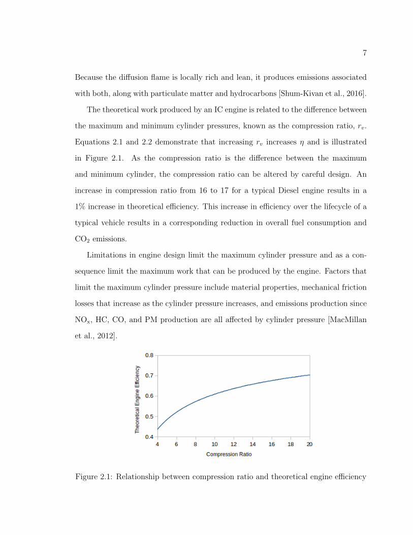
The theoretical work produced by an IC engine is related to the difference between

the maximum and minimum cylinder pressures, known as the compression ratio, rv.

Equations 2.1 and 2.2 demonstrate that increasing rv increases η and is illustrated

in Figure 2.1. As the compression ratio is the difference between the maximum

and minimum cylinder, the compression ratio can be altered by careful design. An

increase in compression ratio from 16 to 17 for a typical Diesel engine results in a

1% increase in theoretical efficiency. This increase in efficiency over the lifecycle of a

typical vehicle results in a corresponding reduction in overall fuel consumption and

CO2 emissions.

Limitations in engine design limit the maximum cylinder pressure and as a con-

sequence limit the maximum work that can be produced by the engine. Factors that

limit the maximum cylinder pressure include material properties, mechanical friction

losses that increase as the cylinder pressure increases, and emissions production since

NOx, HC, CO, and PM production are all affected by cylinder pressure [MacMillan

et al., 2012].

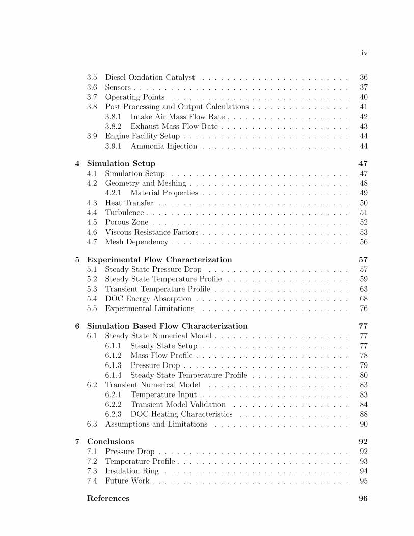
Figure 2.1: Relationship between compression ratio and theoretical engine efficiency

8

The minimum cylinder pressure is directly related to the downstream pressure

drop from the engine to tailpipe. With the addition of catalysts and filters, the back

pressure on the engine is increased. Figure 2.2 shows a 4-stroke mechanical Diesel

cycle with the maximum cylinder pressure shown as Pmax, the engine out pressure as

P0, the area containing Wpower is the power produced by the compression/expansion

stroke, while the area containing Wpump is the pumping work required during the

exhaust/intake stroke.

Figure 2.2: P-V diagram of a 4-stroke mechanical Diesel cycle

The addition of aftertreatment devices increases P0 and reduces Wpower by decreas-

ing the compression ratio, rv, calculated by Pmax−P0, causing the area in Figure 2.2

containing Wpower to be reduced. Furthermore, the addition of aftertreatment devices

increases Wpump reducing the overall power output of the engine, Wpower−Wpump. By

minimizing the pressure drop between the engine and the tailpipe, the overall power

output of the engine can be increased, increasing the overall engine efficiency.

9

2.2 Exhaust Emissions

The stoichiometric combustion of any hydrocarbon produces CO2 and H2O by the

following reaction,

CxHy + (x+y

2)O2 → xCO2 +

y

2H2O (2.3)

however the actual combustion of hydrocarbons in IC engines produce other com-

pounds that are harmful to the environment and health as well as reduce the overall

efficiency of the engine. Of particular interest are carbon monoxide (CO), particulate

matter (PM), hydrocarbons (HC), and oxides of nitrogen (NOx). Because of their

negative effects, stringent government regulations are in place to limit the tailpipe

emission gases produced by IC engines.

2.2.1 Carbon Monoxide

In IC engines, CO is produced primarily during rich combustion when insufficient

oxygen is available for complete oxidation of the fuel. In CI engines which operate

under lean conditions, the amount of CO produced is minimal and the primary source

occurs when the local temperature is insufficient and the rates of reaction are too slow

for oxidation to occur. This occurs in regions where the local temperature is unable

to achieve high combustion temperatures, such as next to the cylinder walls which

act as a heat sink [Barbosa, 2016]. CO production is an intermediate step in the

production of CO2 from a hydrocarbon and is given by,

RH→ R→ RO2 → RCHO→ RCO→ CO (2.4)

10

where R is the hydrocarbon radical [Valerio et al., 2003; Heywood et al., 1988]. CO

is then oxidized through the following reactions,

CO + OHk+1�k−1

CO2 + H (2.5)

CO2 + Ok+2�k−2

CO + O2 (2.6)

where k is the rate constant with the + or - indicating the forward and backwards

reaction direction, respectively [Valerio et al., 2003]. The rate constants can be found

using the Arrnhenius equation, given by,

k = Ae−EARcT (2.7)

where A is a reaction specific constant, E A is the activation energy, Rc is the univer-

sial gas constant, and T is the temperature. Equation 2.7 demonstrates the strong

temperature dependence of Equations 2.5 and 2.6. At low temperatures the rates of

reaction become negligible not allowing the reaction to progress and equilibrium to

be achieved, this results in incomplete oxidation and the production of CO from the

engine.

2.2.2 Oxides of Nitrogen

NOx is produced at high temperatures during lean combustion when excess oxygen is

available, increasing exponentially with temperature [Barbosa, 2016]. NOx are toxic

gases with adverse respiratory effects [WHO, 2006] and leads to the formation of smog

in the atmosphere [Carpenter et al., 1998; Muilwijk et al., 2016]. Smog is produced

11

by photolysis of NO2 in the presence of sunlight (hv) through the following reactions

[Heywood et al., 1988; Carpenter et al., 1998; Barbosa, 2016],

NO2hv−→ NO + O (2.8)

O + O2 −→ O3 (2.9)

leading to the production of the ozone (O3), which is responsible for the formation of

smog.

The kinetic mechanisms by which NOx is produced include [Barbosa, 2016],

1. thermal NOx (also known as the extended Zeldovich mechanism)

2. prompt NOx (also known as the Fenimore mechanism)

3. fuel NOx

The first two mechanisms convert atmospheric nitrogen to NOx while the last converts

fuel based nitrogen to NOx. The primary mechanism of NOx production in IC engines

is thermal NOx, by which over 90% of all NOx emissions are produced [Barbosa, 2016;

Hernandez et al., 2007]. Thermal NOx is produced by the following three reactions

[Bowman, 1975; Merryman and Levy, 1975],

O + N2 � NO + N (2.10)

N + O2 � NO + O (2.11)

N + OH � NO + H (2.12)

12

The rates of reaction are strongly temperature dependent, with temperatures

greater than 2200 K required for reactions to proceed [Barbosa, 2016]. At high tem-

peratures, production is favoured while at low temperatures the reverse reactions are

favoured. Since the rates of reaction are too small for the reaction to proceed at

low temperatures the NO produced during cylinder peak temperatures remain as the

temperature drops during the expansion stroke.

The (NO2)/(NO) ratio produced in IC engines is typically very small [Bowman,

1975], however some studies have shown that NO2 can account for up to 30% of

the NOx emissions [Hilliard and Wheeler, 1979]. Despite NO being formed in much

greater quantities than NO2, NO is oxidised at low temperatures to NO2 resulting

in nearly all NO emissions being converted to NO2 in the environment after being

exhausted [Stone, 2012].

2.2.3 Hydrocarbons

Hydrocarbons (HC) are the result of the incomplete combustion of fuel. It has been

found that many of the HC found in the exhaust are not present in the fuel, which

indicates that the fuel undergoes cracking and synthesis occuring during the high

cylinder temperatures during compression and combustion [Bowman, 1975]. Not all

HC emissions are harmful since some are inert, however, some of the HC emissions

lead to photochemical reactions causing smog, others are potent greenhouse gases

(methane), while others are directly toxic to human health [Pachauri et al., 2014;

Andrews et al., 2007; Bowman, 1975].

HC emissions from IC engines are often produced during rich combustion where

all of the fuel fails to combust, but since CI engines operate lean, HC emissions tend

to be minimal [Barbosa, 2016]. HC emissions from CI engines tend to be the result

of three sources [Heywood et al., 1988]:

13

• undermixing

• quenching

• absorption/desorption.

HC emissions from undermixing occur when the fuel inadequately mixes during in-

jection resulting in locally rich regions where the fuel fails to mix during combustion.

One main source of undermixing is the result of fuel remaining in the injector nozzle

sac and vaporizing after the cylinder pressure drops and the exhaust valve opens. HC

emissions from quenching occur when fuel reaches areas where the temperature is

insufficient for combustion and the flame is quenched. HC emissions from quenching

occur along the cylinder walls or between the cylinder and piston where the space

is too small for the flame to propagate [Bowman, 1975]. Finally, emissions from ab-

sorption/desorption occur as a result of hydrocarbons absorbing into the engine oil

at high pressure when the piston is near top dead centre (TDC) and desorbing as the

pressure drops and the piston nears bottom dead centre (BDC).

2.2.4 Particulate Matter

From Diesel engines, PM is composed primarily of carbanaceous material with at-

tached organic molecules, known as black carbon [Bond et al., 2013; Heywood et al.,

1988]. PM has been linked to an increased risk of cardiopulmonary mortality and

long term chronic health problems [Pope III and Dockery, 2006; WHO et al., 2012].

It has been found that even increases as small as 50 µg/m3 were found to increase

mortality by 2% to 4% [Kunzli et al., 2000; Katsouyanni et al., 1997]. Furthermore,

the effect of black carbon on climate change is significant as it absorbs more sunlight

than it reflects, leading to increased atmospheric temperatures [Bond et al., 2013].

PM is the result of incomplete combustion in locally rich areas where insufficient

oxygen is available. Particulate matter varies in composition containing 50% to 90%

14

carbon along with other components including oxygen, sulphur, phosphorous, iron,

calcium, and zinc, depending on availability during PM formation [Clague et al.,

1999].

The formation of PM is a two step process; nucleation and agglomeration [Dhal

et al., 2017]. Nucleation occurs with the formation of an aromatic ring structure at

high temperature, as the hydrogen bonds are broken, leaving carbon chains. The

carbon chains then undergo polycyclic aromatic ring growth which results in particle

nucleation [Dhal et al., 2017; Heywood et al., 1988]. The particles then grow primar-

ily by surface growth involving the attachment of available gas phase particles and

through agglomeration where individual soot particles collide [Dhal et al., 2017].

Once PM enters into the atmostphere, Leung et al. [2017] have shown its growth

to occur in three phases. In the first phase the density of the particles increases due to

surface growth of secondary organic aerosols while the shape of the black carbon/soot

remains unchanged. The second stage involves soot restructuring while surface growth

of the particle continues with the addition of secondary organic aerosols. The third

stage involves continued growth of the particle while the shape of the particle tends

towards becoming spherical [Leung et al., 2017]. The coating on the particle continues

to grow while the shape of the particle continues to restructure until the particle

becomes nearly spherical with a shape factor approaching one [Ghazi and Olfert,

2013].

Coating black carbon with organic components has an important effect on climate

forcing, increasing the radiative absorption of black carbon by up to a factor of 2

[Cappa et al., 2012]. The increase in radiative absorption is a result of the organic

coating refracting sunlight towards the black carbon core, increasing the effective

absorptive area of the particle [Bond and Bergstrom, 2006] and increasing the energy

absorbed.

15

2.3 Control of Engine Emissions

Control of tailpipe emissions from Diesel engines is difficult and involves numerous

strategies and additional equipment. Strategies can be divided into two broad cat-

egories; combustion control strategies and exhaust aftertreatment strategies. Com-

bustion control strategies involve limiting the cylinder conditions that result in the

production of emissions, for example, controlling injection timing, rate of fuel in-

jection, and exhaust gas recirculation (EGR) [Barbosa, 2016]. A number of low

temperature combustion strategies exist that attempt to reduce the cylinder pressure

and temperature to minimize emission production and include homogeneous charge

compression ignition (HCCI) [Price et al., 2007] and partially premixed compression

ignition (PPCI) [Noehre et al., 2006]. However, decreasing one emission often results

in an inadvertent increase in another, resulting in a tradeoff between two emissions

[Barbosa, 2016]. For example, EGR decreases NOx emissions by reducing the peak

cylinder temperature but also causes an increase in PM due to the decrease in avail-

able oxygen and decrease in temperature.

To meet emission regulations, combustion control strategies need ultimately be

combined with exhaust aftertreatment strategies. Aftertreatment strategies include

the use of catalysts and filters to reduce or eliminate specific components in the

exhaust. The drawback of using aftertreatment strategies is the increase in back

pressure on the engine which results in a decrease in engine efficiency and increase in

fuel consumption.

2.4 Diesel Exhaust Aftertreatment

The typical CI engine relies on multiple catalysts and a filter to reduce engine-out

emissions to meet tailpipe emission regulations. This is unlike SI engines which are

capable of meeting tailpipe emissions regulations with the use of a single three-way

16

catalyst. A typical exhaust setup for a CI engine will include a Diesel Oxidation

Catalyst (DOC) to reduce HC emissions, Selective Catalytic Reduction (SCR) cata-

lyst or Lean NOx Trap (LNT) to reduce NOx emissions, and Diesel Particulate Filter

(DPF) to reduce PM emissions. Figure 2.3 is the schematic for a 2015 6.7L Ford

F-150 Diesel pickup and is representative of the aftertreatment system used on the

majority of vehicles with a CI engine [Ford Motor Company, 2014].

Figure 2.3: Exhaust aftertreatment schematic for a 6.7L Ford F-150 Diesel pickup

Catalysts and filters are complex, expensive, and require multiple sensors for mon-

itoring and control. In addition to the increased cost and complexity, the addition

of aftertreatment systems increases the overall pressure drop from engine to tailpipe

and leads to an increase in back pressure on the engine. An increase in back pressure

leads directly to a reduction in engine efficiency, an increase in fuel consumption, and

an increase in CO2 production.

17

2.4.1 Diesel Particulate Filter

One of the greatest challenges in the design of IC engines is effectively reducing PM

to meet emissions regulations. Engine control strategies have become insufficient at

reducing PM making aftertreatment strategies necessary. The addition of a DPF

to the aftertreatment system is an effective way of reducing tailpipe PM emissions,

however, the addition of a filter to the exhaust system increases the back pressure on

the engine.

The DPF is designed to trap up to micrometre sized particles and increase the

reactivity of these particles during DPF regeneration [Konstandopoulos et al., 2000].

Regeneration of the DPF can be accomplished via one of three primary methods; pas-

sive regeneration, active regeneration, and mixed passive-active regeneration [Chen

et al., 2014].

Passive regeneration uses a catalyst coated DPF where PM matter is oxidized on

the surface of the catalyst with NO2 [Kotrba et al., 2013]. The advantages of the

passive regeneration system are that it requires lower exhaust temperatures and is

independent of the engine functioning, thereby not requiring a complicated control

strategy. The disadvantages of the system are that it requires a catalyst coating and

a specific exhaust NO2/NOx ratio, requiring an upstream catalyst such as a DOC to

ensure a proper ratio [Kotrba et al., 2013].

Active regeneration requires high exhaust temperatures (> 550◦C) so that PM

oxidation occurs with oxygen available in the exhaust [Chen et al., 2014]. Because

Diesel engine exhaust temperatures rarely achieve the required temperature, various

strategies need to employed to increase the exhaust temperature. Strategies include

locating the DOC directly upstream of the DPF and increasing the HC in the exhaust,

either by direct injection or late post-injection in the cylinder, and having them oxidise

in the DOC, which creates heat that is transferred to the DPF for regeneration [Chen

18

et al., 2014].

Mixed passive-active DPF regeneration is a blend of both the passive and active

strategies, using a catalysed DPF and locating a DOC directly upstream of the DPF

to oxidise HC and transfer heat to the DPF [Chen et al., 2014].

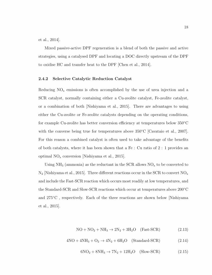
2.4.2 Selective Catalytic Reduction Catalyst

Reducing NOx emissions is often accomplished by the use of urea injection and a

SCR catalyst, normally containing either a Cu-zeolite catalyst, Fe-zeolite catalyst,

or a combination of both [Nishiyama et al., 2015]. There are advantages to using

either the Cu-zeolite or Fe-zeolite catalysts depending on the operating conditions,

for example Cu-zeolite has better conversion efficiency at temperatures below 350◦C

with the converse being true for temperatures above 350◦C [Cavataio et al., 2007].

For this reason a combined catalyst is often used to take advantage of the benefits

of both catalysts, where it has been shown that a Fe : Cu ratio of 2 : 1 provides an

optimal NOx conversion [Nishiyama et al., 2015].

Using NH3 (ammonia) as the reductant in the SCR allows NOx to be converted to

N2 [Nishiyama et al., 2015]. Three different reactions occur in the SCR to convert NOx

and include the Fast-SCR reaction which occurs most readily at low temperatures, and

the Standard-SCR and Slow-SCR reactions which occur at temperatures above 200◦C

and 275◦C , respectively. Each of the three reactions are shown below [Nishiyama

et al., 2015].

NO + NO2 + NH3 → 2N2 + 3H2O (Fast-SCR) (2.13)

4NO + 4NH3 + O2 → 4N2 + 6H2O (Standard-SCR) (2.14)

6NO2 + 8NH3 → 7N2 + 12H2O (Slow-SCR) (2.15)

19

Due to the toxicity of ammonia, NH3, and the difficulties associated with its

handling, Diesel exhaust fluid (DEF) or urea is instead added to the exhaust stream

which decomposes at high temperatures after being injected into the exhaust stream,

and forms NH3 by the reactions listed below [Nishiyama et al., 2015].

CO(NH2)2 → NH3 + HCNO (2.16)

HCNO + H2O→ NH3 + CO2 (2.17)

2.4.3 Diesel Oxidation Catalyst

The primary function of the DOC is to oxidize CO, HC and portions of the NO

emissions. As the oxidation of NO is equilibrium limited, the DOC oxidizes only por-

tions of the NO to alter the NO/NO2 ratio in the exhaust to meet the downstream

requirements of the SCR or LNT [Watling et al., 2012; Russell and Epling, 2011].

Precious metals are the most commonly used catalysts in the DOC, typically plat-

inum or palladium [Russell and Epling, 2011]. Each provide different advantages and

disadvantages depending on the operating conditions of the engine and the exhaust

composition and temperature.

The reactions occurring in the DOC are not fully understood as species interac-

tions and the competition for available O2 causes numerous intermediary reactions.

Watling et al. [2012] have developed a model of the reaction kinetics occurring inside

the DOC that illustrates the complicated species interactions that occur [Watling

et al., 2012].

The light-off temperature of a catalyst is normally defined by the inlet gas tem-

perature at which the catalyst can convert 50% of the intended reactant, known as

the T50 point (although other points may be cited) [Martin et al., 1998]. The light-off

20

temperature for the DOC is approximately 250◦C but depends on exhaust composi-

tion, the catalyst being used, and the construction of the DOC [Martin et al., 1998].

The importance of the light-off temperature is best exemplified by government legis-

lated test cycles, where it has been shown that 50% to 80% of emissions are produced

in the first 100 to 150 seconds prior to the catalyst reaching the light-off temperature

[Jeong and Kim, 1998; Shen et al., 1999; Cho et al., 1998]. Variables affecting the

light-off temperature of the DOC are the [Martin et al., 1998; Hayes et al., 2009]:

• composition of the catalyst

• age of the catalyst

• mass flow rate of exhaust gas

• exhaust gas temperature

• effective conductivity of the monolith

• flow maldistribution within the monolith

• bulk density of the monolith

• rate at which the inlet gas temperature increases

The complex interaction of all the variables involved in affecting the light-off

temperature of the catalyst make optimisation of the DOC difficult. Furthermore,

as the development of engines progresses, exhaust temperatures are becoming lower

leading to increased time before light-off is achieved [Bartley, 2015].

2.5 Catalyst Construction

This section details the construction and function of the DOC, providing a detailed

overview of the research that has focused on characterising the flow of exhaust through

the DOC.

21

2.5.1 Monolith Geometry

DOC design requirements vary from vehicle to vehicle depending on the manufactur-

ers requirements and optimization goals. The most common type of catalyst support

structure used in the automotive industry is the honeycomb monolith. The monolith

is composed of small channels in a honeycomb-like pattern running axially with the

flow of the exhaust, as shown in Figure 2.4. The shape of the channels can vary

depending on the requirements and benefits of each of the shapes. The cell geometry

affects the mass and strength of the substrate, the heat and mass transfer character-

istics, and flow resistance [Goralski and Chanko, 2001].

Figure 2.4: DOC showing the interior honeycomb like structure

Square, triangular, and hexagonal cells are the most common cell structures, how-

ever the final cell geometry is produced by the application of the washcoat to the

monolith. Numerous studies have shown that the washcoat is not applied uniformly

onto the substrate, rounding the corners of the cell and having a significant effect

on the performance of the monolith [Hayes et al., 2009; Goralski and Chanko, 2001].

Goralski and Chanko performed a series of tests to determine the optimal cell geom-

etry with washcoat applied and found that the hexagonal cells tend to have a higher

conversion efficiency while each of the channel geometries showed a similar maximum

effective loading [Goralski and Chanko, 2001]. Furthermore, they showed that hexag-

onal and square channels would show a similar pressure drop for exhaust flow rates

typical of those seen in automobiles [Goralski and Chanko, 2001].

22

2.5.2 Flow Distribution

The flow through the DOC is complex and finding an optimal overall geometry diffi-

cult. The DOC can be broken into five sections and are shown in Figure 2.5; the inlet

pipe (1), the inlet cone (2), the body (3), the outlet cone (4), and the outlet pipe (5).

12

3

54

Flow Direction

Figure 2.5: Schematic of the components that make up the DOC (axisymmetric)

The inlet and outlet pipes are the exhaust pipes that connect the DOC to the

engine and the tailpipe, respectively. The inlet cone is an expansion cone (axisym-

metric conical diffuser) that increases the diameter from that of the inlet pipe to that

of the monolith. The body is composed of the honeycomb structure containing the

catalyst, known as the monolith. The outlet cone is a compression cone (axisymmet-

ric contraction) that decreases the diameter from the diameter of the body back to

the diameter of the exhaust pipe.

2.5.3 Inlet/Outlet Flow

As the flow enters the inlet diffusers upstream of the monolith, the flow becomes even

more turbulent and non-uniform as it expands with the increasing pipe diameter,

resulting in a flow maldistribution over the radial profile of the DOC [Litto et al.,

2016; Cho et al., 1998]. The flow through a diffuser is affected by three parameters: the

half angle of the diffuser, the diffuser length to width ratio, and the turbulence of the

flow into the diffuser, while the Reynolds number of the inlet flow was found to have

23

no effect for turbulent flow [Fox and Kline, 1962]. Fox and Kline [1962] demonstrated

the relationlship between the diffuser half angle and the length to width ratios [Fox

and Kline, 1962].

Fox and Kline [1962] were able to demonstrate that with increasing diffuser angle

there exists a threshold where stall occurs. The greater the increase in half angle

above the transition results in more fluid undergoing stall leading to larger degrees

of turbulence. The stalled fluid along the walls creates a blockage that forces the

flow to detour around the blockage and at sufficiently large amounts of stall a jet is

created through the centre of the diffuser [Kline and Johnston, 1986]. The resulting

flow maldistribution leads to the following negative effects [Cho et al., 1998; Jeong

and Kim, 1998; Martin et al., 1998]:

• poor catalyst conversion efficiency

• premature ageing of the catalyst

• increased time to reach catalyst light-off

• increased pressure drop across the DOC

The flow maldistribution is often characterized by the flow uniformity index, γ,

given by,

γ = 1− 1

2n

n∑i=1

√(ui − u)2

u(2.18)

where ui is the local flow velocity of the ith area, u is the average velocity, and n is

the total number of areas being considered [Cho et al., 1998]. Flow uniformity index

values range from 0.7 to 0.98 for most catalytic converters, with values under 0.8

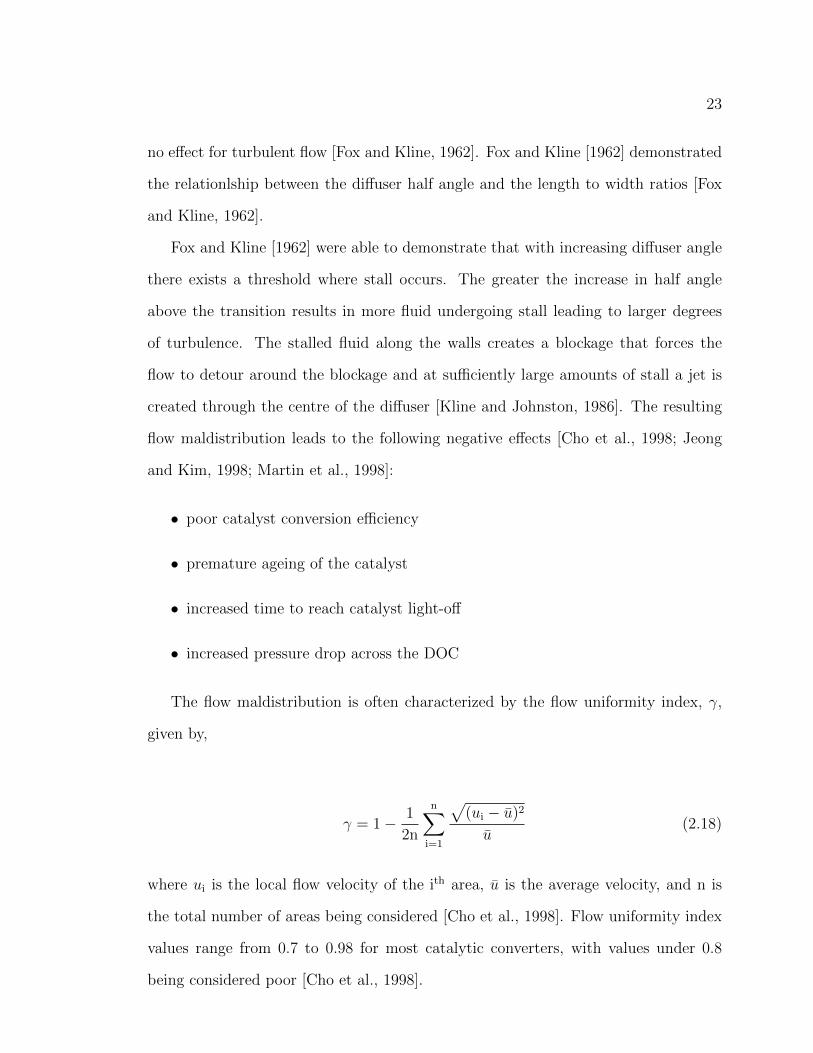
being considered poor [Cho et al., 1998].

24

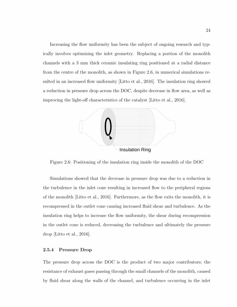
Increasing the flow uniformity has been the subject of ongoing research and typ-

ically involves optimizing the inlet geometry. Replacing a portion of the monolith

channels with a 3 mm thick ceramic insulating ring positioned at a radial distance

from the centre of the monolith, as shown in Figure 2.6, in numerical simulations re-

sulted in an increased flow uniformity [Litto et al., 2016]. The insulation ring showed

a reduction in pressure drop across the DOC, despite decrease in flow area, as well as

improving the light-off characteristics of the catalyst [Litto et al., 2016].

Figure 2.6: Positioning of the insulation ring inside the monolith of the DOC

Simulations showed that the decrease in pressure drop was due to a reduction in

the turbulence in the inlet cone resulting in increased flow to the peripheral regions

of the monolith [Litto et al., 2016]. Furthermore, as the flow exits the monolith, it is

recompressed in the outlet cone causing increased fluid shear and turbulence. As the

insulation ring helps to increase the flow uniformity, the shear during recompression

in the outlet cone is reduced, decreasing the turbulence and ultimately the pressure

drop [Litto et al., 2016].

2.5.4 Pressure Drop

The pressure drop across the DOC is the product of two major contributors; the

resistance of exhaust gases passing through the small channels of the monolith, caused

by fluid shear along the walls of the channel, and turbulence occurring in the inlet

25

and outlet cones, due to the sudden expansion and contraction of the exhaust gases.

The pressure drop due to shear along the walls of the monolith is proportional to the

fluid velocity, increasing as the velocity increases [Karvounis and Assanis, 1993].

It is common for numerical simulations to approximate the flow through the mono-

lith as being fully-developed laminar flow over its entire length and to ignore turbu-

lence. Turbulence in the monolith is primarily the result of three sources; turbulence

originating upstream of the monolith in the diffuser, turbulence created by the channel

walls at the entrance to the monolith, and turbulence caused by the surface roughness

along the length of the channel walls [Holmgren and Andersson, 1998].

When laminar flow through the monolith channel is assumed, the flow through

the monolith is Hagen-Poiseuille flow and the pressure drop in the channels of the

monolith is the result of viscous forces [Ozhan et al., 2014] and the pressure drop,

∆P , can be approximated by Poiseuille’s law,

∆P =8µLcQc

πDc4 (2.19)

where Lc and Dc is the monolith channel length and hydraulic diameter, respectively,

µ is the fluid viscosity, and Qc is the average volumetric flow rate in a single channel

[Ozhan et al., 2014].

However, the pressure drop across the DOC is affected by turbulence in the inlet

diffuser and outlet nozzle. Turbulence models commonly used to simulate flow across

the DOC include the k-ε model [Karvounis and Assanis, 1993; Holmgren et al., 1997;

Hayes et al., 2012] and the k-ω model [Litto et al., 2016].

To reduce the computational requirements of modeling the flow through each of the

monolith channels, the monolith is modeled as a porous region consisting of strictly

laminar flow [Karvounis and Assanis, 1993]. The assumption of laminar flow in the

26

monolith is not entirely valid as turbulence has been found to persist beyond the

entrance of the monolith, however the effect on the pressure drop across the monolith

has been shown to be very small [Cornejo et al., 2017]. The Forcheimer’s modified

formulation of Darcy’s equation is included as a source term, ~S, in the conservation

of momentum equation and is given by,

~S =

(µ

α+ρC2|~v|

2

)~v (2.20)

where µ is the dynamic viscosity, 1/α and C2 are the viscous and inertial resistance

factors. With the flow through the monolith being assumed laminar, the inertial

resistance factor is set to zero as turbulence is not present. The viscous factor can be

found either theoretically or empirically by either calculating the pressure drop using

Equation 2.19 or by using experimental pressure drop data. Knowing the pressure

drop, the viscous resistance factor can be related to the source term by simplifying

the momentum equation to yield [ANSYS, Inc., 2006]

∆P = −S · L = −µα~v · L (2.21)

where L is the length of the channel.

To simulate the unidirectional flow through the monolith, the viscous resistance

terms in the radial direction are set to a minimum of three orders of magnitude larger

than the axial direction [Karvounis and Assanis, 1993].

27

2.5.5 Monolith Temperature

The radial temperature profile of the monolith is affected by the exhaust gas temper-

ature, the effective conductivity of the monolith, the exhaust composition, and the

flow uniformity. Reactions occurring along the surface of the monolith channels which

contain the catalyst are limited by two factors; the rate of reaction and the rate of

mass transfer [Karvounis and Assanis, 1993]. While the monolith is initially at ambi-

ent temperature, the conversion rate of the catalyst is limited by the rate of reaction.

Once the exhaust gases have sufficiently heated the monolith, the rate limiting factor

in the conversion rate switches from rate of reaction to rate of mass transfer. Due to

the difficulty in determining the exact temperature in which this switch occurs, the

light-off temperature is often used as an approximation of this switch.

A number of factors can affect the ability for the catalyst to reach light-off, includ-

ing the exhaust temperature and the flow uniformity. The exhaust gas temperature

has a large affect on the time required for the catalyst to reach light-off and as auto-

motive exhaust temperatures become lower, there is evidence that vehicles are unable

to meet emissions standards due to their inabiliy to reach light-off in a reasonable

time [Bartley, 2015]. The exhaust composition can also play a role in the time re-

quired to reach light-off, as certain molecules inhibit the ability of reactants to react

on the catalyst, leading to a decrease in conversion efficiency and an increase in the

light-off temperature [Bartley, 2015].

The radial temperature profile of the monolith is affected by the effective con-

ductivity of the monolith and the flow uniformity. The effective conductivity of the

monolith can be approximated using the electrical resistances analogy [Hayes et al.,

2009]. When the monolith construction is changed, for example by adding an insu-

lation ring, as discussed in Section 2.5.3, the effective conductivity causes a change

in the radial temperature profile [Hayes et al., 2009]. The insulation ring results in a

28

decrease in time required to reach light-off as the insulation ring maintains the heat

in the central region of the monolith and at low load (as is typical during vehicle

warm-up) the majority of the exhaust gases are directed through the central region

of the monolith [Litto et al., 2016] due to the effect of a jet being created in the inlet

diffuser (see Section 2.5.2. As the central region of the monolith heats up faster and

the majority of the flow passes through the central region, emissions can be reduced.

29

Chapter 3

Experimental Setup

This Chapter details the experimental setup used and includes a detailed explanation

of the Diesel engine along with modifications, the engine dynamometer, the exhaust

setup, the geometry and assembly of the DOC, and the sensors used for data collection.

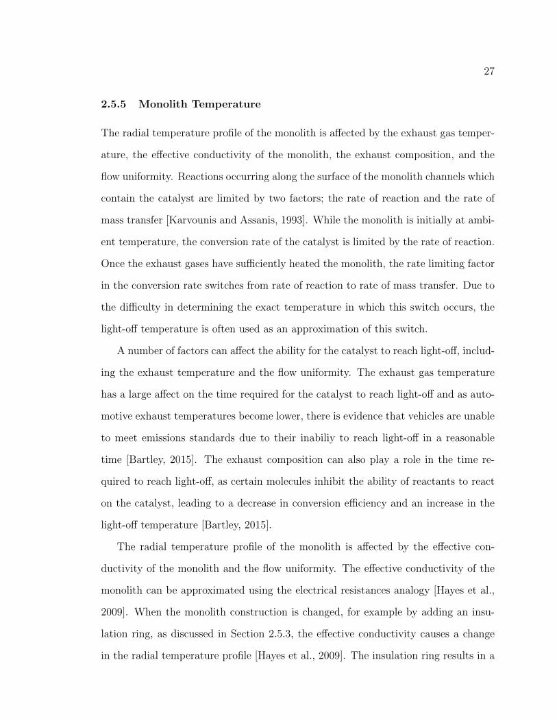
3.1 Experimental Setup

The primary objective of the experiment was to characterize the flow of exhaust

gas as it passed through the DOC and to determine the heating characteristics of

the DOC. The DOC is connected to a stock Cummins 4-cylinder Diesel engine (see

Section 3.2) and a Tornado centrifugal fan with 6.5 HP electric motor, giving the

option of directing hot exhaust gas from the engine or cold air from the blower

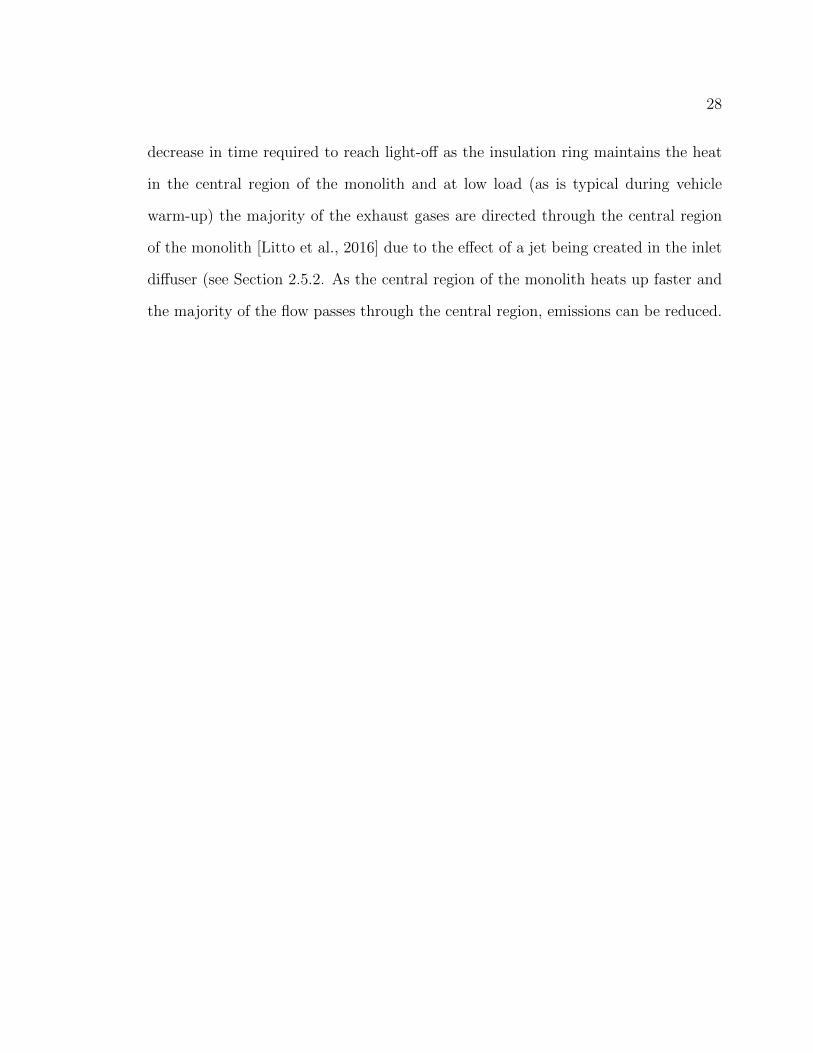
through the DOC. By opening or closing the correct configuration of valves, as shown

in Figures 3.1 and 3.2, the gas passing through the DOC can be easily switched

between hot from the engine or cold from the blower.

The hot exhaust gas can be bypassed around the DOC allowing the engine to reach

steady state operation with a constant exhaust temperature prior to directing the gas

through the DOC. After passing through the DOC, the exhaust gasses pass through

a muffler and then are exhausted into an open exhaust conduit drawing exhaust in

at slightly lower pressure than the ambient room pressure, as shown in Figure 3.2.

30

Engine

BlowerBypass

DOC

Pitot Tube

Valve

Figure 3.1: Exhaust bypass setup

Figure 3.2: Schematic of the experimental setup

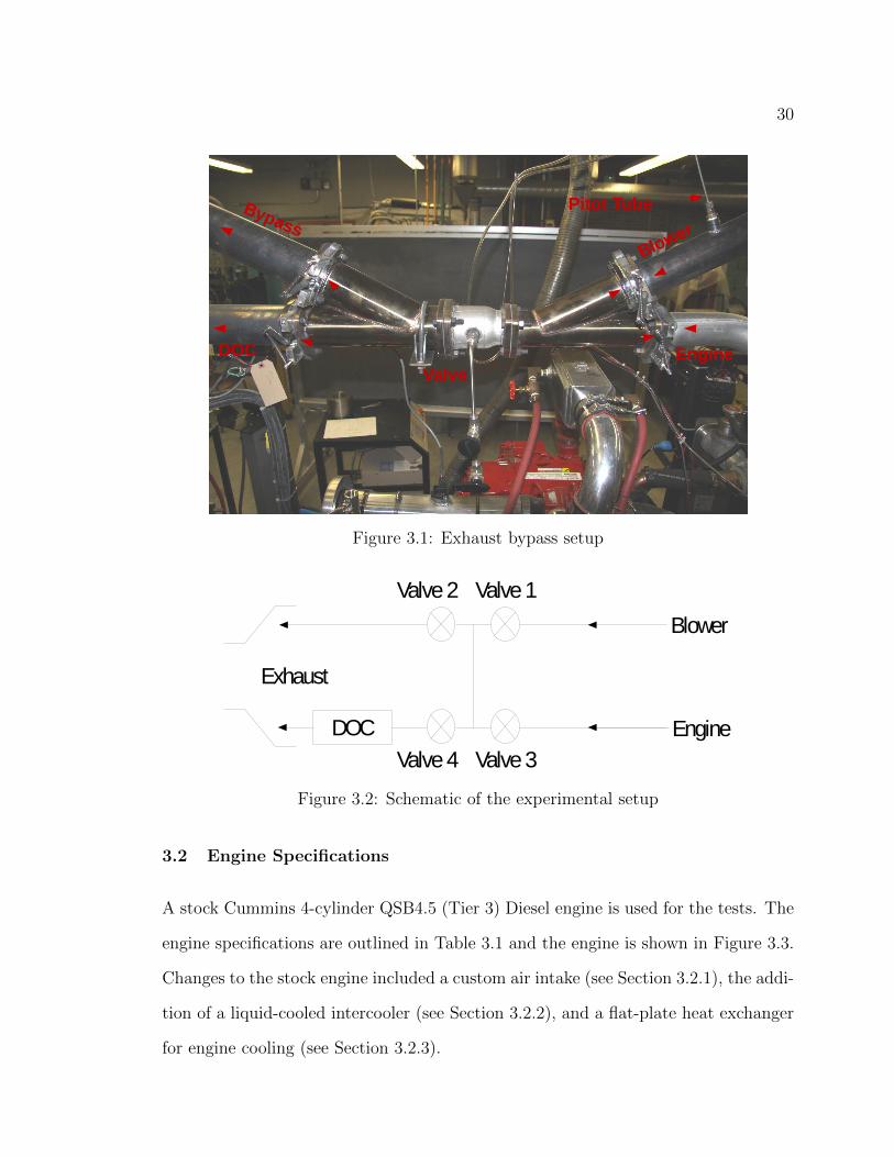
3.2 Engine Specifications

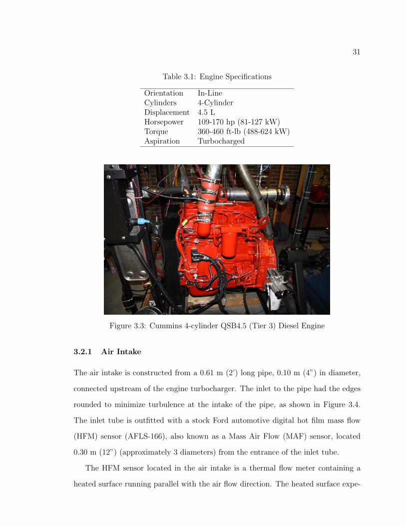
A stock Cummins 4-cylinder QSB4.5 (Tier 3) Diesel engine is used for the tests. The

engine specifications are outlined in Table 3.1 and the engine is shown in Figure 3.3.

Changes to the stock engine included a custom air intake (see Section 3.2.1), the addi-

tion of a liquid-cooled intercooler (see Section 3.2.2), and a flat-plate heat exchanger

for engine cooling (see Section 3.2.3).

31

Table 3.1: Engine Specifications

Orientation In-LineCylinders 4-CylinderDisplacement 4.5 LHorsepower 109-170 hp (81-127 kW)Torque 360-460 ft-lb (488-624 kW)Aspiration Turbocharged

Figure 3.3: Cummins 4-cylinder QSB4.5 (Tier 3) Diesel Engine

3.2.1 Air Intake

The air intake is constructed from a 0.61 m (2’) long pipe, 0.10 m (4”) in diameter,

connected upstream of the engine turbocharger. The inlet to the pipe had the edges

rounded to minimize turbulence at the intake of the pipe, as shown in Figure 3.4.

The inlet tube is outfitted with a stock Ford automotive digital hot film mass flow

(HFM) sensor (AFLS-166), also known as a Mass Air Flow (MAF) sensor, located

0.30 m (12”) (approximately 3 diameters) from the entrance of the inlet tube.

The HFM sensor located in the air intake is a thermal flow meter containing a

heated surface running parallel with the air flow direction. The heated surface expe-

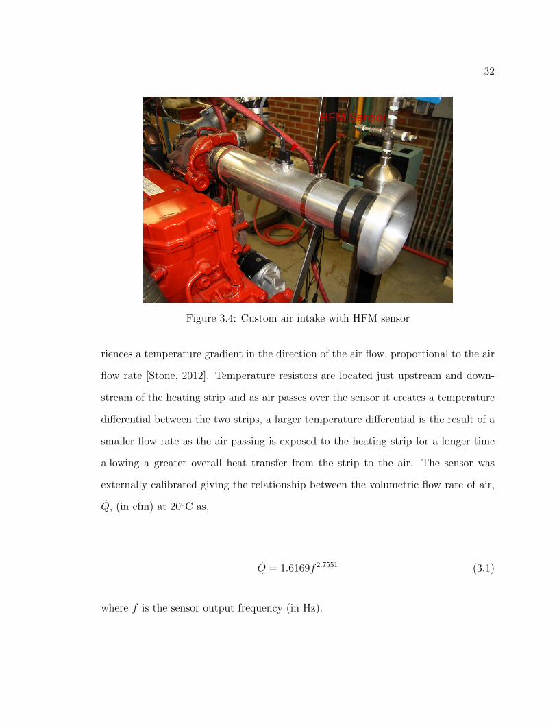
32

HFM Sensor

Figure 3.4: Custom air intake with HFM sensor

riences a temperature gradient in the direction of the air flow, proportional to the air

flow rate [Stone, 2012]. Temperature resistors are located just upstream and down-

stream of the heating strip and as air passes over the sensor it creates a temperature

differential between the two strips, a larger temperature differential is the result of a

smaller flow rate as the air passing is exposed to the heating strip for a longer time

allowing a greater overall heat transfer from the strip to the air. The sensor was

externally calibrated giving the relationship between the volumetric flow rate of air,

Q, (in cfm) at 20◦C as,

Q = 1.6169f 2.7551 (3.1)

where f is the sensor output frequency (in Hz).

33

3.2.2 Air Intake Temperature Control

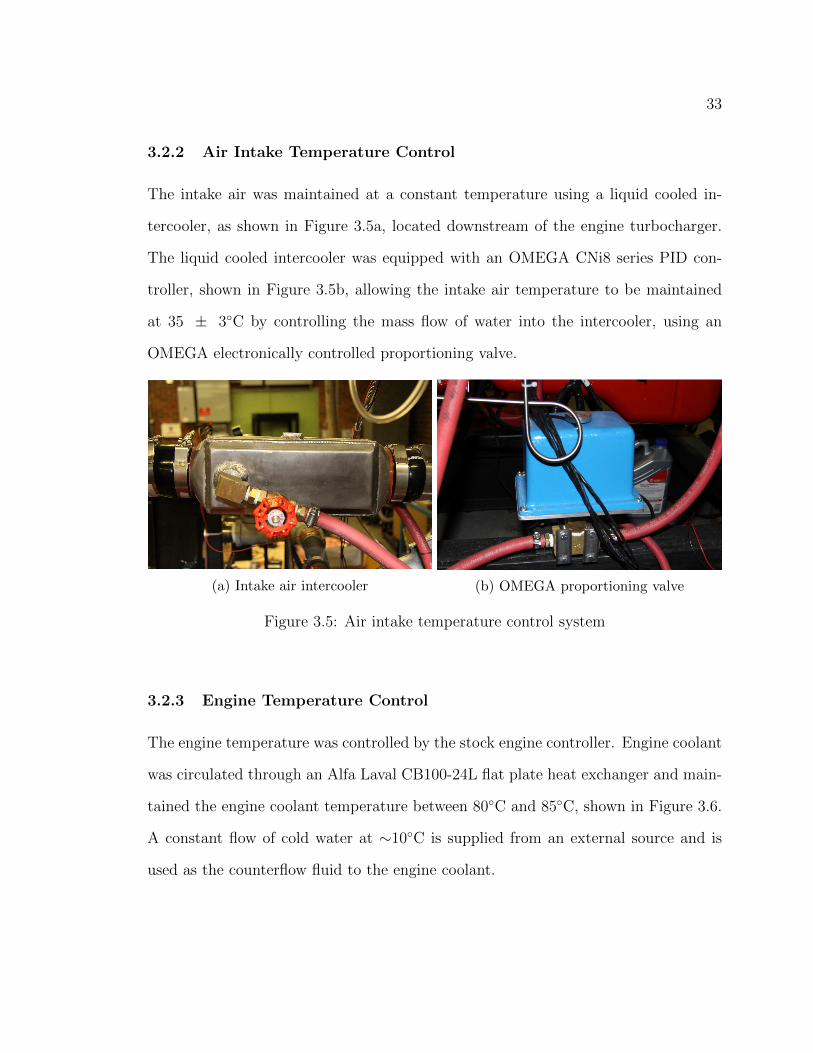
The intake air was maintained at a constant temperature using a liquid cooled in-

tercooler, as shown in Figure 3.5a, located downstream of the engine turbocharger.

The liquid cooled intercooler was equipped with an OMEGA CNi8 series PID con-

troller, shown in Figure 3.5b, allowing the intake air temperature to be maintained

at 35 ± 3◦C by controlling the mass flow of water into the intercooler, using an

OMEGA electronically controlled proportioning valve.

(a) Intake air intercooler (b) OMEGA proportioning valve

Figure 3.5: Air intake temperature control system

3.2.3 Engine Temperature Control

The engine temperature was controlled by the stock engine controller. Engine coolant

was circulated through an Alfa Laval CB100-24L flat plate heat exchanger and main-

tained the engine coolant temperature between 80◦C and 85◦C, shown in Figure 3.6.

A constant flow of cold water at ∼10◦C is supplied from an external source and is

used as the counterflow fluid to the engine coolant.

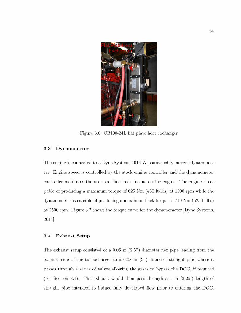
34

Flat PlateHeatExchanger

Figure 3.6: CB100-24L flat plate heat exchanger

3.3 Dynamometer

The engine is connected to a Dyne Systems 1014 W passive eddy current dynamome-

ter. Engine speed is controlled by the stock engine controller and the dynamometer

controller maintains the user specified back torque on the engine. The engine is ca-

pable of producing a maximum torque of 625 Nm (460 ft-lbs) at 1900 rpm while the

dynamometer is capable of producing a maximum back torque of 710 Nm (525 ft-lbs)

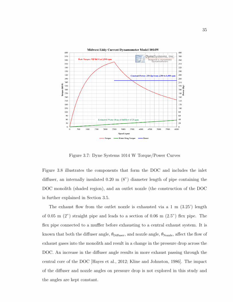
at 2500 rpm. Figure 3.7 shows the torque curve for the dynamometer [Dyne Systems,

2014].

3.4 Exhaust Setup

The exhaust setup consisted of a 0.06 m (2.5”) diameter flex pipe leading from the

exhaust side of the turbocharger to a 0.08 m (3”) diameter straight pipe where it

passes through a series of valves allowing the gases to bypass the DOC, if required

(see Section 3.1). The exhaust would then pass through a 1 m (3.25’) length of

straight pipe intended to induce fully developed flow prior to entering the DOC.

35

Figure 3.7: Dyne Systems 1014 W Torque/Power Curves

Figure 3.8 illustrates the components that form the DOC and includes the inlet

diffuser, an internally insulated 0.20 m (8”) diameter length of pipe containing the

DOC monolith (shaded region), and an outlet nozzle (the construction of the DOC

is further explained in Section 3.5.

The exhaust flow from the outlet nozzle is exhausted via a 1 m (3.25’) length

of 0.05 m (2”) straight pipe and leads to a section of 0.06 m (2.5”) flex pipe. The

flex pipe connected to a muffler before exhausting to a central exhaust system. It is

known that both the diffuser angle, θDiffuser, and nozzle angle, θNozzle, affect the flow of

exhaust gases into the monolith and result in a change in the pressure drop across the

DOC. An increase in the diffuser angle results in more exhaust passing through the

central core of the DOC [Hayes et al., 2012; Kline and Johnston, 1986]. The impact

of the diffuser and nozzle angles on pressure drop is not explored in this study and

the angles are kept constant.

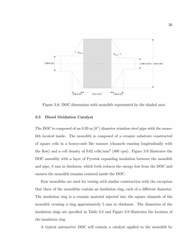
36

0.06 m (2.5”)0.08 m (3”) 0.20 m (8”)

θDiffuser

θNozzle

0.08 m (3”) 0.08 m (3”)0.01 m (4”)

Figure 3.8: DOC dimensions with monolith represented by the shaded area

3.5 Diesel Oxidation Catalyst

The DOC is composed of an 0.20 m (8”) diameter stainless steel pipe with the mono-

lith located inside. The monolith is composed of a ceramic substrate constructed

of square cells in a honeycomb like manner (channels running longitudinally with

the flow) and a cell density of 0.62 cells/mm2 (400 cpsi). Figure 3.9 illustrates the

DOC assembly with a layer of Pyrotek expanding insulation between the monolith

and pipe, 8 mm in thickness, which both reduces the energy lost from the DOC and

ensures the monolith remains centered inside the DOC.

Four monoliths are used for testing with similar construction with the exception

that three of the monoliths contain an insulation ring, each of a different diameter.

The insulation ring is a ceramic material injected into the square channels of the

monolith creating a ring approximately 5 mm in thickness. The diameters of the

insulation rings are specified in Table 3.2 and Figure 3.9 illustrates the location of

the insulation ring.

A typical automotive DOC will contain a catalyst applied to the monolith by

37

PyrotekInsulation

Honeycomb Monolith

InsulationRing

SS Pipe

Figure 3.9: Structure of the DOC (shown in cross section)

Table 3.2: Inside and outside diameters of monolith insulation rings

DOC Description ID (mm) OD (mm)1 No Insulation Ring N/A N/A2 Small Insulation Ring 41 ± 2 46 ± 23 Medium Insulation Ring 70 ± 2 75 ± 24 Large Insulation Ring 99 ± 2 104 ± 2

submersing the monolith in a liquid containing the catalyst, known as the washcoat,

which is then cured onto the monolith. None of the four monolith have had a washcoat

applied as the flow characteristics through the monolith are the parameters of interest

and not the reaction kinetics, therefore no active catalyst is present. The DOC

construction (without diffuser/nozzle) is shown in Figure 3.9.

3.6 Sensors

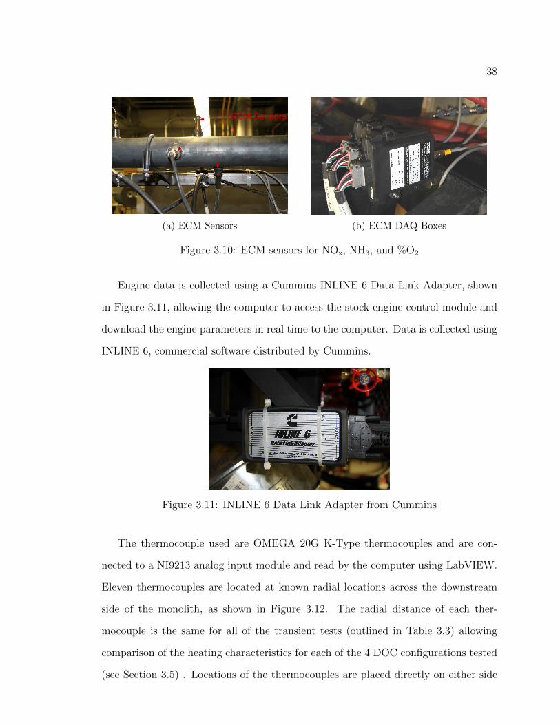
Exhaust composition is determined using NOxCANt ECM sensors, shown in Fig-

ure 3.10a, and includes a NOx sensor, NH3 sensor, and O2 sensor. The sensors are

located 0.30 m, 0.35 m, and 0.40 m upstream of the entrance to the diffuser, respec-

tively. The ECM sensors are connected via an ECM CAN line, shown in Figure 3.10b,

to the computer for data collection using Kvaser Leaf Light HS.

38

ECM Sensors

(a) ECM Sensors (b) ECM DAQ Boxes

Figure 3.10: ECM sensors for NOx, NH3, and %O2

Engine data is collected using a Cummins INLINE 6 Data Link Adapter, shown

in Figure 3.11, allowing the computer to access the stock engine control module and

download the engine parameters in real time to the computer. Data is collected using

INLINE 6, commercial software distributed by Cummins.

Figure 3.11: INLINE 6 Data Link Adapter from Cummins

The thermocouple used are OMEGA 20G K-Type thermocouples and are con-

nected to a NI9213 analog input module and read by the computer using LabVIEW.

Eleven thermocouples are located at known radial locations across the downstream

side of the monolith, as shown in Figure 3.12. The radial distance of each ther-

mocouple is the same for all of the transient tests (outlined in Table 3.3) allowing

comparison of the heating characteristics for each of the 4 DOC configurations tested

(see Section 3.5) . Locations of the thermocouples are placed directly on either side

39

of the insulation as well as midway between the insulation rings (if they were to all be

superimposed onto the same monolith). There are also three thermocouples located

in the exhaust piping; one thermocouple is located immediately downstream of the

exhaust manifold, one 0.15 m upstream of the entrance to the diffuser, and one 0.15 m

downstream of the exit to the diffuser, as shown in Figure 3.13.

r = 0

Figure 3.12: Locations of thermocouples in the monolith (shown in cross section)

Table 3.3: Radial location of thermocouples in monolith

Radial LocationThermocouple (mm)

1 02 183 224 285 346 407 438 479 5310 7111 90

40

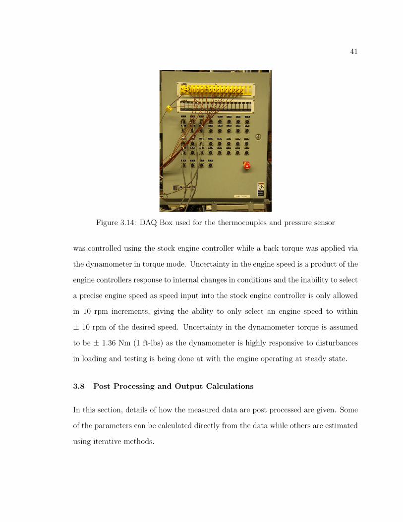
The differential pressure sensor is a stock automotive pressure sensor with a linear

relationship between the voltage output and a change in pressure. The pressure taps

are located 0.15 m upstream and downstream of the DOC, as shown in Figure 3.13.

The pressure sensor is calibrated to give the following relationship between the output

voltage, V out, (in Volts) and the differential pressure, ∆P, (in kPa),

∆P = 2.7185V out − 6.9283 (3.2)

The output voltage from the pressure sensor is collected via a NI9205 analog input

module and collected by a computer using the commercial software LabVIEW. The

sampling rate for all of the variables was set to 1 Hz as the time constant of the DOC

temperature is much longer than 1 Hz allowing the dynamic response of the DOC to

be easily captured.

Figure 3.13: Exhaust setup showing the sensors and data acquisition equipment

3.7 Operating Points

Engine operating points were selected to span the engines operating range by varying

both the speed and load. The operating points are outlined in Table 3.4. Engine speed

41

Figure 3.14: DAQ Box used for the thermocouples and pressure sensor

was controlled using the stock engine controller while a back torque was applied via

the dynamometer in torque mode. Uncertainty in the engine speed is a product of the

engine controllers response to internal changes in conditions and the inability to select

a precise engine speed as speed input into the stock engine controller is only allowed

in 10 rpm increments, giving the ability to only select an engine speed to within

± 10 rpm of the desired speed. Uncertainty in the dynamometer torque is assumed

to be ± 1.36 Nm (1 ft-lbs) as the dynamometer is highly responsive to disturbances

in loading and testing is being done at with the engine operating at steady state.

3.8 Post Processing and Output Calculations

In this section, details of how the measured data are post processed are given. Some

of the parameters can be calculated directly from the data while others are estimated

using iterative methods.

42

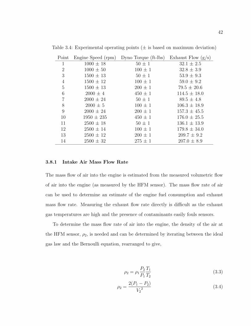
Table 3.4: Experimental operating points (± is based on maximum deviation)

Point Engine Speed (rpm) Dyno Torque (ft-lbs) Exhaust Flow (g/s)1 1000 ± 18 50 ± 1 32.1 ± 2.52 1000 ± 50 100 ± 1 32.8 ± 3.93 1500 ± 13 50 ± 1 53.9 ± 9.34 1500 ± 12 100 ± 1 59.0 ± 9.25 1500 ± 13 200 ± 1 79.5 ± 20.66 2000 ± 4 450 ± 1 114.5 ± 18.07 2000 ± 24 50 ± 1 89.5 ± 4.88 2000 ± 5 100 ± 1 106.3 ± 18.99 2000 ± 24 200 ± 1 157.3 ± 45.510 1950 ± 235 450 ± 1 176.0 ± 25.511 2500 ± 18 50 ± 1 136.1 ± 13.912 2500 ± 14 100 ± 1 179.8 ± 34.013 2500 ± 12 200 ± 1 209.7 ± 9.214 2500 ± 32 275 ± 1 207.0 ± 8.9

3.8.1 Intake Air Mass Flow Rate

The mass flow of air into the engine is estimated from the measured volumetric flow

of air into the engine (as measured by the HFM sensor). The mass flow rate of air

can be used to determine an estimate of the engine fuel consumption and exhaust

mass flow rate. Measuring the exhaust flow rate directly is difficult as the exhaust

gas temperatures are high and the presence of contaminants easily fouls sensors.

To determine the mass flow rate of air into the engine, the density of the air at

the HFM sensor, ρ2, is needed and can be determined by iterating between the ideal

gas law and the Bernoulli equation, rearranged to give,

ρ2 = ρ1P2

P1

T1

T2

(3.3)

ρ2 =2(P1 − P2)

V22 (3.4)

43

where P1, T1, and ρ1 are the atmospheric air pressure, temperature, and den-

sity,respectively, and P2, T2, and ρ2 are the air pressure, temperature, and density,

respectively, at the HFM sensor inside the air intake. The velocity of air at the HFM

sensor, V2, is calculated using the volumetric flow rate and cross-sectional area. The

form of the Bernoulli equation assumes incompressible flow and as the velocity of the

air at the HFM sensor is less than 1/10th the speed of sound, the error introduced

is known to be small [Yunus and Cimbala, 2006]. The atmospheric pressure, P1, and

temperature, T1 are measured at the beginning of each test and the temperature in

the intake was assumed to be the same as the atmospheric temperature, as expan-

sion effects are assumed to be minimal. The velocity of air into the intake, V1, is

approximated to be zero (large reservoir assumption).

3.8.2 Exhaust Mass Flow Rate

The mass flow rate of exhaust was estimated using the sum of the intake air mass

flow rate and the mass flow rate of fuel into the engine. The flow rate of exhaust is

difficult to measure directly as the conditions in the exhaust are not conducive to mass

flow sensors since the exhaust contains large amounts of particulate, which rapidly

foul the sensor, and the high temperature which affect the material properties of the

sensor. The mass flow rate of fuel into the engine can be be estimated by using the

intake air mass flow rate and finding the difference in oxygen concentration between

the exhaust and atmosphere.

The exhaust oxygen concentration is measured by the ECM sensors, located in the

exhaust pipe just upstream of the DOC, while the atmospheric oxygen concentration

is assumed to be 20%. Furthermore, combustion is assumed to be stoichiometric and

the fuel is assumed to be composed solely C12H23. The mass flow rate of the exhaust

is then estimated by,

44

mexhaust = mair,in

[1 +

(YO2,in

− YO2,exhaust

)(17.75

molO2

molC12H23

)MO2

MC12H23

](3.5)

where YO2,in is the molar atmospheric oxygen concentration, YO2,exhaust is the molar

exhaust oxygen concentration, 17.75 molO2/molC12H23 is the molar ratio of oxygen to

fuel in stoichiometric combustion of C12H23.

Many assumptions were made in determining the mass flow rate of exhaust and

to validate the results of the calculation, an engine test was performed measuring the

intake air flow rate via the HFM sensor while the mass flow rate of fuel was measured

by placing the fuel tank on a scale and measuring its weight over time. Figure 3.15

illustrates the mass flow rates of fuel and air, showing that the mass flow rate of air

into the engine is one to two orders of magnitude larger, depending on the operating

point, suggesting that error introduced into the calculation of the mass flow rate of

fuel is small compared to the overall mass flow rate of exhaust. Furthermore, as the

fuel consumption is nearly identical between each of the four DOC configurations

for a given operating point, the error introduced will be similar allowing comparison

between the DOC configurations.

3.9 Engine Facility Setup

This section details additions to the engine facility that will be used for future exper-

imental testing.

3.9.1 Ammonia Injection

An ammonia injection system was added to the Diesel exhaust setup for future SCR

catalyst testing and ammonia sensor testing. The setup consist of a reservoir contain-

ing 30% aqueous ammonia (although any concentration could be used). Compressed

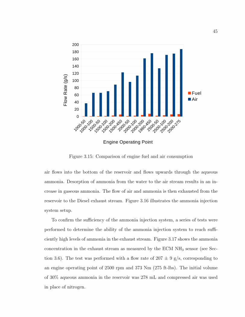
45

Figure 3.15: Comparison of engine fuel and air consumption

air flows into the bottom of the reservoir and flows upwards through the aqueous

ammonia. Desorption of ammonia from the water to the air stream results in an in-

crease in gaseous ammonia. The flow of air and ammonia is then exhausted from the

reservoir to the Diesel exhaust stream. Figure 3.16 illustrates the ammonia injection

system setup.

To confirm the sufficiency of the ammonia injection system, a series of tests were

performed to determine the ability of the ammonia injection system to reach suffi-

ciently high levels of ammonia in the exhaust stream. Figure 3.17 shows the ammonia

concentration in the exhaust stream as measured by the ECM NH3 sensor (see Sec-

tion 3.6). The test was performed with a flow rate of 207 ± 9 g/s, corresponding to

an engine operating point of 2500 rpm and 373 Nm (275 ft-lbs). The initial volume

of 30% aqueous ammonia in the reservoir was 278 mL and compressed air was used

in place of nitrogen.

46

Figure 3.16: Schematic of the ammonia injection system

Figure 3.17: Ammonia concentration in the exhaust stream

Figure 3.17 illustrates that the ammonia injection system is easily capable of

delivering the required 300 ppm of ammonia to the exhaust stream. With the addition

of a controller, using the ammonia concentration in the exhaust as the reference and

the nitrogen regulator regulating the flow into the reservoir, as the actuator.

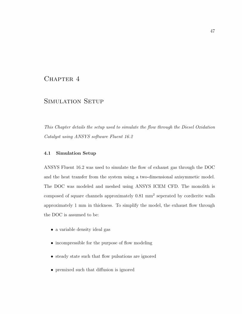
47

Chapter 4

Simulation Setup

This Chapter details the setup used to simulate the flow through the Diesel Oxidation

Catalyst using ANSYS software Fluent 16.2

4.1 Simulation Setup

ANSYS Fluent 16.2 was used to simulate the flow of exhaust gas through the DOC

and the heat transfer from the system using a two-dimensional axisymmetic model.

The DOC was modeled and meshed using ANSYS ICEM CFD. The monolith is

composed of square channels approximately 0.81 mm2 seperated by cordierite walls

approximately 1 mm in thickness. To simplify the model, the exhaust flow through

the DOC is assumed to be:

• a variable density ideal gas

• incompressible for the purpose of flow modeling

• steady state such that flow pulsations are ignored

• premixed such that diffusion is ignored

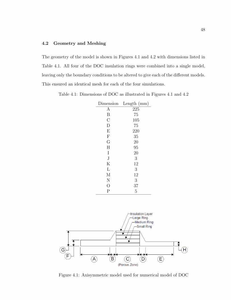
48

4.2 Geometry and Meshing

The geometry of the model is shown in Figures 4.1 and 4.2 with dimensions listed in

Table 4.1. All four of the DOC insulation rings were combined into a single model,

leaving only the boundary conditions to be altered to give each of the different models.

This ensured an identical mesh for each of the four simulations.

Table 4.1: Dimensions of DOC as illustrated in Figures 4.1 and 4.2

Dimension Length (mm)A 225B 75C 105D 75E 220F 35G 20H 95I 20J 3K 12L 3M 12N 3O 37P 5

Figure 4.1: Axisymmetric model used for numerical model of DOC

49

Figure 4.2: Detailed geometry of porous zone (see Figure 4.1)

The geometry is broken into a series of blocks for meshing. Along the horizontal

axis the mesh is broken into five blocks, corresponding to each of the regions labelled

A through E in Figure 4.1. Along the vertical axis the mesh is broken into eight

blocks corresponding to each of the regions labelled I through P in Figure 4.2. The

mesh is sized to obtain a maximum mesh sizing of 0.5 mm within the monolith of the

DOC (region C) while the mesh inside the inlet and outlet pipe (regions A and E) is

sized proportionally to the monolith and ensures that the elements remain the same

size regardless of the vertical location, resulting in elements that are evenly spaced

along both the vertical and horizontal axes. The mesh sizes are outlined in Table 4.2.

4.2.1 Material Properties

The material properties for each of the components of the DOC are listed in Table 4.3.

As the material properties are not known accurately, they were adjusted slightly to

improve the fit between the numerical analysis and experimental results. The shell

of the DOC is constructed from 1/32” stainless steel (SS310), the insulation between

the shell and monolith is 3/16” Pyrotek R© IR-3, the monolith is cordierite, and the

insulation ring is created by injecting ceramic into the channels of the monolith.

50

Figure 4.3: DOC meshing using ANSYS ICEM to create structured mesh

Table 4.2: Mesh sizing by component

Dimension Nodes Max Mesh Size (mm) Min Mesh SizeA 751 0.30 0.30B 164 0.49 0.30C 211 0.51 0.51D 164 0.48 0.29E 734 0.30 0.30I 41 0.50 0.19J 7 0.50 0.19K 25 0.50 0.18L 7 0.50 0.18M 25 0.50 0.18N 7 0.50 0.18O 75 0.50 0.19P 11 0.50 0.18

4.3 Heat Transfer

The heat transfer from the DOC to the surroundings was modeled using a natural

convection model. The wall was constructed of stainless steel (SS310), an overall heat

transfer coefficient of 15 W/(m-K) was used along with a free stream temperature of

305 K. Radiation from the DOC was ignored as it was assumed to be small.

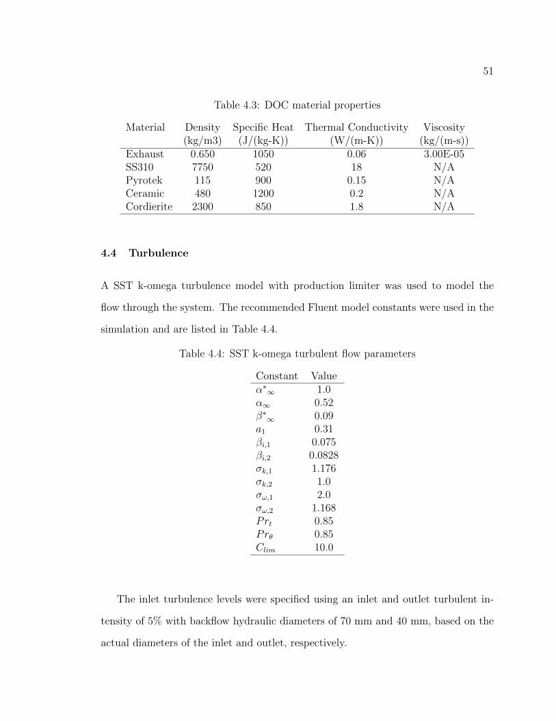
51

Table 4.3: DOC material properties

Material Density Specific Heat Thermal Conductivity Viscosity(kg/m3) (J/(kg-K)) (W/(m-K)) (kg/(m-s))

Exhaust 0.650 1050 0.06 3.00E-05SS310 7750 520 18 N/APyrotek 115 900 0.15 N/ACeramic 480 1200 0.2 N/ACordierite 2300 850 1.8 N/A

4.4 Turbulence

A SST k-omega turbulence model with production limiter was used to model the

flow through the system. The recommended Fluent model constants were used in the

simulation and are listed in Table 4.4.

Table 4.4: SST k-omega turbulent flow parameters

Constant Valueα∗∞ 1.0α∞ 0.52β∗∞ 0.09a1 0.31βi,1 0.075βi,2 0.0828σk,1 1.176σk,2 1.0σω,1 2.0σω,2 1.168Prt 0.85Prθ 0.85Clim 10.0

The inlet turbulence levels were specified using an inlet and outlet turbulent in-

tensity of 5% with backflow hydraulic diameters of 70 mm and 40 mm, based on the

actual diameters of the inlet and outlet, respectively.

52

4.5 Porous Zone

To model the flow through the monolith, a porous model is used in Fluent by in-

cluding a source term in the momentum equation [Mladenov et al., 2010; ANSYS,

Inc., 2006]. The equation used by Fluent is the Forcheimer modified formulation of

Darcy’s equation, given by Equation 2.20. Because the flow through the monolith

is assumed to be laminar, the inertial resistance factor is set to zero. The method

used to estimate the viscous resistance factor is explained in Section 4.6. To impose

unidirectional flow in the monolith, the viscous resistance factor in the radial direc-

tion is set to a minimum of three orders of magnitude larger than the axial direction

[Karvounis and Assanis, 1993].

The heat transfer in the monolith is calculated using a homogeneous energy model.

The homogeneous model uses the effective thermal conductivity, keff, which is calcu-

lated automatically by the software for a homogeneous porous region by,

keff = εkf + (1− ε)ks (4.1)

where ε is the porosity and can be found to be 0.75 for a cordierite monolith [Hayes

et al., 2009], kf is the thermal conductivity of the fluid and ks is the thermal conduc-

tivity of the solid. As the monolith is not a homogeneous porous region, the effective

thermal conductivity can be calculated using [Hayes et al., 2009],

keff =

[1−√ε+

√ε

1−√ε+ (ks/kf)

√ε

]ks (4.2)

and the required thermal conductivity of the solid can be solved for using Equation 4.1

to give the required keff when inputed into the homogeneous model.

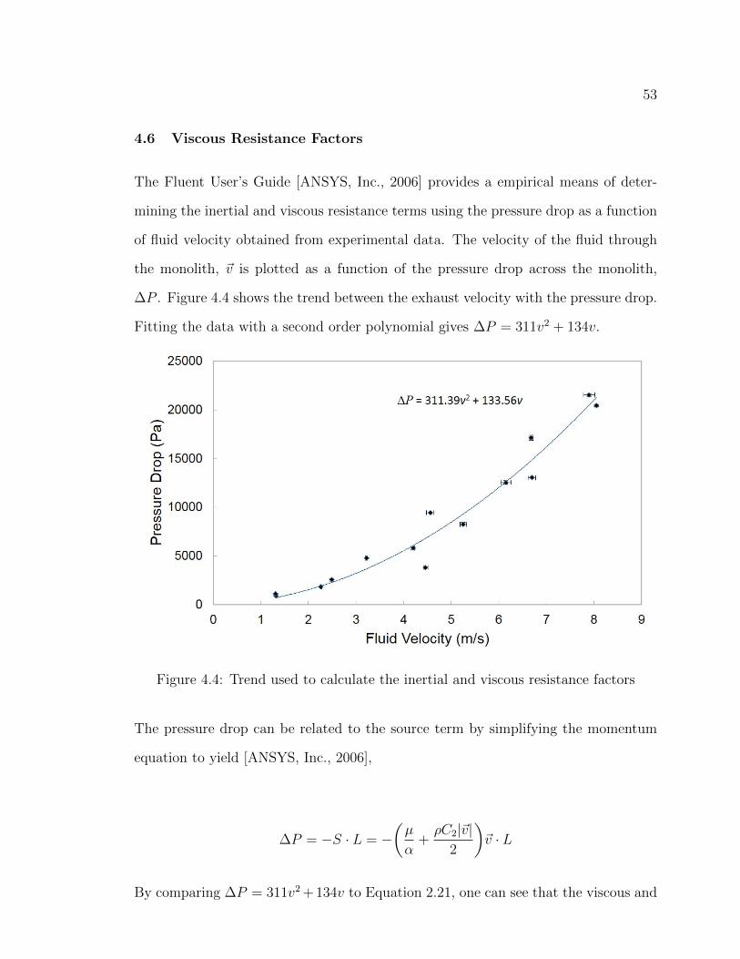
53

4.6 Viscous Resistance Factors

The Fluent User’s Guide [ANSYS, Inc., 2006] provides a empirical means of deter-

mining the inertial and viscous resistance terms using the pressure drop as a function

of fluid velocity obtained from experimental data. The velocity of the fluid through

the monolith, ~v is plotted as a function of the pressure drop across the monolith,

∆P . Figure 4.4 shows the trend between the exhaust velocity with the pressure drop.

Fitting the data with a second order polynomial gives ∆P = 311v2 + 134v.

Figure 4.4: Trend used to calculate the inertial and viscous resistance factors

The pressure drop can be related to the source term by simplifying the momentum

equation to yield [ANSYS, Inc., 2006],

∆P = −S · L = −(µ

α+ρC2|~v|

2

)~v · L

By comparing ∆P = 311v2 + 134v to Equation 2.21, one can see that the viscous and

54

inertial resistance terms can be calculated by observing the following relationships

[ANSYS, Inc., 2006],

134v =µ

αvL (4.3)

311v2 =ρC2

2v2L (4.4)

however it is typically assumed that the inertial resistance factor should be zero (see

Section 6.1.3). Because the experimental results include the pressure drop due to

turbulence in the inlet diffuser and outlet nozzle, and viscous effects from the inlet

and outlet pipes, the inertial resistance factor won’t be zero as the flow is not strictly

laminar in these sections. To correct for the location of the pressure differential

sensors, pressure drop data was collected for the DOC with no monolith with the

results being subtracted from the DOC containing a monolith. Figure 4.5 shows

the results of subtracting the two pressure drop results and indicates a linear trend

between the fluid velocity and pressure drop.

The linear trend between the fluid velocity and pressure drop suggests that the

assumption of negligible inertial resistance in the monolith is valid. Because the

removal of the monolith has a greater effect on the system then just removing the

viscous resistance due to the monolith, the results are not exact but provide an

estimate. Using Equation 2.21 and setting the inertial resistance factor to zero, the

viscous resistance can be found to be 2.2(10)8m−2. Using this value for the viscous

resistance, the numerical analysis returns a pressure drop of 24.6 kPa, larger than

the experimental pressure drop of approximately 12.4 ± 0.4 kPa, giving a relative

difference between the experimental simulation pressure differential of 50%.

The pressure drop across the monolith can be calculated using Poisseuille’s law,

55

Figure 4.5: Trend used to calculate the viscous resistance factor

Equation 2.19. Combining Equation 2.19 and Equation 2.21 and using the average

velocity of exhaust passing through the monolith, the viscous resistance factor can be

found to be 2.2(10)7m−2. This value for the viscous resistance factor gives a differen-

tial pressure across the DOC of 18.9 kPa compared to the experimental differential

pressure of 12.4 ± 0.4 kPa. A relative difference of 34% between the simulation and

experimental pressure differential is much larger than desired however attempts to

increase the accuracy of the pressure drop resulted in abnormal flows through the

DOC and negatively affected the temperature profile.

The difference in pressure drop between the numerical model and the experimental

results can be attributed to the complex flows in the inlet diffuser not being accurately

captured by the numerical model. Furthermore, the monolith is being approximated

as a porous region and this approximation is likely to introduce error that could

reduce the accuracy of the model. To increase the accuracy of the model, more

complex models need to be employed to determine the flow characteristics through

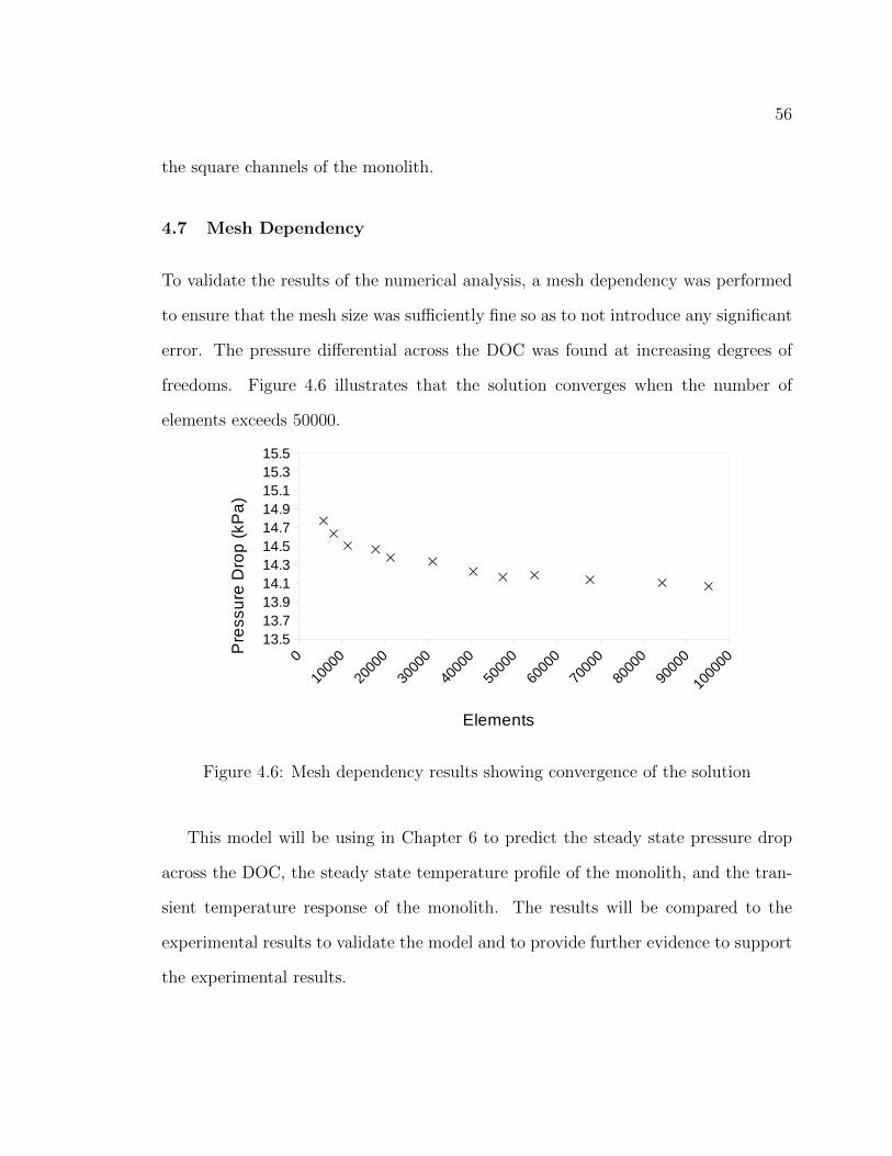
56

the square channels of the monolith.

4.7 Mesh Dependency

To validate the results of the numerical analysis, a mesh dependency was performed

to ensure that the mesh size was sufficiently fine so as to not introduce any significant

error. The pressure differential across the DOC was found at increasing degrees of

freedoms. Figure 4.6 illustrates that the solution converges when the number of

elements exceeds 50000.

Figure 4.6: Mesh dependency results showing convergence of the solution

This model will be using in Chapter 6 to predict the steady state pressure drop

across the DOC, the steady state temperature profile of the monolith, and the tran-

sient temperature response of the monolith. The results will be compared to the

experimental results to validate the model and to provide further evidence to support

the experimental results.

57

Chapter 5

Experimental Flow Characterization

This Chapter details the flow characteristics through the Diesel Oxidation Catalyst

and the temperature characteristics of the Diesel Oxidation Catalyst during heating

and cooling.

5.1 Steady State Pressure Drop

Engine tests were carried out to determine what effect adding an insulation ring to

the monolith of the DOC would have on the overall pressure drop and the radial

temperature profile. It is hypothesized that the insulation ring decreases the pressure

drop by reducing the turbulence in the inlet diffuser and outlet nozzle while main-

taining a higher temperature in the monolith leading to faster light-off. The greatest

reduction in pressure drop is expected for the insulation ring diameter similar to the

inlet diameter of the diffuser which aids in maintaining a jet passing through the

central portion of the DOC and limiting the turbulence in the inlet diffuser. The

pressure drop across the DOC is measured for each of the four DOCs described in

Section 3.5 and at each of the operating points listed in Section 3.7.

Steady state operation is achieved when the exhaust temperature downstream of

the DOC reaches a constant value ±1◦C. The differential pressure across the DOC is

sampled at 1 Hz with the pressure drop calculated as the mean over the subsequent

58

10 seconds. Each test is repeated six times for each of the 14 operating points and for

each of the four DOCs. Since the engine speed can not be precisely controlled and the

stock engine controller makes continuous adjustments, the pressure drop is plotted as

a function of the exhaust volumetric flow rate. The uncertainty in the pressure drop

and flow rate are calculated using a t-distribution with a 95% confidence interval.

Figure 5.1: Pressure drop for each of the four DOCs connected to the Diesel engine

Figure 5.1 indicates that any effect the insulation ring may have on the overall

pressure drop across the DOC is too small to be statistically significant. Pulsations

in the exhaust flow, created by the opening and closing of the exhaust valves and con-

tinuous changes made by the stock engine controller mask any differences in pressure

drop between the various insulation ring sizes.

To eliminate the instabilities caused by the engine, a blower was connected in

place of the Diesel engine. A pitot tube is installed upstream of the DOC to measure

the flow rate of air and the blower is operated at a constant flow rate of 215 ± 4 cfm.

Each of the four insulation rings were tested to determine whether the cold flow tests

using the blower would demonstrate any difference in pressure drop.

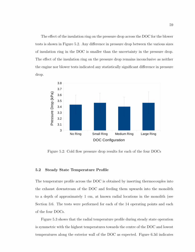
59

The effect of the insulation ring on the pressure drop across the DOC for the blower

tests is shown in Figure 5.2. Any difference in pressure drop between the various sizes

of insulation ring in the DOC is smaller than the uncertainty in the pressure drop.

The effect of the insulation ring on the pressure drop remains inconclusive as neither

the engine nor blower tests indicated any statistically significant difference in pressure

drop.

Figure 5.2: Cold flow pressure drop results for each of the four DOCs

5.2 Steady State Temperature Profile

The temperature profile across the DOC is obtained by inserting thermocouples into

the exhaust downstream of the DOC and feeding them upwards into the monolith

to a depth of approximately 1 cm, at known radial locations in the monolith (see

Section 3.6. The tests were performed for each of the 14 operating points and each

of the four DOCs.

Figure 5.3 shows that the radial temperature profile during steady state operation

is symmetric with the highest temperatures towards the centre of the DOC and lowest

temperatures along the exterior wall of the DOC as expected. Figure 6.3d indicates

60

that the temperature around the centre of the DOC with the large insulation ring

tends to plateau rather then having a defined peak, suggesting that the insulation

ring acts to retain energy at the centre of the DOC.

(a) No Insulation Ring

(b) Small Ring at r = 20.5-23 mm

61

(c) Medium Ring at r = 32.5-35 mm

(d) Large Ring at r = 49.5-52 mm

Figure 5.3: Radial temperature profile of the downstream side of the DOC monolith

The maximum temperature achieved by the DOC during steady state testing is

shown in Figure 5.4. Each of the four DOCs containing different sized insulation rings

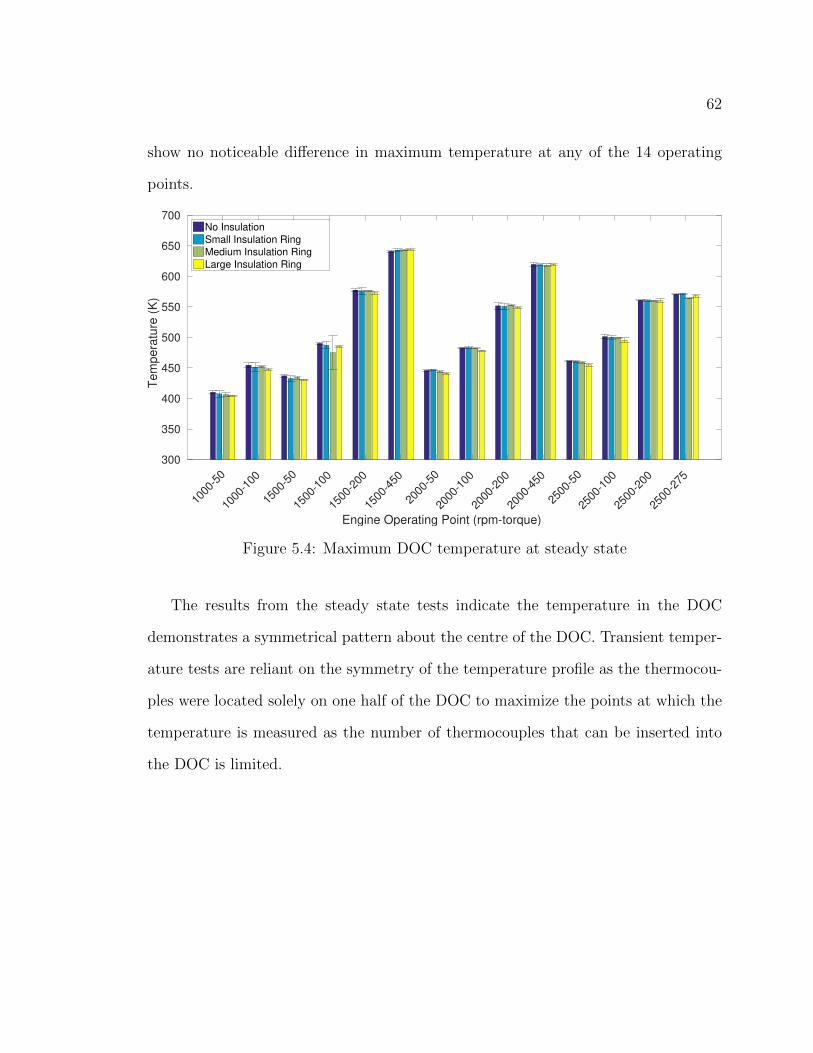
62

show no noticeable difference in maximum temperature at any of the 14 operating

points.

1000

-50

1000

-100

1500

-50

1500

-100

1500

-200

1500

-450

2000

-50

2000

-100

2000

-200

2000

-450

2500

-50

2500

-100

2500

-200

2500

-275

Engine Operating Point (rpm-torque)

300

350

400

450

500

550

600

650

700

Tem

pera

ture

(K

)

No Insulation

Small Insulation Ring

Medium Insulation Ring

Large Insulation Ring

Figure 5.4: Maximum DOC temperature at steady state

The results from the steady state tests indicate the temperature in the DOC

demonstrates a symmetrical pattern about the centre of the DOC. Transient temper-

ature tests are reliant on the symmetry of the temperature profile as the thermocou-

ples were located solely on one half of the DOC to maximize the points at which the

temperature is measured as the number of thermocouples that can be inserted into

the DOC is limited.

63

5.3 Transient Temperature Profile

The temperature profile of each of the four DOCs is recorded as a function of time

for each of the 14 operating points. The temperature of the DOC is recorded on the

downstream side of the monolith at 11 radial locations, located along one half of the

DOC. The thermocouples are inserted approximately 1 cm into the monolith at known

radial locations, as described in Section 3.6, so that the thermocouple’s locations are

the same for all of the tests. The steady state tests in Section 6.1.4 indicated that

the temperature profile is symmetric and it is assumed that a symmetric profile will

occur for the transient tests, allowing all thermocouples to be placed on one half of

the DOC.

0 50 100 150 200 250 300 350 400

Time (s)

280

300

320

340

360

380

400

420

440

Tem

pera

ture

(K

)

Thermocouple 1 (r=0)

Thermocouple 2

Thermocouple 3

Thermocouple 4

Thermocouple 5

Thermocouple 6

Thermocouple 7

Thermocouple 8

Thermocouple 9

Thermocouple 10

Thermocouple 11 (r=90mm)

(a) No Insulation Ring

64

0 100 200 300 400 500

Time (s)

280

300

320

340

360

380

400

420

440

Tem

pera

ture

(K

)

Thermocouple 1 (r=0)

Thermocouple 2

Thermocouple 3

Thermocouple 4

Thermocouple 5

Thermocouple 6

Thermocouple 7

Thermocouple 8

Thermocouple 9

Thermocouple 10

Thermocouple 11 (r=90mm)

(b) Small Ring at r = 20.5-23 mm

0 100 200 300 400 500

Time (s)

300

320

340

360

380

400

420

440

Tem

pera

ture

(K

)

Thermocouple 1 (r=0)

Thermocouple 2

Thermocouple 3

Thermocouple 4

Thermocouple 5

Thermocouple 6

Thermocouple 7

Thermocouple 8

Thermocouple 9

Thermocouple 10

Thermocouple 11 (r=90mm)

(c) Medium Ring at r = 32.5-35 mm

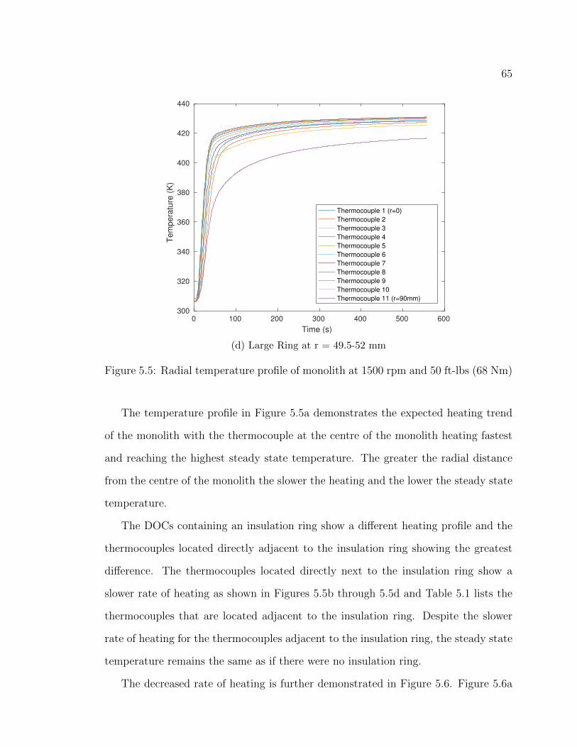
65

0 100 200 300 400 500 600

Time (s)

300

320

340

360

380

400

420

440

Tem

pera

ture

(K

)

Thermocouple 1 (r=0)

Thermocouple 2

Thermocouple 3

Thermocouple 4

Thermocouple 5

Thermocouple 6

Thermocouple 7

Thermocouple 8

Thermocouple 9

Thermocouple 10

Thermocouple 11 (r=90mm)

(d) Large Ring at r = 49.5-52 mm

Figure 5.5: Radial temperature profile of monolith at 1500 rpm and 50 ft-lbs (68 Nm)

The temperature profile in Figure 5.5a demonstrates the expected heating trend

of the monolith with the thermocouple at the centre of the monolith heating fastest

and reaching the highest steady state temperature. The greater the radial distance

from the centre of the monolith the slower the heating and the lower the steady state

temperature.

The DOCs containing an insulation ring show a different heating profile and the

thermocouples located directly adjacent to the insulation ring showing the greatest

difference. The thermocouples located directly next to the insulation ring show a

slower rate of heating as shown in Figures 5.5b through 5.5d and Table 5.1 lists the

thermocouples that are located adjacent to the insulation ring. Despite the slower

rate of heating for the thermocouples adjacent to the insulation ring, the steady state

temperature remains the same as if there were no insulation ring.

The decreased rate of heating is further demonstrated in Figure 5.6. Figure 5.6a

66

Table 5.1: List of thermocouples located next to the insulation ring

DOC Configuration ThermocoupleSmall Insulation Ring (Figure 5.3b) 2 and 3Medium Insulation Ring (Figure 5.3c) 5 and 6Large Insulation Ring (Figure 6.3d) 9 and 10

shows that the rate of DOC heating does not decrease uniformly from the centre of

the DOC to the wall of the DOC but rather the rate of heating occurs fastest at

the centre of the DOC and approximately 30 mm from the centre of the DOC. This

suggests that there is a larger flow rate of exhaust passing through these two locations

of the DOC and increasing the amount of available energy. The increased flow rate at

approximately 30 mm corresponds to the inlet diameter of the diffuser and is likely a

result of the turbulent flow into the monolith.

0 20 40 60 80

Radial Position (mm)

275

300

325

350

375

400

425

450

Tem

pera

ture

(K

)

t=50

t=45

t=40

t=35

t=30

t=25

t=20

t=15

t=10

t=5

t=1

(a) No Insulation Ring

67

0 20 40 60 80

Radial Position (mm)

275

300

325

350

375

400

425

450

Tem

pera

ture

(K

)

t=50

t=45

t=40

t=35

t=30

t=25

t=20

t=15

t=10

t=5

t=1

(b) Small Ring at r = 20.5-23 mm

0 20 40 60 80

Radial Position (mm)

275

300

325

350

375

400

425

450

Te

mp

era

ture

(K

)

t=50

t=45

t=40

t=35

t=30

t=25

t=20

t=15

t=10

t=5

t=1

(c) Medium Ring at r = 32.5-35 mm

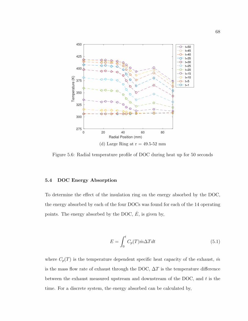
68

0 20 40 60 80

Radial Position (mm)

275

300

325

350

375

400

425

450

Tem

pera

ture

(K

)

t=50

t=45

t=40

t=35

t=30

t=25

t=20

t=15

t=10

t=5

t=1

(d) Large Ring at r = 49.5-52 mm

Figure 5.6: Radial temperature profile of DOC during heat up for 50 seconds

5.4 DOC Energy Absorption

To determine the effect of the insulation ring on the energy absorbed by the DOC,

the energy absorbed by each of the four DOCs was found for each of the 14 operating

points. The energy absorbed by the DOC, E, is given by,

E =

∫ t

0

Cp(T )m∆Tdt (5.1)

where Cp(T ) is the temperature dependent specific heat capacity of the exhaust, m

is the mass flow rate of exhaust through the DOC, ∆T is the temperature difference

between the exhaust measured upstream and downstream of the DOC, and t is the

time. For a discrete system, the energy absorbed can be calculated by,

69

E =t∑0

Cp(T )m∆T∆t (5.2)

where ∆t is the sampling step size. The specific heat capacity of the exhaust is

approximated using the specific heat of air and calculated using the following [Cengel

and Boles, 2011],

Cp(T ) = a+ bT + cT 2 + dT 3 (kJ/(kmol-K)) (5.3)

where the coefficients in Equation 5.3 are given as [Cengel and Boles, 2011]:

Table 5.2: Coefficients used to calculate Cp(T )

Coefficient Valuea 28.11b 0.1967(10)−2

c 0.4802(10)−5

d −1.966(10)−9

Energy transfer from the DOC to the surroundings is calculated by determining

the rate of energy absorption by the DOC at steady state since the energy absorbed

by the DOC at steady state is equal to the energy lost to the surroundings. To

calculate the energy transfer to the surroundings during the transient phase, a linear

interpolation is used to give an approximate rate of energy transfer. Because the rate

of energy transfer to the surroundings is not linear with temperature, some degree

of error is introduced, but because the rate of heating is approximately the same for

each of the four DOCs for the same operating point, the relative difference between

the DOCs can be compared.

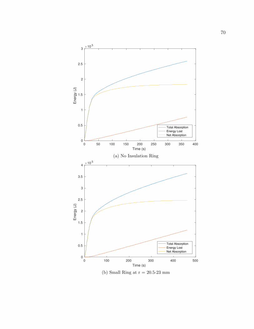
70

0 50 100 150 200 250 300 350 400

Time (s)

0

0.5

1

1.5

2

2.5

3

En

erg

y (

J)

×10 5

Total Absorption

Energy Lost

Net Absorption

(a) No Insulation Ring

0 100 200 300 400 500

Time (s)

0

0.5

1

1.5

2

2.5

3

3.5

4

En

erg

y (

J)

×10 5

Total Absorption

Energy Lost

Net Absorption

(b) Small Ring at r = 20.5-23 mm

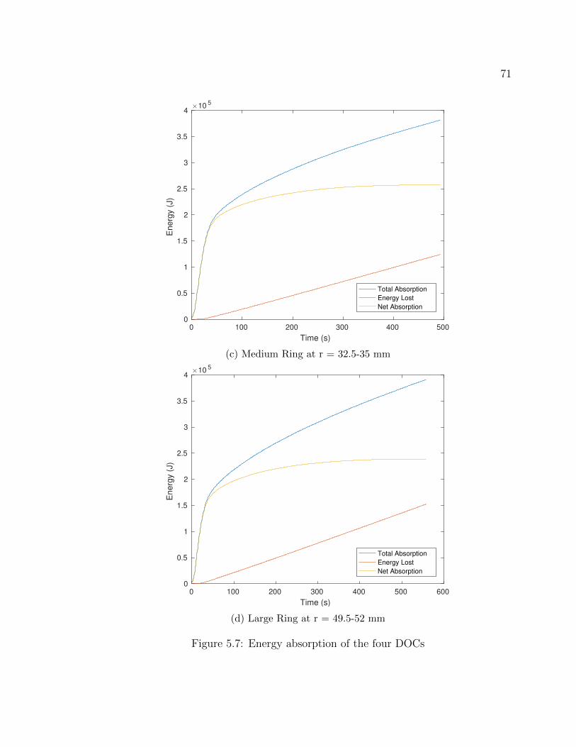
71

0 100 200 300 400 500

Time (s)

0

0.5

1

1.5

2

2.5

3

3.5

4

En

erg

y (

J)

×10 5

Total Absorption

Energy Lost

Net Absorption

(c) Medium Ring at r = 32.5-35 mm

0 100 200 300 400 500 600

Time (s)

0

0.5

1

1.5

2

2.5

3

3.5

4

En

erg

y (

J)

×10 5

Total Absorption

Energy Lost

Net Absorption

(d) Large Ring at r = 49.5-52 mm

Figure 5.7: Energy absorption of the four DOCs

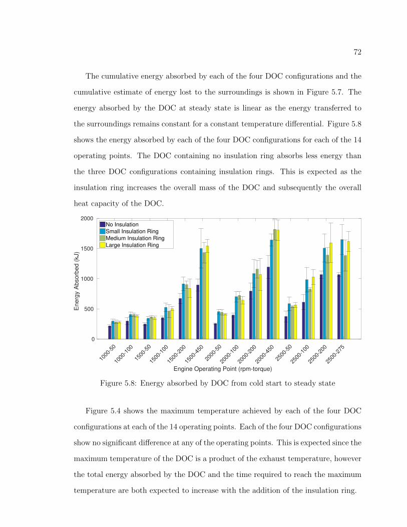
72

The cumulative energy absorbed by each of the four DOC configurations and the

cumulative estimate of energy lost to the surroundings is shown in Figure 5.7. The

energy absorbed by the DOC at steady state is linear as the energy transferred to

the surroundings remains constant for a constant temperature differential. Figure 5.8

shows the energy absorbed by each of the four DOC configurations for each of the 14

operating points. The DOC containing no insulation ring absorbs less energy than

the three DOC configurations containing insulation rings. This is expected as the

insulation ring increases the overall mass of the DOC and subsequently the overall

heat capacity of the DOC.

1000

-50

1000

-100

1500

-50

1500

-100

1500

-200

1500

-450

2000

-50

2000

-100

2000

-200

2000

-450

2500

-50

2500

-100

2500

-200

2500

-275

Engine Operating Point (rpm-torque)

0

500

1000

1500

2000

Energ

y A

bsorb

ed (

kJ)

No Insulation

Small Insulation Ring

Medium Insulation Ring

Large Insulation Ring

Figure 5.8: Energy absorbed by DOC from cold start to steady state

Figure 5.4 shows the maximum temperature achieved by each of the four DOC

configurations at each of the 14 operating points. Each of the four DOC configurations

show no significant difference at any of the operating points. This is expected since the

maximum temperature of the DOC is a product of the exhaust temperature, however

the total energy absorbed by the DOC and the time required to reach the maximum

temperature are both expected to increase with the addition of the insulation ring.

73

Figure 5.9a indicates that the time to reach 95% of the steady state temperature

is greater for the three DOC configurations containing an insulation ring. Further-

more, Figures 5.9b through 5.9d illustrate that the time required to reach 85%, 75%,

and 50% the steady state temperature are even greater for the DOC configurations

containing insulation rings. The delay in heating of the DOC is likely to negatively

affect the light-off characteristics of the DOC.

1000

-50

1000

-100

1500

-50

1500

-100

1500

-200

1500

-450

2000

-50

2000

-100

2000

-200

2000

-450

2500

-50

2500

-100

2500

-200

2500

-275

Engine Operating Point (rpm-torque)

0

50

100

150

200

Tim

e (

s)

No Insulation

Small Insulation Ring

Medium Insulation Ring

Large Insulation Ring

(a) Time required for DOC to reach 95% of steady state temperature

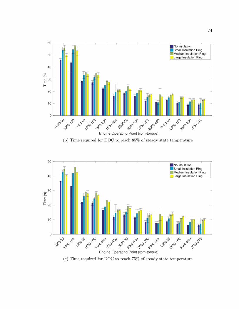
74

1000

-50

1000

-100

1500

-50

1500

-100

1500

-200

1500

-450

2000

-50

2000

-100

2000

-200

2000

-450

2500

-50

2500

-100

2500

-200

2500

-275

Engine Operating Point (rpm-torque)

0

10

20

30

40

50

60T

ime (

s)

No Insulation

Small Insulation Ring

Medium Insulation Ring

Large Insulation Ring

(b) Time required for DOC to reach 85% of steady state temperature

1000

-50

1000

-100

1500

-50

1500

-100

1500

-200

1500

-450

2000

-50

2000

-100

2000

-200

2000

-450

2500

-50

2500

-100

2500

-200

2500

-275

Engine Operating Point (rpm-torque)

0

10

20

30

40

50

Tim

e (

s)

No Insulation

Small Insulation Ring

Medium Insulation Ring

Large Insulation Ring

(c) Time required for DOC to reach 75% of steady state temperature

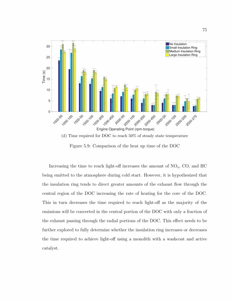
75

1000

-50

1000

-100

1500

-50

1500

-100

1500

-200

1500

-450

2000

-50

2000

-100

2000

-200

2000

-450

2500

-50

2500

-100

2500

-200

2500

-275

Engine Operating Point (rpm-torque)

0

5

10

15

20

25

30T

ime (

s)

No Insulation

Small Insulation Ring

Medium Insulation Ring

Large Insulation Ring

(d) Time required for DOC to reach 50% of steady state temperature

Figure 5.9: Comparison of the heat up time of the DOC

Increasing the time to reach light-off increases the amount of NOx, CO, and HC

being emitted to the atmosphere during cold start. However, it is hypothesized that

the insulation ring tends to direct greater amounts of the exhaust flow through the

central region of the DOC increasing the rate of heating for the core of the DOC.

This in turn decreases the time required to reach light-off as the majority of the

emissions will be converted in the central portion of the DOC with only a fraction of

the exhaust passing through the radial portions of the DOC. This effect needs to be

further explored to fully determine whether the insulation ring increases or decreases

the time required to achieve light-off using a monolith with a washcoat and active

catalyst.

76

5.5 Experimental Limitations

The experimental setup demonstrated a number of drawbacks that limited the conclu-

sions that could be formed and will be outlined for future work along with suggested

changes. By improving the current experimental setup, future work will be able to

draw more definitive conclusions.

The exhaust bypass described in Section 3.4 allows the engine to be warmed to

steady state without heating the DOC. When the engine reaches steady state the

exhaust valve to the DOC can be opened and the bypass closed. The intended

purpose is to creating a step input in the exhaust gas temperature passing through

the DOC. The valves were only partially capable of isolating heat transfer to the DOC

as under high temperatures (600 K) and high exhaust flow rates (200 g/s) the valves

would not seal completely. Although this had little effect on steady state testing, the

uncertainty in the transient test results was adversely affected. Valves used for the

exhaust bypass should be intended for high temperature application but also be able

to handle large variations in temperature (300 K to 600 K).

Pulsations in the exhaust gas occurring due to the opening and closing of the

exhaust valves and automatic changes made by the stock engine controller increases

the uncertainty in the exhaust gas flow rate. In order to reduce the pulsations it has

been suggested that multiple blank catalysts can be used upstream to dampen the

pulsations or a hot flow bench with a constant flow rate can be used in place of the

engine.

77

Chapter 6

Simulation Based Flow Characterization

This Chapter details the results of the numerical analysis to define the flow character-

istics through the Diesel Oxidation Catalyst, including the pressure drop and heating

characteristics. Both steady state and transient numerical models are discussed.

6.1 Steady State Numerical Model

The addition of an insulation ring to the monolith of the DOC is examined to de-

termine if there exists a difference in the overall pressure drop across the DOC and

whether the temperature profile is affected. By reducing the pressure drop across

the DOC the back pressure on the engine can be reduced leading to increased engine

efficiency.

6.1.1 Steady State Setup

The model is setup using an exhaust flow rate of 175 g/s, similar to the exhaust flow

rate from the Cummins QSB4.5 Diesel engine at 1500 rpm and 610 N/m (450 ft-

lbs) (see Section 3.2). The pulsations that occur in the exhaust due to the opening

and closing of the exhaust valves are ignored to simplify the numerical model. The

monolith is modeled as a porous region with axial flow being imposed by setting

the viscous resistance value in the radial direction to a minimum of three orders of

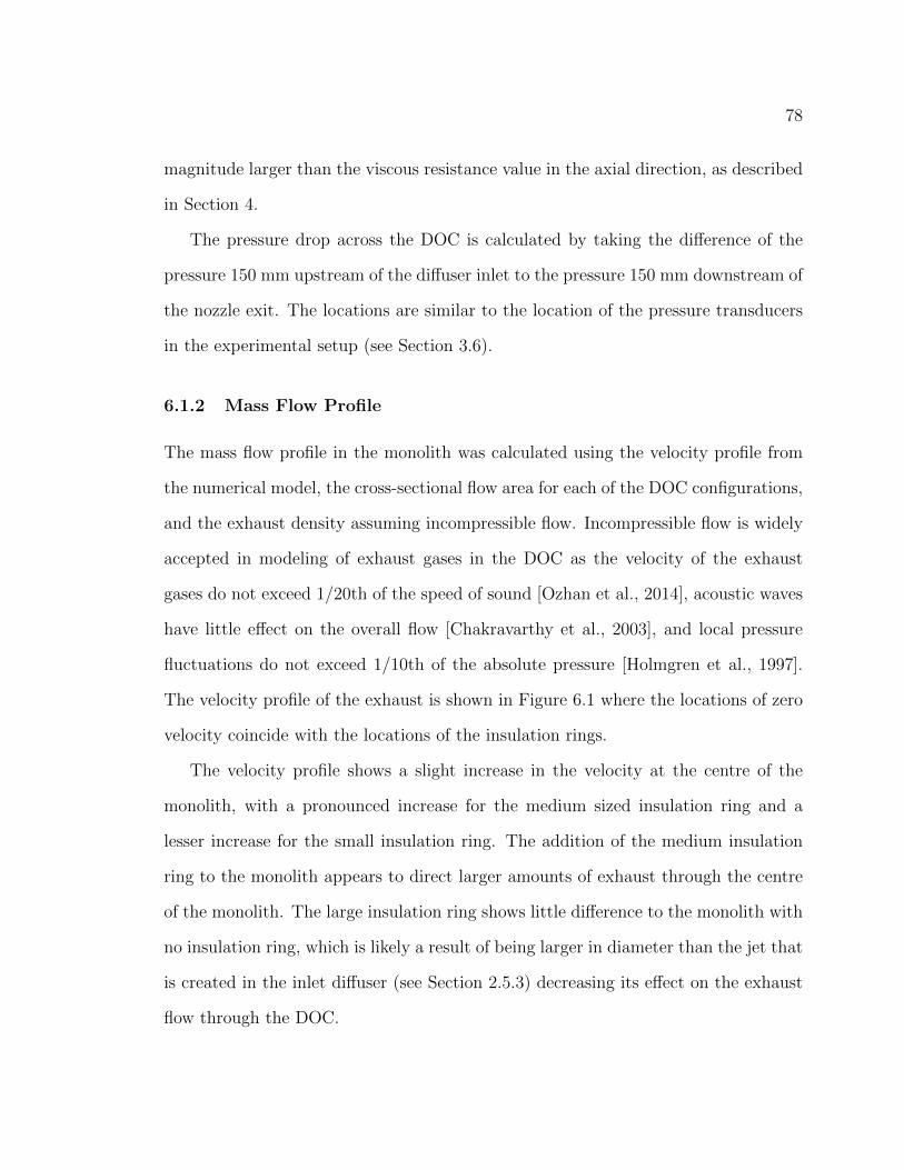
78

magnitude larger than the viscous resistance value in the axial direction, as described

in Section 4.

The pressure drop across the DOC is calculated by taking the difference of the

pressure 150 mm upstream of the diffuser inlet to the pressure 150 mm downstream of

the nozzle exit. The locations are similar to the location of the pressure transducers

in the experimental setup (see Section 3.6).

6.1.2 Mass Flow Profile

The mass flow profile in the monolith was calculated using the velocity profile from

the numerical model, the cross-sectional flow area for each of the DOC configurations,

and the exhaust density assuming incompressible flow. Incompressible flow is widely

accepted in modeling of exhaust gases in the DOC as the velocity of the exhaust

gases do not exceed 1/20th of the speed of sound [Ozhan et al., 2014], acoustic waves

have little effect on the overall flow [Chakravarthy et al., 2003], and local pressure

fluctuations do not exceed 1/10th of the absolute pressure [Holmgren et al., 1997].

The velocity profile of the exhaust is shown in Figure 6.1 where the locations of zero

velocity coincide with the locations of the insulation rings.

The velocity profile shows a slight increase in the velocity at the centre of the

monolith, with a pronounced increase for the medium sized insulation ring and a

lesser increase for the small insulation ring. The addition of the medium insulation

ring to the monolith appears to direct larger amounts of exhaust through the centre

of the monolith. The large insulation ring shows little difference to the monolith with

no insulation ring, which is likely a result of being larger in diameter than the jet that

is created in the inlet diffuser (see Section 2.5.3) decreasing its effect on the exhaust

flow through the DOC.

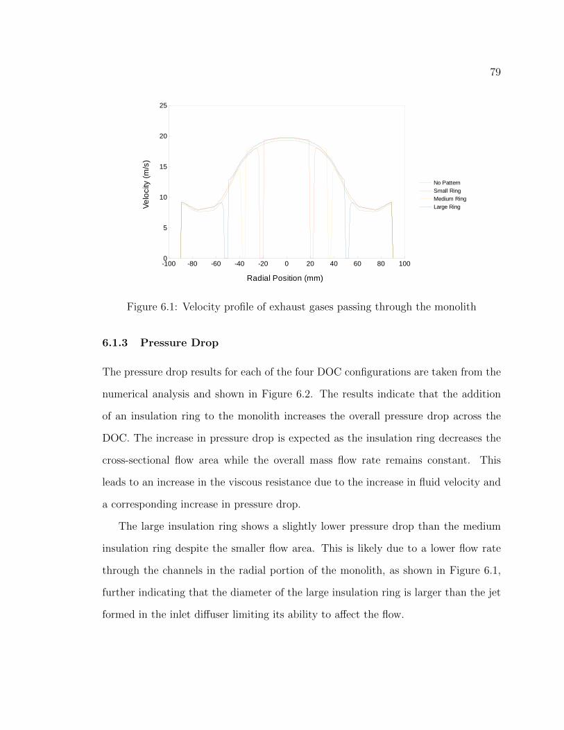
79

Figure 6.1: Velocity profile of exhaust gases passing through the monolith

6.1.3 Pressure Drop

The pressure drop results for each of the four DOC configurations are taken from the

numerical analysis and shown in Figure 6.2. The results indicate that the addition

of an insulation ring to the monolith increases the overall pressure drop across the

DOC. The increase in pressure drop is expected as the insulation ring decreases the

cross-sectional flow area while the overall mass flow rate remains constant. This

leads to an increase in the viscous resistance due to the increase in fluid velocity and

a corresponding increase in pressure drop.

The large insulation ring shows a slightly lower pressure drop than the medium

insulation ring despite the smaller flow area. This is likely due to a lower flow rate

through the channels in the radial portion of the monolith, as shown in Figure 6.1,

further indicating that the diameter of the large insulation ring is larger than the jet

formed in the inlet diffuser limiting its ability to affect the flow.

80

Figure 6.2: Pressure drop across the DOC for each of the DOC configurations

6.1.4 Steady State Temperature Profile

The temperature profile was found 1 cm upstream from the downstream face of the

monolith, similar to the location of the thermocouples in the experimental tests,

allowing the results to be easily compared (see Section 3.6). The parameters used in

the numerical analysis are found in Chapter 4.

The steady state temperature profile was plotted along with the experimental

temperature data for the operating point of 1950 rpm and 200 ft-lbs, which produces

an exhaust flow rate of 0.18 ± 0.03 kg/s, similar to the flow rate of 0.175 kg/s used

by the numerical model. Figure 6.3 illustrates the ability of the numerical model to

accurately predict the temperature profile of the monolith.

81

(a) No Insulation Ring

(b) Small Ring at r = 20.5-23 mm

82

(c) Medium Ring at r = 32.5-35 mm

(d) Large Ring at r = 49.5-52 mm

Figure 6.3: Radial temperature profile of the downstream side of the DOC monolith

Comparing the steady state temperature profiles of the four DOC configurations,

shown in Figure 6.4, it can be seen that the insulation ring increases the temperature

of the monolith 50 to 75 mm from the centre of the monolith without decreasing the

temperature at the centre of the DOC. The higher temperature in the radial portions

of the DOC due to the addition of the insulation ring illustrates the ability of the

83

insulation ring to reduce the heat transfer from the DOC. Reducing the heat transfer

from the DOC and maintaining a higher temperature towards the centre of monolith

will help improve the light-off characteristics of the DOC during low load operation

or periods of time when the engine is turned off for short time intervals. With

vehicles automatically stopping the engine whenever the vehicle stops, maintaining

the catalyst above the light-off for longer will decrease the overall emissions produced.

Figure 6.4: Monolith temperature profile for each of the four DOC configurations

6.2 Transient Numerical Model

The heating characteristics of the DOC were examined by developing a numerical

model with a step in the temperature input. This section details the time-dependent

temperature input and the ability of the numerical model to predict the DOC tem-

perature response.

6.2.1 Temperature Input

The setup of the numerical analysis used the same parameters as the steady state

analysis with the exception of the inlet temperature, which was varied using a user-

84

defined variable input temperature. The following sigmoidal function was used,

Tinlet =

288 K + 300 K 1

1+2.2−t+5 t ≤ 20 s

590 K t > 20 s

(6.1)

where Tinlet is the exhaust inlet temperature in Kelvin and t is the time step in

seconds. The inlet temperature starts at 303 K and increases to 590 K in the first

20 time steps and then remains constant at 590 K for the remaining time steps, as

shown in Figure 6.5, and is compared with the experimental step in inlet temperature

measured just upstream of the DOC for the operating point 1950 rpm and 450 ft-lbs

for a flow rate of 176.0 ± 25.5 g/s (see Section 3.6).

Figure 6.5: Inlet temperature of the exhaust gas used in the numerical analysis

6.2.2 Transient Model Validation

The heating characteristics predicted by the numerical model for each of the four DOC

configurations are shown in Figures 6.6. The heating profile demonstrates that the

DOC undergoes the highest rate of temperature increase at the centre of the monolith

with the rate of heating decaying with increasing radial distance. The insulating ring

reduces the rate of heating adjacent to the ring and shown in Figures 6.6b to 6.6d. The

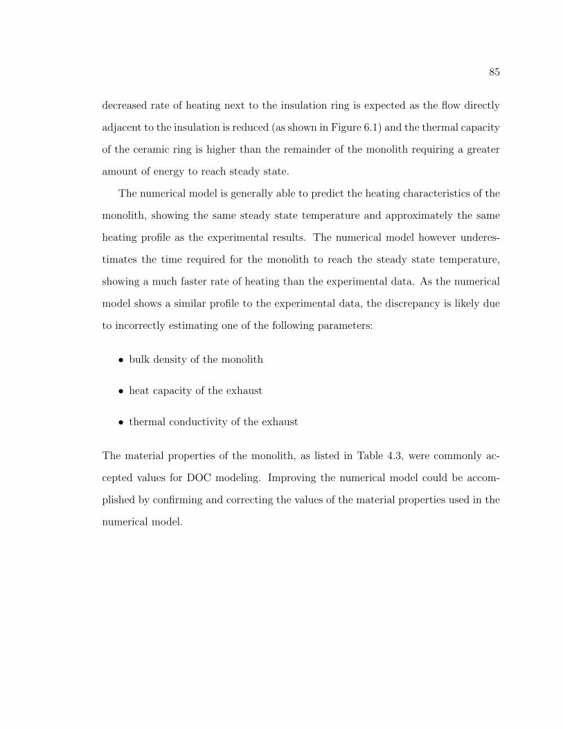
85

decreased rate of heating next to the insulation ring is expected as the flow directly

adjacent to the insulation is reduced (as shown in Figure 6.1) and the thermal capacity

of the ceramic ring is higher than the remainder of the monolith requiring a greater

amount of energy to reach steady state.

The numerical model is generally able to predict the heating characteristics of the

monolith, showing the same steady state temperature and approximately the same

heating profile as the experimental results. The numerical model however underes-

timates the time required for the monolith to reach the steady state temperature,

showing a much faster rate of heating than the experimental data. As the numerical

model shows a similar profile to the experimental data, the discrepancy is likely due

to incorrectly estimating one of the following parameters:

• bulk density of the monolith

• heat capacity of the exhaust

• thermal conductivity of the exhaust

The material properties of the monolith, as listed in Table 4.3, were commonly ac-

cepted values for DOC modeling. Improving the numerical model could be accom-

plished by confirming and correcting the values of the material properties used in the

numerical model.

86

(a) No Insulation Ring

(b) Small Ring at r = 20.5-23 mm

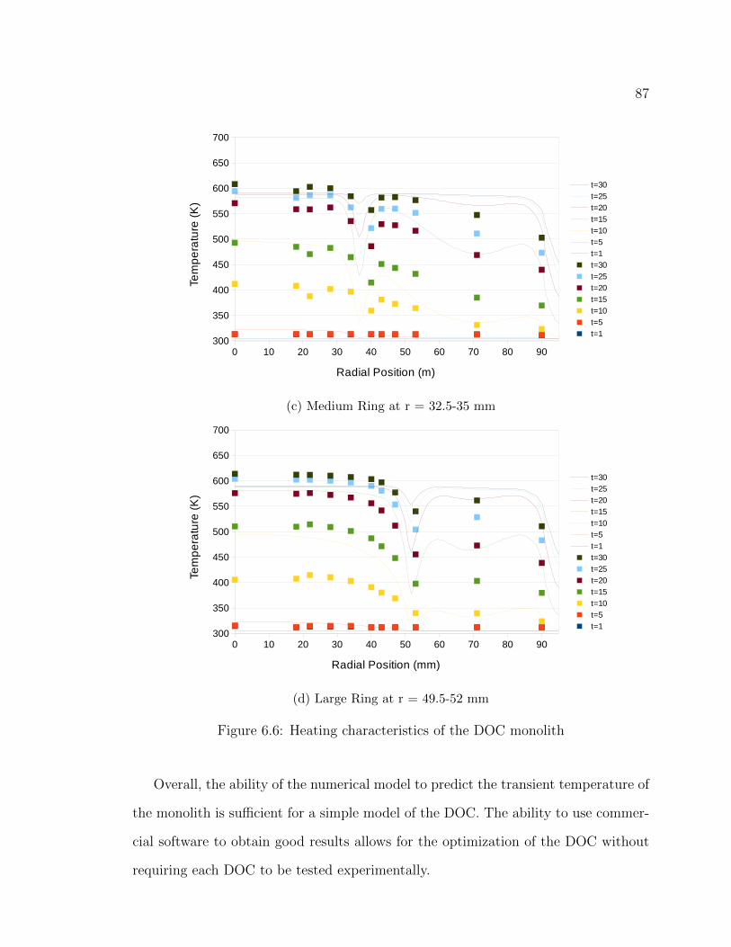
87

(c) Medium Ring at r = 32.5-35 mm

(d) Large Ring at r = 49.5-52 mm

Figure 6.6: Heating characteristics of the DOC monolith

Overall, the ability of the numerical model to predict the transient temperature of

the monolith is sufficient for a simple model of the DOC. The ability to use commer-

cial software to obtain good results allows for the optimization of the DOC without

requiring each DOC to be tested experimentally.

88

6.2.3 DOC Heating Characteristics

The heating characteristics of each of the four DOC configurations is important in

understanding the effect the insulation ring has on the light-off characteristics. The

heating characteristics of the four DOC configurations are shown in Figure 6.7, com-

paring the temperature of each of the four DOC configurations at 5 s, 10 s, 15 s, and

20 s after the beginning of the step in inlet temperature described in Section 6.2.1.

The addition of an insulation ring shows a reduced temperature adjacent to and

within the insulation ring due to the higher heat capacity of the ceramic requiring a

greater amount of time for the insulation ring to reach the same temperature as the

remainder of the monolith. Despite this decrease in temperature it is interesting to

note that the remainder of the monolith heats at a greater rate if an insulation ring

is present, which can be seen in both Figures 6.7b and 6.7c.

An increase in the rate of heating due to the addition of an insulating ring occurs

at both the centre and radial portions of the DOC. The center of the DOC containing

any of the three sizes of insulation ring reaches a temperature of approximately 4 K

higher than the DOC containing no insulation ring after 10 s of heating (shown in

Figure 6.7b) while the radial portion of the DOC reaches a temperature of up to 20 K

higher after 15 s of heating (Figure 6.7c).

The steady state temperature of the DOC is approximately the same with a small

increase in temperature in the radial portion of the DOC, as discussed in Section 6.1.4.

The temperature of the ceramic ring and the channels directly adjacent however

require a much longer time to reach steady state, which is expected due to the higher

heat capacity of the ceramic ring and the decreased flow adjacent to the ceramic ring

as discussed in Section 6.1.2. The overall ability of the insulation ring to reduce the

light-off time of the monolith when both the increase in heating of the centre and

radial portions of the monolith is combined with the decrease in temperature next to

89

the ceramic ring are combined needs to be further examined.

(a) t = 5 s

(b) t = 10 s

90

(c) t = 15 s

(d) t = 20 s

Figure 6.7: Comparison of the heating characteristics of the four DOC configurations

6.3 Assumptions and Limitations

The numerical model is based on assumptions that allow it to be applied easily. These

simplifications however limit the conditions to which the model can be applied.

91

A limiting assumption used in the numerical model is that the material properties

of the DOC and the exhaust gas were considered constant. This decreases the accu-

racy of the transient numerical model where the temperature varies between 300 and

600 K resulting in material properties that can change by up to 30%. As the material

properties were selected for temperatures between 500 and 600 K, it is important to

understand that the results will be adversely affected by error introduced in assuming

constant properties.

The material properties are estimated using data found in the literature and ap-

proximating the exhaust gases from a Diesel engine as air at the desired temperature.

Determining the exact properties of the monolith is difficult as it is constructed of

extruded cordierite for which the material properties can vary depending on the man-

ufacturing conditions.

The model uses a standard k-omega SST turbulence model and assumes that the

flow through the monolith is laminar. The accuracy of the turbulence model in the

inlet diffuser is currently assumed to be sufficient, however the effects of turbulence

have an effect on the pressure drop and temperature profile in the monolith. De-

termining the accuracy of the turbulence model and the validity of the laminar flow

assumption will further add to the accuracy of the numerical model.

Finally, the monolith in the numerical model does not contain a washcoat or active

catalyst. This allows for optimization of the flow through the catalyst by separating

the effects of the geometry from chemical reactions but limits the numerical model.

Furthermore, the chemical reactions have the ability to change the flow characteristics

by increasing or decreasing the pressure drop as the the exhaust chemical composition

changes.

92

Chapter 7

Conclusions

Conclusions for experimental and numerical results are presented here along with

recommendations for future work is detailed.

7.1 Pressure Drop

The experimental results were unable to show a statistically significant difference in

pressure drop between the DOC without an insulation ring and the DOC configu-

rations containing an insulation ring. Due to the variability of the results, caused

primarily from the pulsations in the exhaust flow, the uncertainty in the pressure

drop was large while the expected differences are expected to be small, as was shown

with the numerical model which indicated a difference of only 1 kPa.

The numerical model was only able to calculate a pressure drop to within 30%

of the experimental pressure drop. The pressure drop is dependent on the viscous

resistance factor as well as the density and viscosity of the exhaust gas. The viscous

resistance was calculated analytically from Poisseuille’s law and provided the best

estimate of the viscous resistance. Despite a larger pressure drop than the experi-

mental results, the numerical model demonstrated that the addition of an insulation

ring tended to increase the pressure drop and captured the same trend as the exper-

iment. The pressure drop was not directly proportional to the decrease in flow area

93

with the large insulation ring showing a lower pressure drop than the medium insu-

lation ring. This is likely due to the lower flow rate through the individual channels

in the radial portions of the monolith.

7.2 Temperature Profile

The steady state temperature profile of the DOC was found experimentally and

showed a symmetrical profile across the monolith. The steady state temperature

showed a decaying temperature profile with the highest temperature found at the

centre of the monolith and the lowest temperature at the wall of the DOC. This is

expected as the highest flow rate of exhaust gases per unit area is expected at the

centre of the monolith and the heat is dissipated at the wall of the DOC. The exper-

imental results indicate that the time required for the monolith to reach its steady

state temperature is increased with the addition of an insulation ring. This has the

potential of increasing the time required by the DOC to reach light-off, increasing the

pollutants emitted.

The numerical model showed a similar profile to the experimental results further

validating the model. The numerical model showed a similar decay in temperature

from the centre of the monolith to the DOC walls, with an increased drop in the

temperature close to the DOC wall. Although the experimental tests indicated that

the addition of an insulation ring increased the time for the DOC to reach steady state,

the numerical model indicated that although true, the increase in time is associated

with the increased time for the ceramic ring to heat to steady state with the remainder

of the monolith heating faster. The benefit of the insulation ring to reducing the time

required for the DOC to reach light-off needs to be determined as there is a decrease

in temperature directly adjacent to the insulation ring which has the potential of

offsetting the benefits.

94

The experimental transient temperature profile showed a non-uniform rate of heat-

ing with two maximums between the centre of the monolith and the wall of the DOC.

The first peak was at the centre of the monolith while the second peak was approx-

imately 30 mm from the centre. The second peak corresponds approximately to the

radius of the inlet to the diffuser and is likely the result of flow maldistribution caused

by the inlet diffuser. The addition of the insulation ring results in a drop in heating

rate adjacent to the insulation ring with the temperature recovering as the monolith

reaches steady state.

The transient numerical model showed similarities to the experimental results

apart from the differences in the rate of heating. The rate of heating in the numerical

model was greater than the experimental results showed and is likely the result of

underestimating the bulk density of the monolith or the heat capacity of the exhaust.

7.3 Insulation Ring

Under the current experimental setup, the results showed no statistical difference in

pressure drop between the DOC configurations as the variation in the data associated

with the setup, primarily from pulsations in the exhaust flow, was greater than the

expected difference in pressure drop. The numerical model indicates that the expected

difference in pressure drop between the DOC configurations is approximately 1 kPa,

with the addition of an insulation ring increasing the pressure drop.

The numerical model indicates the ability of the insulation ring to maintain the

heat within the monolith and decrease the time required to reach light-off. The

increased time for the DOC to reach steady state shown in the experimental tests is

shown by the numerical model to be a result of the insulation ring requiring a greater

time to reach steady state. Although the numerical model indicates that the majority

of the monolith heats faster with the addition of an insulation ring, the area directly

95

adjacent to the insulation ring shows a slower rate of heating. The combined effect

of the slower heating adjacent to the insulation ring and the increased rate of heating

throughout the remainder of the monolith needs to be determined.

7.4 Future Work

• Testing of the four DOC configurations on an improved experimental setup that

eliminates the pressure fluctuations in the exhaust flow to determine the effect

of adding an insulation ring on the pressure drop.

• Determine whether the insulation ring decreases the time required for the DOC

to reach light-off by measuring the exhaust composition after a step in inlet

temperature downstream of the DOC.

• Investigate the differences between various DOC geometries, including the angle

of the inlet diffuser and outlet nozzle.

• Demonstrate that numerical models of the DOC without an active catalyst is a

valid simplification for DOC flow optimization.

• Improvement of the numerical model to the effects of turbulence in the inlet

diffuser and verification of the laminar flow assumption in the monolith.

• Testing of the DOC with an active catalyst to determine the validity of using

models containing no catalyst to characterize the flow of exhaust gases through

the DOC.

96

References

Andersson, B., Andersson, R., Hakansson, L., Mortensen, M., Sudiyo, R., and

Van Wachem, B. (2012). Computational fluid dynamics for engineers. Cambridge

University Press, 1 edition.

Andrews, G. E., Ahamed, F. M., and Li, H. (2007). Condensable and Gaseous Hy-

drocarbon Emissions and Their Speciation for a Real World SI Car Test. Technical

report, SAE Technical Paper.

ANSYS, Inc. (2006). FLUENT 6.3 Users Guide. ANSYS, Inc., 275 Technology Drive,

Canonsburg, PA 15317, 6.3 edition.

Barbosa, F. C. (2016). Heavy Duty Emission Standards Assessment-An Engine and

Aftertreatment Technological Approach. Technical report, SAE Technical Paper.

Bartley, G. J. (2015). Identifying Limiters to Low Temperature Catalyst Activity.

Technical report, SAE Technical Paper.

Bond, T. C. and Bergstrom, R. W. (2006). Light absorption by carbonaceous parti-

cles: An investigative review. Aerosol science and technology, 40(1):27–67.

Bond, T. C., Doherty, S. J., Fahey, D., Forster, P., Berntsen, T., DeAngelo, B.,

Flanner, M., Ghan, S., Karcher, B., Koch, D., et al. (2013). Bounding the role of

black carbon in the climate system: A scientific assessment. Journal of Geophysical

Research: Atmospheres, 118(11):5380–5552.

97

Bowman, C. T. (1975). Kinetics of pollutant formation and destruction in combustion.

Progress in energy and combustion science, 1(1):33–45.

Cappa, C. D., Onasch, T. B., Massoli, P., Worsnop, D. R., Bates, T. S., Cross, E. S.,

Davidovits, P., Hakala, J., Hayden, K. L., Jobson, B. T., et al. (2012). Radiative

absorption enhancements due to the mixing state of atmospheric black carbon.

Science, 337(6098):1078–1081.

Carpenter, L., Clemitshaw, K., Burgess, R., Penkett, S., Cape, J., and McFadyen, G.

(1998). Investigation and evaluation of the NOx/O3 photochemical steady state.

Atmospheric Environment, 32(19):3353–3365.

Cavataio, G., Girard, J., Patterson, J. E., Montreuil, C., Cheng, Y., and Lambert,

C. K. (2007). Laboratory testing of urea-SCR formulations to meet tier 2 bin 5

emissions. Technical report, SAE Technical Paper.

Cengel, Y. A. and Boles, M. A. (2011). Thermodynamics: an engineering approach.

McGraw-Hill.

Chakravarthy, V., Conklin, J., Daw, C., and DAzevedo, E. (2003). Multi-dimensional

simulations of cold-start transients in a catalytic converter under steady inflow

conditions. Applied Catalysis A: General, 241(1):289–306.

Chen, P., Ibrahim, U., and Wang, J. (2014). Experimental investigation of diesel and

biodiesel post injections during active diesel particulate filter regenerations. Fuel,

130:286–295.

Cho, Y.-S., Kim, D.-S., Han, M., Joo, Y., Lee, J.-H., and Min, K.-D. (1998). Flow

distribution in a close-coupled catalytic converter. Technical report, SAE Technical

Paper.

98

Clague, A., Donnet, J., Wang, T., and Peng, J. (1999). A comparison of diesel engine

soot with carbon black. Carbon, 37(10):1553–1565.

Cornejo, I., Nikrityuk, P., and Hayes, R. (2017). Turbulence Decay Inside the Chan-

nels of an Automotive Catalytic Converter Monolith. Emission Control Science

and Technology, pages 1–8.

Deissler, R. G. (1998). Turbulent fluid motion. CRC Press.

Dhal, G. C., Mohan, D., and Prasad, R. (2017). Preparation and application of effec-

tive different catalysts for simultaneous control of diesel soot and NOx emissions:

An overview. Catalysis Science & Technology, 7(9):1803–1825.

Dyne Systems (2014). MW-1014W/Engine Dynamometer. Available at

http://dynesystems.com/wp-content/uploads/pdfs/DS2325-MW-1014W.pdf

(2017/12/11).

Ebrahimi, K. and Koch, C. (2015). Model predictive control for combustion timing

and load control in hcci engines. Technical report, SAE Technical Paper.

EPA (2012). 2017 and Later Model Year Light-Duty Vehicle Greenhouse Gas Emis-

sions and Corporate Average Fuel Economy Standards. Regulatory Announcement,

EPA-HQ-OAR-2010-0799;FRL-9706-5;NHTSA-2010-0131.

Ford Motor Company (2014). 2015 MY OBD System Operation Summary for Diesel

Engines. Available at http://www.fordservicecontent.com/ford_content/

catalog/motorcraft/DOBDSM1501.pdf (2017/31/10).

Fox, R. W. and Kline, S. (1962). Flow regimes in curved subsonic diffusers. Journal

of Basic Engineering, 84(3):303–312.

99

Ghazi, R. and Olfert, J. (2013). Coating mass dependence of soot aggregate re-

structuring due to coatings of oleic acid and dioctyl sebacate. Aerosol Science and

Technology, 47(2):192–200.

Ghazimirsaied, A. and Koch, C. R. (2012). Controlling cyclic combustion timing

variations using a symbol-statistics predictive approach in an HCCI engine. Applied

energy, 92:133–146.

Goralski, C. T. and Chanko, T. (2001). Modeling the effect of substrate cell shape

on conversion in monolith catalysts. Technical report, SAE Technical Paper.

Hadavi, S. A., Li, H., Andrews, G., Dizayi, B., Khalfan, A., et al. (2013). Diesel

Cold Start into Congested Real World Traffic: Comparison of Diesel, B50, B100

for Gaseous Emissions. Technical report, SAE Technical Paper.

Hayes, R., Fadic, A., Mmbaga, J., and Najafi, A. (2012). CFD modelling of the

automotive catalytic converter. Catalysis today, 188(1):94–105.

Hayes, R., Rojas, A., and Mmbaga, J. (2009). The effective thermal conductivity of

monolith honeycomb structures. Catalysis Today, 147:S113–S119.

Hernandez, J., Perez-Collado, J., and Sanz-Argent, J. (2007). Role of the chemical

kinetics on modeling NOx emissions in diesel engines. Energy & Fuels, 22(1):262–

272.

Heywood, J. B. et al. (1988). Internal combustion engine fundamentals, volume 930.

Mcgraw-hill New York.

Hilliard, J. C. and Wheeler, R. W. (1979). Nitrogen dioxide in engine exhaust.

Technical report, SAE Technical Paper.

100

Holmgren, A. and Andersson, B. (1998). Mass transfer in monolith catalysts–CO

oxidation experiments and simulations. Chemical engineering science, 53(13):2285–

2298.

Holmgren, A., Gronstedt, T., and Andersson, B. (1997). Improved flow distribu-

tion in automotive monolithic converters. Reaction Kinetics and Catalysis Letters,

60(2):363–371.

Jeong, S.-J. and Kim, W.-S. (1998). A numerical approach to investigate transient

thermal and conversion characteristics of automotive catalytic converter. Technical

report, SAE Technical Paper.

Karvounis, E. and Assanis, D. N. (1993). The effect of inlet flow distribution on

catalytic conversion efficiency. International journal of heat and mass transfer,

36(6):1495–1504.

Katsouyanni, K., Touloumi, G., Spix, C., Schwartz, J., Balducci, F., Medina, S.,

Rossi, G., Wojtyniak, B., Sunyer, J., Bacharova, L., et al. (1997). Short term effects

of ambient sulphur dioxide and particulate matter on mortality in 12 European

cities: results from time series data from the APHEA project. Bmj, 314(7095):1658.

Kline, S. and Johnston, J. (1986). Diffusers: flow, design, and performance prediction,

Part 1: Diffuser-flow phenomena and design. Advanced topics in turbomachinery

technology.

Konstandopoulos, A. G., Kostoglou, M., Skaperdas, E., Papaioannou, E., Zarvalis,

D., and Kladopoulou, E. (2000). Fundamental studies of diesel particulate filters:

transient loading, regeneration and aging. Technical report, SAE Technical Paper.

Kotrba, A., Gardner, T. P., Bai, L., and Yetkin, A. (2013). Passive regeneration

response characteristics of a DPF system. Technical report, SAE Technical Paper.

101

Kunzli, N., Kaiser, R., Medina, S., Studnicka, M., Chanel, O., Filliger, P., Herry, M.,

Horak, F., Puybonnieux-Texier, V., Quenel, P., et al. (2000). Public-health impact

of outdoor and traffic-related air pollution: a European assessment. The Lancet,

356(9232):795–801.

Leung, K. K., Schnitzler, E. G., Dastanpour, R., Rogak, S. N., Jager, W., and Olfert,

J. S. (2017). Relationship between Coating-Induced Soot Aggregate Restructuring

and Primary Particle Number. Environmental Science & Technology, 51(15):8376–

8383.

Litto, R., Mmbaga, J. P., Hayes, R., Plati, S., Blagojevic, V., et al. (2016). Exhaust

emissions and fuel economy improvements through thermal performance control in

a novel three-way catalytic converter. The Canadian Journal of Chemical Engi-

neering, 94:905–912.

MacMillan, D. J., Law, T., Shayler, P. J., and Pegg, I. (2012). The influence of com-

pression ratio on indicated emissions and fuel economy responses to input variables

for a DI diesel engine combustion system. Technical report, SAE Technical Paper.

Manente, V., Johansson, B., and Cannella, W. (2011). Gasoline partially premixed

combustion, the future of internal combustion engines? International Journal of

Engine Research, 12(3):194–208.

Martin, A., Will, N., Bordet, A., Cornet, P., Gondoin, C., and Mouton, X. (1998). Ef-

fect of flow distribution on emissions performance of catalytic converters. Technical

report, SAE Technical Paper.

Mazda (2017). Mazda Announces Long-Term Vision for Technology Develop-

ment, ’Sustainable Zoom-Zom 2030’. Available at http://www2.mazda.com/en/

publicity/release/2017/201708/170808a.html (2017/27/11).

102

Merryman, E. L. and Levy, A. (1975). Nitrogen oxide formation in flames: the roles

of NO2 and fuel nitrogen. In Symposium (international) on combustion, volume 15,

pages 1073–1083. Elsevier.

Mladenov, N., Koop, J., Tischer, S., and Deutschmann, O. (2010). Modeling of trans-

port and chemistry in channel flows of automotive catalytic converters. Chemical

Engineering Science, 65(2):812–826.

Moffat, R. J. (1988). Describing the uncertainties in experimental results. Experi-

mental thermal and fluid science, 1(1):3–17.

Muilwijk, C., Schrijvers, P., Wuerz, S., and Kenjeres, S. (2016). Simulations of

photochemical smog formation in complex urban areas. Atmospheric Environment,

147:470–484.

Nishiyama, H., Tanaka, Y., Adachi, T., Kawamura, S., Daisho, Y., Suzuki, H., Ishii,

H., and Yamaguchi, K. (2015). A Study on the Improvement of NOx Reduction

Efficiency for a Urea SCR System. Technical report, SAE Technical Paper.

Noehre, C., Andersson, M., Johansson, B., and Hultqvist, A. (2006). Characterization

of partially premixed combustion. Technical report, SAE Technical Paper.

Ozhan, C., Fuster, D., and Da Costa, P. (2014). Multi-scale flow simulation of auto-

motive catalytic converters. Chemical Engineering Science, 116:161–171.

Pachauri, R. K., Allen, M. R., Barros, V. R., Broome, J., Cramer, W., Christ, R.,

Church, J. A., Clarke, L., Dahe, Q., Dasgupta, P., et al. (2014). Climate change

2014: synthesis report. Contribution of Working Groups I, II and III to the fifth

assessment report of the Intergovernmental Panel on Climate Change. IPCC.

Pope III, C. A. and Dockery, D. W. (2006). Health effects of fine particulate air

103

pollution: lines that connect. Journal of the air & waste management association,

56(6):709–742.

Price, P., Stone, R., Misztal, J., Xu, H., Wyszynski, M., Wilson, T., and Qiao, J.

(2007). Particulate emissions from a gasoline homogeneous charge compression

ignition engine. Technical report, SAE Technical Paper.

Russell, A. and Epling, W. S. (2011). Diesel oxidation catalysts. Catalysis Reviews,

53(4):337–423.

Shen, H., Shamim, T., and Sengupta, S. (1999). An investigation of catalytic converter

performances during cold starts. Technical report, SAE Technical Paper.

Shum-Kivan, F., Santiago, J. M., Verdier, A., Riber, E., Renou, B., Cabot, G., and

Cuenot, B. (2016). Experimental and numerical analysis of a turbulent spray flame

structure. Proceedings of the Combustion Institute, 36:2567–2575.

Stone, R. (2012). Introduction to internal combustion engines. Palgrave Macmillan,

4 edition.

Strandh, P., Bengtsson, J., Johansson, R., Tunestal, P., and Johansson, B. (2004).

Cycle-to-cycle control of a dual-fuel hcci engine. Technical report, SAE Technical

Paper.

Valerio, M., Raggi, K., and Sodre, J. R. (2003). Model for Kinetic Formation of

CO Emissions in Internal Combustion Engines. Technical report, SAE Technical

Paper.

Warsi, Z. U. (2005). Fluid dynamics: theoretical and computational approaches. CRC

press.

104

Watling, T. C., Ahmadinejad, M., Tutuianu, M., Johansson, A., and Paterson, M. A.

(2012). Development and validation of a Pt-Pd diesel oxidation catalyst model.

SAE International Journal of Engines, 5(2012-01-1286):1420–1442.

WHO (2006). Air Quality Guidelines: Global Update 2005. Particulate Matter,

Ozone, Nitrogen Dioxide and Sulfur Dioxide. World Health Organization.

WHO, W. H. O. et al. (2012). Health effects of black carbon. WHO.

Wilcox, D. C. (2010). Turbulence modeling for CFD. DCW Industries La Canada,

CA, 3 edition.

Yao, M., Zheng, Z., and Liu, H. (2009). Progress and recent trends in homogeneous

charge compression ignition (HCCI) engines. Progress in Energy and Combustion

Science, 35(5):398–437.

Yunus, A. C. and Cimbala, J. M. (2006). Fluid mechanics fundamentals and appli-

cations. International Edition, McGraw Hill Publication, 185201.

105

Appendix A

CFD Background

A description of the differential equations, constants, and solution methods used by

ANSYS Fluent.

A.1 Turbulent Flow

Modeling of the DOC has become an increasingly popular area of research for two rea-

sons: computers have become capable of solving complex flows in reasonable lengths

of time and flow optimization through the DOC is becoming a requirement to meet

emissions regulations. As the maximum velocity in the DOC gives a Mach number

of approximately 0.3, the flow can be considered to be incompressible. Numerical

analysis of the flow involves solving the continuity and momentum equations, given

as (respectively),

∂ui∂xj

= 0 (A.1)

∂ui∂t

+ uj∂ui∂xj

= −1

ρ

∂p

∂xi+ ν

∂2ui∂xj∂xj

(A.2)

Because solving Equation A.2 at every scale is not feasible for most turbulent flows

106

with the current processing power of computers, Reynolds averaging is applied to

Equation A.2. This is possible because at the smallest scales, turbulence is con-

sidered to be ergodic rather then deterministic. Through averaging, the smallest

scales can be eliminated without affecting the results of the overall bulk motion of

the fluid. Reynolds averaging of Equation A.2 gives the Reynolds Averaged Navier

Stokes (RANS) equation as [Andersson et al., 2012],

∂ui∂t

+ uj∂ui∂xj

= −1

ρ

∂

∂xj

[pδij + µ

(∂ui∂xj

+∂uj∂xi

)− ρui′ui′

](A.3)

where u is the time-average velocity, u′ is the fluctuating component of the veloc-

ity, µ is the dynamic viscosity, p is the time-average velocity, and δ is the Kronecker

delta [Deissler, 1998]. The Reynolds stresses, given by −ρui′uj ′, introduces additional

unknowns into the equation leading to the closure problem, a result of having more

unknowns then equations. To find a solution to the problem, the Reynolds stresses

need to be modeled. The most common method to close the equations is through

the Boussinesq hypothesis, which postulates that the terms comprising the Reynolds

stresses are proportional to the mean velocity components [Andersson et al., 2012].

The Boussinesq hypothesis suggest that the Reynolds stresses can be modeled using

turbulent viscosity, as the momentum associated with the turbulence components is

diffusive [Andersson et al., 2012]. The Boussinesq approximation is given by [Ander-

sson et al., 2012],

−ui′uj ′ = νT

(∂ui∂xj

+∂uj∂xi

)− 2

3kTδij (A.4)

where kT is half the trace of the Reynolds stress tensor, kT = 12ui′uj ′ [Andersson

107

et al., 2012]. Finally, the kinematic turbulent viscosity needs to be specified to close

the equations and determine a solution, the two-equation Shear-Stress Transport

(SST) k − ω turbulence model expresses the dynamic turbulent viscosity in terms

of the turbulent kinetic energy, k, and the specific dissipation rate, ω [Warsi, 2005].

Two equation models are able to calculate both k and the length scale of the flows

[Wilcox, 2010]. For the k − ω model, k is computed directly while the length scale

calculates ω which is related to the length scale, l, by ω = k/l2, known as the

vorticity scale [Andersson et al., 2012; Wilcox, 2010]. This gives two-equation models

the advantage of modeling turbulent flows without requiring prior information about

the flow [Wilcox, 2010]. The SST portion of the equation builds from the standard

k− ω model to blend the benefits obtained in using the k− ω model for calculations

close to the wall with the benefits of the k − ε model in the free stream regions

[Andersson et al., 2012]. Effectively, the k−ω model dominates the near-wall regions

while the k − ε model dominates the freestream areas [Andersson et al., 2012]. The

SST k − ω model is given by the following two equations,

∂

∂t(ρk) +

∂

∂xi(ρkui) =

∂

∂xj

[(µ+

µTσk

)∂k

∂xj

]+Gk − Yk + Sk (A.5)

∂

∂t(ρω) +

∂

∂xi(ρωui) =

∂

∂xj

[(µ+

µTσk

)∂ω

∂xj

]+Gω − Yω +Dω + Sω (A.6)

where σk and σω are the turbulent Prantl numbers, µT is the turbulent viscosity, Gk

is the production of turbulent kinetic energy, Gω is the production of the specific

dissipation rate, Yk is the dissipation of turbulent kinetic energy, Yω is the dissipation

of the specific dissipation rate, Dω is the cross-diffusion term, and Sk and Sω are

user-defined source terms.

108

A.1.1 Production of Turbulent Kinetic Energy, Gk

The production of turbulent kinetic energy, Gk, needs to be calculated to satisfy

Equation A.5. The production of Gk can be calculated by the following,

Gk = −ρui′uj ′∂uj∂xi

(A.7)

where −ρui′uj ′ is the Reynolds stresses as discussed in Section A.1. The Boussinesq

hypothesis postulates that the Reynolds stresses are proportional to the mean veloc-

ities and that the transport of momentum is a diffusive process [Andersson et al.,

2012]. Calculating Gk in a manner consistent with the Boussinesq hypothesis gives

the following [Warsi, 2005],

Gk = µtS2 (A.8)

where S is the modulus of the mean rate-of-strain tensor, defined as,

S ≡√

2SijSij (A.9)

Sij =1

2

(∂uj∂xi

+∂ui∂xj

)(A.10)

A.1.2 Production of Specific Dissipation Rate, Gω

The production of ω is given by,

109

Gω =α

νtGk (A.11)

where α is given by,

α =α∞α∗

(α0 +Ret/Rω

1 +Ret/Rω

)(A.12)

The variables that make up Equation A.12 are given as,

α∗ = α∗∞

(α∗0 +Ret/Rk

1 +Ret/Rk

)(A.13)

Ret =ρk

µω(A.14)

α0∗ =

βi3

(A.15)

α∞ = Flα∞,1 + (1− Fl)α∞,2 (A.16)

α∞,1 =βi,1β∞∗ −

κ2

σω,1√β∞∗ (A.17)

α∞,2 =βi,1β∞∗ −

κ2

σω,2√β∞∗ (A.18)

where Rk = 6, βi = 0.072, κ = 0.41, σω,1 = 2, σω,2 = 1.168, β∞,1 = 0.075, β∞,2 =

0.0828, and β∞∗ = 0.09.

A.1.3 Dissipation of Turbulent Kinetic Energy, Yk

The dissipation of turbulent kinetic energy, Yk, is calculated by

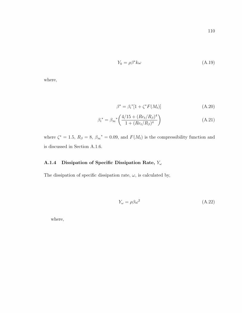
110

Yk = ρβ∗kω (A.19)

where,

β∗ = βi∗[1 + ζ∗F (Mt)] (A.20)

βi∗ = β∞

∗(

4/15 + (Ret/Rβ)4

1 + (Ret/Rβ)4

)(A.21)

where ζ∗ = 1.5, Rβ = 8, β∞∗ = 0.09, and F (Mt) is the compressibility function and

is discussed in Section A.1.6.

A.1.4 Dissipation of Specific Dissipation Rate, Yω

The dissipation of specific dissipation rate, ω, is calculated by,

Yω = ρβω2 (A.22)

where,

111

β = βi

[1− β∗i

βiζ∗F (Mt)

](A.23)

βi = Flβi,1 + (1− Fl)βi,2 (A.24)

Fl = tanh(φ4l ) (A.25)

φl = min

[max

( √k

0.09ωy,500µ

ρy2ω

),

4ρk

σω,2Dω+y2

](A.26)

Dω+ = max

[2ρ

1

σω,2

1

ω

∂k

∂xj

∂ω

∂xj, 10−10

](A.27)

A.1.5 Compressibility Function, F (Mt)

The compressibility function used in Equations A.19 and A.22 is calculated by the

following,

F (Mt) =

0 Mt ≤Mt0

Mt2 −Mt0

2 Mt > Mt0

(A.28)

where,

Mt2 ≡ 2k

a2(A.29)

Mt0 = 0.25 (A.30)

a =√γRT (A.31)

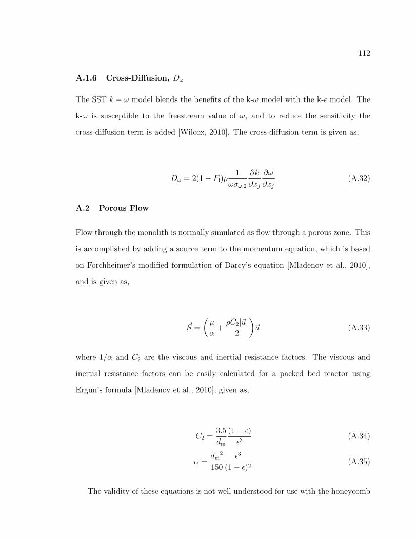
112

A.1.6 Cross-Diffusion, Dω

The SST k − ω model blends the benefits of the k-ω model with the k-ε model. The

k-ω is susceptible to the freestream value of ω, and to reduce the sensitivity the

cross-diffusion term is added [Wilcox, 2010]. The cross-diffusion term is given as,

Dω = 2(1− Fl)ρ1

ωσω,2

∂k

∂xj

∂ω

∂xj(A.32)

A.2 Porous Flow

Flow through the monolith is normally simulated as flow through a porous zone. This

is accomplished by adding a source term to the momentum equation, which is based

on Forchheimer’s modified formulation of Darcy’s equation [Mladenov et al., 2010],

and is given as,

~S =

(µ

α+ρC2|~u|

2

)~u (A.33)

where 1/α and C2 are the viscous and inertial resistance factors. The viscous and

inertial resistance factors can be easily calculated for a packed bed reactor using

Ergun’s formula [Mladenov et al., 2010], given as,

C2 =3.5

dm

(1− ε)ε3

(A.34)

α =dm

2

150

ε3

(1− ε)2(A.35)

The validity of these equations is not well understood for use with the honeycomb

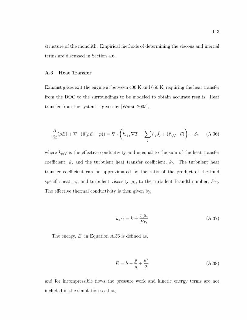
113

structure of the monolith. Empirical methods of determining the viscous and inertial

terms are discussed in Section 4.6.

A.3 Heat Transfer

Exhaust gases exit the engine at between 400 K and 650 K, requiring the heat transfer

from the DOC to the surroundings to be modeled to obtain accurate results. Heat

transfer from the system is given by [Warsi, 2005],

∂

∂t(ρE) +∇ · (~u(ρE + p)) = ∇ ·

(keff∇T −

∑j

hj ~Jj + (¯τeff · ~u)

)+ Sh (A.36)

where keff is the effective conductivity and is equal to the sum of the heat transfer

coefficient, k, and the turbulent heat transfer coefficient, kt. The turbulent heat

transfer coefficient can be approximated by the ratio of the product of the fluid

specific heat, cp, and turbulent viscosity, µt, to the turbulent Prandtl number, Prt.

The effective thermal conductivity is then given by,

keff = k +cpµtPrt

(A.37)

The energy, E, in Equation A.36 is defined as,

E = h− p

ρ+u2

2(A.38)

and for incompressible flows the pressure work and kinetic energy terms are not

included in the simulation so that,

114

E = h =∑j

Yjhj (A.39)

hj =

∫ T

Tref

cp,jdT (A.40)

where hj is the enthalpy of species j, Yj is the mole fraction of species j, cp,j is the

specific heat of species j, and Tref is the reference temperature.

115

Appendix B

Uncertainty

A description of the method used to calculate uncertainty in the experimental results.

B.1 Theory

The error is defined as the difference between the true value and the measured value

[Moffat, 1988]. Since the true value is almost never known, the uncertainty in the

experimental value is calculated using standard statistical methods, where the mea-

sured value is used as a basis for defining a range in which the actual value may fall.

The range represents the likelihood of containing the actual value with the probability

typically being called the confidence level [Moffat, 1988].

For any measurement using any measurement system, the uncertainty is a com-

bination of the bias and precision uncertainty. The bias uncertainty is the accuracy

of the measurement device or the maximum expected error introduced by the device

within a given confidence interval. the desired value and is usually small in com-

parison to the precision uncertainty where the precision uncertainty is the result of

random error components that affect the measurement of the desired value, for exam-

ple random changes in environmental conditions that result in an inability to exactly

replicate the results from one test to the next [Moffat, 1988].

The precision uncertainty represents the random error components beyond the

116

error of the measuring device. For a measured variable, Xi, the precision uncertainty,

δXi, is calculated using the following,

δXi = tSx√N

(B.1)

where t is the corresponding Student’s t-distribution statistic, Sx is the sample stan-

dard deviation, and N is the number of samples [Moffat, 1988].

The overall uncertainty is calculated as the as the root sum of squares of the bias

and precision uncertainty. In cases where the precision uncertainty is a minimum

of an order of magnitude larger than the bias uncertainty, the overall uncertainty is

taken simply as the precision uncertainty.

Using measured variables to further calculate parameters results in a need to

propagate the uncertainty through the calculations. When the calculation involves a

single measured variable, the uncertainty in the calculated variable, RXi, is calculated

by [Moffat, 1988],

δRXi=

∂R

∂Xi

δXi (B.2)

For calculations involving multiple independent measured variables, the overall

uncertainty, δR, is calculated by [Moffat, 1988],

δR =

[ N∑i=1

(∂R

∂Xi

δXi

)2] 12

(B.3)

where the contribution in uncertainty of each measured variable, δXi, contributes to

the overall uncertainty [Moffat, 1988].