Characterization of residential chimney conditions for flue

ISSN 1401 - 7555

ISRN DU-SERC- -98- -SE

Characterization of residential chimney conditions for flue gas

flow measurements

March 2012

Janne Paavilainen

ABSTRACT A literature survey and a theoretical study were performed to characterize residential chimney conditions for flue gas flow measurements. The focus is on Pitot-static probes to give sufficient basis for the development and calibration of a velocity pressure averaging probe suitable for the continuous dynamic (i.e. non steady state) measurement of the low flow velocities present in res-idential chimneys. The flow conditions do not meet the requirements set in ISO 10780 and ISO 3966 for Pitot-static probe measurements, and the methods and their uncertainties are not valid.

The flow velocities in residential chimneys from a heating boiler under normal operating condi-tions are shown to be so low that they in some conditions result in voiding the assumptions of non-viscous fluid justifying the use of the quadratic Bernoulli equation. A non-linear Reynolds number dependent calibration coefficient that is correcting for the viscous effects is needed to avoid significant measurement errors.

The wide range of flow velocity during normal boiler operation also results in the flow type chang-ing from laminar, across the laminar to turbulent transition region, to fully turbulent flow, resulting in significant changes of the velocity profile during dynamic measurements. In addition, the short duct lengths (and changes of flow direction and duct shape) used in practice are shown to result in that the measurements are done in the hydrodynamic entrance region where the flow velocity profiles most likely are neither symmetrical nor fully developed. A measurement method insensi-tive to velocity profile changes is thus needed, if the flow velocity profile cannot otherwise be de-termined or predicted with reasonable accuracy for the whole measurement range.

Because of particulate matter and condensing fluids in the flue gas it is beneficial if the probe can be constructed so that it can easily be taken out for cleaning, and equipped with a locking mechanism to always ensure the same alignment in the duct without affecting the calibration.

The literature implies that there may be a significant time lag in the measurements of low flow rates due to viscous effects in the internal impact pressure passages of Pitot probes, and the significance in the discussed application should be studied experimentally.

The measured differential pressures from Pitot-static probes in residential chimney flows are so low that the calibration and given uncertainties of commercially available pressure transducers are not adequate. The pressure transducers should be calibrated specifically for the application, preferably in combination with the probe, and the significance of all different error sources should be investigated carefully.

Care should be taken also with the temperature measurement, e.g. with averaging of several sen-sors, as significant temperature gradients may be present in flue gas ducts.

SAMMANFATTNING En litteraturstudie och en teoretisk studie gjordes för att karaktärisera omständigheterna i villa-skorstenar för mätningar av rökgasflöden. Studien har fokuserat på Pitotrör för att få tillräckligt underlag för utveckling och kalibrering av ett medeltrycksbildande mätdon lämpad för dynamiska (icke-stationära) mätningar av låga flödeshastigheter i villaskorstenar. Flödesförhållandena upp-fyller inte de krav som ges i ISO 10780 och ISO 3966 för mätningar med Pitotrör, och därmed är inte dess metoder och mätosäkerheter giltiga.

Studien visar att normala flödeshastigheter i skorstenar för villapannor är så låga att de antagan-den som görs om icke-viskösa fluider vid mätning med Pitotrör inte är giltiga. En olinjär Reynolds tal korrelerad kalibreringskoefficient behövs därför för att undvika betydliga mätfel.

De stora skillnaderna i flödeshastighet som uppstår vid normaldrift av en panna resulterar också i att flödeskaraktäristiken ändras från laminärt, via övergångsregionen till fullt utvecklat turbulent flöde, vilket orsakar betydliga förändringar i flödeshastighetsprofilen under dynamiska mätningar. Utöver detta resulterar de i praktiken korta avstånden (samt förändringarna i riktning och tvär-snitt) att mätningarna ofta görs i den hydrodynamiska inloppszonen där flödeshastighetsprofiler-na sannolikt är varken symmetriska eller fullt utvecklade. Därför finns det behov av en mätmetod som är okänslig för förändringar i flödeshastighetsprofilen, om inte profilen på annat sätt kan fastställas eller förutsägas med rimlig noggrannhet över hela mätområdet.

På grund av partiklar och eventuellt kondenserande vätskor i rökgaserna är det en fördel om mätsonden kan konstrueras så att den kan lätt tas ut för rengöring samt med låsmekanism som försäkrar samma orientering med flödet för att inte påverka kalibreringen.

Litteraturen antyder att det kan förekomma betydliga tidsfördröjningar i mätningar av låga flöden på grund av viskösa krafter i interna smala tryckledningarna i Pitot sonder, och betydelsen av dessa i diskuterade tillämpningen borde utredas experimentellt.

De uppmätta differenstrycken från Pitot-statiska mätdon i villaskorstenar är så låga att kalibre-ringen och mätosäkerheterna som anges för kommersiellt tillgängliga tryckgivare inte är tillämp-bara. Tryckgivarna bör kalibreras specifikt för tillämpningen, helst i kombination med mätdonet, och inverkan av alla av olika felkällor utredas noggrant.

Hänsyn bör också tas till temperaturförhållanden, t.ex. genom medelvärdesbildning av flera gi-vare, då stora temperaturvariationer och betydande temperaturgradienter kan förekomma i rök-gaskanaler.

TABLE OF CONTENTS Abstract ..................................................................................................................................................... Sammanfattning ....................................................................................................................................... Table of Contents ..................................................................................................................................... 1 Introduction ..................................................................................................................................... 2

1.1 Background ............................................................................................................................. 2 1.2 Purpose, Method and Scope ................................................................................................. 3

2 Known issues in flue gas flow measurement ............................................................................... 4 3 Chimney flow characteristics ......................................................................................................... 8

3.1 Residential Chimney Boundary Conditions ........................................................................... 8 3.2 Definition of the Reynolds Number ....................................................................................... 8 3.3 Average Bulk Reynolds Number and Flow Type ................................................................... 9

3.3.1 Critical Reynolds Number and Flow Type Transition .................................................... 9 3.3.2 Reynolds Numbers and Flow Types in Residential Chimneys ................................... 10 3.3.3 Intermittency and Hysteresis of Flow Type Transition ................................................ 11

3.4 Flow Velocity Profiles ............................................................................................................ 11 3.4.1 Fully Developed Velocity Profiles ................................................................................. 11 3.4.2 Hydrodynamic entrance region .................................................................................... 13 3.4.3 Single Point Velocity Measurement Methods ............................................................. 15 3.4.4 Experimental Determination of Chimney Flow Velocity Profiles ................................ 16 3.4.5 Significance of Velocity Profiles in Chimney Flow Measurements ............................ 18

3.5 Viscous effects ...................................................................................................................... 19 3.5.1 Probe External Reynolds Number ................................................................................ 19 3.5.2 Probe Impact Pressure Port Reynolds Number .......................................................... 21 3.5.3 Significance of Viscous Effects in Chimney Flow Measurements ............................. 22

3.6 Wall Proximity and Stem Blockage ...................................................................................... 22 3.7 Flue gas density .................................................................................................................... 22 3.8 Average flow temperature .................................................................................................... 23 3.9 Yaw angle .............................................................................................................................. 23 3.10 Vibrations .............................................................................................................................. 24 3.11 Turbulence ............................................................................................................................ 24 3.12 Differential Pressure Measurement .................................................................................... 24 3.13 Other considerations ............................................................................................................ 24

4 Discussion and Conclusions ........................................................................................................ 26 5 Acknowledgments ........................................................................................................................ 28 6 Nomenclature ............................................................................................................................... 30 7 References .................................................................................................................................... 32

1

2

1 INTRODUCTION 1.1 BACKGROUND

With the booming conversion from direct electrical and fossil fuel to bioenergy based heating sys-tems there has been increasing interest in determining the efficiency, and characterizing and quantifying the emissions (e.g. carbon monoxide, hydrocarbons, nitric oxides, particles) of resi-dential heating boilers (single- to multi-family house size), e.g. [1-3]. Arguments and evidence have been presented that the steady state testing methods of boilers, such as EN-303 [4], do not represent the normal intermittent and transient operation (start, stop and combustion power modulation) of such boilers in real applications, e.g. [5-7]. Especially in the case of solid fuel boil-ers work has been done to develop methods for quantifying the efficiency and emissions on a yearly basis with a combination of transient simulations and boiler models validated by laboratory measurements [5, 8-11], with the further purpose of finding solutions to improve the systems. For quantifying the emissions under dynamic conditions a continuous measurement of the flue gas flow rate is needed.

For determining the combustion (and flue gas flow) rate a scale is normally used for measuring the solid fuel consumption of a burner, but the amounts of fuel combusted during short transients are usually too small compared to the scale resolution and measurement errors to deduce useful data with reasonable uncertainty [8, 9]. The combustion rate can also be determined indirectly from the flue gas flow rate combined with a flue gas analysis when the fuel composition is known [5, 10, 12]. Such a method can also be used in field measurement studies where the use of a scale would be practically impossible. For both research and benchmark testing purposes it is thus beneficial to be able to do reliable continuous (i.e. logging data over longer periods) dynamic (i.e. non steady state) measurements of flue gas flow rates from single family house size heating boilers. However, the flow conditions in ducts and chimneys during normal boiler operation of these boilers are challenging from a measurement engineering point of view:

The low flow velocities and geometrical conditions (flow disturbances) in the chimneys normally do not meet the requirements for Pitot-static tube measurements according to ISO 10780 and ISO 3966. However, the standards do not readily provide methods for tak-ing into account the various measurement error sources under these conditions.

Methods causing higher pressure drops to the flow than the Pitot-static method would be significantly more accurate, but prevent realistic operation of the burner, and cannot be used outside of laboratory environment.

Clogging due to particulate deposits and condensation causes easily measurement errors and thus the probe should be easy to clean frequently without disturbing the operation of the boiler and preserving the calibration of the probe.

3

1.2 PURPOSE, METHOD AND SCOPE

The purpose of this work is to characterize the chimney flow conditions of residential boilers for choosing and improving measurement methods. The focus is on issues with Pitot (-static) type probes as these are well studied, standardized and widely used, inducing a relatively low perma-nent pressure drop to the flow, and can be constructed easy to maintain. Averaging multi-port Pitot probes can also take into account non-symmetric and changing velocity profiles. Some of the results may be interesting also regarding other flow measurement methods, mainly those produc-ing a differential pressure.

A literature survey is done to find out the results of previous work and current state of art mainly regarding Pitot-static measurements of fluid flows. The area is widely researched and there is an extensive literature resource available. Thus to keep the reference list manageable, mostly gen-eral summary type references are preferred, and specialized sources regarding the discussed topic are referred to where suitable.

Based on the literature survey a theoretical study is done where the main purpose is to character-ize the flow conditions in the specific case residential chimneys. The results are presented and compared with literature in a manner that gives a general view to cover the wide operating ranges of various types of residential solid fuel boilers for the purpose of evaluating the impact of pre-dictable physical effects on flue gas flow rate measurements. This is needed both for justifying the choice of a measurement method and helping in interpreting calibration results, and possibly leading to improved correlations and measurement uncertainty.

Some velocity profile measurements are also performed and the results analyzed to confirm some of the theoretical phenomena in effect.

4

2 KNOWN ISSUES IN FLUE GAS FLOW MEASUREMENT For continuous dynamic flue gas flow measurements a single point velocity pressure measure-ment with a standard L-type (or S-type) Pitot-static tube is often done, assuming a certain velocity profile based on initial traversing measurements [13, 14]. This method is practically difficult to calibrate for the whole range of boiler operation as it would require long enough steady states at different combustion rates for the traversing measurements to be successful. Arbitrary steady states of sufficient durations are often prevented by both boiler system control algorithms and limitations of the heating load (which especially in field conditions often is the only available heat dump).

Several of the assumptions (or requirements) regarding the use of the Pitot-static method in chimney flue gas flows also become potentially invalid in some operational states of boilers, es-pecially at low combustion powers. Robinson [15] summarizes the requirements set in ISO 10780 [13], which are met questionably (or not met at all) in industrial stack flows, arguing that a simple calibration coefficient is probably not sufficient to cover the wide range of operating conditions. The significance the different error sources in stack flows should be considered and the deter-mined calibration coefficients cannot be used in other conditions or generalized based on e.g. similar geometry without reconsidering the new setting [16-18].

Calibration coefficient dependency on the Reynolds number

The calibration coefficients of Pitot(-static) tubes are non-linear with low Reynolds numbers ( ). Based on theory there is a predictable change in flow meter response at low because viscous effects become gradually significant the lower the flow velocity and therefore the normally used quadratic Bernoulli correlation, which assumes non-viscous fluids, becomes gradually invalid when the is below a certain level [18-22]. ISO 10780 [13] sets 1200 (Pitot tube local conditions) as a requirement stating that below this limit the Pitot tubes are a subject to signif-icant errors, and a requirement of 200 based on the impact pressure hole diameter of the Pitot tube is set in ISO 3966 [14]. These requirements may not be met with standard Pitot tubes in typical residential chimney flow velocities. Thus a calibration of the probe in the final environment is needed for the determination of the probe calibration factor as a function of for the expected operating range.

ISO 10780 [13] states that outside the 5 to 50m/s flow velocity range (Pitot tube local condi-tions) the probe must be specifically calibrated for the intended range, while Ower [18] discusses the difficulties of measuring at relatively low flow velocities and advises to switch to other meth-ods than the Pitot tube below 5m/s velocities. Flue gas flows in typical residential chimney diame-ters are almost always below 5m/s average bulk velocity.

Velocity profiles and changing flow type

Sufficient hydrodynamic entrance lengths before the flow measurement point to always justify the assumption of a fully developed velocity profile would require duct lengths that are practically difficult to achieve even in normal laboratory conditions, and are impossible in field conditions. The entrance region length is also a function of when the flow is laminar, meaning that at a fixed measurement point in the entrance region the impact of a velocity profile change can be expected to vary from insignificant to significant depending on flow conditions [23-25]. ISO 3966 emphasizes the risk of velocity profiles changing when the flow rate varies over a wide range of

5

so that a single measured flow velocity profile cannot be predicted to be valid for a wide oper-ational range of a boiler.

With relatively low flow velocities in stack conditions the same differential pressure can be achieved with different velocities, depending on duct diameter and temperature [17]. Especially under flow conditions close to critical (in the flow type transition region) the flow characteristic may vary, seemingly arbitrarily, between laminar and turbulent because of intermittent character (instability of flow type) or a hysteresis effect (flow type change happens differently dependent on whether flow rate increases or decreases), as summarized in [18, 26, 27], causing poor repeata-bility of flow meters in these conditions [21].

Differential pressure measurement

A further complication regarding differential pressure measurement methods at low flow veloci-ties is the accuracy of the pressure measurement and the issue is also briefly mentioned in [15]. The differential pressures produced by Pitot-static tubes are in the order of a few Pa while com-mercially available “low” differential pressure transducers are normally calibrated to a range of up to at least tens of Pa, resulting in that they are used at, and way below, the lowest 10% of their intended measurement range when using for chimney flow measurements. Issues such as meas-urement uncertainty, resolution and environmental error sources thus may become significant problems and should be evaluated.

Reported practical experiences

The Swedish Institute of Applied Environmental Research (ITM) does testing of accredited emis-sions monitoring organizations. ITM has reported the results of tests where a number of organiza-tions in field measurement conditions independently measured a stack flow from a boiler with their preferred Pitot-static method (S or L probe) [28, 29]. The measurements are compared to a reference method and the comparison shows that even when meeting the flow velocity require-ments set in ISO 10780 [13] the results of the independent measurements varied ±15% from the reference flow rate. A similar test was done also in laboratory conditions at different flow veloci-ties [30]. The results imply that even in controlled laboratory conditions, where all ISO 10780 requirements are met, one can expect ±10% deviations. The UK National Physical Laboratory performed a questionnaire survey to the UK emissions monitoring community [15] with the re-sults that a significant number of organizations were routinely performing measurements outside of the conditions given in ISO 10780, although the reference does not summarize how the organ-izations dealt with this. No standardized or recommended methods for correcting the measure-ment or estimating the uncertainty outside the ISO 10780 requirements are readily provided by the standard.

Need for development of methods for residential chimney conditions

As a conclusion based on the above presented issues it can be said, that even though differential pressure based flow measurement methods, and especially the Pitot (-static) method, are a wide-ly used and proven technique, in stack flow conditions there is potential for relatively large meas-urement errors, which should either be calibrated for, or properly taken into account in the uncer-tainty analysis. Based on theory and earlier work there is a potentially significant non-linear change in the response of differential pressure based measurement equipment in the relatively low chimney flue gas flow velocities due to viscous effects, and the situation is aggravated be-

6

cause of the uncertainty and potential errors of the differential pressure measurement. The re-sults of the survey on the UK measuring community seem to imply that it is difficult to strictly ap-ply the standard methods already for industrial scale boilers, and the Swedish comparisons of independent Pitot-static measurements done by professionals in ideal measurement conditions imply uncertainties and repeatability which may not be satisfactory for benchmark testing and research purposes, based on which one could expect similar problems likely also for smaller boil-ers. For residential boiler chimneys the flow conditions are probably always completely outside of the ISO 10780 [13] requirements, so the method and its stated uncertainties cannot be applied as such without an analysis of the conditions.

As there is a growing need to cost-effectively do continuous dynamic flue gas measurements in residential boiler chimneys for both research and benchmark testing purposes, there is also a need to improve the measurement methods for the purpose, and to gain knowledge about the uncertainties.

Although this literature study is regarding mostly the Pitot(-static) method, it should be noted that many other in-flow probing flow measurement methods also suffer, at least partly, from the same physical effects at low flow rates, due to viscous effects at low . Based on the literature availa-ble, many of the low physical phenomena are already studied in detail and explained, so at least some of the shortcomings of the flue gas flow measurement methods should be possible to improve if their low response in practice and uncertainties are studied, and repeatability can be shown for the intended operating range.

7

8

3 CHIMNEY FLOW CHARACTERISTICS

3.1 RESIDENTIAL CHIMNEY BOUNDARY CONDITIONS

The theoretical of flue gas flows in chimneys vary mostly dependent on fuel composition, combustion power and burner excess air setting (the three defining combined the flue gas flow rate), chimney or stack diameter, and the temperature of the flue gas entering the chimney.

The used fuel is normally wood (logs, chips, pellets), oil or gas. Other fuels are also used, e.g. the use of field crops pressed to pellets is becoming more popular. Flue gas from wood combustion is assumed throughout this study, although the properties of the other flue gases from other fuels mentioned are close enough for the conclusions to be generalized in most cases.

The kinematic viscosity of 50 to 200ºC flue gas (from biomass combustion) is about 10 to 15% lower compared to air, and since it is the divider in Eq. 1 the effect is similar also on , inversely, so that the in this temperature range are 10 to 15% higher compared to air. While this does not have direct effect on volume flow rate calculation it may have a small impact on evaluating the flow characteristics (e.g. turbulent or laminar). The calculated in the following sections are based on typical wood combustion flue gas viscosity, not air.

Typical residential chimney internal diameters vary approximately from 80 to 100 (although larger diameters are not uncommon). These two values are used as example throughout the study and will be referred to as D80 and D100.

Typical single family house residential boiler nominal thermal power outputs vary from approxi-mately 10 to 20kW with thermal efficiencies ranging from 0.7 to over 0.9, modern typical boilers having about 0.90.

Operating ranges of the burners vary from 0% at startup to a normal combustion power modula-tion operation between 30% and 100% of nominal.

Combustion excess air ratios vary also greatly, especially between different fuels and combustion techniques. With oil and gas burners air ratios less than 1.3 may be used, whereas for pellet boil-ers they may range from 1.5 to 2.5 or more within the operating range.

Flue gas temperatures can vary from room temperature at startup up to 200ºC (or more) during nominal combustion power.

The absolute pressure levels in residential chimneys are normally between 5 to 20Pa below the ambient pressure, i.e. small enough variation to have negligible effects on fluid properties.

3.2 DEFINITION OF THE REYNOLDS NUMBER

Flow characteristics relevant to flow measurement are usually related to the dimensionless Reyn-olds number ( ).

9

Eq. 1.

It should be noted that when discussing flow characteristics and flow measurements the can be defined in different ways. Usually, when talking about internal flows in e.g. ducts, is based on the average bulk flow velocity in the duct and the internal hydraulic diameter of the duct. When talking about an in-flow probe, e.g. a Pitot-static tube, is usually based on its (outer) hydraulic radius and the local flow velocity. A third definition is based on the probe impact pressure port radius to check for possible viscous damping effects in the internal tube passage. Other charac-teristic measures are also used for the probe, e.g. probe diameters or lengths instead of radii. These definitions can easily cause confusion as the definition depends on the subject discussed, which can change even within the same sentence. Also adding to the confusion is mixing the use of radii with the engineering praxis of using diameters when e.g. pipe and bore hole dimensions are discussed. Therefore, unless otherwise mentioned, the following subscripts will be used to differentiate the probe related external and internal from the bulk flow :

BAV – Bulk Average Velocity (i.e. ), and it is based on the duct internal hydrau-lic diameter and average bulk flow velocity.

POR – Probe Outer Radius (i.e. ), and is be based on the outer probe radius and local flow velocity.

PIR – Probe Internal Radius (i.e. ), and it is based on the impact pressure port radius and local flow velocity.

3.3 AVERAGE BULK REYNOLDS NUMBER AND FLOW TYPE

3.3.1 CRITICAL REYNOLDS NUMBER AND FLOW TYPE TRANSITION

Starting with a laminar flow type, gradually increasing the flow rate the flow becomes unstable (labile) when the is greater than the critical Reynolds number . An experimentally shown and generally accepted limit is 2300, although a value of 2000 is also sometimes used, e.g. [18, 23, 26, 27]. is actually not a fixed value, and depends on the upstream flow conditions, inlet configuration, pipe internal surface roughness, and whether the flow rate is increasing or decreasing [26, 27]. While it is reported that under special conditions laminar flows can occur far beyond 2300, there is a somewhat stricter lower limit of

2000, below which the flow can be said almost always to be laminar even with strong disturbances in the flow, because of predominant viscous forces quickly damping any disturb-ances [26, 27]. When it indicates that even a small disturbance can change the flow from laminar to turbulent and thus a similar more fixed limit as the 2000 cannot be generalized for when the flow always could be said to be turbulent, as it is dependent on the vari-ous factors mentioned. Different values can be found in literature, ranging 3000 ≲ ≲10000, [22, 23, 25, 26], although these are usually laboratory results for smooth pipes with care-ful initial conditioning, and for most practical engineering applications 2000 ≲ ≲ 4000 can be assumed [26]. This range, where the transition from laminar to turbulent flow is most likely to happen, is generally referred to as the transition region (or e.g. transition zone, critical region) and should not be confused as a region of gradual transition of a specific fluid flow (although a gradu-al transition may occur in the hydrodynamic entrance region as explained later).

10

3.3.2 REYNOLDS NUMBERS AND FLOW TYPES IN RESIDENTIAL CHIMNEYS

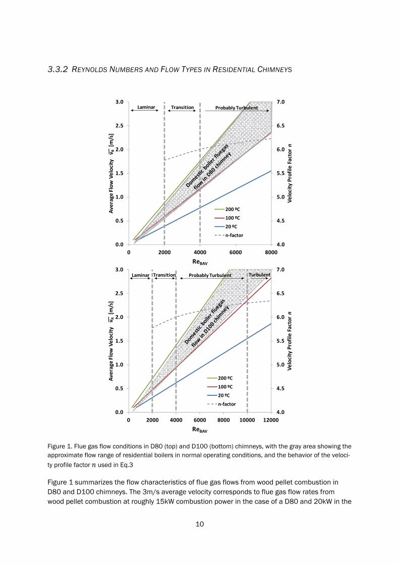
Figure 1. Flue gas flow conditions in D80 (top) and D100 (bottom) chimneys, with the gray area showing the approximate flow range of residential boilers in normal operating conditions, and the behavior of the veloci-

ty profile factor used in Eq.3

Figure 1 summarizes the flow characteristics of flue gas flows from wood pellet combustion in D80 and D100 chimneys. The 3m/s average velocity corresponds to flue gas flow rates from wood pellet combustion at roughly 15kW combustion power in the case of a D80 and 20kW in the

4.0

4.5

5.0

5.5

6.0

6.5

7.0

0.0

0.5

1.0

1.5

2.0

2.5

3.0

0 2000 4000 6000 8000

Velocity Profile Factor n

Average

Flow Velocity vR[m

/s]

ReBAV

200 ºC

100 ºC

20 ºC

n‐factor

Probably TurbulentLaminar Transition

4.0

4.5

5.0

5.5

6.0

6.5

7.0

0.0

0.5

1.0

1.5

2.0

2.5

3.0

0 2000 4000 6000 8000 10000 12000

Velocity Profile Factor n

Average

Flow Velocity vR[m

/s]

ReBAV

200 ºC

100 ºC

20 ºC

n‐factor

TransitionLaminar TurbulentProbably Turbulent

11

case of a D100 chimney, with the fuel moisture content being around 7% wet basis, excess air ratio of 2.

The gray area shows approximately the flow range when the combustion power is modulated from startup (which can be close to zero air leakage flow rate at room temperature) to full nominal combustion power (flue gas at around 100-200ºC). Boilers and burners of different types end up in various operational states depending on the combustion technique, fuel properties and burner settings, and thus the gray area also covers a wide range of temperatures and excess air ratios. The calculated average flow velocities are consistently below the 5 to 50m/s validity range given in ISO 10780 [13].

The values 2000, 4000 and 10000 are also shown for giving an esti-mation of the flow characteristic, keeping in mind that for 4000 the flow type is most likely turbulent in chimney conditions. It can be seen that the normal flue gas flow characteristics for these boilers range from laminar, over the transition region, reaching into a region where one can be relatively certain of a fully developed turbulent flow, meaning that dynamic measurement methods need to take into account all these characteristics.

3.3.3 INTERMITTENCY AND HYSTERESIS OF FLOW TYPE TRANSITION

Near the limit an intermittent state of flow type, where sequential changes from laminar to turbulent and back are happening, has been studied experimentally and correction factors are suggested, [26, 27]. This kind of intermittency is more likely to happen in long and narrow pipes [26] and thus probably not a concern in the relatively short and wide residential chimneys. It is also unlikely that long lived steady states would frequently occur near in residential chim-neys.

A transition hysteresis has also been experimentally confirmed, meaning that is different for increasing and decreasing in the same flow. The transition from laminar to turbulent has a higher than in the opposite transition [26]. The transition causes a change in velocity profile as described in section 3.4. The flue gas flows from some boilers may be frequently cross-ing the transition region and whether the hysteresis has impact on dynamic flue gas flow meas-urements should be experimentally investigated.

3.4 FLOW VELOCITY PROFILES

3.4.1 FULLY DEVELOPED VELOCITY PROFILES

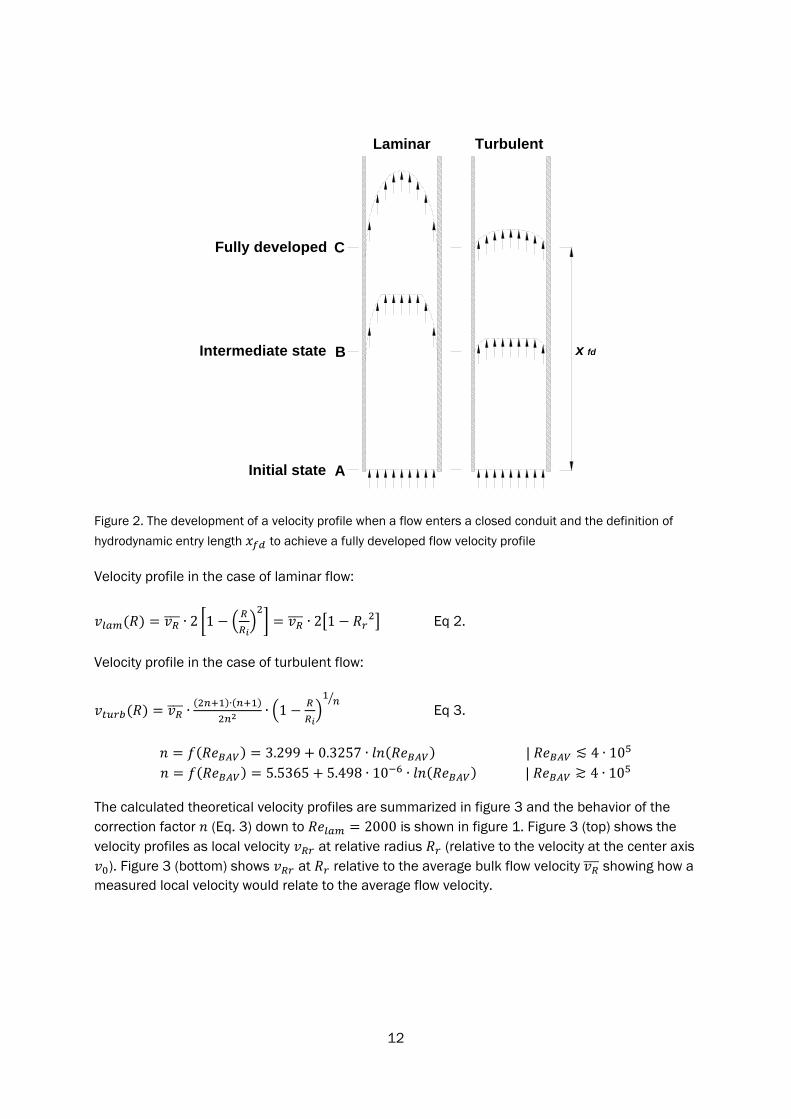
In closed conduits viscous forces cause a flow velocity profile to form such that the fluid flows slower close to the walls. Both theory and experiments have shown that a change in the flow type from laminar to turbulent causes a change in the velocity profile, e.g. [18, 21, 26, 27]. The fully developed velocity profile is assumed always parabolic when the flow is laminar, but with turbu-lent flow it is a function of . These profiles are shown in figure 2, case C (fully developed). Eq.2 and eq.3 for calculating the velocity profiles are found in [22, 27]. For the turbulent flow also variants dependent on pipe surface roughness can be found in literature, e.g. [23], of which eq. 3 is a simplification for engineering applications with typical pipe surface roughness (i.e. pipe factor does not change significantly).

12

Figure 2. The development of a velocity profile when a flow enters a closed conduit and the definition of

hydrodynamic entry length to achieve a fully developed flow velocity profile

Velocity profile in the case of laminar flow:

∙ 2 1 ∙ 2 1 Eq 2.

Velocity profile in the case of turbulent flow:

∙∙

∙ 1 Eq 3.

3.299 0.3257 ∙ | ≲ 4 ∙ 105.5365 5.498 ∙ 10 ∙ | ≳ 4 ∙ 10

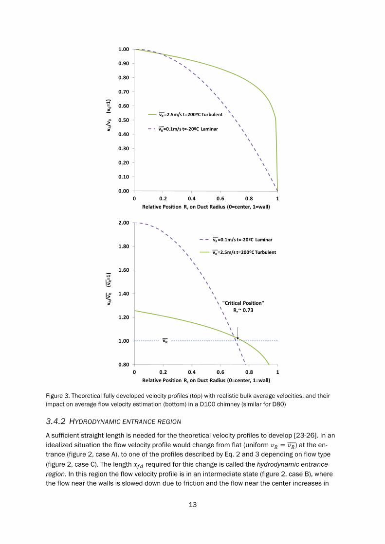
The calculated theoretical velocity profiles are summarized in figure 3 and the behavior of the correction factor (Eq. 3) down to 2000 is shown in figure 1. Figure 3 (top) shows the velocity profiles as local velocity at relative radius (relative to the velocity at the center axis

). Figure 3 (bottom) shows at relative to the average bulk flow velocity showing how a measured local velocity would relate to the average flow velocity.

x fd

TurbulentLaminar

Fully developed

Initial state

Intermediate state

A

B

C

13

Figure 3. Theoretical fully developed velocity profiles (top) with realistic bulk average velocities, and their impact on average flow velocity estimation (bottom) in a D100 chimney (similar for D80)

3.4.2 HYDRODYNAMIC ENTRANCE REGION

A sufficient straight length is needed for the theoretical velocity profiles to develop [23-26]. In an idealized situation the flow velocity profile would change from flat (uniform ) at the en-trance (figure 2, case A), to one of the profiles described by Eq. 2 and 3 depending on flow type (figure 2, case C). The length required for this change is called the hydrodynamic entrance region. In this region the flow velocity profile is in an intermediate state (figure 2, case B), where the flow near the walls is slowed down due to friction and the flow near the center increases in

0.00

0.10

0.20

0.30

0.40

0.50

0.60

0.70

0.80

0.90

1.00

0 0.2 0.4 0.6 0.8 1

v R/v

0 (v

0=1)

Relative Position Rr on Duct Radius (0=center, 1=wall)

vR =0.1m/s t=‐20ºC Laminar

vR =2.5m/s t=200ºC Turbulent

0.80

1.00

1.20

1.40

1.60

1.80

2.00

0 0.2 0.4 0.6 0.8 1

v R/v

R (v

R=1)

Relative Position Rr on Duct Radius (0=center, 1=wall)

"Critical Position"Rr ~ 0.73

vR

vR =0.1m/s t=‐20ºC Laminar

vR =2.5m/s t=200ºC Turbulent

14

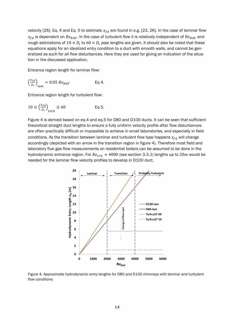
velocity [26]. Eq. 4 and Eq. 5 to estimate are found in e.g. [23, 26]. In the case of laminar flow

is dependent on . In the case of turbulent flow it is relatively independent of and rough estimations of 10 to 60 pipe lengths are given. It should also be noted that these equations apply for an idealized entry condition to a duct with smooth walls, and cannot be gen-eralized as such for all flow disturbances. Here they are used for giving an indication of the situa-tion in the discussed application.

Entrance region length for laminar flow:

0.05 Eq 4.

Entrance region length for turbulent flow:

10 ≲ ≲ 60 Eq 5.

Figure 4 is derived based on eq.4 and eq.5 for D80 and D100 ducts. It can be seen that sufficient theoretical straight duct lengths to ensure a fully uniform velocity profile after flow disturbances are often practically difficult or impossible to achieve in small laboratories, and especially in field conditions. As the transition between laminar and turbulent flow type happens will change accordingly (depicted with an arrow in the transition region in figure 4). Therefore most field and laboratory flue gas flow measurements on residential boilers can be assumed to be done in the hydrodynamic entrance region. For 4000 (see section 3.3.1) lengths up to 20 would be needed for the laminar flow velocity profiles to develop in D100 duct.

Figure 4. Approximate hydrodynamic entry lengths for D80 and D100 chimneys with laminar and turbulent flow conditions

0

2

4

6

8

10

12

14

16

18

20

0 1000 2000 3000 4000 5000 6000

Hydrodynam

ic Entry Length x

fd[m

]

ReBAV

D100‐lam

D80‐lam

Turb x/d~60

Turb x/d~10

Laminar Transition Probably Turbulent

Chan

ge of flow type

15

For comparison, ISO 3966 suggests a straight conduit with the length of 20 upstream and 5 downstream (total 25 ) for round circular cross sections in order for the flow to be “substantially parallel and symmetrical about the conduit axis”. ISO 10780 requirements state 5 of straight duct upstream and downstream (total 10 ).

In laminar cases is strongly dependent on and the transition between laminar and tur-

bulent will cause a sudden change in . It thus can be expected that at a fixed measurement point within the hydrodynamic entrance region the velocity profile will change significantly de-pendent on the . I.e. within the a traversing measurement is always required to deter-mine the new velocity profile if the flow rate or temperature (i.e. viscosity and thus ) chang-es.

In the intermediate state (see figure 2) in the entrance region the flow may also be laminar in the periphery and turbulent in the core of the cross section, i.e. a semi-turbulent state which can exist over a wide range of . In the semi-turbulent state changes in only alter the relative size of the turbulent core and with decreasing the laminar periphery grows thicker and the turbulent core gradually disappears without abrupt changes [26].

Changes in the duct geometry (e.g. diameter, bend, cross section) can cause asymmetric (skewed, distorted) velocity profiles downstream. Even though Eq.4. and Eq.5 are valid for an idealized entry situation with smooth duct walls, the physical principles governing the formation of the velocity profile are also valid for other disturbances, so that e.g. skewed velocity profiles caused by bends will change in a similar manner, also needing a as discussed in e.g. [21, 24]. In special cases, such as two subsequent 90º bends in different planes may cause rotation in the flow that will affect the velocity profile a relatively long distance downstream.

3.4.3 SINGLE POINT VELOCITY MEASUREMENT METHODS

The standards ISO 3966 and ISO 10780 use a traversing sampling method to take into account the actual flow velocity profile. There are also methods for determining the flow rate in a round duct with a single point measurement.

Theoretical velocity profile method

A method for measuring the flow rate with a single center (or arbitrary) point measurement would be to use the pipe factor, as described in [20]. The method is based on that the velocity profile in fully developed flows is a function of pipe surface roughness and and can thus be predict-ed with the help of the Moody’s diagram. Eq.2 and Eq.3 in section 3.4.1 are a simplification of this method. The method is limited to fully developed velocity profiles and the flow type must be known.

As an extreme example, if a single point measurement is done at the center of the duct (see Fig-ure 3, bottom), it is of most importance to be certain if the velocity is either turbulent or laminar, otherwise a significant over- or under estimation by a factor of 2.00/1.25 1.6 is possible.

16

The center point measurement is recommended for duct diameters relatively small compared to the probe, where positioning the probe closer to the wall (e.g. at the critical point as described next) would result in undesirable effects due to wall proximity [18], but the method is usable if there is no change in flow characteristic or if both the change and velocity profiles are always predictable.

Critical point method

There is a method for partially taking into account the change in velocity profile using a single measurement point on the radius where the impact of the profile change is at minimum. A hori-zontal dashed line is drawn in the bottom figure 3 at 1⁄ representing the average bulk velocity. For either the turbulent or laminar case, where 1⁄ (i.e. where curve crosses the horizontal dashed line) gives for each case the where a corresponding to the can be measured. This is called the critical position, e.g. [18, 22]. In this particular case of a D100 duct, the critical position for the laminar flow is at 0.71 and for turbulent at 0.75. A critical position for measuring the average bulk velocity taking into account both laminar and tur-bulent velocity profiles with minimal error would be 0.73, where theoretically the measure-ment would underestimate laminar by 5% and overestimate turbulent by 3%, approximate-ly.

However, this theoretical critical point approach is valid only for fully developed (axisymmetric) velocity profiles and would not be of practical help in cases of skewed velocity profiles (for which skewness may also be changing as a function of ), or in the hydrodynamic entrance region (explained in next section). The critical point could still be used as aid in simplifying in situ calibra-tion of single point measurements even with asymmetric velocity profiles, in order to get a more linear response.

3.4.4 EXPERIMENTAL DETERMINATION OF CHIMNEY FLOW VELOCITY PROFILES

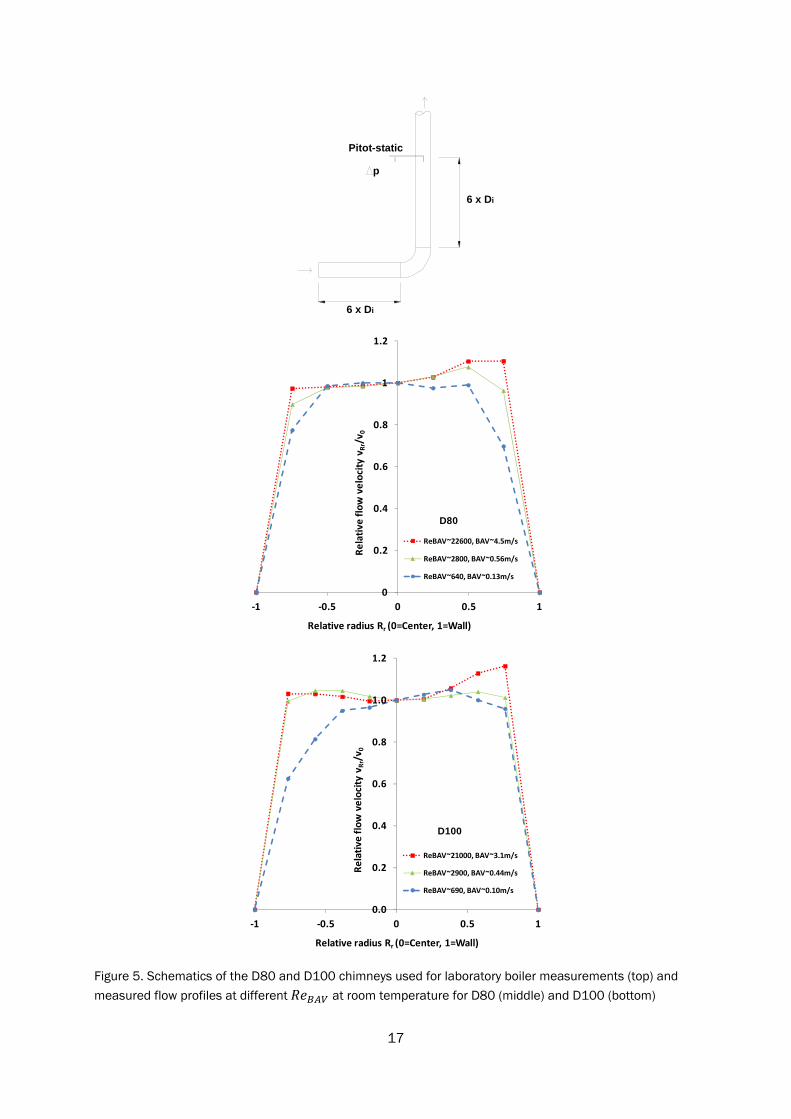
An experiment was done to determine the velocity profiles in D80 and D100 chimneys construct-ed for laboratory measurements for residential boiler testing at Dalarna University (Borlänge, Sweden). The chimney height is limited because of the laboratory room height and thus sufficient straight entrance lengths according to figure 4 cannot be reached indoors. The chimney construc-tions are shown in figure 5 (top) and the measured velocity profiles in figure 5 (middle and bot-tom). Air at room temperature was used and the velocity profile measurement was made by trav-ersing a Pitot-static ( 4 L-type) tube through seven (D80) and ten (D100) points on one diameter of the duct cross section, each point an average of 3 minutes of steady state flow sam-pled with a 10 second sampling interval. A stand with a rail was built for the probe to ensure min-imal differences in probe alignment with the flow between the traverses. The reference flow rate was measured with a set of calibrated orifice plates. The measurement was done at several

, but for clarity only the two extremes and an intermediate are shown in figure 5.

17

Figure 5. Schematics of the D80 and D100 chimneys used for laboratory boiler measurements (top) and

measured flow profiles at different at room temperature for D80 (middle) and D100 (bottom)

Pitot-static

6 x Di

p

6 x Di

0

0.2

0.4

0.6

0.8

1

1.2

‐1 ‐0.5 0 0.5 1

Relative

flow velocity v

Rr/v 0

Relative radius Rr (0=Center, 1=Wall)

ReBAV~22600, BAV~4.5m/s



D80

0.0

0.2

0.4

0.6

0.8

1.0

1.2

‐1 ‐0.5 0 0.5 1

Relative

flow velocity v

Rr/v 0

Relative radius Rr (0=Center, 1=Wall)




D100

18

The observed velocity profile change was gradual and consistent with literature [26]. Comparing the measured velocity profiles to figures 2 and 3 it can be seen that in both chimneys the velocity profile changes from a turbulent type towards a laminar (parabolic) one, due to flow type change. It can also be seen that the velocity profile is skewed when turbulent, approaching symmetric when laminar, but does not reach a fully parabolic state with laminar flow, due to insufficient en-trance length. All of the above discussed theoretical velocity profile effects are thus shown to be in effect in the measurement, and should therefore be taken into account in chimney flue flow rate measurements. As an example, in the measured cases of figure 5, in a center point continu-ous dynamic measurement assuming for the whole range a turbulent velocity profile based on initial traversing would cause approximately 11% overestimation of laminar flows in both chim-neys.

3.4.5 SIGNIFICANCE OF VELOCITY PROFILES IN CHIMNEY FLOW MEASUREMENTS

Sections 3.4.1-3.4.4 and the presented reasoning confirmed with the experimental result imply that performing a single point continuous dynamic velocity pressure measurement in normal resi-dential boiler chimney conditions, especially at 4000, there is risk for significant errors in determining the flow rate because:

The flow velocity profile will be changing as a function of . The flow type cannot be determined continuously by the measurement itself. The flow type cannot otherwise be easily predicted with reasonable uncertainty.

(For comparison, 4000 corresponds roughly to chimney flow rates resulting from burner operation at and below 50% of nominal combustion power in the cases of D80 for 15kW and D100 for 20kW combustion power.)

The results are also implying that there is a bias for over estimation of the flow rate: Because of practical reasons the initial steady state traversing measurements for checking the velocity profile often have to be done at relatively high combustion power. The velocity profile then changes al-ways towards a parabolic one with decreasing combustion power, causing an overestimation.

A further problem is that the flow rate deduced from a velocity pressure measurement will also behave in a realistic manner in correlation to the changes in flow rate, so that there is little ap-parent warning sign of whether the measurement is flawed or not.

The upstream flow conditions will also change dependent on the boiler and burner so that a cali-bration of the chimney cannot be generalized for all boilers and connecting ducts. Thus it is of most importance to use a method that is either insensitive to, or takes continuously into account the flow velocity profile in the chimney.

One way to get better accuracy in the presence of skewed or undeveloped velocity profiles would be the use of flow conditioners upstream of the flow meter [22]. These will cause an additional pressure drop and provide a place for deposits to easily accumulate, which are both unwanted characteristics regarding residential chimneys. Regarding a higher pressure drop it would make more sense to improve the accuracy by increasing the pressure drop caused by the probe (thus providing a higher differential pressure). Accumulated deposits on the flow conditioner will also probably change flow pattern affecting the calibration of the flow meter downstream.

19

3.5 VISCOUS EFFECTS

3.5.1 PROBE EXTERNAL REYNOLDS NUMBER

With low the assumption of a non-viscous fluid that the normally used Bernoulli equation re-quires becomes gradually invalid. ISO 10780 [13] gives the restriction of 1200 for the validity of its measurement uncertainties, specifically stating that below this value Pitot tubes are subject to significant errors. (It is actually not explicitly stated in the standard whether the given

is referenced to the probe diameter or the radius, although the given literature reference implies the latter is more likely. At and this limit for the viscous effects start becoming sig-nificant (sometimes also called the Barker effect).

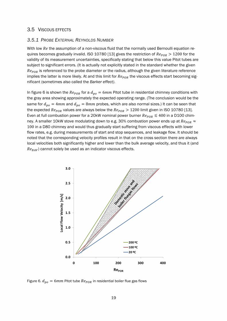
In figure 6 is shown the for a 6 Pitot tube in residential chimney conditions with the gray area showing approximately the expected operating range. (The conclusion would be the same for 4 and 8 probes, which are also normal sizes.) It can be seen that the expected values are always below the 1200 limit given in ISO 10780 [13]. Even at full combustion power for a 20kW nominal power burner ≲ 400 in a D100 chim-ney. A smaller 10kW stove modulating down to e.g. 30% combustion power ends up at 100 in a D80 chimney and would thus gradually start suffering from viscous effects with lower flow rates, e.g. during measurements of start and stop sequences, and leakage flow. It should be noted that the corresponding velocity profiles result in that on the cross section there are always local velocities both significantly higher and lower than the bulk average velocity, and thus it (and

) cannot solely be used as an indicator viscous effects.

Figure 6. 6 Pitot tube in residential boiler flue gas flows

0.0

0.5

1.0

1.5

2.0

2.5

3.0

0 100 200 300 400

Local Flow Velocity [m/s]

RePOR

200 ºC

100 ºC

20 ºC

20

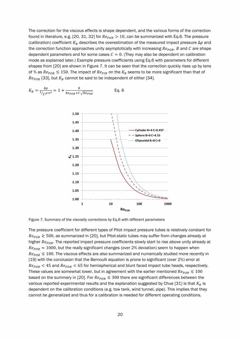
The correction for the viscous effects is shape dependent, and the various forms of the correction found in literature, e.g, [20, 31, 32] for 10, can be summarized with Eq.6. The pressure (calibration) coefficient describes the overestimation of the measured impact pressure Δ and the correction function approaches unity asymptotically with increasing . and are shape dependent parameters and for some cases 0. (They may also be dependent on calibration mode as explained later.) Example pressure coefficients using Eq.6 with parameters for different shapes from [20] are shown in Figure 7. It can be seen that the correction quickly rises up by tens of % as ≲ 150. The impact of on the seems to be more significant than that of

[33], but cannot be said to be independent of either [34].

∙ ∙1

∙ Eq. 6

Figure 7. Summary of the viscosity corrections by Eq.6 with different parameters

The pressure coefficient for different types of Pitot impact pressure tubes is relatively constant for ≳ 500, as summarized in [20], but Pitot-static tubes may suffer from changes already at

higher . The reported impact pressure coefficients slowly start to rise above unity already at 1000, but the really significant changes (over 2% deviation) seem to happen when

≲ 100. The viscous effects are also summarized and numerically studied more recently in [19] with the conclusion that the Bernoulli equation is prone to significant (over 2%) error at

45 and 65 for hemispherical and blunt faced impact tube heads, respectively. These values are somewhat lower, but in agreement with the earlier mentioned ≲ 100 based on the summary in [20]. For ≲ 300 there are significant differences between the various reported experimental results and the explanation suggested by Chue [31] is that is dependent on the calibration conditions (e.g. tow tank, wind tunnel, pipe). This implies that they cannot be generalized and thus for a calibration is needed for different operating conditions.

1.00

1.05

1.10

1.15

1.20

1.25

1.30

1.35

1.40

1.45

1.50

1 10 100 1000

KB

RePOR

Cylinder B=4 C=0.457

Sphere B=6 C=4.55

Ellipsoidal B=8 C=0

21

3.5.2 PROBE IMPACT PRESSURE PORT REYNOLDS NUMBER

There is also a requirement 100 set in ISO 3966 [14] (Note: In the reference the limit is 200 based on impact hole internal diameter, but the praxis to compare results in literature

has been radius.). The reason is not explained in the standard, but based on the given literature reference, and other sources, this requirement is because at lower viscous effects in the pressure passages of the probe start causing both a measurement error similarly to the probe external conditions (see section 3.5.1), and significant time lag in the probe response [18, 31].

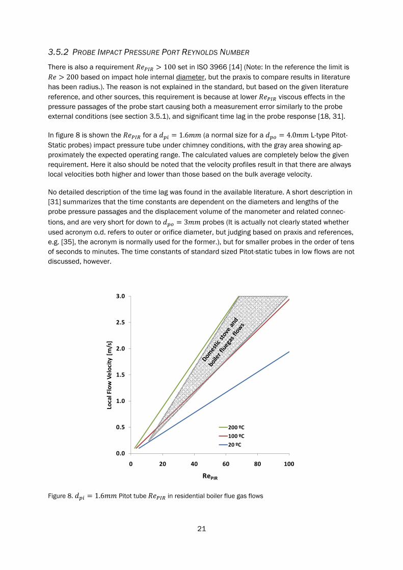
In figure 8 is shown the for a 1.6 (a normal size for a 4.0 L-type Pitot-Static probes) impact pressure tube under chimney conditions, with the gray area showing ap-proximately the expected operating range. The calculated values are completely below the given requirement. Here it also should be noted that the velocity profiles result in that there are always local velocities both higher and lower than those based on the bulk average velocity.

No detailed description of the time lag was found in the available literature. A short description in [31] summarizes that the time constants are dependent on the diameters and lengths of the probe pressure passages and the displacement volume of the manometer and related connec-tions, and are very short for down to 3 probes (It is actually not clearly stated whether used acronym o.d. refers to outer or orifice diameter, but judging based on praxis and references, e.g. [35], the acronym is normally used for the former.), but for smaller probes in the order of tens of seconds to minutes. The time constants of standard sized Pitot-static tubes in low flows are not discussed, however.

Figure 8. 1.6 Pitot tube in residential boiler flue gas flows

0.0

0.5

1.0

1.5

2.0

2.5

3.0

0 20 40 60 80 100

Local Flow Velocity [m/s]

RePIR

200 ºC

100 ºC

20 ºC

22

3.5.3 SIGNIFICANCE OF VISCOUS EFFECTS IN CHIMNEY FLOW MEASUREMENTS

Sections 3.5.1-3.5.2 and related reasoning implies that in residential boiler chimney flow condi-tions Pitot tubes (and other probes) are potentially suffering from significant enough viscous ef-fects to void the assumptions that justify the use of the quadratic Bernoulli correlation, a linear calibration coefficient, and the measurement uncertainties in ISO 10780 and ISO 3966. This is a clear implication that, under the given chimney conditions, differential pressure producing probes should always be calibrated in situ specifically for the intended operating range.

The impact of time lag caused by low of a standard Pitot-static tube could not be deter-mined based on available literature and the significance should thus be determined experimen-tally in the case of residential chimney flows.

3.6 WALL PROXIMITY AND STEM BLOCKAGE

To avoid blockage and pressure gradient errors in Pitot tube measurements in conduits the probe should not cause errors due to wall proximity, probe volume displacement (Venturi) effects, and pressure gradient displacement effects. In relatively small ducts these effects become significant as the probe size cannot be decreased easily. These effects cause generally an overestimation bias.

A dimensional limit of ⁄ 0.02 is set in ISO 3966, after which a correction should be done. In ISO 10780 this has been translated to an internal cross sectional area limit of 0.07 of the duct for the method to be valid, giving a minimum of 0.3 for round ducts. This is also in accordance with Ower [18] stating that an 8 Pitot probe should not be used in 0.3 ducts for traversing measurements.

Residential heating boiler flue gas ducts and chimneys range normally from 80 to 100 meaning that the ISO 10780 and ISO 3699 methods and uncertainties are not valid

as such regarding these requirements. ISO 3699 provides a correction method and a summary is given also in [20, 31]. As an example, if 0.5% maximum error of the differential pressure due to these effects is allowed, should not be greater than 1.6 for D80 and 2.0 for D100 chimneys. These probe sizes are not readily available and may start suffering from significant time lag in response, as stated earlier, and thus the normally used probes with 4 to

8 would require either theoretical error correction or in situ calibration.

3.7 FLUE GAS DENSITY

The fluid density is used both in the Bernoulli equation and when converting between volume and mass flow rates. According to ISO 10780 and ISO 3699 [13, 14] a correction for density has to be done if the gas density is suspected to be significantly different to that of air. Especially with wet biomass with moisture contents greater than 20% (wet basis) over +5% differences in density compared to air may occur, depending also on the combustion excess air ratio.

23

3.8 AVERAGE FLOW TEMPERATURE

During operation the flue gas temperature normally varies in the range of about 80…200ºC, and because the boilers often are modulating the combustion power, for dynamic measurements al-most the whole temperature range can be present across the previously mentioned range of

for D80 and D100 chimneys. During startup and stop sequences and leakage flows tem-peratures down to ambient will be present.

In the traversing method according to ISO 10780 [13] the absolute temperature of each meas-urement point should not differ more than 5% from the average absolute temperature in the measurement cross section. This translates to ±18ºC at 80ºC and ±24ºC at 200ºC average flue gas temperature.

In continuous dynamic measurements when traversing is not done care must be taken to meas-ure a representative average bulk temperature. Based on personal field and laboratory meas-urement experience of the author, the local temperatures in a flue gas duct can vary significantly (in extreme cases tens of ºC) over the cross section depending on various factors, such as dis-tance from the boiler outlet, boiler construction, insulation of the duct, combustion power modu-lation rate, flow type, and vertical or horizontal alignment of the duct. A temperature profile may be preserved for relatively long distances even in vertical ducts if the flow is partially laminar, and similarly to the velocity profile, the temperature profile can also change dependent on the flow rate and type. Thus for continuous dynamic measurements a single point temperature measure-ment may not be sufficient, if a consistent representative bulk average temperature cannot be confirmed for the whole operating range. Vertical ducts should be preferred to prevent natural density stratification due to heat losses through the walls.

The measurement error caused by a wrong bulk average temperature measurement (density de-termination error) is dependent on the temperature, such that the error decreases with increasing temperature. At 80ºC average bulk temperature a ±20ºC measurement error causes a ±2.9% error in the determination of the flow rate, while at 200ºC the same error is ±2.1%.

3.9 YAW ANGLE

Misalignment of the Pitot probe with respect to the flow direction (yaw angle) causes measure-ment errors [14, 18, 20], for which static tubes are more sensitive than total pressure tubes. For a Pitot-static probe a maximum of ±5% impact pressure deviation can be assumed within 30º yaw angle and less than +2% if the yaw angle is kept under 5º. These error estimations are under normal measurement conditions and it is mentioned that the they are slightly dependent on the

[14], but the sources do not specifically discuss the case of laminar flows, or cases where viscous effects may not be negligible.

A fixed stand with a locking system to fix the probe always in the same position is an easy and feasible solution for minimizing alignment errors in cases if the probe often needs to be taken out e.g. for cleaning.

24

3.10 VIBRATIONS

Errors because of probe vibration [18] are unlikely to disturb measurements in residential chim-ney conditions; Fluid flow velocities are not high enough to induce vibrations to the probe and devices causing significant enough mechanical vibrations transferred via duct walls are unlikely.

3.11 TURBULENCE

Turbulence may cause additional pressure difference sensed between the impact and static ports of the probe. Ower [18] summarizes that the turbulence intensities in industrial applications will have negligible effects.

3.12 DIFFERENTIAL PRESSURE MEASUREMENT

The flue gas flow from a normal residential heating boiler modulating its combustion power be-tween 30% and 100% of nominal results in a chimney flow velocity range of approximately from 1 to 3m/s, corresponding to differential pressures of 0.5 to 3.0Pa with standard Pitot-static probes. A resolution of less than 0.01Pa would be required to register useful data regarding small chang-es the flow velocity during dynamic measurements.

Commercially available pressure transducers intended for low differential pressures are normally calibrated for a range of up to tens of Pa with calibration points that have an uncertainty of ±0.2Pa or more. In addition a relative uncertainty is often given as a percentage of the range and covers uncertainties such as temperature drift, hysteresis, non-linearity, digital resolution, trans-ducer tilt etc. For example, a typical transducer with a range of 0 to 30Pa and an uncertainty of 2% of the range cannot be trusted to give useful data below a resolution of 0.6Pa.

However, the same pressure transducers often do produce a measurand correlated signal even at the very low differential pressures of chimney flue gas flows and may still be used if calibrated in a correct way, preferably in combination with the probe.

3.13 OTHER CONSIDERATIONS

Both the temperature range and chemical conditions in flue gases put requirements on the used sensor construction materials.

Flue gases from a boiler contain also particulate matter, soot and ash, which can easily clog the sensor. Condensing fluids, e.g. water and tar evaporated from the fuel, usually worsen the clog-ging. This sets requirements for being able to dismount, clean, and mount the sensor often and quickly without causing a need for recalibration. Preferably the cleaning should also be possible during boiler operation.

25

Heat conductance from the probe to the ambient should be minimized by material choice and insulation on the outside to prevent water vapor condensation from the flue gas flow on to the probe surface and condensation in the connecting tubes.

Especially in field conditions the flow measurement method should not cause a significant pres-sure drop, as this would most likely prevent a natural chimney draft based boiler from operating normally. Even in laboratory conditions it is beneficial to be able to use a method which causes only a low permanent pressure drop to the flow, both because of exhaust gas fan sizing needs and the possibility to emulate natural chimney draft conditions for a boiler.

For routine field testing of boilers the method should be inexpensive, reliable, and the device should be easy to mount and clean.

26

4 DISCUSSION AND CONCLUSIONS Single point dynamic velocity pressure measurements, such as the Pitot-static tube, are prone to significant errors in residential chimney conditions. Several requirements set in ISO 10780 and ISO 3966 are either met questionably or not met at all, meaning that the method and uncertain-ties defined in the standard are not valid as such. In all such cases the measurement method should be calibrated specifically to the application and its whole operating range, and preferably in situ.

A significant velocity profile change happens in the normal combustion power modulation range of a residential boiler, and during start and stop sequences. Velocity profiles at low flow rates are often practically difficult or impossible to measure because of e.g. burner controller or load limita-tions.

Not fully developed and/or skewed velocity profiles are practically unavoidable because the straight duct distances needed to always justify the assumption of fully developed velocity profiles are often practically not possible in laboratories and impossible in field conditions. The shorter distances used in practice means that measurements are done in the hydrodynamic entrance region, where the velocity profile is dependent on the , i.e. dependent on both flow velocity and temperature, which are constantly varying because non steady state operation of the boilers. In the case of disturbances, e.g. bends, the velocity profile may also change from skewed to al-most fully symmetric within the normal operating range of residential boilers when the flow type changes between turbulent and laminar.

Determination of the flow type within the turbulent to laminar transition region is practically im-possible without confirming with traversing velocity pressure measurements. In the transition region there may also be a hysteresis effect causing apparently random changes in the flow type, even with a constant flow rate, although this behavior seems unlikely in short chimneys.

There is thus risk for significant measurement errors with dynamic continuous single point meas-urements because of the velocity profile changes, depending on the positioning of the probe. If the used velocity profile is based on initial traversing measurements with high (turbulent) flow rates, then there will be a bias for overestimation of lower flow rates.

The low flow velocities during start and stop sequences, minimum combustion power, and leak-age flow measurements result in fluid viscous effects becoming significant enough to cause a voiding of a constant probe calibration coefficient. This effect may also result in a significant over estimation bias of the velocity pressure at low flow rates and must be accounted for by calibrating the probe for the specific operating conditions.

The probe size may become a significant factor in the relatively small ducts, causing blockage and wall proximity effects, which should be taken into account with an in situ calibration.

Care should also be taken with the temperature measurement needed for the density determina-tion for continuous flow rate measurements as the temperature of a single point may not repre-sent the bulk average temperature over the whole operating range. The error can be significant and an average of several temperatures over the cross section is preferable.

27

The presented characterization for residential boilers and the reported issues with industrial boil-ers imply that even boilers in between theses categories, such as block heating or small district heating applications, are potentially prone to similar errors.

The physical laws governing the probe response are also valid for other types of sensors using a differential pressure method, meaning that all such probes should be analyzed in a similar man-ner before use in residential chimneys.

The problems caused by the changing and often skewed velocity profiles could be taken into ac-count by using an averaging multi-port Pitot-static probe [24]. Research has been done in the area and commercial products are already available for some applications, such as ventilation or gas flow rate measurements. These probes cause a low pressure drop to the flow and can be designed to be easily inspected and cleaned.

28

5 ACKNOWLEDGMENTS This research project has been supported by a Marie Curie Early Stage Research Training Fellow-ship of the European Community’s Sixth Framework Programme under contract number MEST-CT-2005-020498, project SOLNET. The work was performed within the project SWX-Energi and fi-nanced by the European Union, Swedish Energy Agency, Region Dalarna and Region Gävleborg.

29

30

6 NOMENCLATURE

Duct internal cross section area Shape dependent parameter Shape dependent parameter

Probe outer diameter

Probe impact hole diameter Duct internal diameter Probe calibration coefficient

Velocity profile factor Probe outer radius

Probe impact hole radius Location on duct radius Duct internal radius Relative location on duct radius Reynolds number

based on and based on probe local and

based on probe local and Critical (transition between laminar and turbulent flow types)

Characteristic hydrodynamic measure (e.g. radius, diameter or length) ⁄ Fluid velocity ⁄ Fluid velocity at duct center axis ⁄ Fluid velocity at ⁄ Average fluid velocity over (average bulk velocity) ⁄ Fluid velocity at

⁄ Local velocity in laminar flow case ⁄ Local velocity in turbulent flow case

Length to achieve fully developed flow velocity profile Greek symbols

⁄ Fluid kinematic viscosity ⁄ Fluid density Δ Differential pressure (velocity pressure) Acronyms 80 Chimney with 80 100 Chimney with 100

31

32

7 REFERENCES

1. Olsson, M., Residential biomass combustion - emissions of organic compounds to air from wood pellets and other new alternatives, in Institutionen för kemi- och bioteknik, Skogsindustriell kemiteknik. 2006, Chalmers tekniska högskola. p. 200.

2. Boman, C., Particulate and Gaseous Emissions from Residential Biomass Combustion, in Teknisk-naturvetenskaplig fakultet. 2005, Umeå universitet: Umeå.

3. Hartmann, H., et al., Staubemissionen aus Holzfeuerungen - Einflussfaktoren und Be-stimmungsmethoden, in Berichte aus dem TFZ, T.-u.F. (TFZ), Editor. 2006: Straubing.

4. CEN, EN 303 - Heating boilers - Part 5: Heating boilers for solid fuels, hand and automati-cally stocked, nominal heat output of up to 300 kw - Terminology, requirements, testing and marking. 1999, European Comittee for Standardization.

5. Fiedler, F., Combined solar and pellet heating systems : Studies of energy use and CO-emissions. 2006, Mälardalen University: Västerås. p. 204.

6. Kunde, R., et al., Felduntersuchungen an Holzpellet-Zentralheizkesseln. Das Energie-Fachmagazin BWK, 2009(1/2009): p. 58-66.

7. Ulrik Pettersson, M.J., Henrik Persson, FBT-04/24 - Låglastkaraktäristik i små pelletsan-läggningar. 2004: p. 19.

8. Haller, M.Y., et al., A unified model for the simulation of oil, gas and biomass space heat-ing boilers for energy estimating purposes. Part I: Model development. Journal of Building Performance Simulation, 2010. 4(1): p. 1-18.

9. Haller, M.Y., et al., A unified model for the simulation of oil, gas and biomass space heat-ing boilers for energy estimating purposes. Part II: Parameterization and comparison with measurements. Journal of Building Performance Simulation, 2010. 4(1): p. 19-36.

10. Persson, T., Combined solar and pellet heating systems for single-family houses : -How to achieve decreased electricity usage, increased system efficiency and increased solar gains. 2006, Department of Energy and Environmental Technology, KTH - Royal Institute of Technology: Stockholm.

11. Thiers, S., B. Aoun, and B. Peuportier, Experimental characterization, modeling and simu-lation of a wood pellet micro-combined heat and power unit used as a heat source for a residential building. Energy and Buildings, 2010. 42(6): p. 896-903.

12. CEN, EN 12952 - Water-tube boilers and auxiliary installations - Part 15: Acceptance tests. 2003, European Comittee for Standardization.

13. ISO, ISO 10780:1994(E) - Stationary source emissions - Measurement of velocity and volume flowrate of gas streams in ducts, I.O.f. Standardization, Editor. 1994, International Organization for Standardization.

14. ISO, ISO 3966:2008(E) - Measurement of fluid flow in closed conduits - Velocity area methods using Pitot static tubes, I.O.f. Standardization, Editor. 2006, International Organ-ization for Standardization.

15. Robinson, R.A., Problems with Pitots - Issues with flow measurement in stacks, in Interna-tion Environmental Technology (IET). 2004.

16. Dobrowolski, B., M. Kabacinski, and J. Pospolita, A mathematical model of the self-averaging Pitot tube. A mathematical model of a flow sensor. Flow Measurement and In-strumentation, 2005. 16(4): p. 251-265.

33

17. Leland, B.J., et al., Correction of S type pitot static tube coefficients when used for isoki-netic sampling from stationary sources. Environmental Science and Technology, 1977. 11(7): p. 694-700.

18. Ower, E. and R.C. Pankhurst, The measurement of air flow. 5th revised edition ed. 1977: Pergamon Press.

19. Boetcher, S.K.S. and E.M. Sparrow, Limitations of the standard Bernoulli equation method for evaluating Pitot/impact tube data. International Journal of Heat and Mass Transfer, 2007. 50(3-4): p. 782-788.

20. Folsom, R.L., Review of the Pitot Tube. Transactions of the ASME, 1956. 78: p. 1447-1460.

21. Spitzer, D.W., Industrial flow measurement. 2. ed. ed, ed. D.W. Spitzer. 1990, Research Triangle Park, N.C. :: Instrument Society of America. 441.

22. Spitzer, D.W., Flow measurement. Practical guides for measurement and control, ed. D.W. Spitzer. 1991, Research Triangle Park, NC: Instrument Society of America.

23. Incropera, F.P. and D.B. Dewitt, Fundamentals of heat and mass transfer / Frank Incrope-ra, David Dewitt. 4. ed. ed. 1996, New York: Wiley. 886 s. :.

24. Taylor, J.C., Flow measurement by self-averaging Pitot-tubes. Measurement and Control, 1988. 20(10 , Dec. 1987-Jan. 1988): p. 145-147.

25. Wagner, W., Wärmeübertragung. 2. revised ed. ed. Vogel Fachbuch. 1988, Würzburg: Vogel.

26. Massey, B.S., Mechanics of Fluids. 6th ed. ed. 1989, London: Chapman & Hall. 599.

27. Schlichting, H. and K. Gersten, Boundary layer theory. 8th edition 2000, corrected printing 2003 ed. 2000, Berlin: Springer. 799.

28. Nyquist, G., Flödesmätningar med pitotrör – Provningsjämförelse 2002, ITM rapport 115, in ITM reports. 2003, Institutet för tillämpad miljöforskning: Stockholm.



31. Chue, S.H., Pressure probes for fluid measurement. Progresses in Aerospace Science, 1975. 16(2): p. 147-223.

32. Hurd, C.W., K.P. Chesky, and A.H. Shapiro, Influence of viscous effects on impact tubes. J. Appl. Mech., 1953. 248: p. 253-256.

33. MacMillan, F.A., Viscous effects on Pitot tubes at low speeds. J. R. Aero. Soc., 1954. 58: p. 837-839.

34. Lester, W.G.S., The flow past a pitot tube at low Reynolds numbers. Aeronautical Re-search Council Reports and Memoranda, 1961. R&M(3240).

35. Cooke, J.R., The use of quartz in the manufacture of small diameter pitot tubes. Aeronau-tical Research Council Current Papers, 1955. C.P.(190).

Documents

Characterization of residential chimney conditions for flue