1

Characterization of Cavitation Fields from Measured Pressure

Signals of Cavitating Jets and Ultrasonic Horns By

Sowmitra Singh1, Jin-Keun Choi, and Georges L. Chahine

DYNAFLOW, INC.

10621-J Iron Bridge Road, Jessup, Maryland 20794

ABSTRACT

Cavitation pressure fields under a cavitating jet and an ultrasonic horn were recorded for

different conditions using high frequency response pressure transducers. This aimed at

characterizing the impulsive pressures generated by cavitation at different intensities. The

pressure signals were analyzed and statistics of the amplitudes and widths of the impulsive

pressure peaks were extracted. Plots of number densities and cumulative numbers of peaks as

functions of peak amplitude, peak width, and the power of the ultrasonic horn or the jet were

generated. The analysis revealed the dominance of pulses with smaller amplitudes and larger

durations at lower cavitation intensities and the increase of the amplitudes and reduction of the

pulse widths at higher intensities. The ratio of the most probable peak amplitude to peak width

was computed. A representative Gaussian curve was then generated for each signal using a

characteristic peak amplitude and the corresponding most probable peak duration/width. This

resulted in a proposed statistical representation of a cavitation field, useful to characterize

cavitation fields of various intensities.

1. INTRODUCTION

Prediction of cavitation erosion on propellers, ship structures, and in general on any

structure subjected to cavitation is of great interest to many industries. However, this task is often

difficult and selection of new materials or material protection coatings that are cavitation erosion

resistant is instead most often based on laboratory testing using accelerated erosion methods.

These aim at comparing within short time periods the resistance of a new material relative to

other standard materials. Erosion in the real field occurs over long durations of exposure, while

accelerated erosion tests, by definition, involve subjecting the material to an erosion field that is

significantly more “intense” than the actual cavitation that the studied material will be subjected

to. The validity of such an approach is however not obvious, as it has been observed that the

relative resistance of two materials can be different at different “intensities” of cavitation [1,2].

However, the definition of cavitation “intensity” is not universal. One classical definition [3, 4]

using an integral quantity is based on a concept similar to that of the acoustic intensity. This

expresses the cavitation intensity at a selected point on the material subjected to cavitation as,

2

1

(1/ )N

i ic P t , where N is the total number per unit time of impulsive loads of amplitude iP

1 Author to whom correspondence should be addressed. Electronic mail:sowmitra@dynaflow-

inc.com

2

and duration iΔt ; is the liquid density, c is the sound speed in the liquid and c is the liquid

acoustic impedance. With this definition, an infinite number of configurations can result in the

same intensity; namely one can achieve in an accelerated erosive test the same intensity by

either increasing the amplitude of the impulsive loads, iP , for the same N , or increasing the

frequency, N , for the same iP . It is however, obvious, from the material response viewpoint that

these two acceleration types may not result in the same outcome. For instance increasing a lot

the frequency while using an amplitude well below the material limit strength will not result in

any significant damage, while a few blows well above the material limit strength will. In this

paper, we aim at developing an understanding of the distribution of impulsive loads

characteristics of the two popular accelerated erosion testing methods: the cavitating jet method

(e.g. ASTM G134 standard [5]) and the ultrasonic method (i.e. ASTM G32 standard [5]) in order

to develop the knowledge base needed to conduct intelligent well-controlled tests. Such a

characterization should also enable a better description of the degree or level of advancement of

cavitation in a given flow field.

Any cavitation field, irrespective of its configuration and origin can be described as being

comprised of numerous individual cavitation events; each event corresponding to the explosive

volume growth and violent collapse of single or multiple bubbles or bubble clouds. These events

are known to be accompanied with sharp pressure peaks and impulsive loads on nearby

structures are well-known since the early works of Besant in 1859 [6] and Lord Rayleigh in 1917

[7] on isolated bubbles. More recently, the dynamics of bubble clouds have been shown to result

in extremely high pressures and intense erosion. This is presently recognized as the most

aggressive or erosive form of cavitation and has been the subject of many studies starting with

the pioneering works of Mørch [8], d’Agostino and Brennen [9], and Chahine [10]. These studies

have shown that bubble collective effects in the cloud result in much enhanced bubble collapse

pressures exerted over longer periods of time. Cloud cavitation has been extensively studied

since then; see for example [11-13].

In order to study cavitation erosion in a controlled environment and in an accelerated

manner, several laboratory techniques to generate cavitation have been devised by the

community. These techniques involve the utilization of ultrasonic vibration to generate the

cavitation, cavitation flow loops with strong separating flows, rotating disks, vortex generators,

and submerged cavitating jets. Ultrasonic horns are used to generate cavitation on sample

material surfaces and have significant applications in material cavitation erosion resistance

testing [14-16]. Ultrasonic horns typically have a fixed vibration frequency but variable vibratory

amplitude. The advantage of these vibratory systems is that they can generate cavitation erosion

in a quiescent liquid. The cavitating jet technique is also popular due to its flexibility of adjusting

in a wide range the cavitation intensity [17-21]. Some of the afore described techniques were

standardized and resulted in American Society for Testing and Materials (ASTM) Standards such

as G-32 “Test Method for Cavitation Erosion Using Vibratory Apparatus” and G-134 “Test

Method for Erosion of Solid Materials by a Cavitating Liquid Jet” [5].

In this paper, we describe our study on the cavitation intensity of various cavitation fields

generated by an acoustic horn [5] and by a CAVIJET® [22] cavitating jets at various driving

pressures by carrying out pressure measurements directly under the cavitation field. The erosive

3

potential or cavitation intensity under the cavitating jet and a vibrating horn were assessed by

correlating their intensities with the recorded pressure pulses. Being able to understand and

characterize the cavitation fields of these controllable devices will provide an insight into how to

characterize other more complex cavitation fields, such as cavitation in turbomachines or on

propeller blades. In the end, proper characterization of the cavitation environment for various

cavitation fields from laboratory scale to full scale will enable us to predict full scale cavitation

erosion from erosion in laboratory tests.

2. FACILITY AND INSTRUMENTATION

Two accelerated erosion testing facilities have been used in this study namely, an

ultrasonic cavitation test facility and DYNAFLOW’S cavitating jets testing facility.

In ultrasonic cavitation tests, the cavitation is generated by a vibratory device employing

a magnetostrictive ultrasonic horn. The high frequency oscillations of the horn induce cyclic

formation of very high and very low pressures, generate high tension in the liquid during a

negative pressure cycle that result in bubble growth followed by strong bubble cloud collapse

during the positive pressure cycle. A sample “button” of the material being tested is affixed to

the end of the horn and is subjected to cavitation resulting from the vibrations of the horn. A

cavitation hemispherical cloud forms at the tip of the horn and results in progressive damage to

the sample [8]. The ASTM G32 -09 [5] specifies the sample diameter, 16 mm, the vibration

frequency, 20 kHz, and amplitude, 50 m peak-to-peak (calibrated using a bifilar microscope),

and the shape and size of the container in order to avoid variations between tests and laboratories

due to acoustic interaction between transducer and container. We used a 2,000 ml beaker filled

with distilled water. The tip of the horn is submerged 8 mm. beneath the free surface. In addition,

the temperature is controlled by immersing the beaker in a water bath maintained at 25°C ±2 ºC.

In an “alternative” test configuration that we usually employ with composite materials which are

difficult to be made into threaded buttons, the horn tip is placed at a small distance from a

stationary material sample, typically a distance of 0.5 mm, and a cylindrical cavitation cloud [8]

is generated between the sample and the face of the tip of the horn made of a strongly cavitation

resistant “button” (e.g. Titanium). Figure 1 shows examples of advanced erosion patterns with

the two ultrasonic cavitation methods. In the present study, the location of the sample for the

alternative method is where the pressure transducer is placed to record signals of a corresponding

cavitation field.

For both methods, when using the same vibration frequency, as is the case in the paper,

cavitation severity is indicated by the amplitude of the oscillations or the power input to the

ultrasonic horn.

4

Figure 1. Ultrasonic technique eroded samples pictures. Left: Tested G32 metallic button

sample; Right: eroded composite material sample from the alternative G32 method. Sample distance

from horn = 0.5 mm, approximate diameter of erosion pattern = 1.3 mm.

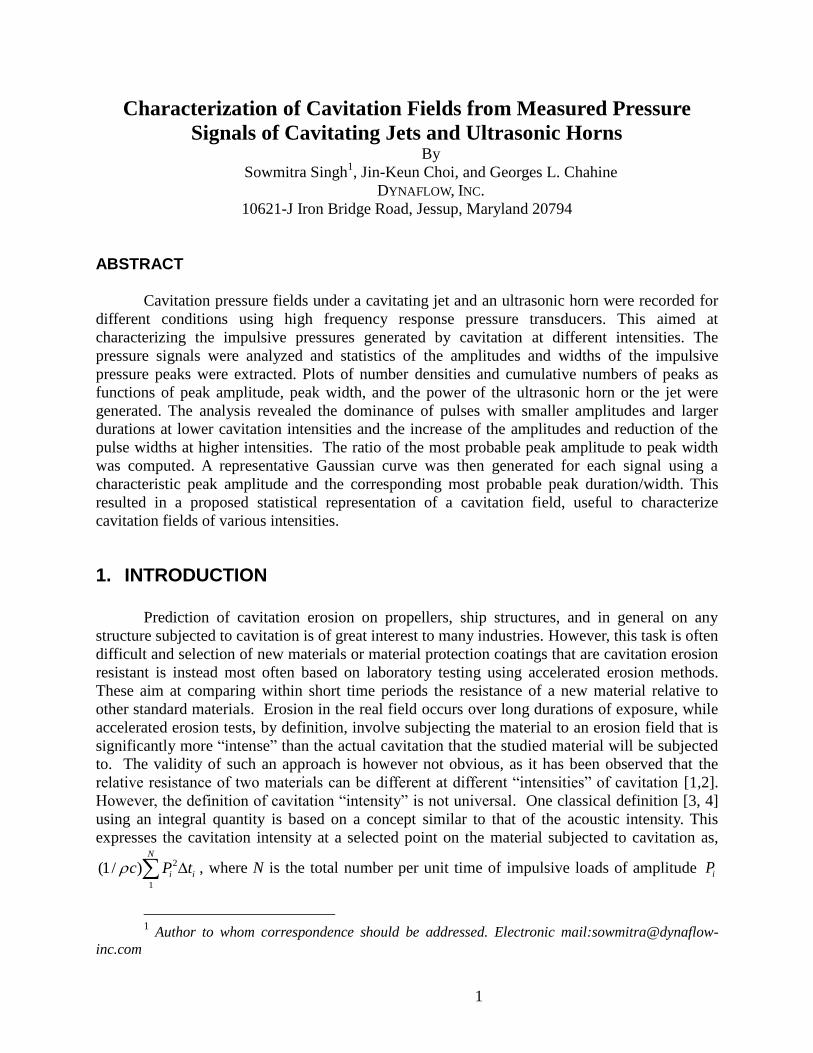
In submerged liquid jets, cavitation occurs in the shear layer between the high speed liquid

in the jet and the host liquid [22,23] . The intensity of the cavitation produced by the cavitating

jet can be varied in a very wide range through adjustment of the jet velocity and the ambient

pressure in which the jet is discharged. This flexibility makes a cavitating jet a great research and

testing tool to study parametrically the effect of cavitation intensity on material behavior since

the testing time and the other jet parameters can be adjusted to provide either quick erosion for

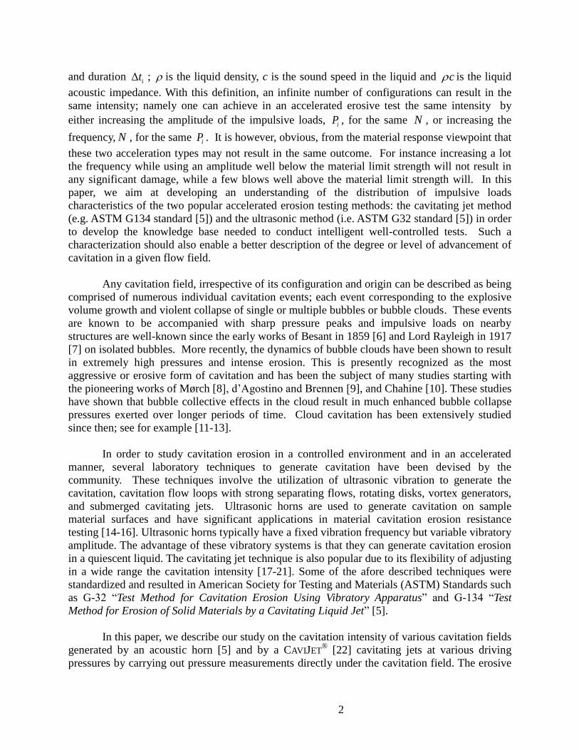
initial screening or time-accelerated erosion. A typical picture of the cavitation in the shear layer

of a CAVIJET®

is shown in Figure 2, and typical cavitation patterns on materials can be seen in

Figure 3.

a Figure 2. Cavitation pattern in the shear layer of a CAVIJET

® nozzle (Visualizations conducted

with a very large 50 mm diameter nozzle).

Figure 3. Cavitation erosion pattern on metals created by a cavitating jet. Jet diameter = 1.17

mm. Sample distance from jet = 13.97 mm, approximate diameter of erosion pattern = 5 mm.

5

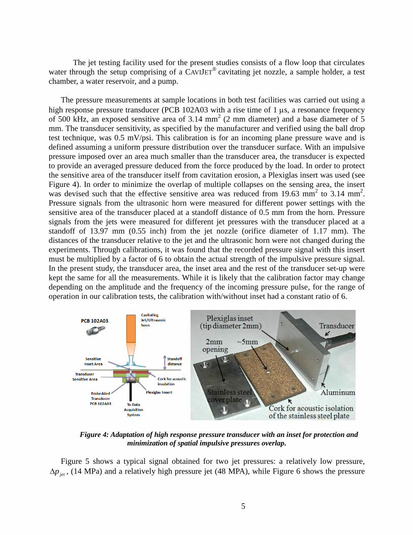
The jet testing facility used for the present studies consists of a flow loop that circulates

water through the setup comprising of a CAVIJET®

cavitating jet nozzle, a sample holder, a test

chamber, a water reservoir, and a pump.

The pressure measurements at sample locations in both test facilities was carried out using a

high response pressure transducer (PCB 102A03 with a rise time of 1 s, a resonance frequency

of 500 kHz, an exposed sensitive area of 3.14 mm2 (2 mm diameter) and a base diameter of 5

mm. The transducer sensitivity, as specified by the manufacturer and verified using the ball drop

test technique, was 0.5 mV/psi. This calibration is for an incoming plane pressure wave and is

defined assuming a uniform pressure distribution over the transducer surface. With an impulsive

pressure imposed over an area much smaller than the transducer area, the transducer is expected

to provide an averaged pressure deduced from the force produced by the load. In order to protect

the sensitive area of the transducer itself from cavitation erosion, a Plexiglas insert was used (see

Figure 4). In order to minimize the overlap of multiple collapses on the sensing area, the insert

was devised such that the effective sensitive area was reduced from 19.63 mm2 to 3.14 mm

2.

Pressure signals from the ultrasonic horn were measured for different power settings with the

sensitive area of the transducer placed at a standoff distance of 0.5 mm from the horn. Pressure

signals from the jets were measured for different jet pressures with the transducer placed at a

standoff of 13.97 mm (0.55 inch) from the jet nozzle (orifice diameter of 1.17 mm). The

distances of the transducer relative to the jet and the ultrasonic horn were not changed during the

experiments. Through calibrations, it was found that the recorded pressure signal with this insert

must be multiplied by a factor of 6 to obtain the actual strength of the impulsive pressure signal.

In the present study, the transducer area, the inset area and the rest of the transducer set-up were

kept the same for all the measurements. While it is likely that the calibration factor may change

depending on the amplitude and the frequency of the incoming pressure pulse, for the range of

operation in our calibration tests, the calibration with/without inset had a constant ratio of 6.

Figure 4: Adaptation of high response pressure transducer with an inset for protection and

minimization of spatial impulsive pressures overlap.

Figure 5 shows a typical signal obtained for two jet pressures: a relatively low pressure,

jetp , (14 MPa) and a relatively high pressure jet (48 MPA), while Figure 6 shows the pressure

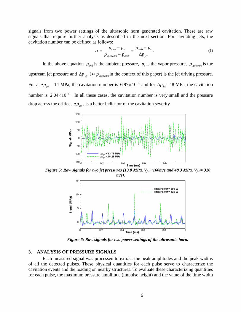
6

signals from two power settings of the ultrasonic horn generated cavitation. These are raw

signals that require further analysis as described in the next section. For cavitating jets, the

cavitation number can be defined as follows:

amb v amb v

upstream amb jet

p p p p

p p p

. (1)

In the above equation ambp is the ambient pressure, vp is the vapor pressure, upstreamp is the

upstream jet pressure and jetp (

upstreamp in the context of this paper) is the jet driving pressure.

For a jetp = 14 MPa, the cavitation number is 36.97 10 and for

jetp =48 MPa, the cavitation

number is 32.04 10 . In all these cases, the cavitation number is very small and the pressure

drop across the orifice, jetp , is a better indicator of the cavitation severity.

Figure 5: Raw signals for two jet pressures (13.8 MPa, Vjet ~160m/s and 48.3 MPa, Vjet = 310

m/s).

Figure 6: Raw signals for two power settings of the ultrasonic horn.

3. ANALYSIS OF PRESSURE SIGNALS

Each measured signal was processed to extract the peak amplitudes and the peak widths

of all the detected pulses. These physical quantities for each pulse serve to characterize the

cavitation events and the loading on nearby structures. To evaluate these characterizing quantities

for each pulse, the maximum pressure amplitude (impulse height) and the value of the time width

7

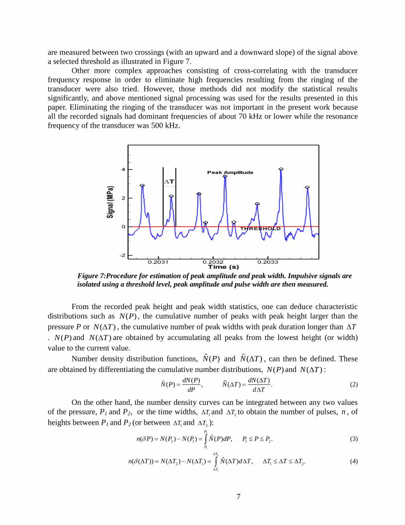
are measured between two crossings (with an upward and a downward slope) of the signal above

a selected threshold as illustrated in Figure 7.

Other more complex approaches consisting of cross-correlating with the transducer

frequency response in order to eliminate high frequencies resulting from the ringing of the

transducer were also tried. However, those methods did not modify the statistical results

significantly, and above mentioned signal processing was used for the results presented in this

paper. Eliminating the ringing of the transducer was not important in the present work because

all the recorded signals had dominant frequencies of about 70 kHz or lower while the resonance

frequency of the transducer was 500 kHz.

Figure 7:Procedure for estimation of peak amplitude and peak width. Impulsive signals are

isolated using a threshold level, peak amplitude and pulse width are then measured.

From the recorded peak height and peak width statistics, one can deduce characteristic

distributions such as ( )N P , the cumulative number of peaks with peak height larger than the

pressure P or ( )N T , the cumulative number of peak widths with peak duration longer than T

. ( )N P and ( )N T are obtained by accumulating all peaks from the lowest height (or width)

value to the current value.

Number density distribution functions, ( )N P and ( )N T , can then be defined. These

are obtained by differentiating the cumulative number distributions, ( )N P and ( )N T :

( ) ( )( ) , ( ) .

dN P dN TN P N T

dP d T

(2)

On the other hand, the number density curves can be integrated between any two values

of the pressure, P1 and P2, or the time widths, 1T and

2T to obtain the number of pulses, n , of

heights between P1 and P2 (or between 1T and

2T ):

2

1

2 1 1 2( ) ( ) ( ) ( ) , .

P

P

n P N P N P N P dP P P P (3)

2

1

2 1 1 2( ( )) ( ) ( ) ( ) , .

T

T

n T N T N T N T d T T T T

(4)

8

A two-dimensional number density distribution can also be defined encompassing the

variations of both the peak height, P, and the peak width, T . The number of pulses occurring

within a peak width range, 2 1( )T T T , and a peak height range,

2 1P P P , can then be

given as follows:

2 2

1 1

( , ( )) ( , ) .

P T

P T

n P T N P T dPd T

(5)

To obtain the one-dimensional or two-dimensional number density distributions, N .

numerically, the entire range over which the peaks occur is divided into bins, P or ( )T , in

one dimension or ( )P T in two dimensions) and the number of pulses occurring within each

bin is counted, ( )n P or ( ( ))n T , in one dimension or ( , ( ))n P T in two dimensions. This

number is then normalized by the bin size to obtain the number density at discrete locations.

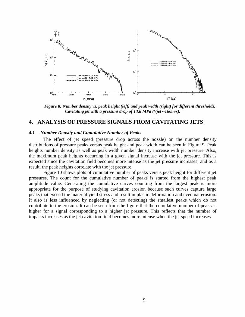
3.1 Effect of Pressure Threshold on Pressure Peak Statistics

Figure 8 illustrates the above described analysis for a cavitating jet operated at a pressure

of jetp = 13.8 MPa (Vjet ~160m/s). The figure shows number density distributions versus peak

height, ( )N P , and peak width, ( )N T , for different pressure threshold values. The number

density distribution versus peak height remains almost unaffected by the choice of the threshold,

except at very low peak height values, where smaller peak heights become excluded when a

higher threshold values are used. This trend of the curves at low peak height values is not an

issue, because the lowest amplitude pulses are of the order of signal noise and are mostly too

weak to contribute to cavitation erosion.

The number density distribution versus peak width, ( )N T , is more sensitive to the

chosen threshold. Naturally, because of the quasi-triangular shape of the pressure pulses,

choosing a higher threshold results in smaller time widths of the pulses detected, i.e., as seen in

Figure 8-right the distribution moves slightly to the left. This is a result of the peak duration

becoming shorter as the threshold becomes higher. However, it should be noted that the overall

trend is not affected much by the choice of the threshold.

9

Figure 8: Number density vs. peak height (left) and peak width (right) for different thresholds,

Cavitating jet with a pressure drop of 13.8 MPa (Vjet ~160m/s).

4. ANALYSIS OF PRESSURE SIGNALS FROM CAVITATING JETS

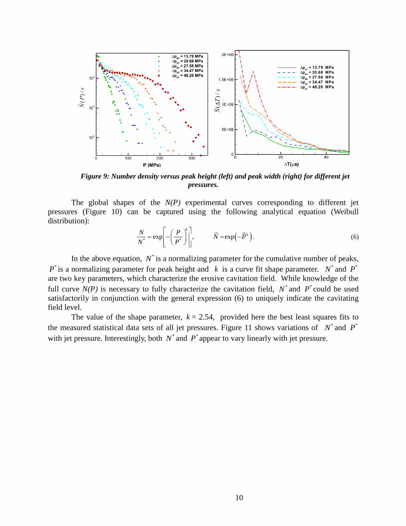
4.1 Number Density and Cumulative Number of Peaks

The effect of jet speed (pressure drop across the nozzle) on the number density

distributions of pressure peaks versus peak height and peak width can be seen in Figure 9. Peak

heights number density as well as peak width number density increase with jet pressure. Also,

the maximum peak heights occurring in a given signal increase with the jet pressure. This is

expected since the cavitation field becomes more intense as the jet pressure increases, and as a

result, the peak heights correlate with the jet pressure.

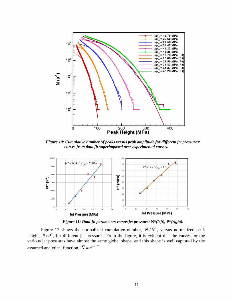
Figure 10 shows plots of cumulative number of peaks versus peak height for different jet

pressures. The count for the cumulative number of peaks is started from the highest peak

amplitude value. Generating the cumulative curves counting from the largest peak is more

appropriate for the purpose of studying cavitation erosion because such curves capture large

peaks that exceed the material yield stress and result in plastic deformation and eventual erosion.

It also is less influenced by neglecting (or not detecting) the smallest peaks which do not

contribute to the erosion. It can be seen from the figure that the cumulative number of peaks is

higher for a signal corresponding to a higher jet pressure. This reflects that the number of

impacts increases as the jet cavitation field becomes more intense when the jet speed increases.

10

Figure 9: Number density versus peak height (left) and peak width (right) for different jet

pressures.

The global shapes of the N(P) experimental curves corresponding to different jet

pressures (Figure 10) can be captured using the following analytical equation (Weibull

distribution):

* *exp , exp

k

kN PN P

N P

. (6)

In the above equation, *N is a normalizing parameter for the cumulative number of peaks, *P is a normalizing parameter for peak height and k is a curve fit shape parameter. *N and *P

are two key parameters, which characterize the erosive cavitation field. While knowledge of the

full curve N(P) is necessary to fully characterize the cavitation field, *N and *P could be used

satisfactorily in conjunction with the general expression (6) to uniquely indicate the cavitating

field level.

The value of the shape parameter, k = 2.54, provided here the best least squares fits to

the measured statistical data sets of all jet pressures. Figure 11 shows variations of *N and *P

with jet pressure. Interestingly, both *N and *P appear to vary linearly with jet pressure.

11

Figure 10: Cumulative number of peaks versus peak amplitude for different jet pressures:

curves from data fit superimposed over experimental curves.

Figure 11: Data-fit parameters versus jet pressure: N*(left), P*(right).

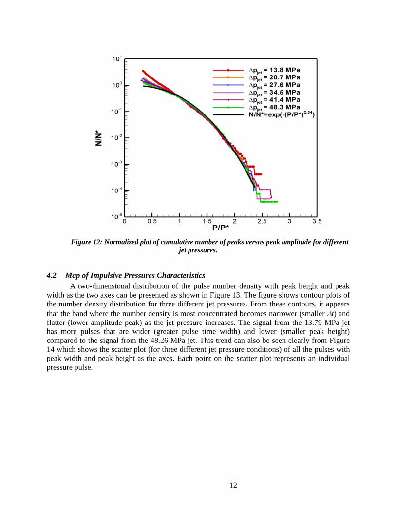
Figure 12 shows the normalized cumulative number, N / *N , versus normalized peak

height, P / *P , for different jet pressures. From the figure, it is evident that the curves for the

various jet pressures have almost the same global shape, and this shape is well captured by the

assumed analytical function, 2.54PN e .

12

Figure 12: Normalized plot of cumulative number of peaks versus peak amplitude for different

jet pressures.

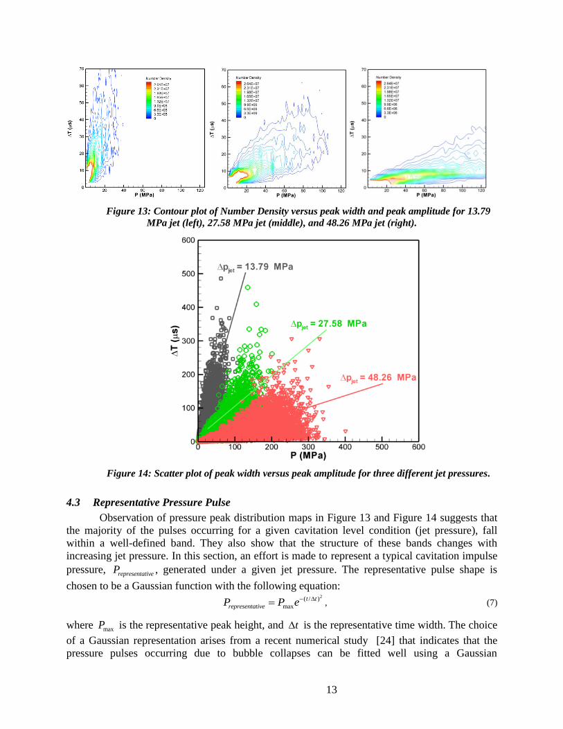
4.2 Map of Impulsive Pressures Characteristics

A two-dimensional distribution of the pulse number density with peak height and peak

width as the two axes can be presented as shown in Figure 13. The figure shows contour plots of

the number density distribution for three different jet pressures. From these contours, it appears

that the band where the number density is most concentrated becomes narrower (smaller t) and

flatter (lower amplitude peak) as the jet pressure increases. The signal from the 13.79 MPa jet

has more pulses that are wider (greater pulse time width) and lower (smaller peak height)

compared to the signal from the 48.26 MPa jet. This trend can also be seen clearly from Figure

14 which shows the scatter plot (for three different jet pressure conditions) of all the pulses with

peak width and peak height as the axes. Each point on the scatter plot represents an individual

pressure pulse.

13

Figure 13: Contour plot of Number Density versus peak width and peak amplitude for 13.79

MPa jet (left), 27.58 MPa jet (middle), and 48.26 MPa jet (right).

Figure 14: Scatter plot of peak width versus peak amplitude for three different jet pressures.

4.3 Representative Pressure Pulse

Observation of pressure peak distribution maps in Figure 13 and Figure 14 suggests that

the majority of the pulses occurring for a given cavitation level condition (jet pressure), fall

within a well-defined band. They also show that the structure of these bands changes with

increasing jet pressure. In this section, an effort is made to represent a typical cavitation impulse

pressure, representativeP , generated under a given jet pressure. The representative pulse shape is

chosen to be a Gaussian function with the following equation:

2( / )

max

t t

representativeP P e , (7)

where maxP is the representative peak height, and t is the representative time width. The choice

of a Gaussian representation arises from a recent numerical study [24] that indicates that the

pressure pulses occurring due to bubble collapses can be fitted well using a Gaussian

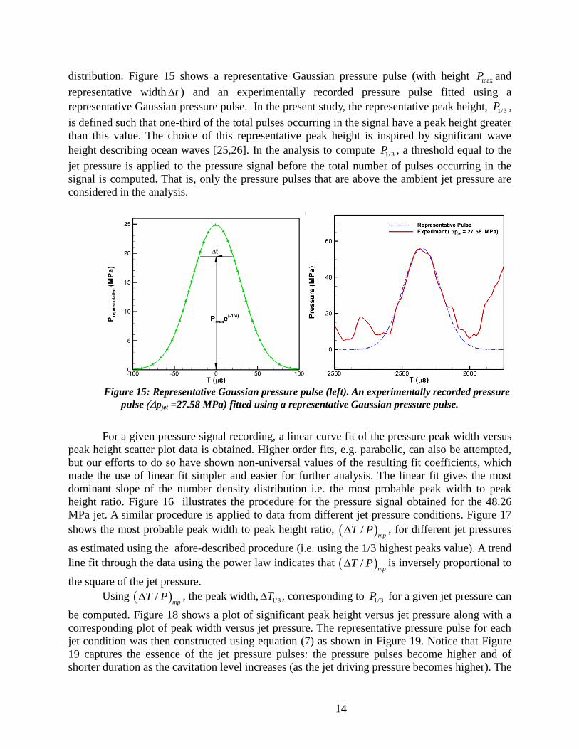
14

distribution. Figure 15 shows a representative Gaussian pressure pulse (with height maxP and

representative width t ) and an experimentally recorded pressure pulse fitted using a

representative Gaussian pressure pulse. In the present study, the representative peak height, 1/3P ,

is defined such that one-third of the total pulses occurring in the signal have a peak height greater

than this value. The choice of this representative peak height is inspired by significant wave

height describing ocean waves [25,26]. In the analysis to compute 1/3P , a threshold equal to the

jet pressure is applied to the pressure signal before the total number of pulses occurring in the

signal is computed. That is, only the pressure pulses that are above the ambient jet pressure are

considered in the analysis.

Figure 15: Representative Gaussian pressure pulse (left). An experimentally recorded pressure

pulse pjet =27.58 MPa) fitted using a representative Gaussian pressure pulse.

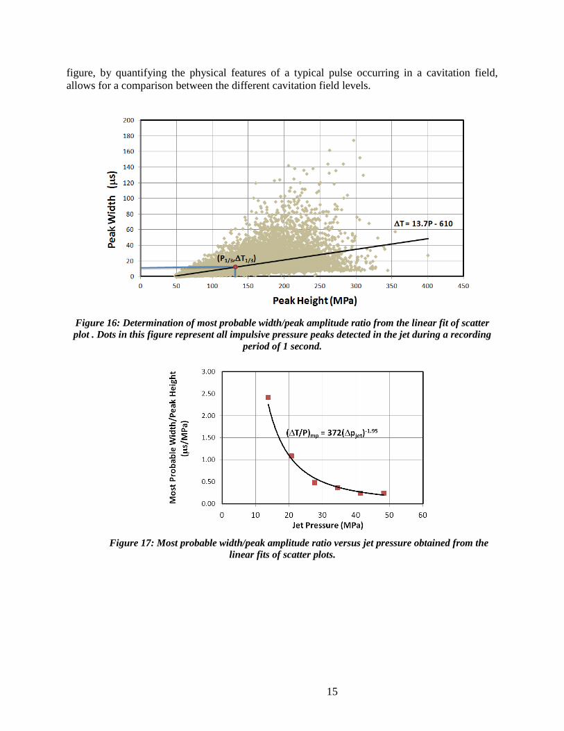
For a given pressure signal recording, a linear curve fit of the pressure peak width versus

peak height scatter plot data is obtained. Higher order fits, e.g. parabolic, can also be attempted,

but our efforts to do so have shown non-universal values of the resulting fit coefficients, which

made the use of linear fit simpler and easier for further analysis. The linear fit gives the most

dominant slope of the number density distribution i.e. the most probable peak width to peak

height ratio. Figure 16 illustrates the procedure for the pressure signal obtained for the 48.26

MPa jet. A similar procedure is applied to data from different jet pressure conditions. Figure 17

shows the most probable peak width to peak height ratio, /mp

T P , for different jet pressures

as estimated using the afore-described procedure (i.e. using the 1/3 highest peaks value). A trend

line fit through the data using the power law indicates that /mp

T P is inversely proportional to

the square of the jet pressure.

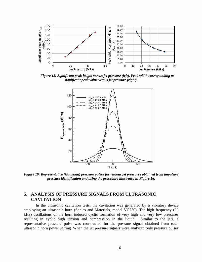
Using /mp

T P , the peak width, 1/3T , corresponding to 1/3P for a given jet pressure can

be computed. Figure 18 shows a plot of significant peak height versus jet pressure along with a

corresponding plot of peak width versus jet pressure. The representative pressure pulse for each

jet condition was then constructed using equation (7) as shown in Figure 19. Notice that Figure

19 captures the essence of the jet pressure pulses: the pressure pulses become higher and of

shorter duration as the cavitation level increases (as the jet driving pressure becomes higher). The

15

figure, by quantifying the physical features of a typical pulse occurring in a cavitation field,

allows for a comparison between the different cavitation field levels.

Figure 16: Determination of most probable width/peak amplitude ratio from the linear fit of scatter

plot . Dots in this figure represent all impulsive pressure peaks detected in the jet during a recording

period of 1 second.

Figure 17: Most probable width/peak amplitude ratio versus jet pressure obtained from the

linear fits of scatter plots.

16

Figure 18: Significant peak height versus jet pressure (left). Peak width corresponding to

significant peak value versus jet pressure (right).

Figure 19: Representative (Gaussian) pressure pulses for various jet pressures obtained from impulsive

pressure identification and using the procedure illustrated in Figure 16.

5. ANALYSIS OF PRESSURE SIGNALS FROM ULTRASONIC

CAVITATION

In the ultrasonic cavitation tests, the cavitation was generated by a vibratory device

employing an ultrasonic horn (Sonics and Materials, model VC750). The high frequency (20

kHz) oscillations of the horn induced cyclic formation of very high and very low pressures

resulting in cyclic high tension and compression in the liquid. Similar to the jets, a

representative pressure pulse was constructed for the pressure signal obtained from each

ultrasonic horn power setting. When the jet pressure signals were analyzed only pressure pulses

17

above the corresponding jet pressure were considered. A similar physically meaningful threshold

for noise removal was sought for each ultrasonic horn signal.

The fluid particle displacement in an acoustic field created by a vibratory horn, x , can be

given by:

sin(2 ),ox x ft (8)

where ox is the amplitude of the horn motion, and f is the vibratory frequency of the horn.

Differentiating the above equation, we can arrive at the particle velocity, u , in the acoustic field

immediately next to the horn tip:

2 cos(2 ).ou fx ft (9)

The acoustic pressure there can then be obtained by taking the product of the particle

velocity and acoustic impedance of the medium:

2 cos(2 ).op cu cfx ft (10)

Here, is the density of the medium, and c is the sound speed in the medium. For each signal,

the amplitude of the acoustic pressure is used as the threshold for analyzing the number of

pressure pulses occurring in the signal. This choice of threshold can be justified because any

impact pressure lower than the ambient acoustic pressure from the vibrating horn should be

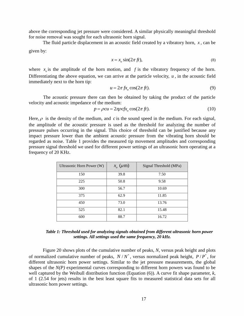
regarded as noise. Table 1 provides the measured tip movement amplitudes and corresponding

pressure signal threshold we used for different power settings of an ultrasonic horn operating at a

frequency of 20 KHz.

Ultrasonic Horn Power (W) ( m)ox Signal Threshold (MPa)

150 39.8 7.50

225 50.8 9.58

300 56.7 10.69

375 62.9 11.85

450 73.0 13.76

525 82.1 15.48

600 88.7 16.72

Table 1: Threshold used for analyzing signals obtained from different ultrasonic horn power

settings. All settings used the same frequency, 20 kHz.

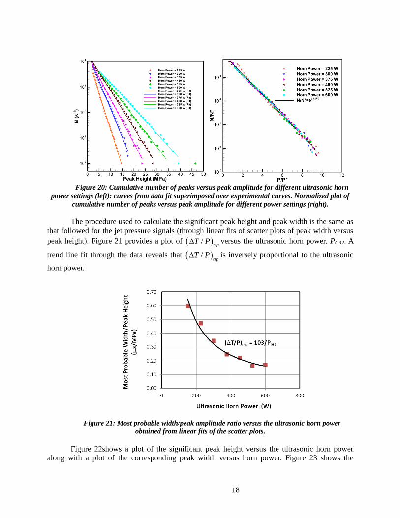
Figure 20 shows plots of the cumulative number of peaks, N, versus peak height and plots

of normalized cumulative number of peaks, N / *N , versus normalized peak height, P / *P , for

different ultrasonic horn power settings. Similar to the jet pressure measurements, the global

shapes of the N(P) experimental curves corresponding to different horn powers was found to be

well captured by the Weibull distribution function (Equation (6)). A curve fit shape parameter, k,

of 1 (2.54 for jets) results in the best least square fits to measured statistical data sets for all

ultrasonic horn power settings.

18

Figure 20: Cumulative number of peaks versus peak amplitude for different ultrasonic horn

power settings (left): curves from data fit superimposed over experimental curves. Normalized plot of

cumulative number of peaks versus peak amplitude for different power settings (right).

The procedure used to calculate the significant peak height and peak width is the same as

that followed for the jet pressure signals (through linear fits of scatter plots of peak width versus

peak height). Figure 21 provides a plot of /mp

T P versus the ultrasonic horn power, PG32. A

trend line fit through the data reveals that /mp

T P is inversely proportional to the ultrasonic

horn power.

Figure 21: Most probable width/peak amplitude ratio versus the ultrasonic horn power

obtained from linear fits of the scatter plots.

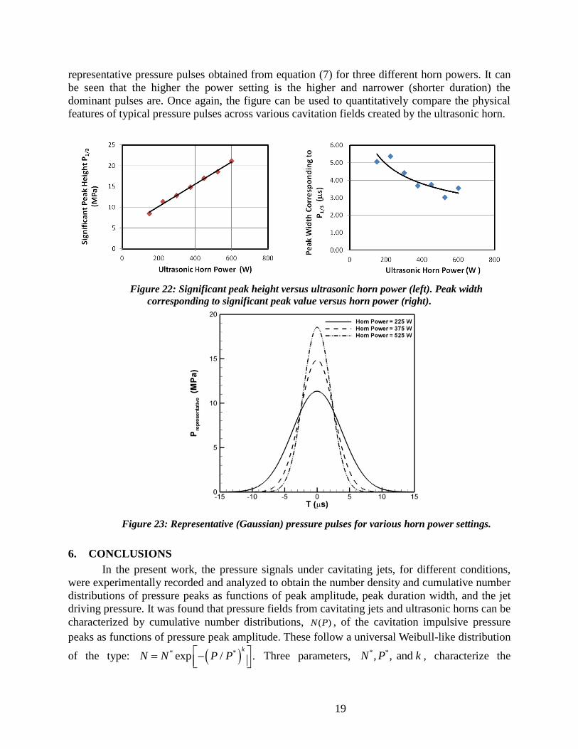
Figure 22shows a plot of the significant peak height versus the ultrasonic horn power

along with a plot of the corresponding peak width versus horn power. Figure 23 shows the

19

representative pressure pulses obtained from equation (7) for three different horn powers. It can

be seen that the higher the power setting is the higher and narrower (shorter duration) the

dominant pulses are. Once again, the figure can be used to quantitatively compare the physical

features of typical pressure pulses across various cavitation fields created by the ultrasonic horn.

Figure 22: Significant peak height versus ultrasonic horn power (left). Peak width

corresponding to significant peak value versus horn power (right).

Figure 23: Representative (Gaussian) pressure pulses for various horn power settings.

6. CONCLUSIONS

In the present work, the pressure signals under cavitating jets, for different conditions,

were experimentally recorded and analyzed to obtain the number density and cumulative number

distributions of pressure peaks as functions of peak amplitude, peak duration width, and the jet

driving pressure. It was found that pressure fields from cavitating jets and ultrasonic horns can be

characterized by cumulative number distributions, ( )N P , of the cavitation impulsive pressure

peaks as functions of pressure peak amplitude. These follow a universal Weibull-like distribution

of the type: * *exp / .k

N N P P

Three parameters,

* *, , and N P k , characterize the

20

cavitating flow field and are respectively a characteristic number of impulsive pressure peaks, a

characteristic amplitude of the impulsive pressure, and a distribution shape parameter.

Knowledge of these parameters can be a substitute to the need to know all statistical details of

the pressure field for the purpose of studying cavitation erosion. For both the cavitating jets and

the ultrasonic horn at different power setting a non-dimensional peak distribution of the shape kPN e . For the cavitating jets a value of k=2.54 was found, while for the ultrasonic horn k=1

was found to be more appropriate.

The most probable peak width to peak amplitude ratio was found to be inversely

proportional to the square of the jet pressure. This ratio is inversely proportional to the ultrasonic

horn power. A representative Gaussian pressure pulse can be constructed for each impulsive

pressure signal from both the jets and the ultrasonic horns, using a significant peak height

occurring in the pressure signal and the corresponding most probable peak width. From the

resulting representation of the cavitation field, it is clear that the dominant pressure pulses are

higher and narrower (shorter duration) as the jet pressure or the ultrasonic horn power increases.

This representation enables quantification and comparison of the impulsive pressure pulses,

which occur in different cavitation fields at various intensities of cavitation.

The mechanism resulting in higher and narrower peaks with increased cavitation intensity

(higher jet pressures or larger amplitude oscillations of the ultrasonic horn) may be understood

based on an insight into the physical characteristics of these flows. As the cavitation intensity

becomes higher, the cavitation bubbles experience greater pressure changes. For example for a

higher pressure jet the pressure changes involve a larger pressure drop across the nozzle, which

makes the bubble nuclei grow larger, and also a greater stagnation pressure near the jet impact

region, which makes the bubble collapse much stronger. These contribute to a higher peak as the

jet pressure increases. The same can be said as the amplitude of the pressure field oscillations

increases in the ultrasonic field.

Also as the cavitation intensity becomes higher both the jet velocity, which is

proportional to the square root of the driving pressure ( ~jetV p ), and the velocities in the

ultrasonic field, which are proportional to the amplitude of oscillation also increase. A faster

moving jet has two effects. It results in more number of bubbles pass by the impact region, and

results in a shorter duration of the bubble pulse for a given location of an erosion spot due to the

motion of the bubble.

Moreover, the correlation between the severity of cavitation and the magnitude of jet

pressure or power of the ultrasonic horn has been observed through erosion tests conducted over

several material sample under these test conditions [1, 27, 28, 29].

The pressure pulse analysis scheme developed in this work can be used in studies to

characterize the cavitation field intensity and build a database of various cavitation fields at

multiple scales. Well established understanding of the cavitation fields and proper

characterization of the cavitation intensity will enable better estimation of the expected cavitation

erosion progression.

21

7. ACKNOWLEDGMENTS

This work was conducted at DYNAFLOW as a part of erosion modeling effort supported by

the Office of Naval Research under contract N00014-11-C-0378, monitored by Dr. Ki-Han Kim.

This support is acknowledged with gratitude.

8. REFERENCES 1. Choi J-K., Jayaprakash A., Chahine G. L., Scaling of Cavitation Erosion Progression with

Cavitation Intensity and Cavitation Source, Wear 278–279, 53–61, 2012.

2. Pereira F., Avellan F., Dupont P., Prediction of Cavitation Erosion: An Energy Approach, Trans.

ASME, Journal of Fluids Engineering, 120 (4):719-727, 1998.

3. Knapp, R. T., Daily, J. W., and Hammitt, F. G., Cavitation, McGraw Hill Book Co., NY, 1970.

4. Hammitt F.G., Cavitation and Multiphase Flow Phenomena, McGraw-Hill International Book

Co., NY,1980.

5. Annual Book of ASTM Standards – Section 3 Material Test Methods and Analytical Procedures,

American Society for Testing and Materials (ASTM), Vol. 03.02, 2010.

6. Besant, W. H., Hydrostatics and hydrodynamics, Cambridge University Press, London, Art. 158,

1859.

7. Rayleigh, L., “On the Pressure Developed in a Liquid During the Collapse of a Spherical Cavity”,

Philosophical Magazine, series 4, 34, p. 94-98, 1917.

8. Mørch, K. A. 1979. “Dynamics of Cavitation Bubbles and Cavitating Liquids” , Treatise on

Materials Science and Technology Vol. 16: 309-355.

9. D'Agostino, L. and Brennen, C.E., "On the Acoustical Dynamics of Bubble Clouds”, ASME

Cavitation and Polyphase Flow Forum, Houston, 72-76, 1983.

10. Chahine, G. L., "Cavitation Cloud Theory," Proceedings, 14th Symposium on Naval

Hydrodynamics, Ann Arbor, Michigan, National Academy Press, pp. 165-194, Washington, D.C.,

1983.

11. Reisman, G. E., Wang, Y.-C. and Brennen, C. E., “Observations of shock waves in cloud

cavitation,” J. of Fluid Mechanics, 1998. 355, p. 255-283.

12. G. L. Chahine, “Pressures Generated by a Bubble Cloud Collapse,” Chemical Engineering

Communications, July 1984, Vol. 28, No. 4-6, pp. 355-364.

13. Chahine, G. L. and Duraiswami, R., "Dynamical Interactions in a Bubble Cloud", Trans. of the

ASME, Journal of Fluids Engineering, Vol.114, p.680, 1992.

14. Tomita, Y., et al., “Peeling off effect and damage pit formation by ultrasonic cavitation”, The

International Conference on Hydraulic Machinery and Equipments. 2008: Timisoara, Romania. p.

19-24.

15. Haosheng, C. and L. Shihan, “Inelastic damages by stress wave on steel surface at the incubation

stage of vibration cavitation erosion”, Wear, 2009. 266(1-2): p. 69-75.

16. Haosheng, C., et al., “Damages on steel surface at the incubation stage of the vibration cavitation

erosion in water”, Wear, 2008. 265(5-6): p. 692-698.

17. Sato, K., Sugimoto, Y., Ohjimi, S., “Pressure-Wave Formation and Collapses of Cavitation

Clouds Impinging on Solid Wall in a submerged Water Jet”, Proceedings of the 7th International

Symposium on Cavitation (CAV 2009), August 17-22, 2009, Ann Arbor, Michigan, USA.

18. Hulti, E. A. F. and Nedeljkovic, M. S., “Frequency in shedding/discharging cavitation clouds

determined by visualization of a submerged cavitating jet,” Trans. ASME, J. of Fluids

Engineering, 2008. 130, 021304, p. 1-8.

19. Soyama, H., Yamauchi, Y., Adachi, Y., Shindo, T., Oba, R. and Sato, K., “High-speed cavitation-

cloud observations around high-speed submerged water jets,” Proc. 2nd

International Symposium

on Cavitation, 1994. p. 225-230.

22

20. Vijay, M. M., Zou, C., and Tavoularis, S., “A study of the characteristics of cavitating water jets

by photography and erosion,” Proc. of Tenth International Conference, Jet Cutting Technology,

1990. p. 37-67.

21. Yamaguchi, A. and Shimizu, S., “Erosion due to impingement of cavitating jet,” Trans. ASME, J.

of Fluids Engineering, 1987. 109: p. 442-447.

22. Chahine G. L., and Johnson V. E. Jr., "Mechanics and Applications of Self-Resonating Cavitating

Jets", International Symposium on Jets and Cavities, ASME, WAM, Miami, FL, Nov. 1985.

23. G. L. Chahine, P. Courbière, “Noise and Erosion of Self-Resonating Cavitating Jets”, Journal of

Fluids Engineering 109 (1987) 429-435.

24. Jayaprakash, A., Hsiao, C.-T., Chahine, G. L., “Numerical and Experimental Study of the

Interaction of a Spark-Generated Bubble and a Vertical Wall”, Trans. ASME, Journal of Fluid

Engineering, Volume 134, 031301, March 2012.

25. Denny, M.W., “Biology and the Mechanics of Wave-swept Shores”, Princeton University Press,

1988, ISBN 0691084874.

26. Munk, W. H., “Proposed uniform procedure for observing waves and interpreting instrument

records” La Jolla, California: Wave Project at the Scripps Institute of Oceanography, 1944.

27. Franc, J-P., Riondet, M., Karimi, A., and Chahine, G. L., “Material and velocity effects on

cavitation erosion pitting”, Wear 274–278, 248–259, 2012.

28. Jayaprakash, A., Choi, J-K., Chahine, G. L., Martin, F., Donnelly, M., Franc, J-P., and Karimi, A.,

“Scaling study of cavitation pitting from cavitating jets and ultrasonic horns", Wear 296, 619-629,

2012.

29. Franc, J-P., Riondet, M., Karimi, A., and Chahine, G. L., “Impact Load Measurements in an

Erosive Cavitating Flow”, Trans. of the ASME, Journal of Fluids Engineering, Vol. 133, 2011.