Chapter Six Firms and Production. © 2007 Pearson Addison-Wesley. All rights reserved.6–2 Firms and Production In this chapter, we examine six main topics

Chapter Six

Firms and Production

© 2007 Pearson Addison-Wesley. All rights reserved. 6–2

Firms and Production

• In this chapter, we examine six main topics.– The ownership and management of firms– Production– Short-run production– Long-run production– Return to scale – Productivity and technical change


The Ownership and Management of Firms

• firm– an organization that converts inputs such

as labor, materials, energy, and capital into outputs, the goods and services that it sells


The ownership of Firms• In most countries, for-profit firms have one of

three legal forms: sole proprietorship, partnerships, and corporations.– Sole proprietorships are firms owned and run

by a single individual.

– Partnerships are businesses jointly owned and controlled by two or more people. The owners operate under a partnership agreement.

– Corporations are owned by shareholders in proportion to the numbers of shares of stock they hold. The shareholders elect a board of directors who run the firm.


• Corporations differ from the other two forms of ownership in terms of personal liability for the debts of the firm.

• Corporations have limited liability: The personal assets of the corporate owners cannot be taken to pay a corporation’s debts if it goes into bankruptcy.

The ownership of Firms


• limited liability– condition whereby the personal assets of

the owners of the corporation cannot be taken to pay a corporation’s debts if it goes into bankruptcy

• Sole proprietors and partnerships have unlimited liability － that is, even their personal assets can be taken to pay the firm’s debts.

The ownership of Firms


台灣廠商的組織型式

組織別 80年 85年 90年總計 100 100 100

民營公司 99.873 99.914 99.358

公司組織 29.421 38.286 37.254

獨資與合夥 69.674 61.15 61.492

其他組織 0.778 0.477 0.612

公營公司 0.127 0.086 0.642

公司組織 0.0134 0.0112 0.2147

非公司組織 0.1137 0.0752 0.4274

單位：以百分比計算

資料來源：行政院主計處 90 年工商普查資料


The Management of Firms

• In a small firm, the owner usually manages the firm’s operations.

• In larger firms, typically corporations and larger partnerships, a manager or team of managers usually runs the company.


What Owners Want

• Economists usually assume that a firm’s owners try to maximize profit.

• profit ( )– the difference between revenues, R, and

costs, C: ＝ R － C

• To maximize profits, a firm must produce as efficiently as possible as we will consider in this chapter.


• efficient production or technological efficiency– situation in which the current level of output

cannot be produced with fewer inputs, given existing knowledge about technology and the organization of production

• If the firm does not produce efficiently, it cannot be profit maximizing － so efficient production is a necessary condition for profit maximization.

What Owners Want


Production

• A firm uses a technology or production process to transform inputs or factors of production into outputs.– Capital (K)– Labor (L)– Materials (M)


• The various ways inputs can be transformed into output are summarized in the production function: the relationship between the quantities of inputs used and the maximum quantity of output that can be produced, given current knowledge about technology and organization. The production function for a firm that uses only labor and capital is

q ＝ f (L, K), (6.1)

where q units of output (wrapped candy bars) are produced using L units of labor services (days of work by relatively unskilled assembly-line workers) and K units of capital (the number of conveyor belts).

Production Functions


• The production function shows only the maximum amount of output that can be produced from given levels of labor and capital, because the production function includes only efficient production processes.

Production Functions


Time and the Variability of Inputs

• short run– a period of time so brief that at least one

factor of production cannot be varied practically

• fixed input– a factor of production that cannot be varied

practically in the short run


• variable input – a factor of production whose quantity can

be changed readily by the firm during the relevant time period

• long run– a lengthy enough period of time that all

inputs can be varied

Time and the Variability of Inputs


Short-Run Production: One Variable and One Fixed Input

• In the short run, we assume that capital is fixed input and labor is a variable input.

• In the short run, the firm’s production function is

(6.2)

where q is output, L is workers, and is the fixed number of units of capital.

( , ) q f L K

K


Total Product

• The exact relationship between output or total product and labor can be illustrated by using a particular function, Equation 6.2, a table, or a figure.


Table 6.1 Total Product, Marginal Product, and Average Product of Labor with Fixed Capital


Marginal Product of Labor

• marginal product of labor (MPL)

– the change in total output, , resulting from using an extra unit of labor, , holding other factors constant:

q

/LMP q L ＝

L


Average Product of Labor

• average product of labor (APL)

– the ratio of output, q, to the number of workers, L, used to produce that output:

APL = q/L


Total Product of Labor

• The amount of output (or total product) that can be produced by a given amount of labor


Figure 6.1 Production Relationships with Variable Labor

B

A

C

11640L, Workers per day

Marginal product, MPL

Average product, APL

110

90

56

(a)

b

a

c

11640

L, Workers per day

20

15

(b)


Effect of Extra Labor

• In most production processes, the average product of labor first rises and then falls as labor increases.


Relationship of the Product Curves

• The average product of labor curve slopes upward where the marginal product of labor curve is above it and slopes downward where the marginal product curve is below it.


• The average product of labor for L workers equals the slope of a straight line from the origin to a point on the total product of labor curve for L workers in panel a.




• The slope of the total product curve at a given point, , equals the marginal product of labor.

/q L


Law of Diminishing Marginal Returns

• The law of diminishing marginal returns (or diminishing marginal product) holds that, if a firm keeps increasing an input, holding all other inputs and technology constant, the corresponding increases in output will become smaller eventually.


• Where there are “diminishing marginal returns,” the MPL curve is falling.

• Within “diminishing returns,” extra labor causes output to fall.



• Thus saying that there are diminishing returns is much stronger than saying that there are diminishing marginal returns. We often observe firms producing where there are diminishing marginal returns to labor, but we rarely see firms operating where there are diminishing total returns.



• A second common misinterpretation of this law is to claim that marginal products must fall as we increase an input without requiring that technology and other inputs stay constant.



Long-Run Production: Two Variable Inputs

• In the long run, however, both inputs are variable. With both factors variable, a firm can usually produce a given level of output by using a great deal of labor and very little capital, a great deal of capital and very little labor, or moderate amounts of both.


Isoquants

• isoquant– a curve that shows the efficient

combinations of labor and capital that can produce a single (iso) level of output (quantity)

• We can use these isoquants to illustrate what happens in the short run when capital is fixed and only labor varies.


Table 6.2 Output Produced with Two Variable Inputs


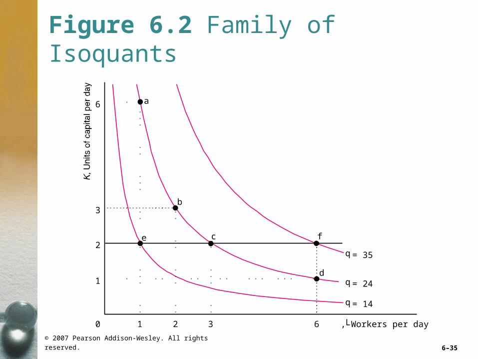
Properties of Isoquants

• First, the farther an isoquant is from the origin, the greater the level of output.

• Second, isoquants do not cross.

• Third, isoquants slope downward.


Figure 6.2 Family of Isoquants

e

b

a

d

fc

63210 L, Workers per day

6

3

2

1

q = 14

q = 24

q = 35


Shape of Isoquants

• The curvature of an isoquant shows how readily a firm can substitute one input for another.

• If the inputs are perfect substitutes, each isoquant is a straight line.

• The production function is

q = x + y


• Sometimes it is impossible to substitute one input for the other: Inputs must be used in fixed proportion.

• Such a production function is called a fixed-proportions production function.

Shape of Isoquants


Figure 6.3 Substitutability of Inputs

(a)

x, Maine potatoes per day

q = 3q = 2q = 1

(b)

Cereal per day

q = 3

q = 2

q = 1

45 line


Figure 6.3 Substitutability of Inputs (cont’d)

q = 1

(c)

L, Labor per unit of time


Substituting Inputs

• The slope of an isoquant shows the ability of a firm to replace one input with another while holding output constant.

• The slope of an isoquant is called the marginal rate of technological substitution (MRTS):

change in capital

change in labor

K

MRTSL


• marginal rate of technical substitution– the number of extra units of one input

needed to replace one unit of another input that enables a firm to keep the amount of output it produces constant

Substituting Inputs


Figure 6.4 How the Marginal Rate of Technical Substitution Varies Along an Isoquant

L, Workers per day

45

7

10

16a

b

cd

eq = 10

∆K = –6

∆L = 1

0 1

1

1

1

2 3

–3

–2–1

4 5 6 7 8 9 10

MRTS in a Printing and Publishing U.S. Firm


Substitutability of Inputs Varies Along an Isoquant

• The marginal rate of technical substitution varies along a curved isoquant.

• This decline in the MRTS (in absolute value) along an isoquant as the firm increases labor illustrates diminishing marginal rates of technical substitution.


Substitutability of Inputs and Marginal Products

• The marginal rate of technical substitution—the degree to which inputs can be substituted for each other—equals the ratio of the marginal products of labor to the marginal product of capital.


Substitutability of Inputs and Marginal Products

• To keep output constant, , this fall in output from reducing capital must exactly equal the increase in output from increasing labor:

rearranging these terms, we find that

(6.3)

0q

( ) ( ) 0L KMP L MP K

L

K

MP KMRTS

MP L


Returns to Scale

• How much output changes if a firm increases all its inputs proportionately? The answer helps a firm determine its scale or size in the long run.


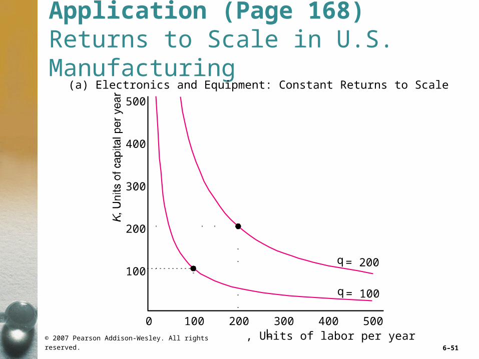
Constant, Increasing, and Decreasing Returns to Scale

• constant returns to scale (CRS)– property of a production function whereby

when all inputs are increased by a certain percentage, output increases by that same percentage



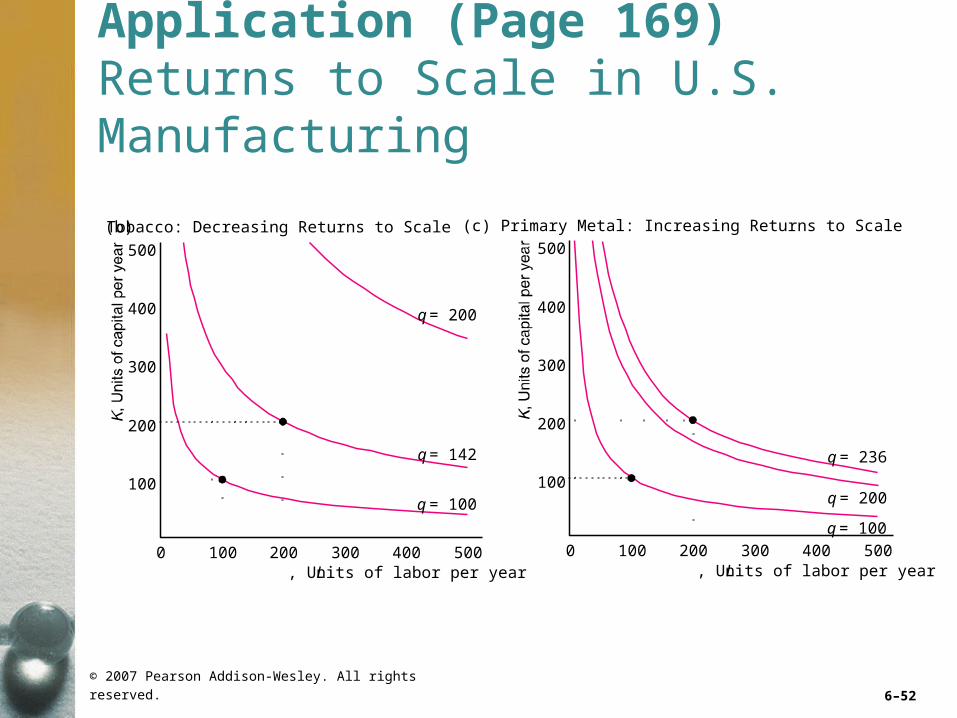
• increasing returns to scale (IRS)– property of a production function whereby

when output rises more than in proportion to an equal increase in all inputs

• A technology exhibits increasing returns to scale if doubling inputs more than doubles the output: (2 ,2 ) 2 ( , )f L K f L K



• decreasing returns to scale (DRS)– property of a production function whereby

output increase less than in proportion to an equal percentage increase in all inputs

• A technology exhibits decreasing returns to scale if doubling inputs causes output to rise less than in proportion: (2 ,2 ) 2 ( , )f L K f L K


Application (Page 168) Returns to Scale in U.S. Manufacturing



L, Units of labor per year

300

400

500

100

200

q = 100

q = 200

0 100 200 300 400 500

(a) Electronics and Equipment: Constant Returns to Scale




300

400

500

100

200

q = 100

q = 200

q = 236

0 100 200 300 400 500

(c) Primary Metal: Increasing Returns to Scale


300

400

500

100

200

q = 100

q = 142

q = 200

0 100 200 300 400 500

(b) Tobacco: Decreasing Returns to Scale


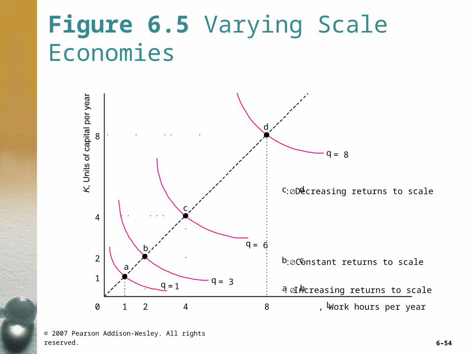
Varying Returns to Scale

• Many production functions have increasing returns to scale for small amounts of output, constant returns for moderate amounts of output, and decreasing returns for large amounts of output.

• The spacing of the isoquants reflects the returns to scale.


Figure 6.5 Varying Scale Economies

41 2

a

b

d

c

a b: Increasing returns to scale

b c: Constant returns to scale

c d: Decreasing returns to scale

8 L, Work hours per year

4

2

1

0

8

q = 8

q = 6

q = 3q = 1


Productivity and Technical Change

• Relative Productivity

– We can measure the relative productivity of a firm by expressing the firm’s actual output, q, as a percentage of the output that the most productive firm in the industry could have produced, q*, from the same amount of inputs: 100q/q*.


Innovations

• technical progress– an advance in knowledge that allows more

output to be produced with the same level of inputs


Technical Progress

• A technological innovation changes the production process.

• Last year a firm produced

units of output using L units of labor services and K units of capital service.

1 ( , )q f L K


Technical Progress

• This year’s production function differs from last year’s, so the firm produces 10% more output with the same inputs:

• This firm has experienced neutral technical change, in which it can produce more output using the same ratio of inputs.

2 1.1 ( , )q f L K


• Nonneutral technical changes are innovations that alter the proportion in which inputs are used.

Technical Progress


Organizational Change

• Organizational changes may also alter the production function and increase the amount of output produced by a given amount of inputs.


Table 6.3 Annual Percentage Rates


Documents

Chapter Six Firms and Production. © 2007 Pearson Addison-Wesley. All rights reserved.6–2 Firms and Production In this chapter, we examine six main topics