Embed Size (px)
Citation preview
© 2008 Pearson Addison Wesley. All rights reserved
Chapter Six
Firms and Production
Firms and Production
• In this chapter, we examine six topics
- The Ownership and Management of Firms
- Production
- Short-Run Production
- Long-Run Production
- Returns to Scale
- Productivity and Technical Change
© 2008 Pearson Addison Wesley. All rights reserved. 6-2
The Ownership and Management of Firms
• Firm
–an organization that converts inputs such as labor, materials, energy, and capital into outputs, the goods and services that it sells.
© 2008 Pearson Addison Wesley. All rights reserved. 6-3
The Ownership and Management of Firms
• In most countries, for-profit firms have one of three legal forms:– Sole proprietorships are firms owned and run by a single individual.
– Partnerships are businesses jointly owned and controlled by two or more people. The owners operate under a partnership agreement.
– Corporations are owned by shareholders in proportion to the numbers of shares of stock they hold. The shareholders elect a board of directors who run the firm.
© 2008 Pearson Addison Wesley. All rights reserved. 6-4
The Ownership of Firms
• Corporations differ from the other two forms of ownership in terms of personal liability for the debts of the firm.
• Corporations have limited liability: The personal assets of the corporate owners cannot be taken to pay a corporation’s debts if it goes into bankruptcy.
© 2008 Pearson Addison Wesley. All rights reserved. 6-5
The Ownership of Firms
• Limited Liability–condition whereby the personal assets of the owners of the corporation cannot be taken to pay a corporation’s debts if it goes into bankruptcy
• Sole proprietors and partnerships have unlimited liability - that is, even their personal assets can be taken to pay the firm’s debts.
© 2008 Pearson Addison Wesley. All rights reserved. 6-6
The Management of Firms
• In a small firm, the owner usually manages the firm’s operations.
• In larger firms, typically corporations and larger partnerships, a manager or team of managers usually runs the company.
© 2008 Pearson Addison Wesley. All rights reserved. 6-7
What Owners Want
• Economists usually assume that a firm’s owners try to maximize profit.
• profit ( )–the difference between revenues, R, and costs, C: = R - C
• To maximize profits, a firm must produce as efficiently as possible as we will consider in this chapter.
© 2008 Pearson Addison Wesley. All rights reserved. 6-8
What Owners Want
• Efficient Production or Technological Efficiency–situation in which the current level of output cannot be produced with fewer inputs, given existing knowledge about technology and the organization of production
• If the firm does not produce efficiently, it cannot be profit maximizing - so efficient production is a necessary condition for profit maximization.
© 2008 Pearson Addison Wesley. All rights reserved. 6-9
Production
• A firm uses a technology or production process to transform inputs or factors of production into outputs.
–Capital (K)–Labor (L)–Materials (M)
© 2008 Pearson Addison Wesley. All rights reserved. 6-10
Production Functions
• The various ways inputs can be transformed into output are summarized in the production function: the relationship between the quantities of inputs used and the maximum quantity of output that can be produced, given current knowledge about technology and organization. The production function for a firm that uses only labor (L) and capital (K) is
q = f (L, K), (6.2)
where q units of output are produced. © 2008 Pearson Addison Wesley. All rights reserved. 6-11
Production Functions
• The production function shows only the maximum amount of output that can be produced from given levels of labor and capital, because the production function includes only efficient production processes.
© 2008 Pearson Addison Wesley. All rights reserved. 6-12
Time and the Variability of Inputs
• Short Run–a period of time so brief that at least one factor of production cannot be varied practically
• Fixed Input–a factor of production that cannot be varied practically in the short run
© 2008 Pearson Addison Wesley. All rights reserved. 6-13
Time and the Variability of Inputs
• Variable Input –a factor of production whose quantity can be changed readily by the firm during the relevant time period
• Long Run–a lengthy enough period of time that all inputs can be varied
© 2008 Pearson Addison Wesley. All rights reserved. 6-14
Short-Run Production: One Variable and One Fixed Input
• In the short run, we assume that capital is fixed input and labor is a variable input.
• In the short run, the firm’s production function is
(6.3)
where q is output, L is workers, and is the fixed number of units of capital.
© 2008 Pearson Addison Wesley. All rights reserved. 6-15
K
Total Product of Labor
• The exact relationship between output or total product and labor can be illustrated by using a particular function, Equation 6.3, or a figure, Figure 6.1.
© 2008 Pearson Addison Wesley. All rights reserved. 6-16
© 2008 Pearson Addison Wesley. All rights reserved. 6-17
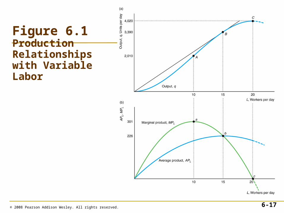
Figure 6.1Production Relationships with Variable Labor
Marginal Product of Labor
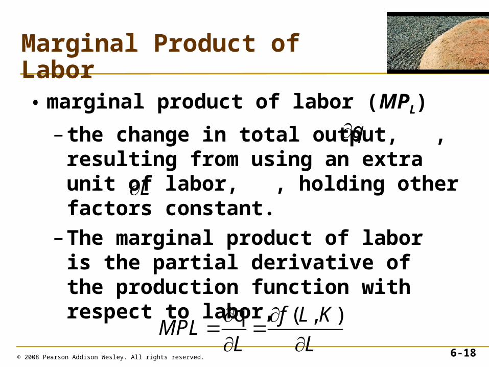
• marginal product of labor (MPL)
–the change in total output, , resulting from using an extra unit of labor, , holding other factors constant.
–The marginal product of labor is the partial derivative of the production function with respect to labor,
© 2008 Pearson Addison Wesley. All rights reserved. 6-18
q ( , )
f L K
MPLL L
q
L
Average Product of Labor
• average product of labor (APL)
–the ratio of output, q, to the number of workers, L, used to produce that output:
APL = q/L
© 2008 Pearson Addison Wesley. All rights reserved. 6-19
Relationship of the Product Curves
• The average product of labor curve slopes upward where the marginal product of labor curve is above it and slopes downward where the marginal product curve is below it.
© 2008 Pearson Addison Wesley. All rights reserved. 6-20
Law of Diminishing Marginal Returns
• The law of diminishing marginal returns (or diminishing marginal product) holds that, if a firm keeps increasing an input, holding all other inputs and technology constant, the corresponding increases in output will become smaller eventually.
© 2008 Pearson Addison Wesley. All rights reserved. 6-21
Law of Diminishing Marginal Returns
• Where there are “diminishing marginal returns,” the MPL curve is falling.
• Within “diminishing returns,” extra labor causes output to fall.
• Thus saying that there are diminishing returns is much stronger than saying that there are diminishing marginal returns.
© 2008 Pearson Addison Wesley. All rights reserved. 6-22
Long-Run Production: Two Variable Inputs
• In the long run, however, both inputs are variable. With both factors variable, a firm can usually produce a given level of output by using a great deal of labor and very little capital, a great deal of capital and very little labor, or moderate amounts of both.
© 2008 Pearson Addison Wesley. All rights reserved. 6-23
© 2008 Pearson Addison Wesley. All rights reserved. 6-24
Equation 6.4
Isoquants
• isoquant
–a curve that shows the efficient combinations of labor and capital that can produce a single (iso) level of output (quantity)
• We can use these isoquants to illustrate what happens in the short run when capital is fixed and only labor varies.
© 2008 Pearson Addison Wesley. All rights reserved. 6-25

© 2008 Pearson Addison Wesley. All rights reserved. 6-26
Equation 6.5
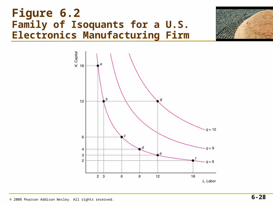
Properties of Isoquants
• First, the farther an isoquant is from the origin, the greater the level of output.
• Second, isoquants do not cross.
• Third, isoquants slope downward.
© 2008 Pearson Addison Wesley. All rights reserved. 6-27
© 2008 Pearson Addison Wesley. All rights reserved. 6-28
Figure 6.2Family of Isoquants for a U.S. Electronics Manufacturing Firm
Shape of Isoquants
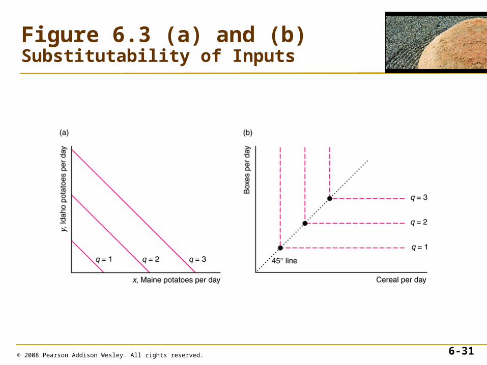
• The curvature of an isoquant shows how readily a firm can substitute one input for another.
• If the inputs are perfect substitutes, each isoquant is a straight line.
• The production function is
q = x + y
© 2008 Pearson Addison Wesley. All rights reserved. 6-29
Shape of Isoquants
• Sometimes it is impossible to substitute one input for the other: Inputs must be used in fixed proportion.
• Such a production function is called a fixed-proportions production function.
• The fixed-proportions production function is given by:
q = min(g, b).
© 2008 Pearson Addison Wesley. All rights reserved. 6-30
© 2008 Pearson Addison Wesley. All rights reserved. 6-31
Figure 6.3 (a) and (b)Substitutability of Inputs
© 2008 Pearson Addison Wesley. All rights reserved. 6-32
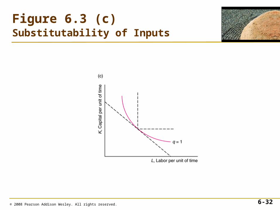
Figure 6.3 (c)Substitutability of Inputs
Substituting Inputs
• The slope of an isoquant shows the ability of a firm to replace one input with another while holding output constant.
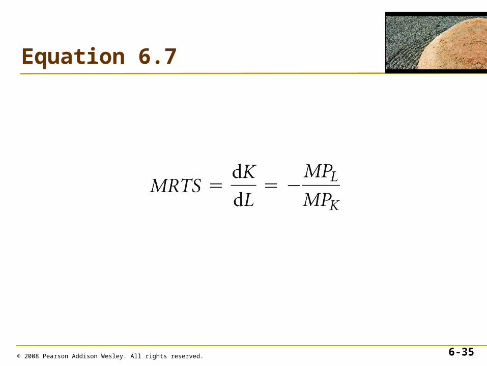
• The slope of an isoquant is called the marginal rate of technological substitution (MRTS).
© 2008 Pearson Addison Wesley. All rights reserved. 6-33
© 2008 Pearson Addison Wesley. All rights reserved. 6-34
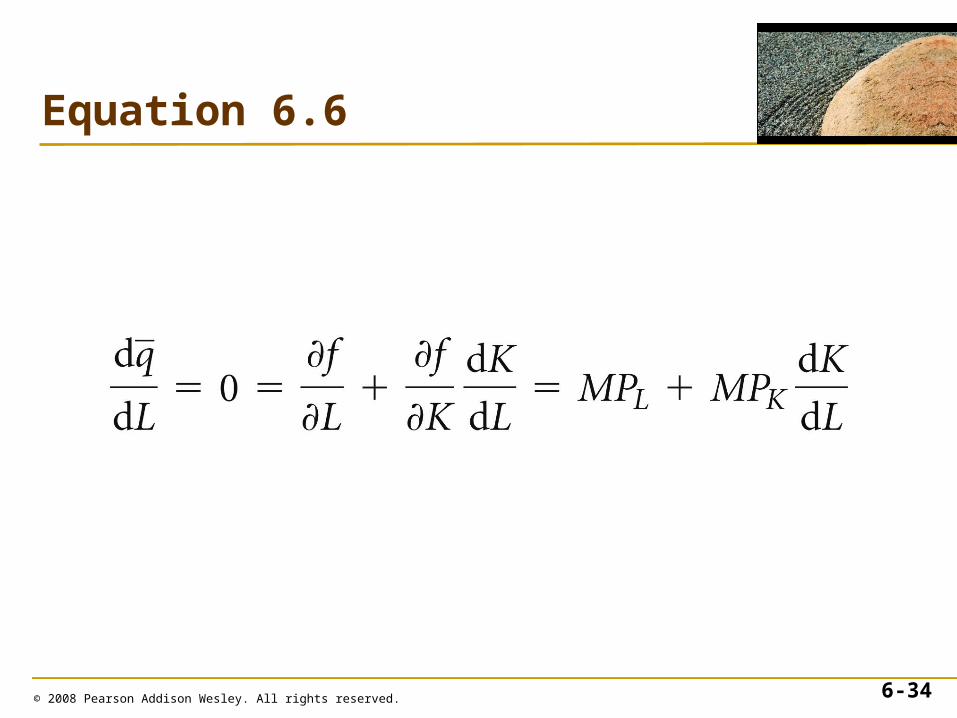
Equation 6.6
© 2008 Pearson Addison Wesley. All rights reserved. 6-35
Equation 6.7
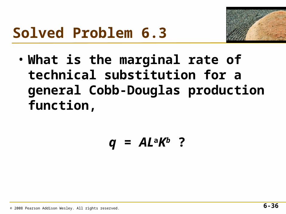
Solved Problem 6.3
• What is the marginal rate of technical substitution for a general Cobb-Douglas production function,
q = ALaKb ?
© 2008 Pearson Addison Wesley. All rights reserved. 6-36
© 2008 Pearson Addison Wesley. All rights reserved. 6-37
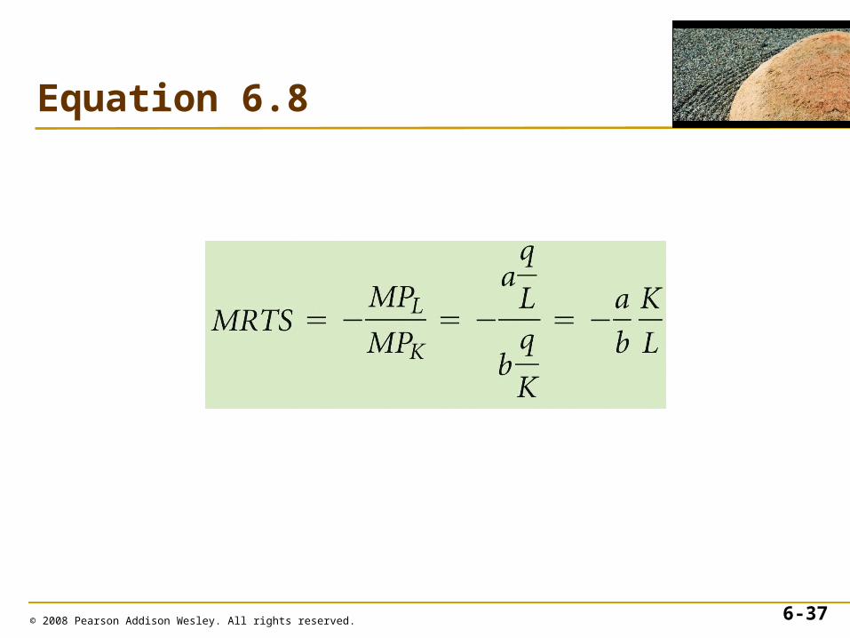
Equation 6.8
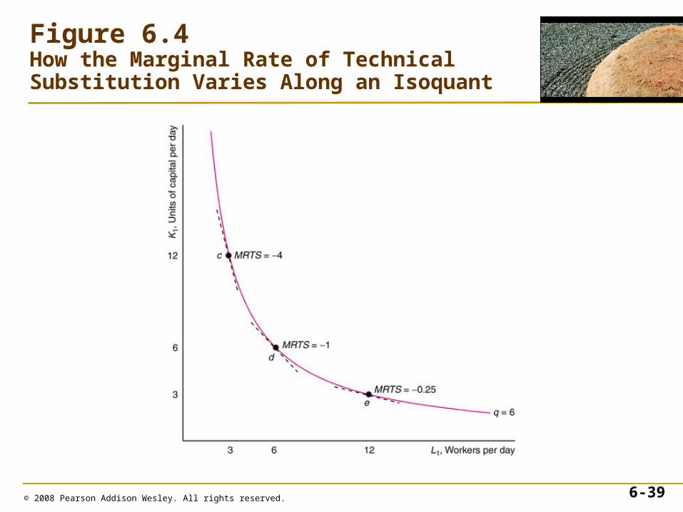
Diminishing Marginal Rates of Technical Substitution
• The marginal rate of technical substitution varies along a curved isoquant.
• This decline in the MRTS (in absolute value) along an isoquant as the firm increases labor illustrates diminishing marginal rates of technical substitution.
© 2008 Pearson Addison Wesley. All rights reserved. 6-38
© 2008 Pearson Addison Wesley. All rights reserved. 6-39
Figure 6.4How the Marginal Rate of Technical Substitution Varies Along an Isoquant
The Elasticity of Substitution
• The elasticity of substitution, , is the percentage change in the capital-labor ratio divided by the percentage change in the MRTS.
• This measure reflects the ease with which a firm can substitute capital for labor.
© 2008 Pearson Addison Wesley. All rights reserved. 6-40
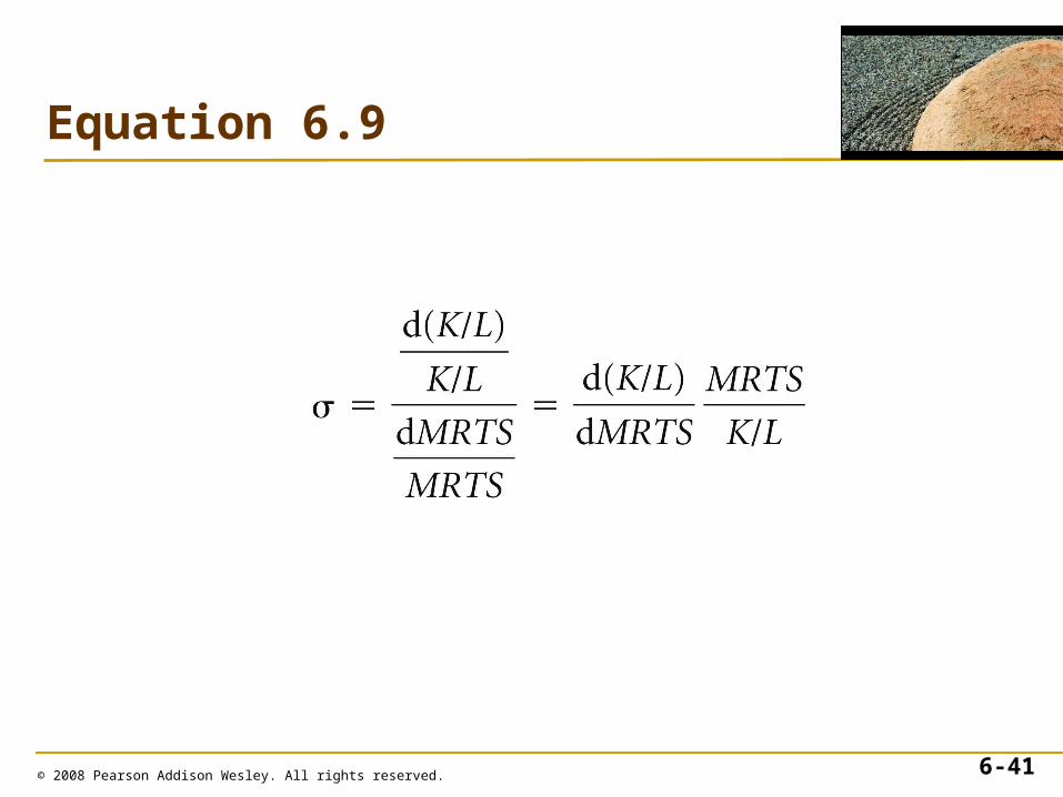
© 2008 Pearson Addison Wesley. All rights reserved. 6-41
Equation 6.9
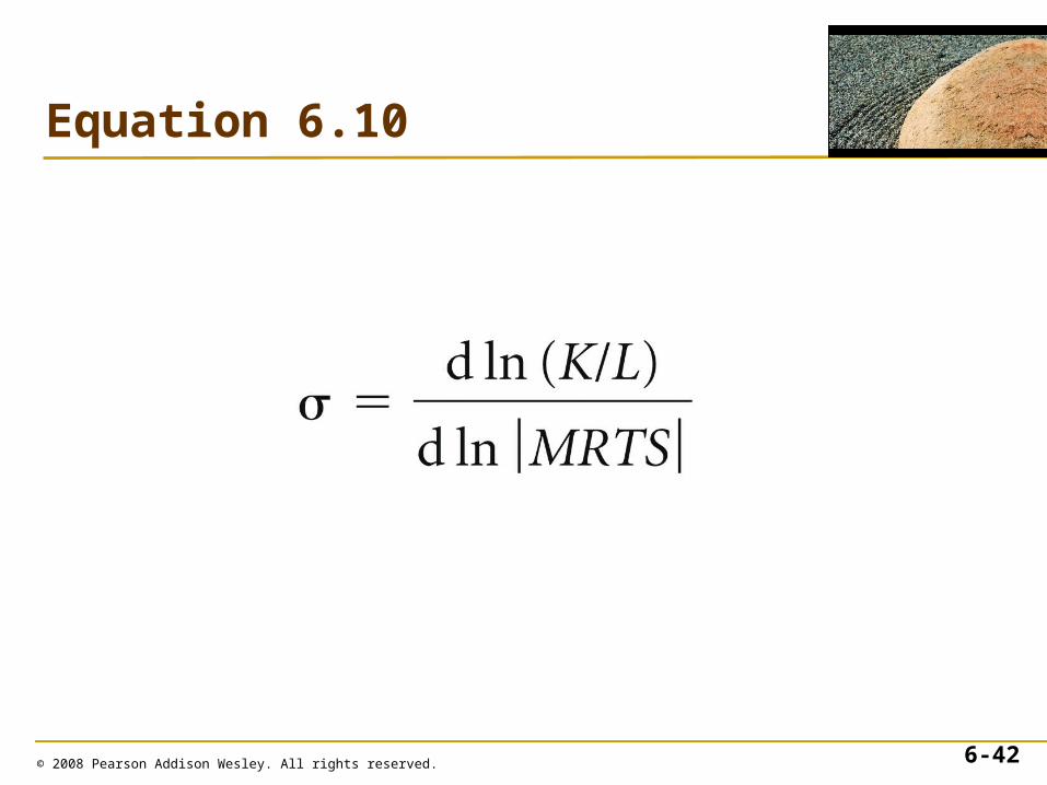
© 2008 Pearson Addison Wesley. All rights reserved. 6-42
Equation 6.10
The Elasticity of Substitution
• Constant Elasticity of Substitution Production
- In general, the elasticity of substitution varies along an isoquant. An exception is the constant elasticity of substitution (CES) production function.
© 2008 Pearson Addison Wesley. All rights reserved. 6-43

© 2008 Pearson Addison Wesley. All rights reserved. 6-44
Equation 6.11
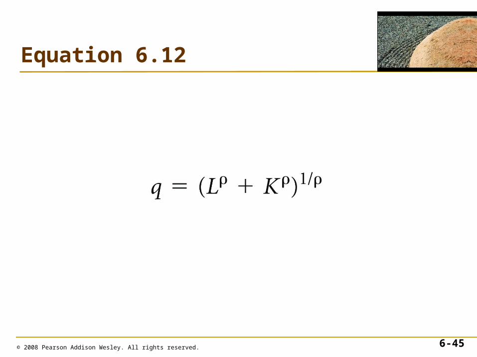
© 2008 Pearson Addison Wesley. All rights reserved. 6-45
Equation 6.12
© 2008 Pearson Addison Wesley. All rights reserved. 6-46
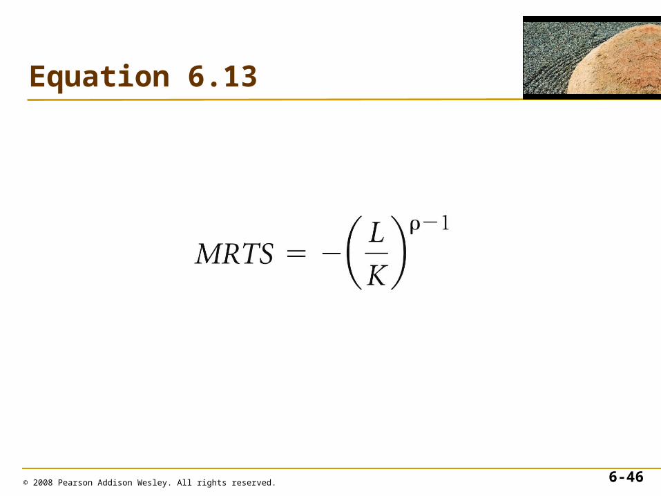
Equation 6.13

© 2008 Pearson Addison Wesley. All rights reserved. 6-47
Equation 6.14
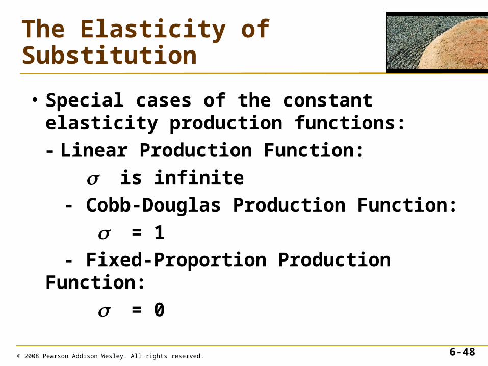
The Elasticity of Substitution
• Special cases of the constant elasticity production functions:
- Linear Production Function:
is infinite
- Cobb-Douglas Production Function:
= 1
- Fixed-Proportion Production Function:
= 0
© 2008 Pearson Addison Wesley. All rights reserved. 6-48
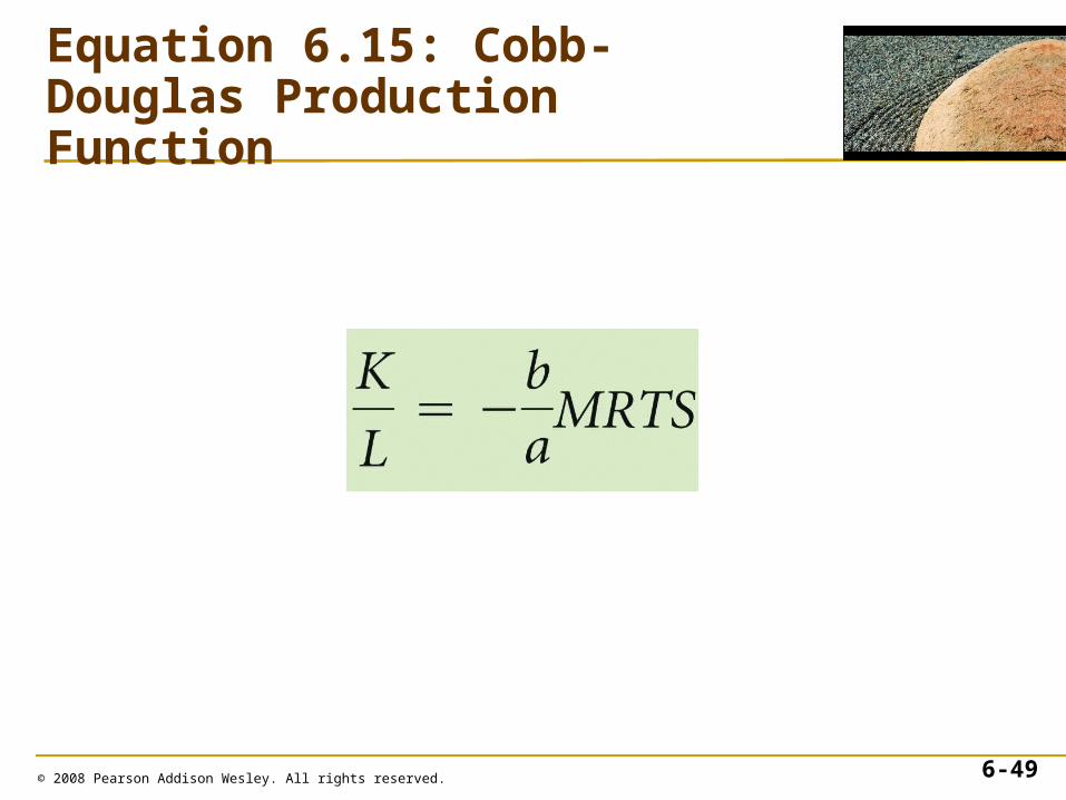
© 2008 Pearson Addison Wesley. All rights reserved. 6-49
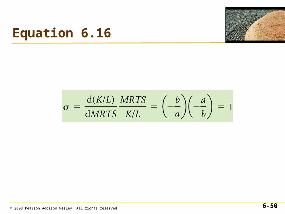
Equation 6.15: Cobb-Douglas Production Function
© 2008 Pearson Addison Wesley. All rights reserved. 6-50
Equation 6.16
Returns to Scale
• How much output changes if a firm increases all its inputs proportionately? The answer helps a firm determine its scale or size in the long run.
© 2008 Pearson Addison Wesley. All rights reserved. 6-51
Constant, Increasing, and Decreasing Returns to Scale
• constant returns to scale (CRS)
–property of a production function whereby when all inputs are increased by a certain percentage, output increases by that same percentage
© 2008 Pearson Addison Wesley. All rights reserved. 6-52
Constant, Increasing, and Decreasing Returns to Scale
• increasing returns to scale (IRS)–property of a production function whereby when output rises more than in proportion to an equal increase in all inputs
• A technology exhibits increasing returns to scale if doubling inputs more than doubles the output:
f(2L, 2K) > 2f(L, K)
© 2008 Pearson Addison Wesley. All rights reserved. 6-53
Constant, Increasing, and Decreasing Returns to Scale
• decreasing returns to scale (DRS)–property of a production function whereby output increase less than in proportion to an equal percentage increase in all inputs
• A technology exhibits decreasing returns to scale if doubling inputs causes output to rise less than in proportion: f(2L, 2K) < 2f(L, K)
© 2008 Pearson Addison Wesley. All rights reserved. 6-54
© 2008 Pearson Addison Wesley. All rights reserved. 6-55
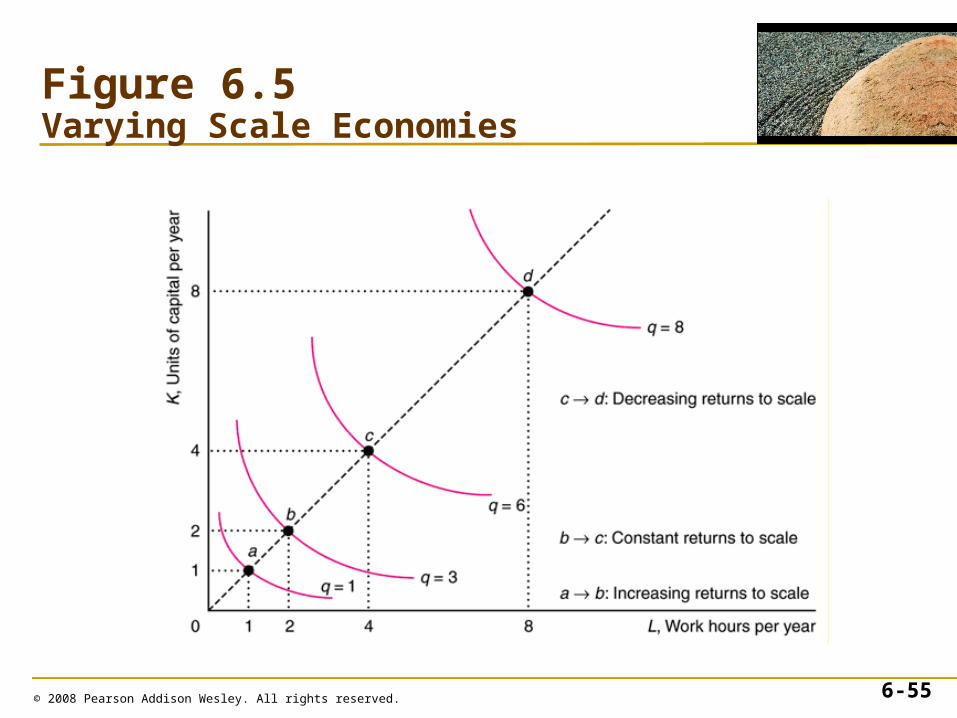
Figure 6.5Varying Scale Economies
Varying Returns to Scale
• Many production functions have increasing returns to scale for small amounts of output, constant returns for moderate amounts of output, and decreasing returns for large amounts of output.
• The spacing of the isoquants reflects the returns to scale.
© 2008 Pearson Addison Wesley. All rights reserved. 6-56
Productivity and Technical Change
• Relative Productivity–We can measure the relative productivity of a firm by expressing the firm’s actual output, q, as a percentage of the output that the most productive firm in the industry could have produced, q*, from the same amount of inputs: 100q/q*.
© 2008 Pearson Addison Wesley. All rights reserved. 6-57
Innovations
• Technical Progress–an advance in knowledge that allows more output to be produced with the same level of inputs
• Neutral Technical Progress
- The firm can produce more output using the same ratio of inputs.
q = A(t)f(L, K)© 2008 Pearson Addison Wesley. All rights reserved. 6-58
© 2008 Pearson Addison Wesley. All rights reserved. 6-59
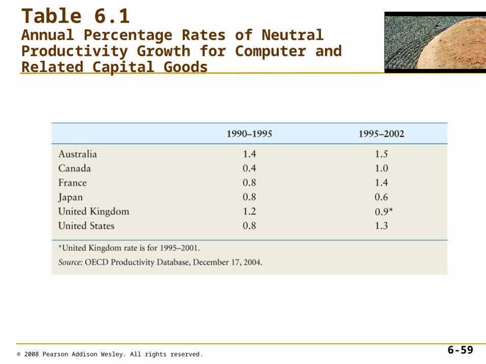
Table 6.1Annual Percentage Rates of Neutral Productivity Growth for Computer and Related Capital Goods
Innovations
• Nonneutral technical changes are innovations that alter the proportion in which inputs are used.
• Labor saving innovation: The ratio of labor to the other inputs used to produce a given level of output falls after the innovation.
© 2008 Pearson Addison Wesley. All rights reserved. 6-60
Organizational Change
• Organizational changes may also alter the production function and increase the amount of output produced by a given amount of inputs.
© 2008 Pearson Addison Wesley. All rights reserved. 6-61