CHAPTER II: REVIEW OF THE MAJOR FINDINGS · MAXIMUS Chapter II: Review of the Major Findings Page II-2 Exhibit II-1 GENDER OF THE RESPONDENT

MAXIMUS

Chapter II: Review of the Major Findings Page II-1

CHAPTER II: REVIEW OF THE MAJOR FINDINGS

This chapter presents the major findings from the surveys of Diversion Assistancerecipients in the seven sample counties. The findings are organized under the following topicareas:

• characteristics of the families in the sample;• welfare use prior to receiving Diversion Assistance;• reasons for coming to the social services agency;• employment status prior to receiving Diversion Assistance;• employment status at the time of the follow-up survey;• employment characteristics and earnings;• receipt of public assistance and other benefits at follow-up;• use of child care;• receipt of child support;• health care and health insurance;• deprivation, overall financial situation, and future needs;• likelihood of reapplying for welfare; and• satisfaction with the diversion decision.

At the end of each section, we present a brief discussion of the major findings. Mostof the analyses are presented by individual county. Because of the small number of cases inthree of the counties, the cases for these counties are grouped together in the tables under“Other.”

A. CHARACTERISTICS OF THE FAMILIES IN THE SAMPLE

This section present data on the demographic and household characteristics of the 242families who were surveyed for the study. Comparisons are drawn among each of the countiesin the study.

Exhibit II-1 shows the gender of the caseheads in the families. As indicated, about 11.2percent of the caseheads were male. The percentage of male caseheads was relatively high inCounty A, County C, and County D, and relatively low in County B and in the three “other”counties.

Exhibit II-2 presents data on the education of caseheads in the sample. As indicated, arelatively high percentage of the respondents had attended college (47.9 percent) and only aboutone-fifth had not completed high school or a GED. The percentage who had attended

MAXIMUS


Exhibit II-1GENDER OF THE RESPONDENT

County A County B County C County D Other TotalFemale 84.2% 95.5% 85.7% 87.7% 92.9% 88.8%Male 15.8% 4.5% 14.3% 12.3% 7.1% 11.2%Total 100.0% 100.0% 100.0% 100.0% 100.0% 100.0%

Exhibit II-2EDUCATION OF THE RESPONDENT

County A County B County C County D Other TotalDid not completeHS/GED

31.6% 16.3% 11.4% 19.4% 35.7% 19.6%

Completed HS/GEDOnly

36.8% 32.6% 22.9% 35.7% 21.4% 32.5%

Attended college 31.6% 51.2% 65.7% 45.0% 42.9% 47.9%

Total 100.0% 100.0% 100.0% 100.0% 100.0% 100.0%

college varied considerably by county, with a high of 65.7 percent in County C and a low of 31.6percent in County A.

Exhibit II-3 shows the ethnicity of the caseheads among the survey respondents. Overall,about 29 percent were white and 71 percent were non-white. Almost all of the non-whiterespondents were African-American. The percentage of whites in the sample was very high inCounty A (73.7 percent) and the three “other” counties (71.4 percent), and very low in County B(9.1 percent) and County C (11.4 percent).

In County D, the percentage of whites in the sample was much higher than the percentagein the TANF caseload. Among the diverters, 29.2 percent were white, compared to less than 18percent of the TANF caseload. One of the reasons for the high percentage of whites in thediverter sample is that County D has been using the Diversion Assistance program to serverefugees. This was reported to MAXIMUS during our site visit to the county in March 1999 forthe “process evaluation” of the Work First program. The refugee population includes personsfrom Eastern Europe.

Exhibit II-4 shows the age distribution of the caseheads in the sample. As noted in theexhibit, about 47.9 percent of the respondents were over 30. However, this was largely a

Exhibit II-3

MAXIMUS


ETHNICITY OF THE RESPONDENT

County A County B County C County D Other TotalWhite 73.7% 9.1% 11.4% 29.2% 71.4% 28.9%Non-White 26.3% 90.9% 88.6% 70.8% 28.6% 71.1%Total 100.0% 100.0% 100.0% 100.0% 100.0% 100.0%

Exhibit II-4AGE OF THE RESPONDENT

County A County B County C County D Other TotalLess than 22 26.3% 4.5% - 9.2% 7.1% 8.3%22 to 25 21.1% 25.0% 28.6% 15.4% 28.6% 20.2%26 to 30 - 36.4% 25.7% 21.5% 28.6% 23.6%31 to 35 21.1% 18.2% 28.6% 25.4% 7.1% 23.1%36 to 40 10.5% 11.4% 11.4% 17.7% 7.1% 14.5%41 and over 21.1% 4.5% 5.7% 10.8% 21.4% 10.3%Total 100.0% 100.0% 100.0% 100.0% 100.0% 100.0%

reflection of the situation in County D, where 53.9 percent of the respondents were over 30.County A had a relatively high percentage of very young persons (aged under 22) in the sample.As indicated below, this may reflect the fact that many of the diverters in County A were onmaternity leave when they came in to inquire about assistance. County A, however, as well asthe three “other” counties, had a relatively high percentage of older clients (41 and over). InCounty B, only 34.1 percent of the respondents were over 30.

Exhibit II-5 shows ethnicity by age among the respondents. As indicated, whiterespondents were generally older than non-white respondents. About 62.9 percent of whiteswere over 30, compared to 41.9 percent of non-whites.

Exhibit II-6 shows the number of children in the case, by county. About 70 percent ofthe families had one or two children and 30 percent had more than two children. Families withmore than two children were more common in County B (34.9 percent) and County D (32.6percent), and accounted for only 21.3 percent of families in County A and only 17.1 percent offamilies in County C.

Exhibit II-5AGE OF THE RESPONDENT, BY ETHNICITY

MAXIMUS


White Non-White TotalLess than 22 7.1% 8.7% 8.3%22 to 25 18.6% 20.9% 20.2%26 to 30 11.4% 28.5% 23.6%31 to 35 31.4% 19.8% 23.1%36 to 40 18.6% 12.8% 14.5%41 and over 12.9% 9.3% 10.3%

Total 100.0% 100.0% 100.0%(N = 70) (N = 172) (N = 242)

Exhibit II-6NUMBER OF CHILDREN IN THE CASE

County A County B County C County D Other Total

None 5.3% - - - - .4%One 36.8% 32.6% 37.1% 27.9% 42.9% 31.7%Two 36.8% 32.6% 45.7% 39.5% 28.6% 38.3%Three 5.3% 20.9% 11.4% 22.5% 14.3% 18.8% Four+ 15.8% 14.0% 5.7% 10.1% 14.3% 10.8%Total 100.0% 100.0% 100.0% 100.0% 100.0% 100.0%

Exhibit II-7 shows the percentage of respondents who reported that they were living withtheir spouse. The data indicate that respondents living with their spouse accounted for arelatively large percentage of families in County A (31.6 percent), County C (20.0 percent), andCounty D (23.1 percent). These percentages are also much higher than the proportion of two-parent cases in the TANF caseload.

Exhibit II-8 shows household size by county. Larger households (more than threepersons) were more common in County B (51.2 percent), County D (52.0 percent), and the“other” counties combined (64.2 percent) than in County A (36.9 percent) and County C (25.8percent).

Exhibit II-9 shows the number of other adults in the household, by county. Overall, 46.3percent of the respondents reported that there was at least one other adult in the household.The percentages were particularly high for County A (61.2 percent), County D (49.6 percent),and the three “other” counties (64.3 percent).

Exhibit II-7PERCENTAGE OF RESPONDENTS LIVING WITH THEIR SPOUSE


MAXIMUS


Lives withspouse

31.6% 4.5% 20.0% 23.1% 14.3% 19.4%

Does not livewith spouse

68.4% 95.5% 80.0% 76.9% 85.7% 80.6%

Total 100.0% 100.0% 100.0% 100.0% 100.0% 100.0%

Exhibit II-8HOUSEHOLD SIZE


Two 15.8% 23.3% 25.7% 14.0% 21.4% 17.9%Three 47.4% 25.6% 48.6% 34.1% 14.3% 34.6%Four 15.8% 30.2% 14.3% 29.5% 21.4% 25.8%Five 5.3% 14.0% 8.6% 8.5% 21.4% 10.0%Six + 15.8% 7.0% 2.9% 14.0% 21.4% 11.7%Total 100.0% 100.0% 100.0% 100.0% 100.0% 100.0%

Exhibit II-9NUMBER OF OTHER ADULTS IN THE HOUSEHOLD


None 36.8% 69.8% 62.9% 50.4% 35.7% 53.8%One 57.9% 23.3% 37.1% 38.0% 28.6% 36.3%2 or more 5.3% 7.0% - 11.6% 35.7% 10.0%Total 100.0% 100.0% 100.0% 100.0% 100.0% 100.0%

Exhibit II-10 presents data on the number of other adults in the household, by theethnicity of the respondent. As indicated, the percentage of whites who had at least one otheradult in the household (72.4 percent) was much higher than the percentage of non-whites (35.6percent).

Exhibit II-10NUMBER OF OTHER ADULTS IN THE HOUSEHOLD,

BY ETHNICITY

White Non-White Total

MAXIMUS


None 27.5% 64.3% 53.8%

One 53.6% 29.2% 36.3%2 or more 18.8% 6.4% 10.0%Total 100.0% 100.0% 100.0%

(N =69) (N = 171) (N = 240)

For those who reported that there was another adult in the household, Exhibit II-11 showsthe relationship of the other adult to the respondent. As indicated, 42.3 percent of the otheradults were spouses and another 4.5 percent were partners. About 20.7 percent of the otheradults were the mothers of the respondents and 8.1 percent were the respondents’ fathers. About13.5 percent reported an unrelated adult in the household.

Exhibit II-11RELATIONSHIP OF THE OTHER ADULT

TO THE RESPONDENT

Count(N=111) Percentage

Spouse 47 42.3%Partner/significant other 5 4.5%Mother 23 20.7%Father 9 8.1%Grandmother 2 1.8%Daughter 2 1.8%Son 9 8.1%Sister 11 9.9%Brother 4 3.6%Aunt 2 1.8%Uncle 1 .9%Cousin 2 1.8%Unrelated adult 15 13.5%Other relative 13 11.7%

DISCUSSION OF THE FINDINGS

On a preliminary basis, the findings presented in this section suggest the followingoverall conclusions:

• In most of the counties, the families who received Diversion Assistance appear to bedifferent in important ways than the overall TANF caseload. Specifically, they aremore likely to involve two-parent households, and the heads of household aregenerally older and more educated than persons in the overall TANF population. Tosome extent, this is to be expected in terms of the objectives of the DiversionAssistance program, which is supposed to be targeted to persons with a highlikelihood of returning to work or accessing other types of income in the near future.

MAXIMUS


• The variations that exist among the counties appear to be affected by differences inthe targeting of Diversion Assistance to specific types of applicants and do not simplyreflect differences among counties in the characteristics of the low-incomepopulation.

In regard to the latter point, our site visits to the seven counties showed that they differedin their approaches to the Diversion Assistance program. Some counties were using the programvery narrowly to focus assistance on persons with a consistent work history and definiteprospects of returning to work in the near future. Other counties were taking a broader approachto the program. As noted, County D was using the program to provide assistance to refugees.We also found evidence that variations existed among individual eligibility workers in the samecounty in terms of the types of persons who might be considered appropriate for DiversionAssistance. To some extent, this was due to the fact that workers in some counties were unsureabout the most appropriate situations for granting Diversion Assistance. In addition, there isevidence that some workers were unclear about the procedures for Diversion Assistance andpreferred to process TANF applications rather than take on unfamiliar procedures.

B. WELFARE USE PRIOR TO RECEIVING DIVERSION ASSISTANCE

Exhibit II-12 presents data on prior welfare use by the respondents. As indicated, 44.6percent of the respondents reported that they had been on cash assistance at some time in thepast. The percentage was especially high in County B (48.8 percent), County C (48.6 percent)and the “other” counties combined (57.1 percent), but was also high in County A and County Dat slightly more than 40 percent.

For those respondents who reported receiving cash assistance before, Exhibit II-13 showsthe year when respondents began receiving cash assistance. As noted, 58.0 percent of

Exhibit II-12PRIOR WELFARE USE BY THE RESPONDENT


On welfareBefore

42.1% 48.8% 48.6% 41.1% 57.1% 44.6%

Not on welfarebefore

57.9% 51.2% 51.4% 58.9% 42.9% 55.4%

Total 100.0% 100.0% 100.0% 100.0% 100.0% 100.0%

MAXIMUS


Exhibit II-13YEAR WHEN FIRST RECEIVED WELFARE


Prior to 1991 12.5% 23.8% 5.9% 28.3% 37.5% 23.4%1991 – 1995 25.0% 33.3% 35.3% 37.7% 25.0% 34.6%1996 – 1998 62.5% 42.9% 58.8% 34.0% 37.5% 42.1%

Total 100.0% 100.0% 100.0% 100.0% 100.0% 100.0%

the respondents who had received welfare before had begun receiving assistance prior to 1996.The percentage was highest in County D (66.0 percent) and the “other” counties combined (62.5percent) and lowest in County A (37.5 percent) and County C (41.2 percent).

Exhibit II-14 presents data on prior welfare use by education. As would be expected,persons who had not completed high school or a GED were more likely to have been on welfarebefore (55.3 percent) than persons who had completed only high school or a GED and personswho had attended college.

Exhibit II-15 presents data on prior welfare use by the age of the respondent. Personsbetween the ages of 22 and 30 were more likely to have been on welfare before (about 53percent) than persons in other age groups. Respondents aged 41 and over were the least likely tohave been on welfare before.

Exhibit II-16 shows prior welfare use by ethnicity. As indicated, about one-half (49.7percent) of non-whites had been on welfare before, compared to slightly less than a third (31.9percent) of whites.

Exhibit II-14PRIOR WELFARE USE, BY EDUCATION

Did notcompleteHS/GED

CompletedHS/GED Only

Attendedcollege Total

On WelfareBefore

55.3% 44.9% 40.0% 44.6%

Not on WelfareBefore

44.7% 55.1% 60.0% 55.4%

Total 100.0% 100.0% 100.0% 100.0%(N = 47) (N = 78) (N = 115) (N = 240)

MAXIMUS


Exhibit II-15PRIOR WELFARE USE, BY AGE OF THE RESPONDENT

Less than22

22 to 25 26 to 30 31 to 35 36 to 40 41 andover

Total

On WelfareBefore

35.0% 53.1% 53.6% 42.9% 37.1% 29.2% 44.6%

Not onWelfareBefore

65.0% 46.9% 46.4% 57.1% 62.9% 70.8% 55.4%

Total 100.0% 100.0% 100.0% 100.0% 100.0% 100.0% 100.0%(N = 20) (N = 49) (N = 56) (N = 56) (N = 35) (N = 24) (N = 240)

Exhibit II-16PRIOR WELFARE USE, BY ETHNICITY OF THE RESPONDENT

White Non-White TotalOn Welfare Before 31.9% 49.7% 44.6%Not on Welfare Before 68.1% 50.3% 55.4%Total 100.0% 100.0% 100.0%

(N = 69) (N = 171) (N = 240)


The findings presented in this section are somewhat surprising in terms of the relativelylarge percentage of persons who had been on welfare before, and the fact that many of them hadbegun receiving welfare several years earlier. Given the focus of the Diversion Assistanceprogram, it might have been expected that relatively few of the participants would have been onwelfare in the past. The variations among the counties may partly reflect the differentapproaches that counties have taken to targeting persons for Diversion Assistance. During oursite visits, some counties reported that persons who have a prior history of long-term welfarespells are not generally considered appropriate candidates for diversion.

On the other hand, the large number of respondents with a prior history of welfare usemay reflect positively on the Diversion Assistance program, suggesting that the program may beeffective in encouraging persons with a history of welfare use to explore other options to goingback on welfare. It should also be emphasized that prior welfare use does not necessarily meanthat the respondents did not have a work history.

C. REASONS FOR COMING TO THE SOCIAL SERVICES AGENCY

Exhibit II-17 presents data on the specific reasons why respondents came to the localsocial services agency when seeking assistance. The respondents could select more than one

MAXIMUS


option from the list in the exhibit, so the percentages add to more than 100 percent. The firstthree reasons focus on job-related factors. About 21.5 percent indicated that they had been laidoff from a job, 19.4 percent were on maternity leave from a job, and 14 percent lost their job dueto illness or incapacity. Another 3.3 percent indicated that their spouse had lost a job.

The next most common reason cited by respondents was “new to area,” accounting for12.8 percent of the cases. A small percentage of respondents mentioned “divorce or separation”and “loss of income due to spouse moving out of the household” as reasons. Although about 14percent cited not being able to pay their rent or mortgage as a factor, this was usually cited inconjunction with the other reasons already mentioned. Although transportation problems such ascar repairs have often been thought of as a primary reason why persons might receive diversionpayments, only one respondent mentioned car problems as a reason for applying for assistance.

Exhibit II-18 shows the reasons why respondents came in to the social service agency, bycounty. As indicated, there is significant variation among the counties. Maternity leaveaccounted for about 41 percent of all the diversion cases in County B and almost one-third of thecases in County A, but only 11.5 percent of the cases in County D and none in the three “other”counties. Job layoffs accounted for only 10.5 percent of the cases in County but 23.8 percent inCounty D. Job loss due to illness or incapacity accounted for more than a third of the cases inthe three “other” counties combined but for only 11 to 12 percent of cases in the three largestcounties.

Divorce or separation was the reason cited by 21.4 percent of respondents in the three“other” counties combined, but was not cited by any respondents in the other counties, except fora few cases in County D. “New to area” was mentioned by 15.8 percent of the respondents inCounty A and 19.2 percent of the respondents in County D, but by very few respondents in theother counties. In the case of County D, the practice of giving

Exhibit II-17REASONS FOR COMING TO THE SOCIAL SERVICES AGENCY

Count(N= 242)

Percentage

Layoff from a job 52 21.5%Went on maternity leave 47 19.4%Lost job due to illness or incapacity 34 14.0%Divorce or separation 7 2.9%New child/pregnancy 18 7.4%Loss of income due to person moving out of household 4 1.7%Could not pay rent or mortgage 33 13.6%Could not pay utilities 24 9.9%Car broke down/no transportation 1 .4%Could not pay for child care 17 7.0%New to area 31 12.8%Spouse lost job 8 3.3%To ask about other assistance (e.g., MA, Food Stamps) 4 1.7%

MAXIMUS


Other 25 10.3%

diversion assistance to refugees may largely be responsible for this pattern. Another finding wasthat respondents in the three largest counties were more likely to mention problems paying rentand utilities than respondents in other counties. Child care was mentioned as a factor by 21percent of the respondents in the three “other” counties combined but was not a significant factorin the other counties.

Exhibit II-19 shows the reasons for coming in to the social services agency, by education.The data show that persons who had attended college were more likely than other respondents tocite job layoffs as the reason for coming in. Persons who had not completed high school wereless likely than other respondents to mention the first three job-related reasons in the exhibit, butwere more likely to mention divorce or separation. These respondents were also more likely tomention child care affordability and “spouse lost job” as reasons.

Exhibit II-20 presents data on the reasons for seeking assistance, by ethnicity. The datashow that there were no major differences between whites and non-whites in terms of thepercentage citing job layoffs or job losses due to illness. However, non-whites were more thantwice as likely as whites to mention maternity leave. In contrast, whites were far more likely tomention divorce or separation than non-whites. Non-whites were more likely than whites to citeproblems with paying rent and utilities. Whites were much more likely to mention “new toarea.” In fact, about 23 percent of the white respondents indicated that this was the reason forseeking assistance, compared to only 8.7 percent of non-whites. This pattern may partly reflectthe fact that refugees were a significant part of the diverter population in County D.

Exhibit II-18REASONS FOR COMING TO THE SOCIAL SERVICES AGENCY


Layoff from a job 10.5% 18.2% 22.9% 23.8% 21.4% 21.5%

Went on maternityleave

31.6% 40.9% 22.9% 11.5% - 19.4%

Lost job due toillness or incapacity

21.1% 11.4% 11.4% 12.3% 35.7% 14.0%

Divorce or separation - - - 3.1% 21.4% 2.9%New child/pregnancy 10.5% 15.9% 2.9% 5.4% 7.1% 7.4%Loss of income dueto person moving outof household

- - - 3.1% - 1.7%

Could not pay rent ormortgage

5.3% 13.6% 11.4% 16.2% 7.1% 13.6%

Could not pay utilities 5.3% 9.1% 11.4% 10.8% 7.1% 9.9%Car broke down/notransportation

- - - .8% - .4%

Could not pay forchild care

- - 8.6% 8.5% 21.4% 7.0%

MAXIMUS


New to area 15.8% 2.3% 2.9% 19.2% 7.1% 12.8%

Spouse lost job 5.3% 2.3% 8.6% 2.3% - 3.3%

To ask about otherassistance (e.g., MA,Food Stamps)

5.3% 2.3% - 1.5% - 1.7%

Other 5.3% 11.4% 20.0% 7.7% 14.3% 10.3%

Exhibit II-19REASONS FOR COMING TO THE SOCIAL SERVICES AGENCY,

BY EDUCATION



Attendedcollege Total

(N=47) (N=78) (N=115) (N=240)Layoff from a job 17.0% 19.2% 25.2% 21.7%


14.9% 24.4% 18.3% 19.6%

Lost job due to illnessor incapacity

8.5% 20.5% 12.2% 14.2%

Divorce or separation 6.4% 1.3% 2.6% 2.9%

New child/pregnancy 6.4% 9.0% 7.0% 7.5%

Loss of income due toperson moving out ofhousehold

- 1.3% 2.6% 1.7%

Could not pay rent ormortgage

10.6% 9.0% 18.3% 13.8%

Could not pay utilities 8.5% 9.0% 11.3% 10.0%Car broke down/notransportation

- 1.3% - .4%

Could not pay for child 14.9% 5.1% 5.2% 7.1%

MAXIMUS


careNew to area 14.9% 11.5% 13.0% 12.9%

Spouse lost job 8.5% 1.3% 2.6% 3.3%

To ask about otherassistance (e.g., MA,Food Stamps)

2.1% 1.3% .9% 1.3%

Other 8.5% 7.7% 12.2% 10.0%

Exhibit II-20REASONS FOR COMING TO THE SOCIAL SERVICES AGENCY,

BY ETHNICITY

White Non-White Total(N=70) (N=172) (N=242)

Layoff from a job 20.0% 22.1% 21.5%Went on maternity leave 10.0% 23.3% 19.4%Lost job due to illness or incapacity 14.3% 14.0% 14.0%Divorce or separation 8.6% .6% 2.9%New child/pregnancy 4.3% 8.7% 7.4%Loss of income due to person moving 4.3% .6% 1.7%Could not pay rent or mortgage 7.1% 16.3% 13.6%Could not pay utilities 7.1% 11.0% 9.9%Car broke down/no transportation 1.4% - .4%Could not pay for child care 8.6% 6.4% 7.0%New to area 22.9% 8.7% 12.8%Spouse lost job 7.1% 1.7% 3.3%To ask about other assistance 2.9% 1.2% 1.7%Other 8.6% 11.0% 10.3%

Exhibit II-21 presents data on the reasons for coming in to the social services agency, byage. Maternity leave was the most common reason given by persons under 22 (45 percent) andpersons aged 22 to 25 (30.6 percent). Job loss due to illness or incapacity was cited much moreoften by persons aged 36 and up than by younger age groups. Problems paying for child carewere cited much more often by persons under 26 than by older respondents. “New to area” wasmentioned more often by older respondents, accounting for almost one third of all cases

MAXIMUS


involving persons 41 and over. These respondents were also more likely than younger persons tocite “to ask for other types of assistance.”


Under Work First policy, counties have flexibility in determining how to structure andtarget their Diversion Assistance programs. The data presented in this section provide evidenceof variation among the counties in how the program is being targeted. Our site visits to thecounties revealed that some counties were targeting the program to persons who had recently losta job or gone on leave, while other counties were using the program more broadly. Whenexamining long-term employment patterns and other outcomes among persons who havereceived Diversion Assistance, it is important to keep in mind the differences among counties inwho is being served by the program and the reasons why they were seeking assistance.

Exhibit II-21REASONS FOR COMING TO THE SOCIAL SERVICES AGENCY, BY

AGE

Lessthan 22 22 to 25 26 to 30 31 to 35 36 to 40

41 andover Total

(N=20) (N=49) (N=57) (N=56) (N=35) (N=25) (N=242)Layoff from a job 20.0% 12.2% 22.8% 30.4% 20.0% 20.0% 21.5%


45.0% 30.6% 19.3% 17.9% 5.7% - 19.4%

Lost job due toillness or incapacity

- 12.2% 8.8% 14.3% 28.6% 20.0% 14.0%

Divorce orseparation

- 6.1% 5.3% - 2.9% - 2.9%

Newchild/pregnancy

5.0% 20.4% 7.0% 3.6% 2.9% - 7.4%

Loss of income dueto person moving

- 2.0% - 1.8% - 8.0% 1.7%

Could not pay rentor mortgage

15.0% 8.2% 22.8% 16.1% 8.6% 4.0% 13.6%

Could not payutilities

15.0% 4.1% 17.5% 10.7% 2.9% 8.0% 9.9%

Car broke down/notransportation

- - - 1.8% - - .4%

Could not pay forchild care

15.0% 16.3% 3.5% 1.8% 5.7% 4.0% 7.0%

New to area 5.0% 12.2% 10.5% 7.1% 17.1% 32.0% 12.8%

Spouse lost job 5.0% 2.0% - 7.1% 5.7% - 3.3%

To ask about otherassistance

- - 1.8% 1.8% - 8.0% 1.7%

MAXIMUS


Other - 6.1% 17.5% 12.5% 8.6% 8.0% 10.3%

D. EMPLOYMENT STATUS PRIOR TO RECEIVING DIVERSION ASSISTANCE

Exhibit II-22 shows the employment status of respondents during the six months beforethey began receiving diversion assistance. The data show that 76.4 percent of all respondentswere working for pay outside the home and an additional 1.7 percent were self-employed. Thefact that 21.9 percent were not working during the six months before receiving assistance issomewhat surprising in view of the fact that diversion assistance is supposed to be targetedprimarily at persons who have a recent attachment to the workforce.

Exhibit II-22EMPLOYMENT STATUS IN THE SIX MONTHS BEFORE

THE DIVERSION PAYMENT WAS RECEIVED


Working for payoutside the home

78.9% 90.9% 82.9% 70.8% 64.3% 76.4%

Self-employed 5.3% 2.3% - 1.5% - 1.7%

Not working forpay

15.8% 6.8% 17.1% 27.7% 35.7% 21.9%

Total 100.0% 100.0% 100.0% 100.0% 100.0% 100.0%

The data show that the percentage of persons who had been working varied considerablyby county. In County B, fewer than 7 percent of the respondents had not been working or self-employed, compared to 27.7 percent of respondents in County D and 35.7 percent of therespondents in the three “other” counties combined. The latter finding may be related to the fact(noted previously in Exhibit II-18) that divorce and separation accounted for a relatively largepercentage of the cases in the three “other” counties. The refugee population may account forthe relatively large percentage of persons in County D who had not been working.

Exhibit II-23 shows the percentage who had been working, by education. The dataindicate that persons who had not completed high school were somewhat less likely to have beenworking than more educated respondents. Exhibit II-24 shows the data by ethnicity. Asindicated, non-white respondents were far more likely to have been working or self-employed(84.9 percent) than whites (61.4 percent). This finding possibly reflects the refugee situation inCounty D and the fact that job-related reasons for seeking assistance were not cited as frequentlyby persons in the three “other” counties. Exhibit II-25 shows the percentage who had beenworking, by age. Persons in the two youngest age groups were much more likely to have beenworking than persons in the two oldest age groups.

MAXIMUS



The findings in this section provide further confirmation of the variations that existamong counties in how the Diversion Assistance program is being targeted. Again, it isimportant to keep these variations in mind when analyzing data on the post-diversionemployment and earnings patterns among program participants. In counties where a sizeablepercentage of the participants have not been working in the period before receiving assistance,we are likely to find less favorable long-term employment outcomes than in counties whereparticipants were typically in the workforce.

Exhibit II-23EMPLOYMENT STATUS IN THE SIX MONTHS BEFORE THE

DIVERSION PAYMENT WAS RECEIVED, BY EDUCATION

Did not completeHS/GED


Attendedcollege

Total


68.1% 80.8% 77.4% 76.7%

Self-employed 2.1% - 1.7% 1.3%

Not working for pay 29.8% 19.2% 20.9% 22.1%Total 100.0% 100.0% 100.0% 100.0%

(N = 47) (N = 78) (N = 115) (N = 240)


DIVERSION PAYMENT WAS RECEIVED, BY ETHNICITY

White Non-White TotalWorking for payoutside the home

57.1% 84.3% 76.4%

Self-employed 4.3% .6% 1.7%

Not working for pay 38.6% 15.1% 21.9%Total 100.0% 100.0% 100.0%

(N = 70) (N = 172) (N = 242)


DIVERSION PAYMENT WAS RECEIVED, BY AGE

MAXIMUS


Less than22


Total

Working for payoutside home

90.0% 81.6% 71.9% 82.1% 65.7% 68.0% 76.4%

Self-employed - - - 1.8% 5.7% 4.0% 1.7%

Not working forpay

10.0% 18.4% 28.1% 16.1% 28.6% 28.0% 21.9%

Total 100.0% 100.0% 100.0% 100.0% 100.0% 100.0% 100.0%(N = 20) (N = 49) (N = 57) (N = 56) (N = 35) (N = 25) (N = 242)

E. EMPLOYMENT STATUS AT THE TIME OF THE FOLLOW-UP SURVEY

Exhibit II-26 shows the employment status of respondents at the time when they weresurveyed. The data indicate that 23.6 percent of the respondents were not working at the time ofthe survey. This finding is surprising in view of the fact that diversion assistance is designedlargely for persons who have good prospects of employment in the short-term. The data showthat the percentage of persons who were not working was highest in County A (36.8 percent),whereas only about 20-25 percent of respondents in the other counties were not working. Part ofthe explanation for this pattern is that relatively few of the respondents in County A were seekingassistance due to a job layoff (see Exhibit II-18). In addition, a relatively high percentage wereseeking assistance due to being “new to the area” or because they had lost a job due to illness orincapacity. Finally, a relatively high percentage of County A respondents were seeking helpbecause they had gone on maternity leave. It is possible that many of these clients were still onextended maternity leave at the time when they were surveyed.

Exhibit II-26EMPLOYMENT STATUS AT THE TIME OF THE FOLLOW-UP SURVEY,

BY COUNTY



57.9% 70.5% 68.6% 76.9% 78.6% 73.1%

Self-employed 5.3% 2.3% 2.9% .8% - 1.7%

On medical leavewithout pay

- 6.8% - - - 1.2%

Not working for pay 36.8% 20.5% 25.7% 22.3% 21.4% 23.6%Not working forpay, starting newjob in 2 weeks

- - 2.9% - - .4%

Total 100.0% 100.0% 100.0% 100.0% 100.0% 100.0%

MAXIMUS


Exhibit II-27 shows the percentage of respondents who were working, by ethnicity. Thedata show that non-whites were more likely to be working than whites. Only 19.2 percent of thenon-whites were not working, compared to 34.3 percent of the whites. This finding is consistentwith the data presented previously in Exhibit II-24 showing that non-whites were much morelikely than whites to have been working prior to seeking assistance.


BY ETHNICITY

White Non-White TotalWorking for pay outside thehome

62.9% 77.3% 73.1%

Self-employed 2.9% 1.2% 1.7%

On medical leave withoutpay

- 1.7% 1.2%

Not working for pay 34.3% 19.2% 23.6%Not working for pay, startingnew job in 2 weeks

- .6% .4%

Total 100.0% 100.0% 100.0%(N = 70) (N = 172) (N = 242)

Exhibit II-28 shows the percentage of persons who were working at follow-up, byeducation. As indicated, persons who had more education were slightly more likely to beworking than persons with less education. Exhibit II-29 shows the percentage of persons whowere working, by age. Persons aged under 22 were more likely to be working than persons inolder age groups. Persons aged 41 and over were the least likely to be working.


BY EDUCATION

Did not completeHS/GED


Attendedcollege

Total


68.1% 73.1% 76.5% 73.8%

Self-employed - 1.3% 1.7% 1.3%


2.1% 2.6% - 1.3%

Not working for pay 29.8% 23.1% 20.9% 23.3%

Not working for pay,starting new job in 2

- - .9% .4%

MAXIMUS


weeksTotal 100.0% 100.0% 100.0% 100.0%

(N = 47) (N = 78) (N = 115) (N = 240)


BY AGE

Less than22


Total


85.0% 75.5% 77.2% 66.1% 77.1% 60.0% 73.1%

Self-employed - 2.0% - 1.8% 2.9% 4.0% 1.7%


- 2.0% - - 5.7% - 1.2%

Not working for pay 15.0% 18.4% 22.8% 32.1% 14.3% 36.0% 23.6%Not working forpay, starting newjob in 2 weeks

- 2.0% - - - - .4%

Total 100.0% 100.0% 100.0% 100.0% 100.0% 100.0% 100.0%(N = 20) (N = 49) (N = 57) (N = 56) (N = 35) (N = 25) (N = 242)

Exhibit II-30 shows the percentage of persons who were working at follow-up, by thenumber of children in the case. Families with three children were the most likely to be working,but the data do not show a clear correlation between working and the number of children.Exhibit II-31 shows the percentage of persons who were working, by the age of the youngestchild. Contrary to expectations, families in which the youngest child was 5 or under were aslikely to be working as families in which the youngest child was school-age.


BY NUMBER OF CHILDREN IN THE CASE

None One Two Three More than 3 TotalWorking for payoutside the home

100.0% 68.4% 75.0% 80.0% 73.1% 73.8%

Self-employed - 1.3% 1.1% - 3.8% 1.3%


- 1.3% 2.2% - - 1.3%

Not working forpay

- 27.6% 21.7% 20.0% 23.1% 23.3%

Not working for - 1.3% - - - .4%

MAXIMUS


pay, starting newjob in 2 weeksTotal 100.0% 100.0% 100.0% 100.0% 100.0% 100.0%

(N = 1) (N = 76) (N = 92) (N = 45) (N = 26) (N = 240)


BY AGE OF THE YOUNGEST CHILD

Less thanone year

1 to 2years

3 to 5years

6 to 8years

Over 8years

Total


76.6% 81.1% 73.9% 64.9% 69.0% 73.6%

Self-employed - - 2.2% - 4.8% 1.3%


1.3% - 2.2% - 2.4% 1.3%

Not working for pay 22.1% 18.9% 21.7% 32.4% 23.8% 23.4%Not working for pay,starting new job in 2weeks

- - - 2.7% - .4%

Total 100.0% 100.0% 100.0% 100.0% 100.0% 100.0%(N = 77) (N = 37) (N = 46) (N = 37) (N = 42) (N = 239)

Exhibit II-32 shows the employment status of respondents at follow-up, by theiremployment status in the six months before seeking assistance. Employment at follow-up isshown in the left-hand column of the exhibit. The data show that, of those who had beenworking for pay outside the home, only 18.4 percent were not working at follow-up. Amongpersons who had been self-employed (n = 4), one was not working at follow-up. Among personswho had not been working for pay before diverting, 41.5 percent were not working at follow-up.

Exhibit II-33 shows the percentage of persons who were working at follow-up, by theirwelfare history. The data indicate that 18.7 percent of persons who had been on welfare beforewere not working at follow-up, compared to 27.1 percent of persons who had not been onwelfare. This apparently anomalous finding is probably related to the targeting of diversionassistance in the different counties. For example, in County D the respondents may include anumber of refugees who probably had not been on welfare before and whose short-termemployment prospects may not have been good. In County A, there were apparently a relativelylarge percentage of respondents who had not been on welfare before and who were seekingassistance because they were either new to the area or had lost a job due to illness or incapacity.

MAXIMUS


Exhibit II-32EMPLOYMENT STATUS AT THE TIME OF THE FOLLOW-UP SURVEY,BY EMPLOYMENT STATUS IN THE SIX MONTHS BEFORE DIVERSION

Working for payoutside the

home

Self-employed

Not workingfor pay

Total

Working for pay outside thehome

78.4% 25.0% 58.5% 73.1%

Self-employed 1.1% 50.0% - 1.7%

On medical leave without pay 1.6% - - 1.2%Not working for pay 18.4% 25.0% 41.5% 23.6%

Not working for pay, startingnew job in 2 weeks

.5% - - .4%

Total 100.0% 100.0% 100.0% 100.0%(N = 185) (N = 4) (N = 53) (N = 242)


BY WELFARE HISTORY

On WelfareBefore


Total

Working for pay outside thehome

78.5% 69.9% 73.8%

Self-employed 1.9% .8% 1.3%

On medical leave without pay .9% 1.5% 1.3%Not working for pay 18.7% 27.1% 23.3%Not working for pay, startingnew job in 2 weeks

- .8% .4%

Total 100.0% 100.0% 100.0%(N = 107) (N = 133) (N = 240)

For persons who reported being employed at the time of follow-up, Exhibit II-34 showsthe number of jobs that respondents reported having had since they received diversion assistance.As noted, 71.6 percent of the respondents reported having had only one job, and 28.4 percentreported having had two or more jobs. Job turnover among the respondents was relatively high,therefore, given the short follow-up period.

Exhibit II-34

MAXIMUS


NUMBER OF PAID JOBS SINCE RECEIVING THE DIVERSIONPAYMENT, PERSONS CURRENTLY EMPLOYED

Number of paidjobs

Count(N=183)

Percentage

One 131 71.6%Two 45 24.6%

Three 7 3.8%

For persons not currently working at follow-up, Exhibit II-35 shows the percentage whohad been in paid jobs since diverting. The data show that 41.4 percent of the currentlyunemployed respondents had been working at some time since receiving diversion assistance.

Exhibit II-35NUMBER OF PAID JOBS SINCE RECEIVING THE DIVERSION

PAYMENT, PERSONS CURRENTLY NOT EMPLOYED

Number of paidjobs

Count(N=58)

Percentage

One 19 32.8%Two 4 6.9%

Three 1 1.7%None 34 58.6%

For respondents not currently employed, Exhibit II-36 shows the reasons why they werenot working. Respondents could check multiple answers to this question, so the percentages addup to more than 100 percent. The data indicate that “can’t find a job” and “can’t get a job” werethe leading reasons given for not working. Disability or illness of the respondent or a familymember was mentioned by 19 percent of unemployed respondents. Of the 7 respondents whoreported a disability or illness, 6 indicated that it was expected to last more than one year. Childcare problems were mentioned by 13.8 percent. Of the persons who were not employed, 62.5percent said that they were looking for work and 37.5 percent indicated they were not.

For respondents who were working before and after diverting, Exhibit II-37 presentsdata on the percentage who were working in the same job as before. The data show that only54.2 percent of these respondents were working at the same job as before diverting.

Exhibit II-36REASONS FOR NOT WORKING

Count Percentage

MAXIMUS


(N=58)Disability/illness of respondent 7 12.1%Disability/illness of child 3 5.2%Disability/illness of family member 1 1.7%Pregnancy complications 1 1.7%Prefer to stay home with my child 7 12.1%I was fired or laid off 6 10.3%Child care problems 8 13.8%Jobs don't pay enough 2 3.4%Transportation problems 5 8.6%Work hours aren't convenient 1 1.7%Jobs are short-term/seasonal 1 1.7%I'm currently in school 3 5.2%Can't find a job 16 27.6%Can't get a job 8 13.8%Other 6 10.3%

Exhibit II-37RESPONDENTS WORKING BEFORE AND AFTER DIVERTING --

PERCENTAGE EMPLOYED IN THE SAME JOB AS BEFORE


Same Job 66.7% 67.6% 69.6% 41.6% 57.1% 54.2%Not the same Job 33.3% 32.4% 30.4% 58.4% 42.9% 45.8%Total 100.0% 100.0% 100.0% 100.0% 100.0% 100.0%

Exhibit II-37 also shows that the percentage of persons who returned to their old jobsvaried by county. Among persons employed both at follow-up and before diverting, only 41.6percent of respondents in County D returned to their old jobs. In County A, County B, andCounty C, the percentages were between 66 and 70 percent. Among the entire County Dsample, only 24.6 percent had returned to the same jobs held before receiving diversionassistance.

For persons who were working both at follow-up and before diverting, Exhibit II-38shows the percentage of persons who had returned to their old jobs, by ethnicity. The data showthat non-whites were somewhat more likely to have returned to their old jobs than whites.

Exhibit II-38RESPONDENTS WORKING BEFORE AND AFTER DIVERTING --

PERCENTAGE WORKING IN SAME JOB AS BEFORE, BY ETHNICITY

White Non-white TotalSame Job 48.5% 55.8% 54.2%

MAXIMUS


Not the same Job 51.5% 44.2% 45.8%Total 100.0% 100.0% 100.0%

(N = 33) (N = 120) (N = 153)

Exhibit II-39 shows the percentage of currently employed persons who had returned totheir old jobs, by the age of respondents. In general, older respondents were less likely thanyounger respondents to have returned to their previous jobs. This is consistent with the earlierfinding that younger respondents were more likely to have applied for assistance due to going onmaternity leave.

Exhibit II-39RESPONDENTS WORKING BEFORE AND AFTER DIVERTING --PERCENTAGE WORKING IN SAME JOB AS BEFORE, BY AGE

Less than22


Total

Same Job 52.9% 61.8% 50.0% 61.1% 43.5% 45.5% 54.2%Not the same Job 47.1% 38.2% 50.0% 38.9% 56.5% 54.5% 45.8%Total 100.0% 100.0% 100.0% 100.0% 100.0% 100.0% 100.0%

(N = 17) (N = 34) (N = 32) (N = 36) (N = 23) (N = 11) (N = 153)


Given the fact that some of the respondents were surveyed relatively soon after receivingdiversion assistance, it is possible that the next round of follow-up surveys may find a higher rateof employment among the sample. However, the fact that about 24 percent of the sample werenot working at the initial follow-up raises some concerns. The 24 percent figure appears to bedue mostly to the large percentage of respondents who were not working in the six monthsbefore they received Diversion Assistance. Among persons who had been working, 81.6 percentwere working at follow-up or were due to return to their jobs. However, the data also suggestthat many of the persons who did not have jobs at the time of the surveys were experiencingdifficulties in finding employment and may require more extensive re-employment services.

F. EMPLOYMENT CHARACTERISTICS AND EARNINGS

Exhibit II-40 shows the occupations in which respondents were working at the time of thesurvey. The most common occupations were customer service, cashier/checker, office clerk,restaurant worker, assembly/production worker, bus driver, and child care worker/baby sitter,each of which accounted for more than 6 percent of the cases.

MAXIMUS


Exhibit II-40OCCUPATIONS IN WHICH PERSONS WERE WORKING

Count(N=184)

Percentage

Administrative assistant 4 2.2%Assembly/production worker 15 8.2%Bus driver (school/other) 13 7.1%Cashier/checker 16 8.7%Child care/babysitter 12 6.5%Clerk, general office 15 8.2%Data entry/clerk typist 5 2.7%Farm worker/helper 1 .5%Housekeeper (hospital) 4 2.2%Housekeeper (motel/home) 5 2.7%Janitor/maintenance worker 3 1.6%Kitchen helper/dishwasher 1 .5%Machinist 3 1.6%Nurse (RN) 1 .5%Nurse's aide 9 4.9%Packager 4 2.2%Restaurant worker/waiter 15 8.2%Sales clerk 7 3.8%Secretary 1 .5%Security guard 1 .5%Teacher (K-12/substitute) 1 .5%Teacher's aide 3 1.6%Customer Service 16 8.7%Bank 6 3.3%Construction 4 2.2%Barber/Hairstylist 4 2.2%Other 19 10.3%

Exhibit II-41 shows the number of hours that respondents were working per week in theirjobs. The hours shown include hours from all jobs combined (only four respondents had morethan one job). The data show that 62 percent of all respondents were working 40 hours per weekor more, and that a total of 88.6 percent were working 30 hours per week or more. Thepercentage who were working 30 hours or more was highest in County B (94.4 percent), CountyD (90.1 percent), and the three “other” counties combined (90.9 percent) and lowest in County C(76.0 percent).

MAXIMUS


Exhibit II-41HOURS WORKED PER WEEK BY EMPLOYED PERSONS


40 hours or more 58.3% 51.4% 64.0% 64.4% 72.7% 62.0%

30 to 39 hours 25.0% 42.9% 12.0% 25.7% 18.2% 26.6%

20 to 29 hours 16.7% 5.7% 24.0% 6.9% 9.1% 9.8%

Less than 20hours per week

- - - 3.0% - 1.6%

Total 100.0% 100.0% 100.0% 100.0% 100.0% 100.0%

Exhibit II-42 shows the usual work hours of respondents who were employed at the timeof the survey. The data indicate that about 84 percent of respondents usually worked duringregular business hours and only 16 percent worked evenings or nights. However, the percentageworking evenings or nights was relatively high in County A (33.3 percent) and County C (28.0percent).

Exhibit II-42USUAL WORK HOURS OF PERSONS EMPLOYED


Between 6:00 a.m.and 6:00 p.m.

66.7% 91.2% 72.0% 85.1% 100.0% 84.2%

Outside of 6:00 a.m.to 6:00 p.m.*

33.3% 8.8% 28.0% 14.9% - 15.8%

Total 100.0% 100.0% 100.0% 100.0% 100.0% 100.0%* Begin before 6 a.m. or end after 6 p.m.

Exhibit II-43 shows the percentage of respondents who worked on weekends. The dataindicate that almost 39 percent of all employed respondents worked on weekends. Thepercentage was very high in County B (44.1 percent) and County D (42.6 percent) and relativelylow in County C and the three “other” counties combined.

Exhibit II-43PERCENT OF EMPLOYED PERSONS WORKING ON WEEKENDS


MAXIMUS


Working onweekends

33.3% 44.1% 28.0% 42.6% 18.2% 38.8%

Not working onweekends

66.7% 55.9% 72.0% 57.4% 81.8% 61.2%

Total 100.0% 100.0% 100.0% 100.0% 100.0% 100.0%

Exhibit II-44 presents data on the monthly wages earned by respondents who wereworking, by county. The data show that 31.1 percent of the respondents were earning more than$1,500 per month and that 75.9 percent were making more than $1,000 per month. Thepercentage who were making more than $1,000 per month was highest in County B (85.3percent), County C (76.0 percent), and County D (75.3 percent).

Exhibit II-44MONTHLY WAGES OF EMPLOYED PERSONS

County A County B County C County D Other TotalLess than $500 8.3% 2.9% 3.0% - 2.7%$501 to $1,000 25.0% 8.8% 24.0% 18.8% 36.4% 19.1%$1,001 to $1,500 33.3% 58.8% 40.0% 40.6% 63.6% 44.8%More than $1,500 33.3% 26.5% 36.0% 34.7% - 31.1%Total 100.0% 100.0% 100.0% 100.0% 100.0% 100.0%

Exhibit II-45 presents data on monthly wages by education. As expected, persons withmore education had higher wages. Among persons who had attended college, 42.2 percent weremaking more than $1,500 per month, compared to 18.2 percent of persons who had notcompleted high school. However, even among respondents who had not finished high school,72.7 percent were making more than $1,000 per month.

Exhibit II-45MONTHLY WAGES OF EMPLOYED PERSONS, BY EDUCATION



Attendedcollege

Total

Less than $500 - 3.3% 3.3% 2.7%$501 to $1,000 27.3% 21.7% 14.4% 19.1%$1,001 to $1,500 54.5% 50.0% 37.8% 44.8%More than $1,500 18.2% 21.7% 42.2% 31.1%Total 100.0% 100.0% 100.0% 100.0%

(N=33) (N=60) (N=90) (N=183)

MAXIMUS


Exhibit II-46 presents data on monthly wages by ethnicity. The data indicate that wagesdid not differ substantially by ethnicity. About 73.3 percent of whites were making more than$1,000 per month, compared to 76.8 percent of non-whites.

Exhibit II-46MONTHLY WAGES OF EMPLOYED PERSONS, BY ETHNICITY

White Non-White TotalLess than $500 2.2% 2.9% 2.7%

$501 to $1,000 20.0% 18.8% 19.1%$1,001 to $1,500 40.0% 46.4% 44.8%More than $1,500 33.3% 30.4% 31.1%Total 100.0% 100.0% 100.0%

(N = 45) (N = 138) (N = 183)

Exhibit II-47 shows hourly wages by age. The data indicate that persons in the 22 to 30age group and the 36 to 40 age group had the highest wages. For example, among persons aged22 to 25, 78.1 percent reported earnings of more than $1,000 per month. Among persons aged26 to 30, 77.3 percent reported earnings of more than $1,000 per month. Among persons aged36 to 40, one-half reported earnings of more than $1,500 per month.

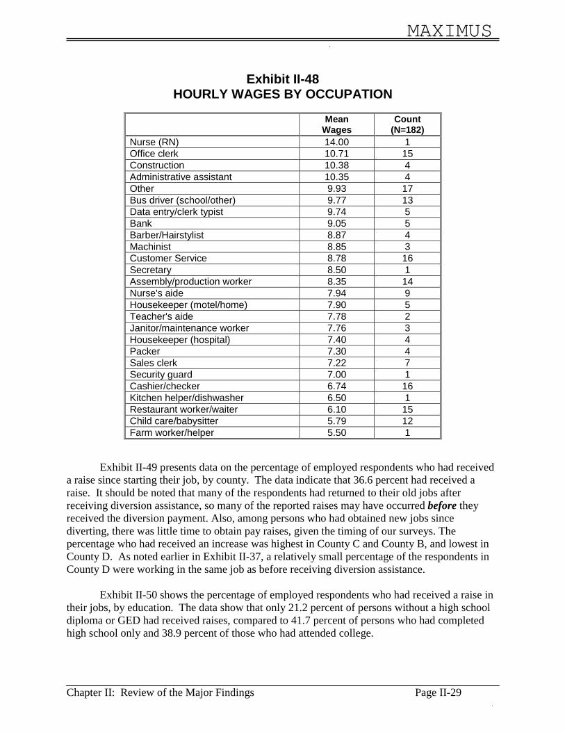
Exhibit II-48 shows monthly earnings by occupation. The data indicate that the highestpaying occupations were nurse, office clerk, construction, administrative assistant, bus driver,data entry, and bank worker, each of which averaged more than $9 per hour. The lowest payingoccupations were farmworker, child care/baby sitter, restaurant worker, and cashier/checker,each of which averaged less than $7 per hour. Jobs in houeskeeping, packing, nurse’s aid, andmaintenance averaged between $7 and $8 per hour.

Exhibit II-47MONTHLY WAGES OF EMPLOYED PERSONS, BY AGE

Less than22


Total

Less than $500 - - - 5.3% 6.7% 6.7% 2.7%$501 to $1,000 35.3% 10.3% 22.7% 26.3% 10.0% 13.3% 19.1%$1,001 to $1,500 52.9% 66.7% 45.5% 31.6% 26.7% 46.7% 44.8%More than $1,500 11.8% 20.5% 31.8% 36.8% 50.0% 26.7% 31.1%Total 100.0% 100.0% 100.0% 100.0% 100.0% 100.0% 100.0%

(N = 17) (N = 39) (N = 44) (N = 38) (N = 30) (N = 15) (N = 183)

MAXIMUS


Exhibit II-48HOURLY WAGES BY OCCUPATION

MeanWages

Count(N=182)

Nurse (RN) 14.00 1Office clerk 10.71 15Construction 10.38 4Administrative assistant 10.35 4Other 9.93 17Bus driver (school/other) 9.77 13Data entry/clerk typist 9.74 5Bank 9.05 5Barber/Hairstylist 8.87 4Machinist 8.85 3Customer Service 8.78 16Secretary 8.50 1Assembly/production worker 8.35 14Nurse's aide 7.94 9Housekeeper (motel/home) 7.90 5Teacher's aide 7.78 2Janitor/maintenance worker 7.76 3Housekeeper (hospital) 7.40 4Packer 7.30 4Sales clerk 7.22 7Security guard 7.00 1Cashier/checker 6.74 16Kitchen helper/dishwasher 6.50 1Restaurant worker/waiter 6.10 15Child care/babysitter 5.79 12Farm worker/helper 5.50 1

Exhibit II-49 presents data on the percentage of employed respondents who had receiveda raise since starting their job, by county. The data indicate that 36.6 percent had received araise. It should be noted that many of the respondents had returned to their old jobs afterreceiving diversion assistance, so many of the reported raises may have occurred before theyreceived the diversion payment. Also, among persons who had obtained new jobs sincediverting, there was little time to obtain pay raises, given the timing of our surveys. Thepercentage who had received an increase was highest in County C and County B, and lowest inCounty D. As noted earlier in Exhibit II-37, a relatively small percentage of the respondents inCounty D were working in the same job as before receiving diversion assistance.

Exhibit II-50 shows the percentage of employed respondents who had received a raise intheir jobs, by education. The data show that only 21.2 percent of persons without a high schooldiploma or GED had received raises, compared to 41.7 percent of persons who had completedhigh school only and 38.9 percent of those who had attended college.

MAXIMUS


Exhibit II-49PERCENTAGE OF EMPLOYED PERSONS WHO HAD RECEIVED A

RAISE IN THEIR PRIMARY JOB

County A County B County C County D Other TotalReceived raise 41.7% 50.0% 60.0% 24.8% 45.5% 36.6%

Did not receiveraise

58.3% 50.0% 40.0% 75.2% 54.5% 63.4%

Total 100.0% 100.0% 100.0% 100.0% 100.0% 100.0%


RAISE IN THEIR PRIMARY JOB, BY EDUCATION



Attendedcollege

Total

Received raise 21.2% 41.7% 38.9% 36.6%Did not receive raise 78.8% 58.3% 61.1% 63.4%Total 100.0% 100.0% 100.0% 100.0%

(N=33) (N=60) (N=90) (N=183)

Exhibit II-51 presents data on the percentage of employed respondents who had receivedpay raises, by ethnicity. The data indicate that a slightly higher percentage of non-whites (38.4percent) had received raises than whites (31.1 percent). This finding may be related to the datapresented earlier in Exhibit II-38 showing that non-whites were more likely to have returned totheir prior job than whites. In addition, as noted previously in Exhibit II-24, non-whites weremuch more likely than whites to have been working during the six months before receivingdiversion assistance.

Exhibit II-52 shows the percentage of employed respondents who had received a raise, byage. The data show that the youngest and the oldest respondents were generally the least likelyto have received a raise.


RAISE IN THEIR PRIMARY JOB, BY ETHNICITY

MAXIMUS


White Non-White TotalReceived raise 31.1% 38.4% 36.6%

Did not receive raise 68.9% 61.6% 63.4%Total 100.0% 100.0% 100.0%

(N = 45) (N = 138) (N = 183)


RAISE IN THEIR PRIMARY JOB, BY AGE

Less than22


Total

Received raise 29.4% 38.5% 25.0% 50.0% 46.7% 20.0% 36.6%

Did not receiveraise

70.6% 61.5% 75.0% 50.0% 53.3% 80.0% 63.4%

Total 100.0% 100.0% 100.0% 100.0% 100.0% 100.0% 100.0%(N = 17) (N = 39) (N = 44) (N = 38) (N = 30) (N = 15) (N = 183)

Exhibit II-53 shows the percentage of employed respondents who believed that therewere opportunities to move up in their current job. The data show that 48.6 percent thought thatthere were advancement opportunities. The percentage was highest in County B, County D, andCounty C, and lowest in County A and the three “other” counties.

Exhibit II-54 presents data on the how satisfied the employed respondents were with theircurrent jobs. The data indicate that 79.3 percent were very satisfied or somewhat satisfied. Thispercentage was lowest in County B (70.6 percent) and highest in the three “other” counties.

Exhibit II-53PERCENTAGE OF EMPLOYED PERSONS BELIEVING THAT THEREWERE ADVANCEMENT OPPORTUNITIES IN THEIR PRIMARY JOB

County A County B County C County D Other TotalAdvancementOpportunities

33.3% 58.8% 48.0% 50.5% 18.2% 48.6%

No Opportunities 66.7% 41.2% 52.0% 49.5% 81.8% 51.4%Total 100.0% 100.0% 100.0% 100.0% 100.0% 100.0%

MAXIMUS


Exhibit II-54DEGREE OF SATISFACTION WITH PRIMARY JOB

County A County B County C County D Other TotalVery satisfied 25.0% 32.4% 40.0% 35.6% 72.7% 37.2%Somewhat satisfied 66.7% 38.2% 40.0% 42.6% 27.3% 42.1%Neutral/no opinion 14.7% 16.0% 7.9% - 9.3%Somewhat dissatisfied 8.3% 14.7% 4.0% 4.0% - 6.0%Very dissatisfied - - - 9.9% - 5.5%Total 100.0% 100.0% 100.0% 100.0% 100.0% 100.0%

Exhibit II-55 shows the percentage of employed respondents who thought that theywould likely stay in their current jobs. Overall, almost half (48.2 percent) thought that theywould very likely stay in their current jobs and another 25.1 percent thought they would probablystay. The percentage who thought that they would very likely or probably stay in their jobs washighest in County C (84.0 percent) and the three “other” counties (81.8 percent).

For persons who indicated that they might not stay or probably would not stay in theircurrent jobs (n = 20), Exhibit II-56 shows the reasons why they might not stay. The mostcommon reason was low pay.

Exhibit II-55LIKELIHOOD OF STAYING IN PRIMARY JOB

County A County B County C County D Other TotalVery likely will stay 33.3% 38.2% 52.0% 52.5% 54.5% 48.6%Probably will stay 33.3% 32.4% 32.0% 19.8% 27.3% 25.1%Not sure 33.3% 14.7% 4.0% 15.8% 18.2% 15.3%Might not stay - 8.8% 12.0% 2.0% - 4.4%Very likely will not stay - 5.9% - 9.9% - 6.6%Total 100.0% 100.0% 100.0% 100.0% 100.0% 100.0%

Exhibit II-56MAIN REASON MAY NOT STAY IN PRIMARY JOB

Count(N=20)

Percentage

Low pay 8 40.0%No health insurance 1 5.0%No opportunity to advance/earn more money 3 15.0%Work hours not convenient 1 5.0%Might be laid off 1 5.0%

MAXIMUS


Does not like the job 2 10.0%Wants to own business 1 5.0%Wants to work in field of study 2 10.0%Other 1 5.0%

Exhibit II-57 presents data on the percentage of employed respondents who were workingfor an employer with a health care plan. The data show that 77.2 percent were working for anemployer with a health plan. However, the percentage was very low in County A (45.5 percent)compared to the other counties.

For respondents who were working for an employer with a health plan, Exhibit II-58shows the percentage of persons who were participating in the plan. The data show that only43.2 percent were participating. This percentage was highest in County C and County D andlowest in County B and the three “other” counties combined.

Combining the data from the two exhibits, we find that only one third (33.3 percent) ofemployed respondents were receiving health coverage through their employer (43.2 percent ofthe 77.2 percent who were working for an employer with a health plan). The percentage was41.7 percent in County C, 36.0 percent in County D, 29.4 percent in County B, and 18.2 percentin County A and the three “other” counties combined.

Exhibit II-57PERCENTAGE OF PERSONS WORKING FOR AN EMPLOYER WITH

HEALTH COVERAGE


Has Health Plan 45.5% 82.4% 79.2% 79.0% 72.7% 77.2%

Does not haveHealth Plan

54.5% 17.6% 20.8% 21.0% 27.3% 22.8%

Total 100.0% 100.0% 100.0% 100.0% 100.0% 100.0%

Exhibit II-58PERCENTAGE OF PERSONS PARTICIPATING IN THEIR

EMPLOYER'S COVERAGE


Participating 40.0% 35.7% 52.6% 45.6% 25.0% 43.2%Not Participating 60.0% 64.3% 47.4% 54.4% 75.0% 56.8%

MAXIMUS


Total 100.0% 100.0% 100.0% 100.0% 100.0% 100.0%

For respondents who reported that they were not participating in their employer’s healthplan (n = 79), Exhibit II-59 shows the reasons given for not participating. About 47 percent saidthat they had not worked for the employer long enough to qualify for health benefits. Almost 28percent indicated that the costs of the premiums were too high. About 37 percent indicated thatthey were still on Medicaid. The relatively short time frame between the diversion event and thefollow-up survey must be taken into account when considering the low percentage of employedrespondents who were covered by an employer health plan.

Exhibit II-59REASONS FOR NOT PARTICIPATING IN EMPLOYER'S HEALTH PLAN

Count(N=79)

Percentage

I haven't worked there longenough

37 46.8%

I'm a part-time employee 4 5.1%I'm a temporary employee 2 2.5%The cost is too high 22 27.8%I'm still on Medicaid 29 36.7%Don't know 2 2.5%Other 3 3.8%

DISCSSION OF THE FINDINGS

The surveys show relatively encouraging results in terms of the large percentage ofemployed respondents who were working 30 hours or more per week and who had earnings of$1,000 per month or more. The data also show relatively high rates of job satisfaction amongemployed respondents. On the other hand, about 22 percent of the sample were making less than$1,000 per month and 21 percent did not have a very high level of job satisfaction. About one-half did not see any opportunities for advancement in their current positions but about threequarters thought they would probably stay in their jobs.

The data showing that only about one third of all employed respondents wereparticipating in an employer health insurance plan also raises some concerns, although thispercentage may increase over time as more respondents begin to qualify for benefits at their jobs.The fact that about 39 percent of the respondents usually work on weekends raises potential

MAXIMUS


issues about child care availability. The data on occupations confirm that wages varyconsiderably in terms of the type of occupations in which low-income persons may be placed orfind jobs.

G. RECEIPT OF SERVICES, PUBLIC ASSISTANCE, AND OTHER BENEFITS SINCEDIVERTING

Exhibit II-60 shows the percentage of respondents who indicated that they had receiveddifferent types of training or other services since they obtained diversion assistance. About 13.7percent had received job training or education and 9.5 percent had received job placementassistance. Very few respondents had received transportation assistance, vocationalrehabilitation, substance abuse treatment, domestic violence assistance, or mental healthcounseling.

For those who had received job training or education, Exhibit II-61 shows who providedthe training or education. As indicated, about 27 percent received the training from theiremployer and 54.5 percent received training or education at a local college. Exhibit II-62 showsthe types of education or training that were received. Most of the training involved occupationalskills training and college courses.

Exhibit II-60PERCENTAGE OF PERSONS RECEIVING DIFFERENT TYPES OF

ASSISTANCE SINCE DIVERTING


Job Training oreducation

10.5% 18.6% 17.1% 10.8% 21.4% 13.7%

Job placementassistance

5.3% 11.6% 8.6% 8.5% 21.4% 9.5%

Transportationassistance

5.3% 7.0% 8.6% 3.8% - 5.0%

VocationalRehabilitation

- 2.3% - - - .4%

Substance abusetreatment

- 4.7% - .8% - 1.2%

Domestic violenceassistance

- 2.3% - - - .4%

Mental healthcounseling

5.3% 7.0% 5.7% .8% - 2.9%

Exhibit II-61ENTITY PROVIDING THE JOB TRAINING OR EDUCATION

Count Percentage

MAXIMUS


(N=33)County agency 1 3.0%Employer 9 27.3%Community/technical college or university 18 54.5%Job training provider 2 6.1%Other 3 9.1%

Exhibit II-62TYPE OF JOB TRAINING OR EDUCATION RECEIVED

Count(N=33)

Percentage

GED instruction or high schooldiploma

2 6.1%

English-as-a-Second Language(ESL)

1 3.0%

Occupational skills training 18 54.5%

Course(s) at a community/technical college or university

10 30.3%

Other 5 15.2%

Exhibit II-63 presents data on the receipt of various types of public assistance byrespondents at the time of the surveys. The data show that 55.8 percent of the respondents werereceiving Food Stamps at follow-up. The percentage was higher than average in County A (68.4percent) and lowest in the three “other” counties combined (35.7 percent). As indicatedpreviously in Exhibit II-26, County A had the lowest percentage of respondents who wereemployed at follow-up.

Exhibit II-63 also indicates that 80.6 percent of the respondents were receiving Medicaidfor themselves or their children at the time of the surveys. The percentage was very high in all ofthe counties except for County B, where only 59.1 percent were receiving Medicaid. We do nothave a clear explanation of why the rate of Medicaid participation in County B was so muchlower than in the other counties. As noted previously in Exhibit II-44, monthly wages amongemployed respondents in County B were higher than in the other counties, but this factor doesnot seem sufficient to explain the very low rate of Medicaid participation.

MAXIMUS


Exhibit II-63 also indicates that 8.3 percent of respondents were receiving assistanceunder the Section 8 housing program and 7.4 percent were in public housing. In County A, thepercentage of respondents who were receiving assistance with housing was much higher than inthe other counties (47.4 percent).

About 36.8 percent of respondents were participating in the WIC program. Thepercentage was very high in County B (56.8 percent) and relatively low in County D (30.0percent) and the three “other” counties combined (21.4 percent). The low rate of WICparticipation in the three “other” counties may be due to the fact that, as noted previously inExhibit II-18, none of the respondents in these counties was on maternity leave and very fewwere seeking assistance because of a new baby. In contrast, 40.9 percent of the respondents inCounty B were on maternity leave when they sought assistance.

Exhibit II-63PERCENTAGE OF RESPONDENTS RECEIVING DIFFERENT TYPES OF

BENEFITS AT FOLLOW-UP

County A CountyB

County C County D Other Total

Food Stamps 68.4% 50.0% 57.1% 57.7% 35.7% 55.8%

Medicaid (self orchild)

89.5% 59.1% 85.7% 84.6% 85.7% 80.6%

Section 8Certificate

21.1% 6.8% 8.6% 6.9% 7.1% 8.3%

Public housing 26.3% 11.4% 2.9% 4.6% 7.1% 7.4%

WIC Program 42.1% 56.8% 40.0% 30.0% 21.4% 36.8%

Transportation 5.3% 2.3% 2.9% 3.1% - 2.9%

SSI/SSDI (self orchildren)

5.3% 4.5% - 3.8% - 3.3%

Fuel/utilityAssistance

26.3% 4.5% - - - 2.9%

As noted in Exhibit II-63, very few of the respondents had received help withtransportation or fuel and utility assistance. Only 3.3 percent were receiving SSI/SSDI forthemselves or their children. This low rate of participation in the SSI and SSDI programsreflects that fact that diversion assistance is targeted primarily at persons without major barriersto employment.

Exhibit II-64 shows the percentage of respondents who were receiving different types ofbenefits at follow-up, by education. The data indicate that persons without a high schooldiploma were more likely to be receiving Food Stamps than other respondents. Persons who had

MAXIMUS


attended college were less likely to be receiving Medicaid or Section 8 assistance than otherrespondents. Persons without a high school diploma were less likely to be participating in WICthan more educated respondents, but were somewhat more likely to be receiving assistance withtransportation and fuel/utility assistance, and to be on SSI/SSDI.


BENEFITS AT FOLLOW-UP, BY EDUCATION

Did notcompleteHS/GED(N=47)


(N=78)

Attendedcollege(N=115)

Total(N=240)

Food Stamps 74.5% 52.6% 51.3% 56.3%Medicaid (self or child) 87.2% 87.2% 74.8% 81.3%Section 8 Certificate 10.6% 11.5% 5.2% 8.3%Public housing 6.4% 11.5% 5.2% 7.5%WIC Program 27.7% 44.9% 35.7% 37.1%Transportation 6.4% 3.8% .9% 2.9%SSI/SSDI (self or children) 6.4% 2.6% 2.6% 3.3%Fuel/utility Assistance 4.3% 2.6% 2.6% 2.9%

Exhibit II-65 shows the percentage of respondents receiving different types of assistance,by ethnicity. As indicated, there were no major differences between whites and non-whites inthe receipt of Food Stamps or Section 8 housing assistance. Whites were slightly more likely tobe receiving Medicaid than non-whites. In turn, non-whites were somewhat more likely to be inpublic housing and receiving WIC benefits.


BENEFITS AT FOLLOW-UP, BY ETHNICITY

White(N=70)

Non-white(N=172)

Total(N=242)

Food Stamps 58.6% 54.7% 55.8%

Medicaid (self or child) 85.7% 78.5% 80.6%Section 8 Certificate 7.1% 8.7% 8.3%Public housing 4.3% 8.7% 7.4%WIC Program 27.1% 40.7% 36.8%Transportation 1.4% 3.5% 2.9%SSI/SSDI (self or children) - 4.7% 3.3%

MAXIMUS


Fuel/utility Assistance 4.3% 2.3% 2.9%

Exhibit II-66 presents data on the receipt of public assistance, by age of the respondents.The data indicate that Medicaid participation was highest among persons under age 22. Thepercentage of respondents living in public housing was higher among the younger age groupsthan among older respondents. As expected, participation in WIC was much higher amongrespondents aged under 26 than among older respondents. Receipt of SSI/SSDI was muchhigher among the oldest age groups than among younger respondents.


BENEFITS AT FOLLOW-UP, BY AGE

Less than22

(N=20)

22 to 25(N=40)

26 to 30(N=49)

31 to 35(N=57)

36 to 40(N=56)

41 andover

(N=35)

Total(N=242)

Food Stamps 55.0% 71.4% 49.1% 57.1% 48.6% 48.0% 55.8%

Medicaid (self orchild)

95.0% 77.6% 80.7% 78.6% 82.9% 76.0% 80.6%

Section 8Certificate

5.0% 10.2% 7.0% 10.7% 5.7% 8.0% 8.3%

Public housing 25.0% 8.2% 10.5% 1.8% 2.9% 4.0% 7.4%

WIC Program 60.0% 69.4% 36.8% 30.4% 11.4% 4.0% 36.8%

Transportation - 2.0% 7.0% 1.8% - 4.0% 2.9%

SSI/SSDI (self orchildren)

- 2.0% 5.3% 1.8% - 12.0% 3.3%

Fuel/utilityAssistance

5.0% 4.1% 1.8% 1.8% 2.9% 4.0% 2.9%


The data show relatively low rates of participation in services such as job placement andtransportation assistance, but this might be expected in view of the fact that most of therespondents had recent work histories and had already returned to work. Although Food Stampsare part of the package of services designed to help recipients of Diversion Assistance, 44percent of the overall sample were not receiving Food Stamps at the time of the survey.However, this may reflect the fact that three-quarters of all respondents were employed atfollow-up and does not necessarily provide evidence of under-utilization of Food Stamps.Variations among counties in the rate of WIC participation may be related to differences in the

MAXIMUS


targeting of the Diversion Assistance program, but may also reflect differences in WIC outreachefforts.

H. USE OF CHILD CARE

Exhibit II-67 presents data on the use of child care (paid or unpaid) by respondents to thesurvey. The data show that 61 percent of the respondents were using child care. The percentagewas higher in County C (74.3 percent) and County B (65.1 percent) than in the other counties.

Exhibit II-67PERCENTAGE OF RESPONDENTS USING

PAID OR UNPAID CHILD CARE


Use Child Care 52.6% 65.1% 74.3% 58.5% 50.0% 61.0%

Do not use ChildCare

47.4% 34.9% 25.7% 41.5% 50.0% 39.0%

Total 100.0% 100.0% 100.0% 100.0% 100.0% 100.0%

For respondents who were not using child care, Exhibit II-68 shows the reasons given fornot using child care. Overall, 35.1 percent indicated that they were not working or in school andso did not need child care. About two-thirds of the respondents in County A cited this as areason for not using child care. Another 34 percent of all respondents indicated that they did notneed child care because their children were old enough to look after themselves. Another 18percent indicated that their spouse looked after their children. Only 5.3 percent cited problemswith being able to afford child care as the reason for not using child care. Only 3.2 percentmentioned problems finding a child care provider that met their needs.

Exhibit II-69 presents data on the types of child care used by respondents. Overall, about47 percent of persons who were using child care were using a child care center. The percentageusing a child care center was relatively high in County B, County D, and the three “other”counties combined, and relatively low in County A and County C. The next most common typeof provider was “paid relative or friend – not living in the home,” accounting for about one-fifthof all providers. Another 10.2 percent were using a relative or friend who was not living in thehome and who was not being paid. About 7.5 percent were using a day care home and 6.1percent were using a school-based program.

MAXIMUS


Exhibit II-68REASONS FOR NOT USING CHILD CARE


I'm not working orattending school

66.7% 40.0% 44.4% 31.5% - 35.1%

My children are old enoughto look after themselves

22.2% 26.7% - 38.9% 71.4% 34.0%

I can't afford to pay forchild care

11.1% 6.7% 11.1% 3.7% - 5.3%

I can't find a child careprovider that meets myneeds

11.1% - 11.1% 1.9% - 3.2%

Spouse cares for children - 13.3% 33.3% 20.4% 14.3% 18.1%Other - 20.0% 11.1% 7.4% 14.3% 9.6%

Exhibit II-69TYPE OF CHILD CARE PROVIDER FOR PERSONS USING CHILD

CARE


Relative living inhome – paid

- 7.1% - 1.3% - 2.0%

Relative living inhome – unpaid

20.0% 3.6% - 2.6% - 3.4%

Relative or friend notliving in home – paid

20.0% 25.0% 15.4% 19.7% 14.3% 19.7%

Relative or friend notliving in home –unpaid

20.0% - 19.2% 10.5% - 10.2%

Day careCenter

30.0% 50.0% 30.8% 52.6% 57.1% 46.9%

School program(before/after schoolcare)

10.0% - 15.4% 3.9% 14.3% 6.1%

Family child carehome

- 14.3% 7.7% 6.6% - 7.5%

Other - - 11.5% 2.6% 14.3% 4.1%

Total 100.0% 100.0% 100.0% 100.0% 100.0% 100.0%

MAXIMUS


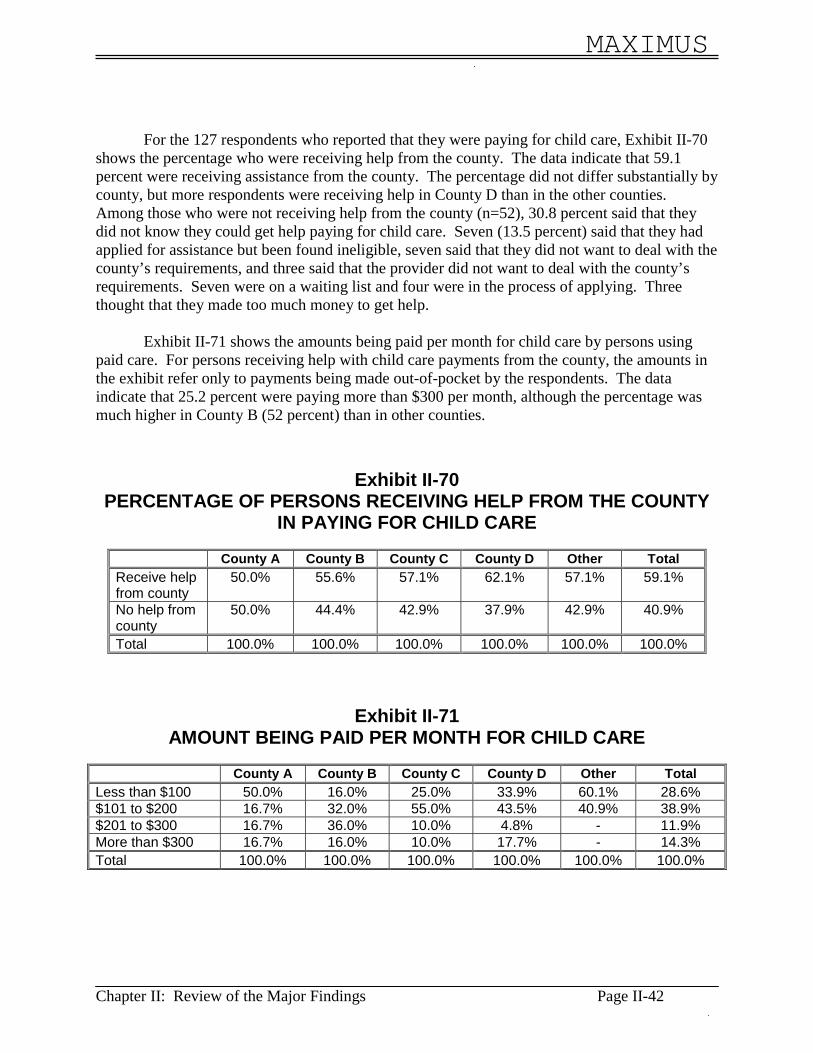
For the 127 respondents who reported that they were paying for child care, Exhibit II-70shows the percentage who were receiving help from the county. The data indicate that 59.1percent were receiving assistance from the county. The percentage did not differ substantially bycounty, but more respondents were receiving help in County D than in the other counties.Among those who were not receiving help from the county (n=52), 30.8 percent said that theydid not know they could get help paying for child care. Seven (13.5 percent) said that they hadapplied for assistance but been found ineligible, seven said that they did not want to deal with thecounty’s requirements, and three said that the provider did not want to deal with the county’srequirements. Seven were on a waiting list and four were in the process of applying. Threethought that they made too much money to get help.

Exhibit II-71 shows the amounts being paid per month for child care by persons usingpaid care. For persons receiving help with child care payments from the county, the amounts inthe exhibit refer only to payments being made out-of-pocket by the respondents. The dataindicate that 25.2 percent were paying more than $300 per month, although the percentage wasmuch higher in County B (52 percent) than in other counties.

Exhibit II-70PERCENTAGE OF PERSONS RECEIVING HELP FROM THE COUNTY

IN PAYING FOR CHILD CARE


Receive helpfrom county

50.0% 55.6% 57.1% 62.1% 57.1% 59.1%

No help fromcounty

50.0% 44.4% 42.9% 37.9% 42.9% 40.9%

Total 100.0% 100.0% 100.0% 100.0% 100.0% 100.0%

Exhibit II-71AMOUNT BEING PAID PER MONTH FOR CHILD CARE


Less than $100 50.0% 16.0% 25.0% 33.9% 60.1% 28.6%$101 to $200 16.7% 32.0% 55.0% 43.5% 40.9% 38.9%$201 to $300 16.7% 36.0% 10.0% 4.8% - 11.9%More than $300 16.7% 16.0% 10.0% 17.7% - 14.3%Total 100.0% 100.0% 100.0% 100.0% 100.0% 100.0%

MAXIMUS



Access to subsidized child care is potentially an important component of diversionprograms. “Diversionary” child care can help prevent persons from leaving jobs or turning downjobs because of lack of access to affordable or convenient child care. Child care subsidies canalso be important for job retention after a diversion client finds a job. The surveys showed that,although 39 percent of the overall sample were not using child care, most of these respondentsdid not feel that they needed child care, either because they were not working or because of theages of their children. Relatively few of the respondents indicated that they were not using childcare because of problems with affordability or access. In addition, of those who were using childcare, only about 35 percent were relying on “informal” child care arrangements through familymembers or friends.

The fact that about 41 percent of the families who were using paid child care were notreceiving help from the county is a potential concern, especially since about 31 percent of thesedid not know that they could get help. Another 13.5 percent were on waiting lists.

I. RECEIPT OF CHILD SUPPORT

Exhibit II-72 presents data on the percentage of respondents who were receiving childsupport at the time of the surveys. As indicated, 17.9 percent were receiving child support and82.1 percent were not. The percentage who were receiving child support did not varysubstantially among the counties, except that a much higher percentage of respondents in thethree “other” counties combined were receiving support. When interpreting the data, it must bekept in mind that 19.4 percent of the respondents were living with their spouses (see Exhibit II-7). Adjusting for this, about 22.3 percent of respondents who were not living with their spouseswere receiving child support.

Exhibit II-72PERCENTAGE OF RESPONDENTS RECEIVING CHILD SUPPORT


Receive childsupport

15.8% 18.6% 17.1% 17.1% 28.6% 17.9%

Do not receivechild support

84.2% 81.4% 82.9% 82.9% 71.4% 82.1%

Total 100.0% 100.0% 100.0% 100.0% 100.0% 100.0%

Exhibit II-73 shows the percentage of respondents who were receiving child support, byethnicity. The data show that there was not a major difference between whites and non-whites inthe percentage of respondents who were receiving child support. Exhibit II-74 shows the

MAXIMUS


percentage who were receiving child support, by education. The data indicate that persons whohad completed high school or attended college were more than twice as likely to be receivingchild support as persons who had not completed high school.

Exhibit II-73PERCENTAGE OF RESPONDENTS RECEIVING CHILD SUPPORT,

BY ETHNICITY

White Non-White TotalReceive childsupport

17.4% 18.1% 17.9%

Do not receive childcupport

82.6% 81.9% 82.1%

Total 100.0% 100.0% 100.0%(N = 69) (N = 171) (N = 240)

Exhibit II-74PERCENTAGE OF RESPONDENTS RECEIVING CHILD SUPPORT,

BY EDUCATION



Attendedcollege

Total

Receive childSupport

8.5% 21.8% 19.1% 17.9%


91.5% 78.2% 80.9% 82.1%

Total 100.0% 100.0% 100.0% 100.0%(N = 47) (N = 78) (N = 115) (N = 240)

Exhibit II-75 presents data on the percentage of respondents who were receiving childsupport, by age. The data indicate that persons aged 41 and over were less likely to be receivingchild support than younger respondents. Persons aged under 22 were also somewhat less likelyto be receiving child support than the average respondent.

Among persons who were receiving child support (n = 43), 25.6 percent said they werereceiving $100 per month or less. Another 25.6 percent were receiving $101 to $200; 18.6percent were receiving $201 to $300; 20.9 percent were receiving $301 to $500; and 9.3 percentwere receiving more than $500 per month.

Exhibit II-75

MAXIMUS


PERCENTAGE OF RESPONDENTS RECEIVING CHILD SUPPORT,BY AGE

Less than22


Total

Receive childsupport

15.0% 22.4% 14.3% 21.4% 20.0% 8.3% 17.9%


85.0% 77.6% 85.7% 78.6% 80.0% 91.7% 82.1%

Total 100.0% 100.0% 100.0% 100.0% 100.0% 100.0% 100.0%(N = 20) (N = 49) (N = 56) (N = 56) (N = 35) (N = 24) (N = 240)


Effective child support enforcement is a potentially important component of efforts todivert welfare applicants from cash assistance. Child support, if paid consistently, can helpreduce the family’s reliance on welfare. Under welfare reform, efforts by states to divertapplicants from welfare have usually been accompanied by greater emphasis on expediting andstrengthening child support enforcement activities. The fact that only 22 percent of respondentswho were not living with their spouses were receiving any child support suggests thatenforcement may need to be strengthened to make diversion efforts more feasible for a greaterpercentage of welfare applicants.

J. HEALTH CARE AND HEALTH INSURANCE

Exhibit II-76 presents data on the percentage of respondents who reported that they had aregular place where they took their child(ren) for medical care and check-ups. As indicated,about 90.8 percent of the respondents reported that they did have a regular place to take theirchildren. The percentage was somewhat lower in County D (85.3 percent) than in the othercounties. This may have reflected the refugee population in the County D sample.

For those respondents who had a regular place to take their children, Exhibit II-77 showsthe place where respondents usually took their children for medical care. Slightly more than halftook their children to a clinic, but the percentage was lower in County A and higher in County D.About 35.8 percent took their children to a private physician, but the percentage was muchhigher in County A, County C, and the three “other” counties, and lower in County B andCounty D.

Exhibit II-76PERCENTAGE OF RESPONDENTS REPORTING THAT THEY HAD A

REGULAR PLACE TO TAKE CHILDREN FOR MEDICAL CARE


Have a regular place 94.7% 100.0% 94.3% 85.3% 100.0% 90.8%Do not have a 5.3% - 5.7% 14.7% - 9.2%

MAXIMUS


regular placeTotal 100.0% 100.0% 100.0% 100.0% 100.0% 100.0%

Exhibit II-77PLACE WHERE RESPONDENTS USUALLY TOOK CHILDREN FOR

MEDICAL CARE


Private physician 61.1% 30.2% 48.5% 27.3% 57.1% 35.8%HMO - 11.6% 6.1% 13.6% - 10.1%Clinic 33.3% 51.2% 45.5% 57.3% 42.9% 51.4%Emergency room 5.6% - - .9% - .9%Other - 7.0% - .9% - 1.8%Total 100.0% 100.0% 100.0% 100.0% 100.0% 100.0%

Exhibit II-78 shows the percentage of respondents who reported that their children werecovered by a medical plan. About 91.6 percent of all respondents reported that their childrenwere covered by a medical plan. However, only 79.1 percent of respondents in County Breported that their children were covered.

For respondents whose children were covered by a medical plan, Exhibit II-79 shows thetype of health plan involved. Respondents could indicate more than one option. About 91.8percent of the children were covered by Medicaid or Health Choices. Combining this numberwith the 91.6 percent of respondents whose children were covered by a health plan, we find thatchildren were covered by Medicaid or Health Choices in about 84.1 percent of all cases. InCounty B, only 65.2 percent of children were covered by Medicaid or Health Choices. However,children in County B were somewhat more likely to be covered by the parent’s employer healthinsurance than in the other counties.

Exhibit II-78PERCENTAGE OF RESPONDENTS WHOSE CHILDREN ARE

COVERED UNDER A MEDICAL PLAN


Covered underMedical Plan

100.0% 79.1% 94.3% 93.0% 100.0% 91.6%

Not Covered underMedical Plan

- 20.9% 5.7% 7.0% - 8.4%

MAXIMUS


Total 100.0% 100.0% 100.0% 100.0% 100.0% 100.0%

Exhibit II-79TYPE OF HEALTH INSURANCE PLAN FOR COVERED CHILDREN


Medicaid or HealthChoices

89.5% 85.3% 93.9% 93.3% 92.9% 91.8%

Health insurancethrough employer

5.3% 11.8% 6.1% 9.2% 7.1% 8.7%

Health insurancefrom the children'sother parent

5.3% 5.9% 6.1% .8% - 2.7%


The data do not show any major issues with health care access or coverage for the largemajority of children in the different counties. However, the data for County B suggest that moreof the respondents in the sample may encounter health coverage problems over time as theyobtain jobs and potentially lose their coverage for their children under Medicaid or HealthChoices. Many of these persons may not be able to find jobs that have employer health plans ormay not be eligible immediately to participate in these plans.

K. DEPRIVATION, OVERALL FINANCIAL SITUATION, AND FUTURE NEEDS

Respondents were asked a series of questions designed to assess their material andfinancial well-being in the context of their decision to accept diversion assistance. The keyfindings are presented below.

Deprivation and Food Security

Respondents were asked whether they had experienced various types of deprivation(including problems buying food) either before or after they had received diversion assistance.Exhibit II-80 presents data on reported deprivation, by county. It should be noted that the timeperiod before receiving diversion assistance is open-ended, while the time period since receivingdiversion assistance is constrained by the timing of the surveys.

The data show that 34.7 percent reported getting behind in paying their rent or mortgagesince diverting, and that 37.9 percent had experienced this problem before diverting. About 17.5percent reported that, since diverting, they had on occasion needed medical care for a family

MAXIMUS


member but could not afford it. This was an increase from 12.5 percent in the period beforediverting. About 14.6 percent reported that, since diverting, they had on occasion needed childcare but could not pay for it. Relatively small percentages reported other types of deprivation,such as having to move in with a relative, take in a boarder, stay in a homeless shelter, or gowithout utilities.

About 21.7 percent reported that, since diverting, there were times when they had no wayto buy food. About 26.3 percent reported that there were times before they diverted when theyhad no way to but food.

Exhibit II-80RESPONDENTS REPORTING DIFFERENT EVENTS

BEFORE OR AFTER DIVERTING

BeforeDiverting

SinceDiverting

Got behind in paying for rent or mortgage 37.9% 34.2%Moved because could not pay for housing 10.0% 4.6%Moved in with a friend or relative 17.5% 5.0%Took in a boarder or relative 0.8% 3.3%Went without heat, electricity, or water in home 5.4% 6.3%Stayed in a homeless shelter 3.3% 0.4%Placed children with someone else 4.2% 1.3%Placed children in foster care 0.4% -Needed routine child care but could not pay for it 16.3% 14.6%Needed medical care for a family member but couldnot pay

12.5% 17.5%

Had times when had no way to buy food 26.3% 21.7%

Exhibit II-81 presents data on the percentage of respondents who reported various typesof deprivation since diverting from welfare, by county. The data show that no major differencesexisted among the counties for many of the deprivation indicators. However, persons in CountyA were more likely to report problems paying for child care than persons in other counties. Nomajor differences existed among the counties in the percentage who reported being unable to payfor medical care at some time. Respondents in County B and County D were much more likelyto report problems paying for food than persons in other counties.

Exhibit II-81RESPONDENTS REPORTING DIFFERENT EVENTS SINCE DIVERTING

MAXIMUS



Got behind in payingfor rent or mortgage

36.8% 41.9% 20.0% 34.9% 35.7% 34.2%

Moved because couldnot pay for housing

- 4.7% 2.9% 6.2% - 4.6%

Moved in with a friendor relative

5.3% 4.7% 7.0% - 5.0%

Took in a boarder orrelative

5.3% 7.0% 5.7% 1.6% - 3.3%

Went without heat,electricity, or water inhome

5.3% 4.7% 8.6% 7.0% - 6.3%

Stayed in a homelessshelter

- 0.8% - 0.4%

Placed children withsomeone else

- 4.7% 2.9% - 1.3%

Placed children infoster care

- 0.8% - 0.4%

Needed routine childcare but could not payfor it

26.3% 14.0% 11.4% 15.5% - 14.6%

Needed medical carefor a family member butcould not pay

15.8% 18.6% 17.1% 17.8% 14.3% 17.5%

Had times when had noway to buy food

10.5% 30.2% 11.4% 24.0% 14.3% 21.7%

Exhibit II-82 presents data on reported deprivation since diverting, by ethnicity. The datashow that non-whites were about twice as likely as whites to report having needed medical carefor a family member but not having been able to pay. As noted previously in Exhibit II-65, non-whites were slightly less likely to be covered by Medicaid (78.5 percent) than whites (85.7percent). However, as noted in Exhibit II-27, non-whites were also more likely to be employedat follow-up than whites. It is possible that a number of non-whites may have lost Medicaidcoverage for themselves due to employment, but may not have been covered by an employerhealth plan.

The exhibit also shows that non-whites were much more likely than whites to reporthaving had times when the had no way to buy food. Almost one-quarter of non-whites reportedfood insecurity, compared to 14.5 percent of whites. On most of the other deprivation measures,non-whites were slightly more likely than whites to report deprivation.

MAXIMUS


Exhibit II-82RESPONDENTS REPORTING DIFFERENT EVENTS

SINCE DIVERTING, BY ETHNICITY

White Non-White TotalGot behind in paying for rent ormortgage

31.9% 35.1% 34.2%

Moved because could not pay forhousing

2.9% 5.3% 4.6%

Moved in with a friend or relative 4.3% 5.3% 5.0%Took in a boarder or relative 2.9% 3.5% 3.3%Went without heat, electricity, orwater in home

2.9% 7.6% 6.3%

Stayed in a homeless shelter - 0.6% 0.4%Placed children with someone else - 1.8% 1.3%Placed children in foster care - 0.6% 0.4%Needed routine child care but couldnot pay for it

15.9% 14.0% 14.6%

Needed medical care for a familymember but could not pay

10.0% 20.5% 17.5%

Had times when had no way to buyfood

14.5% 24.6% 21.7%

For those respondents who reported that there had been times when they had no way tobuy food, Exhibit II-83 shows the actions taken to address the situation. The data show that themost common action taken both before and after diversion was to ask friends or relatives forfood or money. This action was taken by about 69 percent of respondents who had problemsbuying food. Since diverting, only one of the respondents said that they went hungry. About 9.6percent (n = 5) had obtained food from a shelter or food pantry.

Exhibit II-83ACTIONS TAKEN BY RESPONDENTS WHEN THEY DID NOT HAVE

MONEY FOR FOOD, BEFORE AND AFTER DIVERTING

Actions Taken

BeforeDiverting

(N=63)

SinceDiverting

(N=52)Went hungry 6.3% 1.9%

Got meals or food at shelter/foodkitchen/food pantry

15.9% 9.6%

Got meals/food/money for food from church 28.6% 17.3%Were given food or money for food byfriends/relatives

69.8% 69.2%

Other 6.3% 7.7%

MAXIMUS


Housing Adequacy

Exhibit II-84 presents data relevant to possible housing overcrowding among therespondents. The exhibit shows the number of rooms in the respondent’s home, excludingbathrooms. Only 6.3 percent indicated that they had three rooms or less. The data, therefore, donot provide any significant evidence of housing overcrowding among the sample.

Exhibit II-85 presents data on problems reported by respondents with housing conditions.Overall, 13.6 percent reported problems with water leakage, with the percentage being highestamong County C respondents. About 14.9 percent reported problems with open cracks or holesin the walls or ceilings, including more than one-third of persons in the three “other” countiescombined. Residents in the “other” counties were also more likely to report broken or missingwindows. Relatively few respondents reported security problems with their homes.

Exhibit II-84NUMBER OF ROOMS IN RESPONDENT'S HOUSE


1 - 3 rooms 5.3% 4.7% 2.9% 8.5% - 6.3%4 rooms 47.4% 44.2% 51.4% 41.1% 35.7% 43.3%5 rooms 31.6% 34.9% 31.4% 32.6% 42.9% 33.3%6 or more 15.8% 16.3% 14.3% 17.8% 21.4% 17.1%Total 100.0% 100.0% 100.0% 100.0% 100.0% 100.0%

Exhibit II-85PERCENTAGE OF RESPONDENTS REPORTING

HOUSING DEFECTS


Portable roomheater

5.3% 6.8% 8.6% 7.7% 7.1% 7.4%

Water leakage - 13.6% 20.0% 13.8% 14.3% 13.6%

Open cracks orholes

- 15.9% 14.3% 14.6% 35.7% 14.9%

Broken plaster 5.3% 2.3% 8.6% 13.1% - 9.1%

Broken/ missingwindows

5.3% 6.8% 5.7% 7.7% 14.3% 7.4%

Heating or ACproblems

15.8% 6.8% 5.7% 12.3% 7.1% 10.3%

Electrical problems 5.3% 4.5% - 10.8% - 7.0%Security problemsfor self/family

- 4.5% - 8.5% 7.1% 5.8%

MAXIMUS


Overall Financial Situation

Respondents were asked how well their family’s current income and benefits met theirfamily’s needs. Exhibit II-86 presents the findings by county. As indicated, 19.2 percent feltthat their income and benefits met their family’s needs with some left over, and another 34.2percent felt that their needs were being met with nothing left over. About 27.1 percent believedthat their income and benefits nearly met their needs, and 19.6 percent felt that their needs weredefinitely not being met.

The percentage who felt that their needs were being met, with or without some left over,was about the same in County B, C, and D (50-52 percent), but higher in County A (57.9percent) and the three “other” counties (71.4 percent). The percentage who felt that their needswere clearly not being met was much higher in County C (37.1 percent) than in the othercounties. Overall, the percentage who believed that their needs were not being met (last twocategories combined) was about the same in County B, C, and D (48-49 percent) and lower inthe other counties.

Exhibit II-86HOW WELL FAMILY'S INCOME AND BENEFITS

MEET THE FAMILY'S NEEDS


Meet Needs withSome Left Over

26.3% 20.9% 17.1% 17.8% 21.4% 19.2%

Meet Needs withNothing Left Over

31.6% 30.2% 34.3% 34.1% 50.0% 34.2%

Nearly Meet Needs 21.1% 30.2% 11.4% 31.0% 28.6% 27.1%

Does Not MeetNeeds

21.1% 18.6% 37.1% 17.1% - 19.6%

Total 100.0% 100.0% 100.0% 100.0% 100.0% 100.0%

Other Household Income

Respondents were asked about other family income besides their own earnings andbenefits. Only five percent of the respondents reported that they personally had income besidestheir earnings and the public assistance benefits described earlier in Exhibit II-63. Thisadditional income included gifts of money from family and friends, as well as more formal typesof income.

MAXIMUS


However, many of the respondents reported that there were other adults in thehousehold who had income. Exhibit II-87 shows that slightly more than one third of thehouseholds included another adult who was working for pay. In total, 111 respondents reportedthat they had other adults living with them (first two rows in the exhibit). In these 111 familiescombined, there were 145 other adults besides the respondent. Of these 145 other adults, 93were reported to be working for pay.

Exhibit II-87PERCENTAGE OF HOUSEHOLDS IN WHICH THERE WAS

ANOTHER ADULT WORKING FOR PAY

Count(N=240)

Percentage

Other adult in home, andworking

77 32.1%

Other adult in home, notworking

34 14.2%

No other adult in home 129 53.8%

Future Needs

Respondents were asked to identify anticipated needs for specific services in the nearfuture. Exhibit II-88 shows that about 40 percent of the respondents were anticipating a need foremergency food or clothing, including 53.5 percent of respondents in County B but relativelyfew in County A and the smaller counties. About 36.7 percent anticipated a need for housingassistance, including almost 42 percent in County D and about 35 percent in County B. Slightlymore than one quarter felt that they would need job counseling or job search assistance, with thehighest percentages being in County C and County A. (As noted previously in Exhibit II-26,County A had the lowest percentage of respondents who were employed at the time of thesurvey).

Exactly 50 percent thought they would need help with child care, including 60.5 percentin County B and 57.9 percent in County A. About 27.5 percent anticipated a need fortransportation assistance, including one third of all County D respondents. Relatively fewrespondents anticipated a need for substance abuse treatment, domestic violence counseling, ormental health counseling.

Almost 30 percent of the respondents thought that they would need help with householdbudgeting, including 36.4 percent of persons in County D. Slightly more than 40 percent feltthat they would have a need for job training or education, including relatively high percentagesin County A, County C, and County D. Finally, 50 percent of all respondents said that theywould need help with child support enforcement. The percentage was fairly standard across thecounties.

MAXIMUS



Overall, the findings indicate that there is some evidence of deprivation and lack of foodsecurity among the respondents, but there is no evidence of major problems in such areas asfamilies going hungry, becoming homeless, living in substandard or overcrowded housing, orhaving to place children elsewhere. Persons who reported problems obtaining enough food toeat were generally able to find food from family members, friends, or food pantries. However,the fact that a significant percentage of persons reported problems buying food (30 percent inCounty B and 24 percent in County D) may be cause for concern, especially since diverters aresupposed to be persons who need minimal income support or other services. The data also raisesome concerns about medical coverage for certain segments of the population.

Part of the reason why there is little evidence of deprivation is that most respondentswere employed and about 39 percent had other adults in the household who were working. Interms of future needs, the data confirm that many respondents see a need for improved childsupport enforcement.

Exhibit II-88ANTICIPATED NEEDS OF RESPONDENTS IN THE FUTURE


Emergency foodor clothing

26.3% 53.5% 37.1% 40.3% 21.4% 40.0%

Housingassistance

31.6% 34.9% 31.4% 41.9% 14.3% 36.7%

Job counselingor job searchassistance

31.6% 25.6% 34.3% 26.4% 7.1% 26.7%

Child careassistance

57.9% 60.5% 51.4% 48.1% 21.4% 50.0%

Transportationassistance

26.3% 25.6% 17.1% 33.3% 7.1% 27.5%

Substanceabuse treatment

- 2.3% - - - .4%

Domesticviolenceassistance

- - - .8% - .4%

Mental healthcounseling

5.3% 2.3% 5.7% 8.5% - 6.3%

Householdbudgetingassistance

15.8% 25.6% 22.9% 36.4% 7.1% 29.2%

Job training oreducation

42.1% 32.6% 42.9% 43.4% 35.7% 40.8%

Child support 47.4% 55.8% 51.4% 47.3% 57.1% 50.0%

MAXIMUS


assistance

L. LIKELIHOOD OF REAPPLYING FOR WELFARE

Exhibit II-89 presents data on what respondents thought about their likelihood ofreapplying for welfare in the next six months. About 40.8 percent thought it very unlikely thatthey would reapply. This percentage did not vary much by county. Another 12.9 percentthought it somewhat unlikely that they would reapply. A total of 17.1 percent said that it wasvery likely or somewhat likely that they would reapply for welfare. The percentage who thoughtit “very likely” that they would reapply was highest in County C, County B and County D.

Exhibit II-89LIKELIHOOD OF REAPPLYING FOR WELFARE


Very likely 5.3% 14.0% 17.1% 11.6% - 11.7%Somewhat likely 10.5% 7.0% 4.7% 14.3% 5.4%Not sure 21.1% 30.2% 25.7% 27.9% 35.7% 27.9%Somewhat unlikely 15.8% 9.3% 11.4% 14.0% 14.3% 12.9%Very unlikely 42.1% 39.5% 45.7% 40.3% 35.7% 40.8%Already applied 5.3% - - 1.6% - 1.3%Total 100.0% 100.0% 100.0% 100.0% 100.0% 100.0%

Exhibit II-90 presents data on the likelihood of reapplying for welfare, by education. Thedata indicate that 19.1 percent of persons who had not completed high school and 21.7 percent ofthose who had only completed high school thought it very likely or somewhat likely that theywould reapply for welfare in the future. This compares to only 13.0 percent of persons who hadattended college.

Exhibit II-90LIKELIHOOD OF REAPPLYING FOR WELFARE, BY EDUCATION



Attendedcollege

Total

Very likely 8.5% 17.9% 8.7% 11.7%Somewhat likely 10.6% 3.8% 4.3% 5.4%

MAXIMUS


Not sure 38.3% 21.8% 27.8% 27.9%Somewhat unlikely 2.1% 16.7% 14.8% 12.9%Very unlikely 38.3% 38.5% 43.5% 40.8%Already applied 2.1% 1.3% .9% 1.3%Total 100.0% 100.0% 100.0% 100.0%

(N = 47) (N = 78) (N = 115) (N = 240)

Exhibit II-91 shows the likelihood of reapplying for welfare, by ethnicity. About 14percent of non-whites thought that they were very likely to reapply, compared to only 5.8 percentof whites. However, the percentage who were not likely to reapply or who were not sure was notvery different between the two groups.

Exhibit II-92 shows the likelihood of reapplying for welfare, by age. The data do notshow any clear pattern of age differences, except that persons in the 36 to 40 age group were lesslikely to reapply than the other age groups.

Exhibit II-91LIKELIHOOD OF REAPPLYING FOR WELFARE, BY ETHNICITY

White Non-White TotalVery likely 5.8% 14.0% 11.7%

Somewhat likely 8.7% 4.1% 5.4%Not sure 27.5% 28.1% 27.9%Somewhat unlikely 14.5% 12.3% 12.9%Very unlikely 42.0% 40.4% 40.8%Already applied 1.4% 1.2% 1.3%Total 100.0% 100.0% 100.0%

(N = 69) (N = 171) (N = 240)

Exhibit II-92LIKELIHOOD OF REAPPLYING FOR WELFARE, BY AGE

Less than22


Total

Very likely 10.0% 12.2% 12.5% 14.3% 5.7% 12.5% 11.7%Somewhat likely 10.0% 8.2% 3.6% 8.6% 8.3% 5.4%Not sure 40.0% 32.7% 21.4% 25.0% 22.9% 37.5% 27.9%Somewhat unlikely 10.2% 17.9% 19.6% 5.7% 12.5% 12.9%Very unlikely 40.0% 34.7% 44.6% 37.5% 57.1% 29.2% 40.8%Already applied - 2.0% - 3.6% - - 1.3%Total 100.0% 100.0% 100.0% 100.0% 100.0% 100.0% 100.0%

(N = 20) (N = 49) (N = 56) (N = 56) (N = 35) (N = 24) (N = 240)

MAXIMUS


Exhibit II-93 presents data on the likelihood of reapplying for welfare, by the age of theyoungest child. Welfare researchers have often found that persons with young children are morelikely to go back on welfare than other former recipients. The data in the exhibit do not showany clear relationship between age of the youngest child and the perceived likelihood ofreapplying for welfare. Persons whose youngest child was 3 to 5 were the least likely to thinkthat they would reapply.

Finally, Exhibit II-94 presents data on the likelihood of reapplying for welfare, bywhether the respondent had been on welfare before. As indicated, 14.0 percent of persons whohad been on welfare before thought it very likely that they would be reapplying, compared toonly 9.8 percent of persons who had not been on welfare before. Of those who had been onwelfare, 48.6 percent thought that it was somewhat unlikely or very unlikely that they wouldreapply, compared to 57.9 percent of persons who had not been on welfare.

Exhibit II-93LIKELIHOOD OF REAPPLYING FOR WELFARE,

BY AGE OF THE YOUNGEST CHILD

Less thanone year

1 to 2years

3 to 5years

6 to 8years

Over 9years

Total

Very likely 10.4% 13.5% 6.5% 18.9% 11.9% 11.7%Somewhat likely 6.5% 2.7% 4.3% 5.4% 7.1% 5.4%Not sure 31.2% 27.0% 19.6% 32.4% 28.6% 28.0%Somewhat unlikely 14.3% 16.2% 17.4% 5.4% 9.5% 13.0%Very unlikely 36.4% 40.5% 50.0% 35.1% 42.9% 40.6%Already applied 1.3% - 2.2% 2.7% - 1.3%Total 100.0% 100.0% 100.0% 100.0% 100.0% 100.0%

(N = 77) (N = 37) (N = 46) (N = 37) (N = 42) (N = 239)

Exhibit II-94LIKELIHOOD OF REAPPLYING FOR WELFARE,

BY WHETHER ON WELFARE BEFORE

On WelfareBefore


Total

Very likely 14.0% 9.8% 11.7%

Somewhat likely 4.7% 6.0% 5.4%Not sure 30.8% 25.6% 27.9%Somewhat unlikely 9.3% 15.8% 12.9%Very unlikely 39.3% 42.1% 40.8%Already applied 1.9% .8% 1.3%Total 100.0% 100.0% 100.0%

MAXIMUS


(N = 107) (N = 133) (N = 240)

Reasons for Reapplying

Among respondents who thought that they were very likely or somewhat likely to reapplyfor welfare, 43.9 percent cited “loss of job or lack of a job” as the most probable reason.Another 7.3 percent mentioned a decrease in work hours or wages. About 14.6 percent citedhousing problems. Only 7.3 percent mentioned child support problems and only 4.9 percentcited transportation problems.


Overall, the data are relatively encouraging in terms of the low percentage of respondentswho feel that they are unlikely to reapply for welfare. However, in County B, County C, andCounty D, between 11 percent and 17 percent of respondents thought it very likely that theywould reapply. The data suggest that there may be a segment of the diverter population thatneeds to be screened more effectively before being referred to the Diversion Assistance program.This population may include persons who have been on welfare before for extensive periods oftime, especially if they do not have high school diplomas.

M. SATISFACTION WITH THE DIVERSION DECISION

Respondents were asked how satisfied they were with the decision to accept diversionassistance, including the amount of the diversion payment. Exhibit II-95 shows that two-thirdsof all respondents were “very satisfied” with the diversion decision and that another 20 percentwere somewhat satisfied. Only 6.3 percent were either dissatisfied or very dissatisfied. Thepercentage who were dissatisfied was highest in County A and County B. However, County Aalso had the highest percentage of respondents who were very satisfied with the decision.

Exhibit II-96 presents data on the level of satisfaction with the amount of the diversionpayment. Overall, 51.7 percent were very satisfied and 37.1 percent were somewhat satisfied.No major differences existed among the counties, except that County B respondents weresomewhat less satisfied than respondents in other counties.

Exhibit II-97 presents data on levels of satisfaction with the amount of the diversionpayment, by ethnicity. The data indicate that whites were slightly more likely than non-whites tobe very satisfied with the amount of the diversion payment, but there was not a major differencebetween the two groups.

MAXIMUS


Exhibit II-95SATISFACTION WITH THE DIVERSION DECISION


Very satisfied 84.2% 53.5% 74.3% 67.4% 57.1% 66.7%Somewhat satisfied 5.3% 30.2% 11.4% 20.2% 28.6% 20.0%Neutral/no opinion 7.0% 11.4% 6.2% 14.3% 7.1%Somewhat dissatisfied 10.5% 7.0% - 3.1% - 3.8%Very dissatisfied 2.3% 2.9% 3.1% - 2.5%Total 100.0% 100.0% 100.0% 100.0% 100.0% 100.0%

Exhibit II-96SATISFACTION WITH THE AMOUNT OF THE DIVERSION PAYMENT


Very satisfied 57.9% 41.9% 54.3% 53.5% 50.0% 51.7%Somewhat satisfied 36.8% 44.2% 45.7% 32.6% 35.7% 37.1%Neutral/no opinion - 7.0% - 4.7% 14.3% 4.6%Somewhat dissatisfied 5.3% 4.7% - 6.2% - 4.6%Very dissatisfied - 2.3% - 3.1% - 2.1%Total 100.0% 100.0% 100.0% 100.0% 100.0% 100.0%

Exhibit II-97SATISFACTION WITH THE AMOUNT OF THE DIVERSION PAYMENT,

BY ETHNICITY

White Non-white TotalVery satisfied 56.5% 49.7% 51.7%

Somewhat satisfied 36.2% 37.4% 37.1%Neutral/no opinion 4.3% 4.7% 4.6%Somewhat dissatisfied 2.9% 5.3% 4.6%Very dissatisfied - 2.9% 2.1%Total 100.0% 100.0% 100.0%

(N = 69) (N = 171) (N = 240)

Exhibit II-98 shows the percentage of respondents who believed that they were better offat the time of the survey than before they received diversion assistance. The data show thatabout one quarter considered themselves much better off than before and another 37.1 percentthought they were a little better off. Only 6.2 percent thought that they were worse off, including10.1 percent of persons in County D. The percentage who thought that they were much better

MAXIMUS


off or a little better off did not vary by county except that the percentages were higher in thethree “other” counties combined.

Exhibit II-99 presents data on whether respondents thought that they were better off, byethnicity. The data show that non-whites were less likely than whites to think that they weremuch better off. However, not much difference exists between the two groups in the percentagewho thought that they were either much better off or a little better off (68.1 percent for whitesand 60.2 percent for non-whites). There was not a major difference between the two groups inthe percentage of persons who thought that they were worse off.

Exhibit II-98RESPONDENTS’ VIEWS OF THEIR OVERALL SITUATION

SINCE DIVERTING


Much better off 26.3% 23.3% 28.6% 23.3% 42.9% 25.4%A little better off 31.6% 34.9% 31.4% 39.5% 42.9% 37.1%About the same 36.8% 39.5% 40.0% 27.1% 14.3% 31.3%A little worse off 5.3% 2.3% - 8.5% - 5.4%Much worse off - - - 1.6% - .8%Total 100.0% 100.0% 100.0% 100.0% 100.0% 100.0%

Exhibit II-99RESPONDENTS’ VIEWS OF THEIR OVERALL SITUATION

SINCE DIVERTING, BY ETHNICITY

White Non-White TotalMuch better off 33.3% 22.2% 25.4%

A little better off 34.8% 38.0% 37.1%About the same 24.6% 33.9% 31.3%A little worse off 7.2% 4.7% 5.4%Much worse off - 1.2% .8%Total 100.0% 100.0% 100.0%

(N = 69) (N = 171) (N = 240)


The data show that, despite evidence of deprivation among some segments of thepopulation, the large majority of participants were satisfied with their decision to divert from

MAXIMUS


welfare. The majority were also satisfied with the amount of the diversion payment. The factthat 13 percent were not satisfied with the diversion decision may indicate a need for morecareful screening by counties in referring certain applicants to the program.

Documents

CHAPTER II: REVIEW OF THE MAJOR FINDINGS · MAXIMUS Chapter II: Review of the Major Findings Page II-2 Exhibit II-1 GENDER OF THE RESPONDENT