Chapter 9 Hypothesis Testing II - King's Facultydkerr.kingsfaculty.ca/dkerr/assets/File/StatsL92205.pdf · 2019. 3. 12. · 3/12/2019 10 9-19 The obtained test statistic (Z = 20)

3/12/2019

1

9-1

This week:

Hypothesis Testing II:

Chapter 8: The Two-Sample Case

Chapter 10: Hypothesis testing: Chi square

REVIEWS THIS WEDNESDAY & FRIDAY DURING NORMAL

TUTORIAL TIMES!

CHANGE IN SCHEDULE:

Problem solving Assignment # 4 due 11:30 a.m.

sharp – 6%

Change from March 19th to March 26th (DUE)

9-2

Chapter 7: Last week

Hypothesis Testing:

The One-Sample Case Compare a sample statistic

with a population parameter

We take a sample of Brock students; calculate a statistic

(mean GPS),

& then ask: do they differ significantly from

all students in Ontario (the population parameter)?

3/12/2019

2

9-3

Chapter 7: before text

Hypothesis Testing:

The One-Sample Case

TODAY: Chapter 8:

Hypothesis Testing II:

The Two-Sample Case

Compare a sample statistic

with a population parameter

Compare a sample statistic

with another sample statistic

We take a sample of Brock students; calculate a statistic

(mean GPS),

& then ask: do they differ significantly from

all students in Ontario (the population parameter)?

• The basic logic of the two sample case.

• Hypothesis Testing with

Sample Means (Large Samples),

Sample Means (Small Samples)

Sample Proportions (Large Samples)

• The difference between “statistical significance” and “importance”

• A few more words on setting “alpha”

• Bivariate tables and Chi square (Chapter 10) 9-4

In this presentation

you will learn about:

3/12/2019

3

9-5

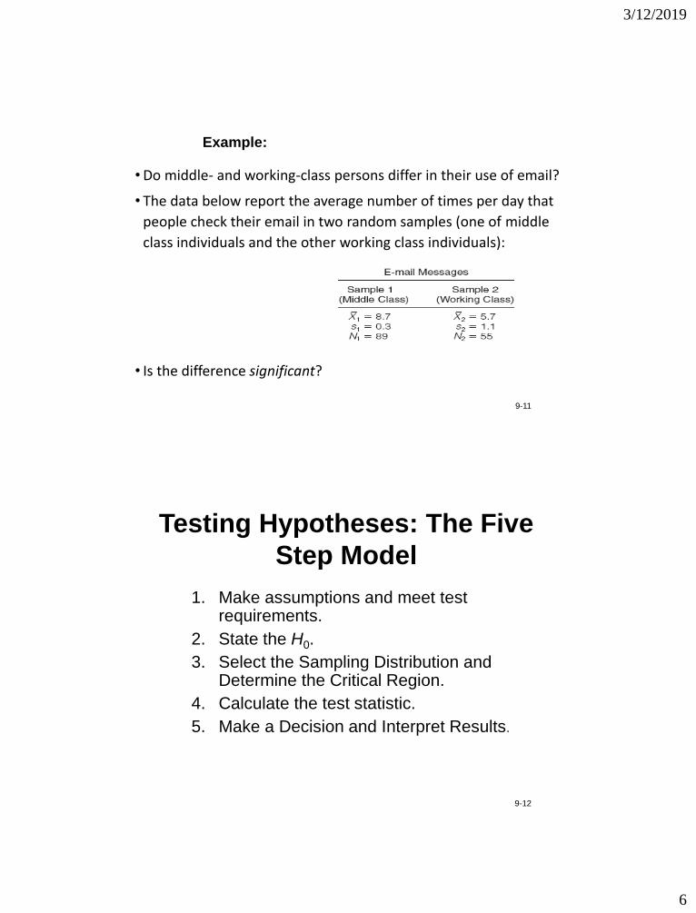
• Do middle- and working-class persons differ in their use of email?

• The data below report the average number of times per day that

people check their email in two random samples (one of middle

class individuals and the other working class individuals):

• The middle class seem to check their email more than the

working class, but is the difference significant?

Example:

We begin with a difference between sample statistics (means).

The question we test: “Is the difference between the samples large enough to allow us to

conclude (with a known probability of error) that the populations represented by the samples are different?”

Hypothesis Test for Two Samples: Basic Logic

The null hypothesis, H0, is that the samples represent

populations that are the same:

There is no difference between the parameters of the two

populations. H0: μ1 = μ2

If the difference between the sample statistics is large enough,

or, if a difference of this size is unlikely assuming H0 is true, we reject the H0

Conclude that there is a significant difference between the populations.

H1: μ1 μ2 or or

H1: μ1 > μ2 H1: μ1 < μ2

3/12/2019

4

9-7

• Step 1: in addition to samples selected according to EPSEM principles, samples must be selected independently: Independent random sampling.

• Step 2: null hypothesis statement will say the two populations are not different.

• Step 3: sampling distribution refers to difference between the sample

statistics.

• Step 4: In computing the test statistic, we use Z(obtained) or t(obtained) with slightly revised formula, depending on the size of our sample (forthcoming)

• Step 5: same as before: If the test statistic, Z(obtained) or t(obtained), falls into the critical region, as marked by Z(critical) or t(critical), reject the H0.

Changes from One- to Two-Sample Case

9-8

• Step 4: In computing the test statistic, we use Z(obtained) or

t(obtained) with slightly revised formula, depending on the size

of our sample (forthcoming)

We will work with 3 options & 3 sets of formulae

1. If comparing sample means (2 large samples)

1a. With population standard deviations

1b. With only sample standard deviations

2. If comparing sample means (small samples: n1 and n2 < 100)

3. If comparing sample proportions (large samples)

NOTE: STEP 4 USES DIFFERENT FORMULA!!!

3/12/2019

5

9-9

1a. If comparing sample means (2 large samples) with σ

2. If sample means (small samples)

3. If sample proportions (large samples)

21

2211

nn

PnPnP ss

u

21

21)1(nn

nnuupp

1b. If comparing sample means (2 large samples) with s

with

with

with

9-10

3/12/2019

6

9-11

• Do middle- and working-class persons differ in their use of email?

• The data below report the average number of times per day that

people check their email in two random samples (one of middle

class individuals and the other working class individuals):

• Is the difference significant?

Example:

9-12

1. Make assumptions and meet test requirements.

2. State the H0.

3. Select the Sampling Distribution and Determine the Critical Region.

4. Calculate the test statistic.

5. Make a Decision and Interpret Results.

Testing Hypotheses: The Five

Step Model

3/12/2019

7

9-13

Return to our example:

9-14

• Model:

• Independent Random Samples • The samples must be independent of each other (i.e. the selection of cases in the

first sample has no bearing on the selection of cases in the second)

• Level of Measurement is Interval-Ratio • Number of email messages -> can work with our means

• Sampling Distribution’s shape • N = (85+55 =144) cases which is > 100 so we can assume a normal shape.

Step 1: Make Assumptions and

Meet Test Requirements

3/12/2019

8

9-15

• No direction for the difference has been predicted, so a two-tailed test is called for, as reflected in the research hypothesis:

• H0: μ1 = μ2 • The Null asserts there is no significant difference between the populations (the

two populations represented by our samples are equally likely to be using email)

• H1: μ1 μ2 • The research hypothesis contradicts the H0 and asserts there is a significant

difference between the populations.

Step 2: State the Null Hypothesis

• Sampling Distribution = Z distribution

• Alpha (α) = 0.05

• note: unless otherwise stated, use 0.05 in all significance tests (i.e. the default in most tests)

• With two tailed test: Z (critical) = ± 1.96

Step 3: Select Sampling Distribution and Establish the

Critical Region

Step 4: Compute the Test Statistic

With two sample tests, use the appropriate formula (below) to

compute the obtained Z score:

The denominator in this formula is the standard deviation

of the sampling distribution (i.e. the standard error)

3/12/2019

9

9-17

NOTE: How do we calculate this standard error that enters into the denominator of Z(obtained)?

When the population standard deviations are known, we use the following formula:

but when we only have the sample standard deviations, we use the following:

i.e. we substitute s as an estimator of σ, suitably corrected for the bias (n is replaced by n-1 to correct for the fact that s is a biased estimator of σ).

Again, the above formula only apply if the combined size of the two samples is at least N> 100

Step 4 (continued)

9-18

So: calculate standard error (population standard deviations unknown):

On this basis, you can calculate Z (obtained) with the standard error in

the denominator

In this example: compute the Test Statistic

15.022.001.155

1.1

189

3.

11

222

2

2

1

21

n

s

n

s

20

15.

7.57.821

Z

We have the “sample standard

deviations”,..

3/12/2019

10

9-19

The obtained test statistic (Z = 20) falls in the Critical Region so reject the null hypothesis.

• The difference between the sample means is so large that we can conclude, at α = 0.05, that a difference exists between the populations represented by the samples.

• The difference between email usage of middle- and working-class individuals is significant.

Step 5: Make Decision and Interpret Results

20

9-20

Hypothesis Test for Two-Sample

Means: Student’s t distribution (Small Samples)

3/12/2019

11

9-21

• For small samples (combined N’s<100), s is too unreliable an estimator of σ so do not use standard normal distribution. Instead we use Student’s t distribution.

• The formula for computing the test statistic, t(obtained), is:

where is defined as:


Means: Student’s t distribution (Small Samples)

9-22

• The logic of the five-step model for hypothesis testing is followed, using the t table, Appendix B, where the degrees of freedom (df) = N1 + N2 – 2.


Means: Student’s t distribution (continued)

3/12/2019

12

9-23

Example: Research on Obesity,.. How to deal with the problem?

9-24

•

Example: Studying “weight loss” strategies:

1st sample – combined cardio (30 minutes a day & weight

training 30 minutes a day)

Mean weight loss: 20 pounds

s =5

Sample size (n1 = 29)

2nd sample – Solely cardio (45 minutes a day)

Mean weight loss: 18 pounds

s = 4

Sample size (n2 = 33)

Is there a significant difference between the two??

3/12/2019

13

9-25

• Model:

• Independent Random Samples

• Level of Measurement is Interval-Ratio • Weight loss-> can work with our means

• Sampling Distribution’s shape • N = (29+33=62) cases which is less than 100 so we must work with t distribution

Step 1: Make Assumptions and

Meet Test Requirements

9-26

• No direction for the difference has been predicted, so a two-tailed test is called for, as reflected in the research hypothesis:

• H0: μ1 = μ2 • The Null asserts there is no significant difference in the weight loss for the two

populations

• H1: μ1 μ2 • The research hypothesis contradicts the H0 and asserts there is a significant

difference in weight loss


3/12/2019

14

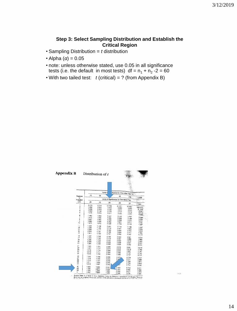
• Sampling Distribution = t distribution

• Alpha (α) = 0.05

• note: unless otherwise stated, use 0.05 in all significance tests (i.e. the default in most tests) df = n1 + n2 -2 = 60

• With two tailed test: t (critical) = ? (from Appendix B)


Critical Region

9-28

3/12/2019

15

• Sampling Distribution = t distribution

• Alpha (α) = 0.05

• note: unless otherwise stated, use 0.05 in all significance tests (i.e. the default in most tests) df = N1 + N2 -2 = 60

• With two tailed test: t (critical) = ± 2.00 (from Appendix B)


Critical Region

Step 4: Compute the Test Statistic

With two sample tests, use the appropriate formula (below) to

compute the obtained t score:

BUT: must first calculate the denominator (SE)

NOTE: How do we calculate this standard error ?

When the population standard deviations are unknown, we use Formula 8.5 to calculate :

Again, the above formula only apply if the combined size of the two samples is less than 100

Step 4 (continued)

21

21

21

21

2

2

2

2

1

nn

nn

nn

snsn

)33)(29(

3329

23329

)4)(33()5)(29( 22

= 1.16

3/12/2019

16

9-31

On this basis, you can calculate t (obtained) with the standard error in

the denominator

In this example: compute the Test Statistic

72.1

16.1

1820)(

21

obtainedt

9-32

The obtained test statistic (t = 1.72) does not fall in the Critical Region so we can not reject the null hypothesis.

Recall: t(critical) +/- 2.0

• The difference between the sample means is not large enough that we can

• conclude, at α = 0.05, that a difference exists between the populations represented by the samples.

•

• The difference between the two populations using the different exercise regimes is NOT significant.


-2.0 2.0

1.72

3/12/2019

17

9-33

TWO sample test with Proportions (or percentages)….

We conduct research on educational outcomes

AFN’s National Chief, Perry Bellegarde has urged the Trudeau

Government to act on “education”!!

Example: Sample from Non-Aboriginal Population (N=60) Ps1 = .23 (23 % are university educated) Sample from Aboriginal Population (N=72) Ps2 = .10 (10% are university educated) Are Non-Aboriginal Canadians significantly more likely than Aboriginal Canadians to have a university degree? Problem here: can we infer from our samples, that are not that large?

3/12/2019

18

Formula for Hypothesis Testing with Sample Proportions (Large Samples)

• Formula for proportions:

Where Ps1 is the proportion associated with the first sample, and Ps2 is the proportion associated with the second.

• See next slide for how to calculate the denominator in this equation (standard error)* and the “pooled estimate of the population proportion”*….

• *Note that you need to calculate both these values in order to solve the denominator of the above equation!

pp

ssobtained

21)(

To obtain standard error, most first calculate something called: Pu (the Pooled Estimate of the Population Proportion)

• To calculate Pu (the pooled estimate, see p. 255):

• Which is then inserted into the following equation for the standard deviation of the sampling distribution (standard error):

21

21)1(nn

nnuupp

21

2211

nn

PnPnP ss

u

Which then enters into the aforementioned formula for

our test statistic Z(obtained)

3/12/2019

19

9-37

Again, use the basic 5 step model in testing for significance…

Step 1. Model has independent random samples, Level of measurement is “nominal” -> work with proportions Sampling distribution can be considered normal since N> 100 Step 2. State null hypothesis: direction? Yes, one tailed test H0: Pμ1 = Pμ2

The Null asserts there is no significant difference in the proportion with a university degree for the two populations H1: Pμ1 > Pμ2

The research hypothesis contradicts the H0 and asserts there is a significant difference: Non-Aboriginal people have a higher education.. Than Aboriginal Canadians..

3/12/2019

20

Step 3. Select the sampling distribution and establish critical region Sampling distribution is the Z distribution Alpha is .05 one tailed Appendix A table indicates Z(critical) = 1.65

Step 4. Calculate the test statistic Start with “pooled estimate on the proportion”

21

2211

nn

PnPnP ss

u

159.7260

)10)(.72()23)(.60(

uP

21

21)1(nn

nnuupp

Next: get our standard error

064.0)72)(60(

7260)159.1(159.

pp

3/12/2019

21

Step 4 (continued)

Then obtain your test statistic:

pp

ssobtained

21)(

031.2064.

10.23.)(

obtained

9-42

The obtained test statistic Z = 2.031) falls in the Critical Region so we can reject the null hypothesis.

Recall: Z(critical) +1.65

• The difference between the proportions is large enough to conclude, at α = 0.05, that Non-Aboriginal Canadians are significantly more likely to have a university education than “Aboriginal Canadians”

• The difference between the two populations is significant.


2.031

1.65

3/12/2019

22

8-43

• By assigning an alpha level, α, one defines an “unlikely” sample outcome.

• Alpha level is the probability that the decision to reject the null hypothesis, H0, is incorrect.

• If we set our Alpha at .05, and we end up rejecting our

null hypothesis,.. We are 95% certain that we are correct

If we set our Alpha at .10, and we end up rejecting our

null hypothesis, we are 90% certain that we are correct..

Etc…

Do note: that our sampling distribution tells us that sometimes we can be

wrong!!

Some comments on Alpha Levels

8-44

Alpha levels affect Critical Region in Step 3:

3/12/2019

23

9-45

• The probability of rejecting the null hypothesis in comparing statistics is a function of four independent factors:

1.The size of the difference (e.g., means of 8.7 and 5.7 for the example above).

2.The value of alpha (the higher the alpha, the more likely we are to reject the H0).

3.The use of one- vs. two-tailed tests (we are more likely to reject with a one-tailed test).

4.The size of the sample (N ) (the larger the sample the more likely we are to reject the H0).

Significance vs. Importance

9-46

• As long as we work with random samples, we must conduct a test of significance. However, significance is not the same thing as importance.

• Differences that are otherwise trivial or uninteresting may be significant, which is a major limitation of hypothesis testing. ◦ When working with large samples, even small differences may be significant.

◦ The value of the standard error is always an inverse function of N (i.e. the larger the N, the smaller the standard error)

◦ The larger the N, the greater the value of the test statistic (standard error is always in the denominator), the more likely it will fall in the Critical Region and be declared significant.

Significance vs. Importance (continued)

3/12/2019

24

9-47

• In conclusion, significance is a necessary but not sufficient condition for importance.

• A sample outcome could be:

• significant and important

• significant but unimportant (e.g. with a very large N)

• not significant but important (yikes: hazard of small N)

• not significant and unimportant

Significance vs. Importance (continued)

11-48

Next Chapter: Chapter 10

Hypothesis Testing IV:

Chi Square

3/12/2019

25

• Bivariate (Cross tabulation) Tables

• The basic logic of Chi Square

• If time:

• Perform the Chi Square test using the five-step model

11-49

In this presentation

you will learn about:

11-50

Why examine a “bivariate table”? Example: We are conducting research on smoking & education.. Small sample (N=600), is there a significant association??

3/12/2019

26

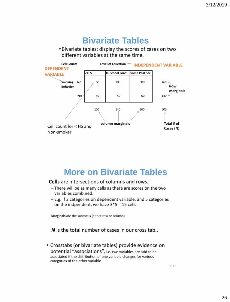
• Bivariate tables: display the scores of cases on two different variables at the same time.

column marginals

Bivariate Tables

Row marginals

Total # of Cases (N)

Cell Counts Level of Education

< H.S. H. School Grad Some Post Sec

Smoking No 60 100 300 460

Behavior

Yes 40 40 60 140

100 140 360 600

INDEPENDENT VARIABLE DEPENDENT VARIABLE

Cell count for < HS and Non-smoker

11-52

Cells are intersections of columns and rows. – There will be as many cells as there are scores on the two

variables combined. – E.g. If 3 categories on dependent variable, and 5 categories

on the indpendent, we have 3*5 = 15 cells Marginals are the subtotals (either row or column)

N is the total number of cases in our cross tab..

• Crosstabs (or bivariate tables) provide evidence on potential “associations”, i.e. two variables are said to be associated if the distribution of one variable changes for various categories of the other variable

More on Bivariate Tables

3/12/2019

27

11-53

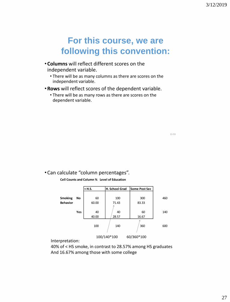
• Columns will reflect different scores on the independent variable.

• There will be as many columns as there are scores on the independent variable.

• Rows will reflect scores of the dependent variable. • There will be as many rows as there are scores on the

dependent variable.

For this course, we are

following this convention:

• Can calculate “column percentages”.

100/140*100 60/360*100 Interpretation: 40% of < HS smoke, in contrast to 28.57% among HS graduates And 16.67% among those with some college

Cell Counts and Column % Level of Education


Smoking No 60 100 300 460

Behavior 60.00 71.43 83.33

Yes 40 40 60 140

40.00 28.57 16.67

100 140 360 600

3/12/2019

28

If dependent variable is in your rows.. USE column % in interpretation.. The row %’s can potentially be very misleading..

If dependent variable happened to be in your columns, you would have to use the “row %” in interpretation!!

11-55

11-56

What if?

Sample of 690 clerical workers (1980)

Independent

Women Men total

Dependent

smokers 65 45 110

non-smokers 500 80 580

Total 565 125 690

Row % or Column %???

3/12/2019

29

11-57

What if?


Independent

Women Men total

Dependent

smokers 65 45 110


Total 565 125 690

Independent

Women Men total

Dependent

smokers 59.1% 40.9% 100.0%

non-smokers 86.2% 13.8% 100.0%

Total

Independent

Women Men total

Dependent

smokers 11.5% 36.0%

non-smokers 88.5% 64.0%

Total 100.0% 100.0%

OR?

Row %

Column %

11-58

What if?


Independent

Women Men total

Dependent

smokers 65 45 110


Total 565 125 690

Independent

Women Men total

Dependent

smokers 59.1% 40.9% 100.0%

non-smokers 86.2% 13.8% 100.0%

Total

Independent

Women Men total

Dependent

smokers 11.5% 36.0%

non-smokers 88.5% 64.0%

Total 100.0% 100.0%

OR?

Row %

Column %

X

3/12/2019

30

11-59

Cell Counts and Column % Level of Education


Smoking No 60 100 300 460

Behavior 60.00 71.43 83.33

Yes 40 40 60 140

40.00 28.57 16.67

100 140 360 600

Smoking

No Yes Total

<H.S 60 40 100

60.0 40.0

H. School Grad 100 40 140

71.4 28.6

Some Post Sec. 300 60 360

83.3 16.7

Total 460 140 600

OR (the exact same data) – both are okay, right?:

Column %

Row %

Level of education

11-60

• Interpret this table:

Interpretation Not obvious with counts.. Can calculate column percentages to aid in interpretation since dependent variable is in the rows Also: formal test of significance is possible… (chi square)

Dependent variable

Independent variable

Incidence and % of Obesity by Province, 2008

Nfld PEI NS NB Quebec

Obese 173,298 36,998 230,913 229,299 1,739,628

Not Obese 336,402 105,302 711,588 522,501 6,167,772

Total 509,700 142,300 942,500 751,800 7,907,400

3/12/2019

31

Interpretation?

An association “appears to exist” between province of residence and obesity; the distribution of obese and non-obese vary across provinces e.g. 34% of Nfld are obese, as apposed to only 22% of Quebec residents NOTE: VERY LARGE #s here: LIKELY REAL!!!



Obese 173,298 36,998 230,913 229,299 1,739,628

34.00% 26.00% 24.50% 30.50% 22.00%

Not Obese 336,402 105,302 711,588 522,501 6,167,772

66.00% 74.00% 75.50% 69.50% 78.00%

Total 509,700 142,300 942,500 751,800 7,907,400

100.00% 100.00% 100.00% 100.00% 100.00%

What if we are working with relatively small numbers?

• Can we be sure an association (relationship) really exists for the larger population even if the %’s differ ???

11-62

• Numbers here are quite small.. Might the variation merely

be the by-product of sampling error?

• There is a formal test to see whether the differences are

significant or not -> chi square test..



Obese 17 4 23 23 17

33.33% 26.67% 24.47% 30.67% 21.52%

Not Obese 34 11 71 52 62

66.67% 73.33% 75.53% 69.33% 78.48%

Total 51 15 94 75 79

3/12/2019

32

11-63

Our Chi Square test is also called, the Chi Square test of “Independence”…. What do we mean by “Independence” in this context? The opposite of having an “association between two variables”… i.e. an absence of any type of association or relationship

• With this table? Is there a relationship between the two variables??

Males are no more likely to

participate than Females NO RELATIONSHIP

“Independence”

o Two variables are independent if the classification of a case into a particular category of one variable has no effect on the probability that the case will fall into any particular category of the second variable.

100

50

150

66.7

33.3

100

3/12/2019

33

o Let us return to our example with education and smoking… Cell Counts and Column % Level of Education


Smoking No 60 100 300 460

Behavior 60.00 71.43 83.33

Yes 40 40 60 140

40.00 28.57 16.67

100 140 360 600

o Complete “Independence” would look like:

Some

< HS H.School Grad Post sec

Smoking behavior

No 77 107 276 460

77% 77% 77%

Yes 23 33 84 140

23% 23% 23%

100 140 360 600

23%

77% Expected frequencies, if we had independence..

77%

23%

100%

11-66

Again, a fundamental 5 step model!!! Question to answer: Does an “association” really exist? (given N) Or do we have “independence”?

Chi Square, χ2, is a test of significance based on bivariate, cross tabulation tables.

Chi Square is a test for independence.

Specifically, we are looking for significant differences between the observed cell frequencies in a table (fo) and those that would be expected by random chance or if cell frequencies were independent (fe):

Basic Logic of Chi Square TEST

3/12/2019

34

11-67

Formulas for Chi Square

.. Gives us our “expected frequencies” under assumption of “independence”

Formal test statistic Step 4!

• Is there a relationship between support for

privatization of healthcare and political ideology? Are

liberals significantly different from conservatives on

this variable? o The table below reports the relationship between these two variables

for a random sample of 78 adult Canadians.

Computation of Chi Square:

An Example

Political Ideology Support Conservative Liberal Total No 14 29 43 Yes 24 11 35 Total 38 40 78

3/12/2019

35

11-69

How do we calculate our “test statistic” in our chi squared test of independence?

Must first use:

And then calculate:

11-70

Use Formula 10.2 to find fe.

– To obtain fe multiply column and row

marginals for each cell and divide by N. • (38*43)/78 = 1634 /78 = 20.9 • (40*43)/78 = 1720 /78 = 22.1 • (38*35)/78 = 1330 /78 = 17.1 • (40*35)/78 = 1400 /78 = 17.9

Expected frequencies (fe)

Political Ideology

Support Conservative Liberal Total

No 20.9 22.1 43

Yes 17.1 17.9 35

Total 38 40 78

An Example (continued)

Observed Frequencies (fo) Conservative Liberal Total No 14 29 43 Yes 24 11 35 Total 38 40 78

3/12/2019

36

11-71

Political Ideology


No 20.9 22.1 43

Yes 17.1 17.9 35

Total 38 40 78

Example:


Observed: (f0)

Expected frequencies (fe) OUR test statistic tells us whether these are Significantly different!!

11-72

•A computational table helps organize the computations.

fo fe fo - fe (fo - fe)2 (fo - fe)

2 /fe

14 20.9

29 22.1

24 17.1

11 17.9

78 78

Example (continued)

TOTAL

3/12/2019

37

11-73

•Subtract each fe from each fo. The total of this column must be zero.


2 /fe

14 20.9 -6.9

29 22.1 6.9

24 17.1 6.9

11 17.9 -6.9

78 78 0 TOTAL

11-74

•Square each of these values


2 /fe

14 20.9 -6.9 47.61

29 22.1 6.9 47.61

24 17.1 6.9 47.61

11 17.9 -6.9 47.61

78 78 0 TOTAL

3/12/2019

38

11-75

• Divide each of the squared values by the fe for that cell. The sum of this column is chi square


2 /fe

14 20.9 -6.9 47.61 2.28

29 22.1 6.9 47.61 2.15

24 17.1 6.9 47.61 2.78

11 17.9 -6.9 47.61 2.66

78 78 0 χ2 = 9.87

Computation of Chi Square: An Example (continued)

TOTAL

What to do with this chi square? 9.87? The larger the chi square, the more likely the association is significant We need a formal test…

11-76

What about our “sampling distribution” and “critical score” in our Formal test? Here, we use a sampling distribution called the CHI square sampling distribution….

3/12/2019

39

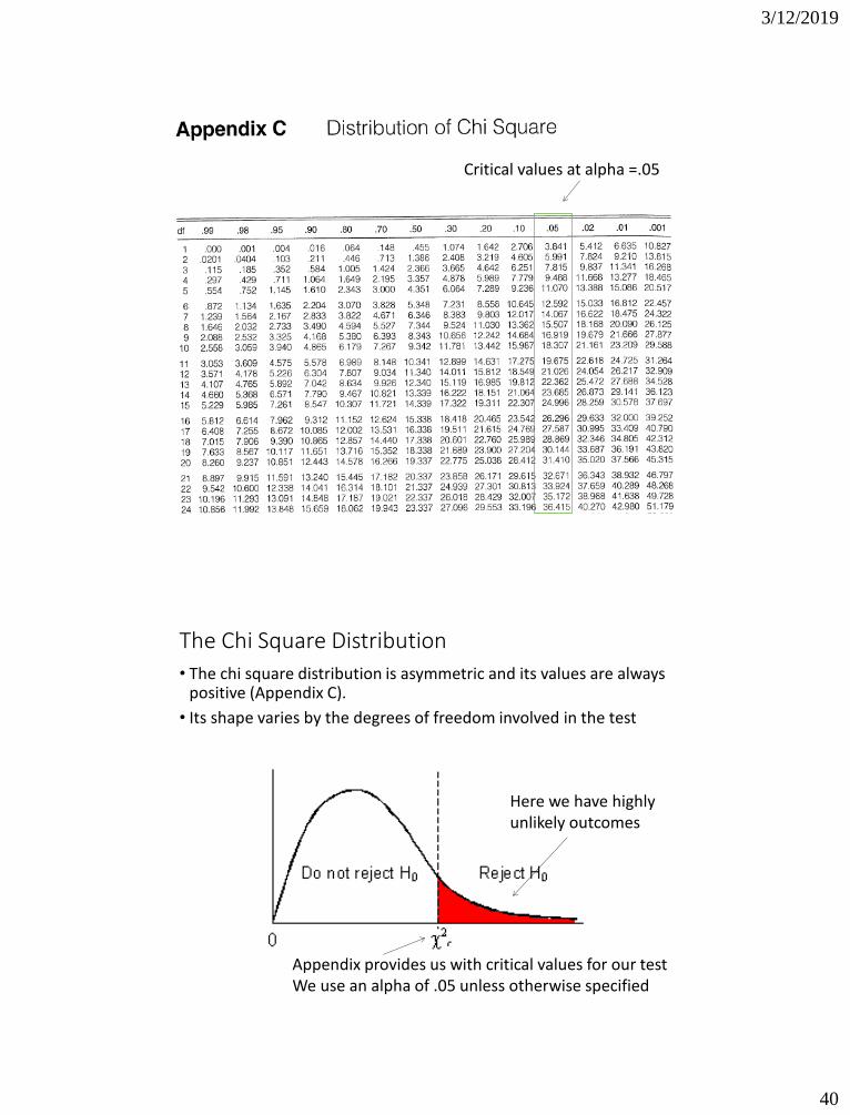
The Chi Square Distribution

• Type of sampling distribution

• The chi square distribution is asymmetric and its values are always positive (Appendix C).

• Its shape varies by the degrees of freedom involved in the test , which in turn is determined by the number of columns and rows in the table

• χ2 can be calculated for any bivariate table

• The shape of the χ2 distribution is influenced by the number of rows and columns in the table df=(r-1)(c-1)

• The sampling distribution we are working with in this case (TABLE C) relates to all possible χ2 under a hypothetical situation whereby we have independence with a table of given size (# of columns, # of rows)

• With our significance test, we work with this χ2 distribution (with the null hypothesis that we have “independence”), and determine whether our test statistic χ2 is likely or not,.. under this assumption

• If highly unlikely (we set our alpha at .05), we reject our null hypothesis, and conclude significance

• 95% confident that there is a relationship,.. If we set our alpha value at .05 and our test score falls within the critical area..

Working with the chi square distribution

3/12/2019

40

11-79

Critical values at alpha =.05

The Chi Square Distribution

• The chi square distribution is asymmetric and its values are always positive (Appendix C).

• Its shape varies by the degrees of freedom involved in the test

Appendix provides us with critical values for our test We use an alpha of .05 unless otherwise specified

Here we have highly unlikely outcomes

3/12/2019

41

• Is there a relationship between support for

privatization of healthcare and political ideology? Are

liberals significantly different from conservatives on

this variable? o The table below reports the relationship between these two variables

for a random sample of 78 adult Canadians.

Back to our example


11-82

• Independent random samples

• e.g. independent samples of conservatives & liberals

• Level of measurement is nominal

• e.g. support for privatization

Performing the Chi Square Test Using

the Five-Step Model

Step 1: Make Assumptions and Meet Test

Requirements

3/12/2019

42

11-83

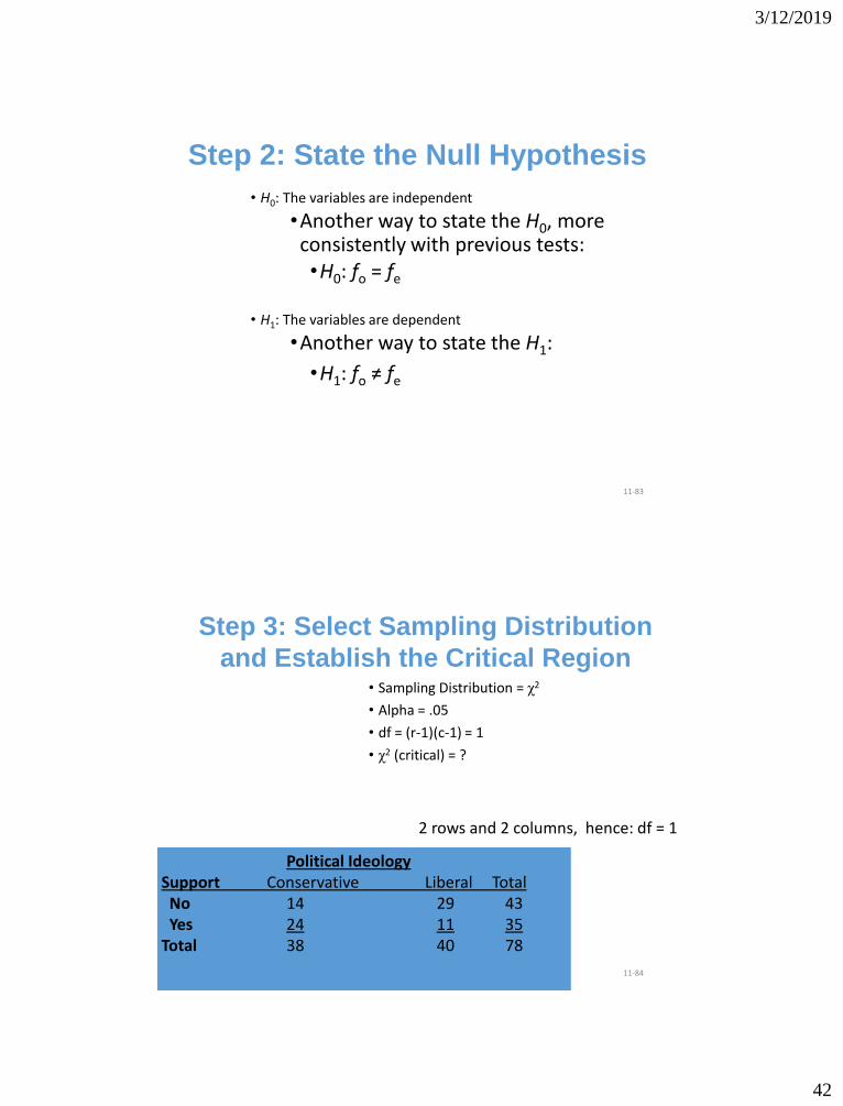
• H0: The variables are independent

•Another way to state the H0, more consistently with previous tests: •H0: fo = fe

• H1: The variables are dependent

•Another way to state the H1:

•H1: fo ≠ fe


11-84

• Sampling Distribution = χ2

• Alpha = .05

• df = (r-1)(c-1) = 1

• χ2 (critical) = ?

Step 3: Select Sampling Distribution

and Establish the Critical Region


2 rows and 2 columns, hence: df = 1

3/12/2019

43

11-85

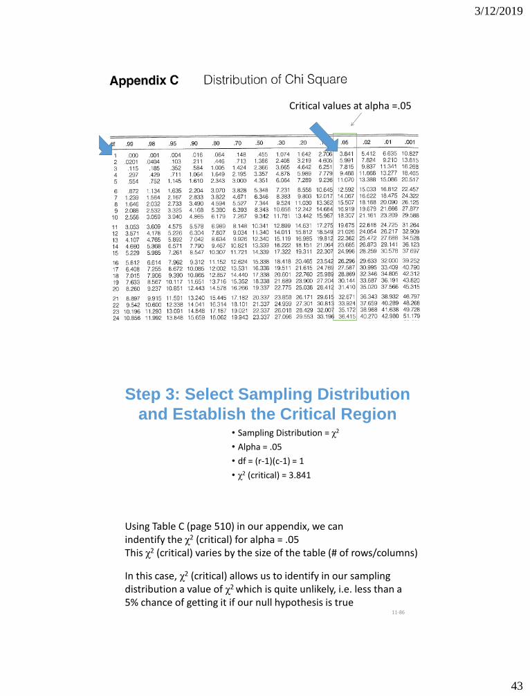
Critical values at alpha =.05

11-86

• Sampling Distribution = χ2

• Alpha = .05

• df = (r-1)(c-1) = 1

• χ2 (critical) = 3.841

Step 3: Select Sampling Distribution

and Establish the Critical Region

Using Table C (page 510) in our appendix, we can indentify the χ2 (critical) for alpha = .05 This χ2 (critical) varies by the size of the table (# of rows/columns)

In this case, χ2 (critical) allows us to identify in our sampling distribution a value of χ2 which is quite unlikely, i.e. less than a 5% chance of getting it if our null hypothesis is true

3/12/2019

44

11-87

Use Formula 10.2 to find fe.

– To obtain fe multiply column and row

marginals for each cell and divide by N. • (38*43)/78 = 1634 /78 = 20.9 • (40*43)/78 = 1720 /78 = 22.1 • (38*35)/78 = 1330 /78 = 17.1 • (40*35)/78 = 1400 /78 = 17.9

Expected frequencies (fe)

Political Ideology


No 20.9 22.1 43

Yes 17.1 17.9 35

Total 38 40 78

Step 4. Get our test statisitc (continued) Observed Frequencies (fo)

Conservative Liberal Total No 14 29 43 Yes 24 11 35 Total 38 40 78

11-88

Step 4: Calculate the Test

Statistic


2 /fe

14 20.9 -6.9 47.61 2.28

29 22.1 6.9 47.61 2.15

24 17.1 6.9 47.61 2.78

11 17.9 -6.9 47.61 2.66

78 78 0 χ2 = 9.87

As demonstrated earlier:

3/12/2019

45

11-89

• χ2 (obtained) = 9.87

Step 4: Calculate the Test

Statistic

11-90

• χ2 (critical) = 3.841

• χ2 (obtained) = 9.87

• The test statistic is in the Critical (shaded) Region:

– We reject the null hypothesis of independence. – Opinion on healthcare privatization is associated with political ideology.

Step 5: Make Decision and

Interpret Results

9.87

Documents

Chapter 9 Hypothesis Testing II - King's Facultydkerr.kingsfaculty.ca/dkerr/assets/File/StatsL92205.pdf · 2019. 3. 12. · 3/12/2019 10 9-19 The obtained test statistic (Z = 20)