Embed Size (px)
Citation preview
Copyright © 1998 IEEE. All rights reserved. 165
Chapter 7Short-circuit studies
7.1 Introduction and scope
Electrical power systems are, in general, fairly complex systems composed of a wide range of
equipment devoted to generating, transmitting, and distributing electrical power to various
consumption centers. The very complexity of these systems suggests that failures are
unavoidable, no matter how carefully these systems have been designed. The feasibility of
designing and operating a system with zero failure rate is, if not unrealistic, economically
unjustifiable. Within the context of short-circuit analysis, system failures manifest themselves
as insulation breakdowns that may lead to one of the following phenomena:
— Undesirable current flow patterns
— Appearance of currents of excessive magnitudes that could lead to equipment dam-
age and downtime
— Excessive overvoltages, of the transient and/or sustained nature, that compromise the
integrity and reliability of various insulated parts
— Voltage depressions in the vicinity of the fault that could adversely affect the opera-
tion of rotating equipment
— Creation of system conditions that could prove hazardous to personnel
Because short circuits cannot always be prevented, we can only attempt to mitigate and to a
certain extent contain their potentially damaging effects. One should, at first, aim to design
the system so that the likelihood of the occurrence of the short circuit becomes small. If a
short circuit occurs, however, mitigating its effects consists of a) managing the magnitude of
the undesirable fault currents, and b) isolating the smallest possible portion of the system
around the area of the mishap in order to retain service to the rest of the system. A significant
part of system protection is devoted to detecting short-circuit conditions in a reliable fashion.
Considerable capital investment is required in interrupting equipment at all voltage levels that
is capable of withstanding the fault currents and isolating the faulted area. It follows, there-
fore, that the main reasons for performing short-circuit studies are the following:
— Verification of the adequacy of existing interrupting equipment. The same type of
studies will form the basis for the selection of the interrupting equipment for system
planning purposes.
— Determination of the system protective device settings, which is done primarily by
quantities characterizing the system under fault conditions. These quantities also
referred to as “protection handles,” typically include phase and sequence currents or
voltages and rates of changes of system currents or voltages.
— Determination of the effects of the fault currents on various system components such
as cables, lines, busways, transformers, and reactors during the time the fault persists.
Thermal and mechanical stresses from the resulting fault currents should always be
compared with the corresponding short-term, usually first-cycle, withstand capabili-
ties of the system equipment.
IEEEStd 399-1997 CHAPTER 7
166 Copyright © 1998 IEEE. All rights reserved.
— Assessment of the effect that different kinds of short circuits of varying severity may
have on the overall system voltage profile. These studies will identify areas in the
system for which faults can result in unacceptably widespread voltage depressions.
— Conceptualization, design and refinement of system layout, neutral grounding, and
substation grounding.
Compliance with codes and regulations governing system design and operation, such as the
National Electrical Code® (NEC®) (NFPA 70-1996) [B6],1 article 110-9.
It is not the intention of this chapter to provide details on system modeling and computational
procedures under fault conditions, since these topics are exhaustively treated in many com-
prehensive textbooks and articles (see bibliography) and other IEEE publications such as
IEEE Std 141-1993,2 IEEE Std 241-1990, and IEEE Std 242-1986. Rather, the intention is to
address the subject of short-circuit analysis within the context of three-phase industrial and
commercial power systems by focusing on the following:
a) The concerns and fundamental phenomena associated with short-circuit studies
b) Viable computational approaches and some aspects of system modeling
c) Various factors affecting the results and accuracy of short-circuit studies
d) The salient principles, methodologies, and computational procedures suggested by
the North American IEEE and ANSI C37 standards, specifically, ANSI C37.06-1979,
ANSI C37.06-1987, IEEE Std C37.010-1979, IEEE Std C37.5-1979, and IEEE Std
C37.13-1990). Reference will, however, be made to the international standard, IEC
60909 (1988), because
1) It features several significant conceptual and computational deviations from the
C37 standards, and
2) Equipment designed and built according to European specifications is being sold
in North America, which should be analyzed on the equipment-tested ratings.
e) Computer-based solutions and related aspects of software dedicated to computerized
fault analysis
f) The outline of a typical short-circuit study procedure through an example
7.2 Extent and requirements of short-circuit studies
Short-circuit studies are as necessary for any power system as other fundamental system
studies such as power flow studies, transient stability studies, harmonic analysis studies, etc.
Short-circuit studies can be performed at the planning stage in order to help finalize the
system layout, determine voltage levels, and size cables, transformers, and conductors. For
existing systems, fault studies are necessary in the cases of added generation, installation of
extra rotating loads, system layout modifications, rearrangement of protection equipment,
verification of the adequacy of existing breakers, relocation of already acquired switchgear in
order to avoid unnecessary capital expenditures, etc. “Post-mortem” analysis may also
1The numbers in brackets correspond to those of the bibliography in 7.9.2Information on references can be found in 7.8.
IEEESHORT-CIRCUIT STUDIES Std 399-1997
Copyright © 1998 IEEE. All rights reserved. 167
involve short-circuit studies in order to duplicate the reasons and system conditions that led to
the system’s failure.
The requirements and extent of a short-circuit study will depend on the engineering objec-
tives sought. In fact, these objectives will dictate what type of short-circuit analysis is
required. The amount of data required will also depend on the extent and the nature of the
study. The great majority of short-circuit studies in industrial and commercial power systems
address one or more of the following four kinds of short circuits:
— Three-phase fault. May or may not involve ground. All three phases shorted together.
— Single line-to-ground fault. Any one, but only one, phase shorted to ground.
— Line-to-line fault. Any two phases shorted together.
— Double line-to-ground fault. Any two phases connected together and then to ground.
These types of short circuits are also referred to as “shunt faults,” since all four exhibit the
common attribute of being associated with fault currents and MVA flows diverted to paths
different from the prefault “series” ones.
Three-phase short circuits often turn out to be the most severe of all. It is thus customary to
perform only three phase-fault simulations when seeking maximum possible magnitudes of
fault currents. However, important exceptions do exist. For instance, single line-to-ground
short-circuit currents can exceed three-phase short-circuit current levels when they occur in
the vicinity of
— A solidly grounded synchronous machine
— The solidly grounded wye side of a delta-wye transformer of the three-phase core
(three-leg) design
— The grounded wye side of a delta-wye autotransformer
— The grounded wye, grounded wye, delta-tertiary, three-winding transformer
For systems where any one or more of the above conditions exist, it is advisable to perform a
single line-to-ground fault simulation. The fact that medium- and high-voltage circuit break-
ers have 15% higher interrupting capabilities for single line-to-ground faults should be taken
into account, if elevated single line-to-ground fault currents are found. Line-to-line or double
line-to-ground fault studies may also be required for protective device coordination require-
ments. It should be noted that, since only one phase of the line-to-ground fault can experience
higher interrupting requirements, the three-phase fault will still contain more energy because
all three phases will experience the same interrupting requirements.
Other types of fault conditions that may be of interest include the so-called “series faults”
(Anderson [B1]) and pertain to one of the following types of system unbalances:
— One line open. Any one of the three phases may be open.
— Two lines open. Any two of the three phases may be open.
— Unequal impedances. Unbalanced line impedance discontinuity.
IEEEStd 399-1997 CHAPTER 7
168 Copyright © 1998 IEEE. All rights reserved.
The term “series faults” is used because the above unbalances are associated with a redistri-
bution of the prefault load current. Series faults are of interest when assessing the effects of
snapped overhead phase wires, failures of cable joints, blown fuses, failure of breakers to
open all poles, inadvertent breaker energization across one or two poles and other situations
that result in the flow of unbalanced currents.
7.3 System modeling and computational techniques
7.3.1 AC and dc decrement
The basic physical phenomena that determine the magnitude and duration of the short-circuit
currents are
a) The behavior of the rotating machinery in the system
b) The electrical proximity of the rotating machinery to the short-circuit location
c) The fact that the prefault system currents cannot change instantaneously, due to the
significant system inductance
The first two can be conceptually linked to the ac decrement, while the third, to the dc
decrement.
7.3.1.1 AC decrement and rotating machinery
AC decrement is characterized by the fact that the magnetic flux trapped in the windings of
the rotating machinery cannot change instantaneously (constant flux theorem). This gradual
change is a function of the nature of the magnetic circuits involved. That is why synchronous
machines, under short-circuit conditions, feature different flux variation patterns as compared
to induction machines. The flux dynamics dictates that the short-circuit current decays with
time until a steady-state value is reached. Computationally convenient machine models,
widely used for short-circuit studies, picture rotating machines as constant voltages behind
time-varying impedances, as outlined in IEEE Std 141-1993 and IEEE Std 242-1986. For
modeling purposes, these impedances increase in magnitude from the minimum post fault
subtransient value X"d, to the relatively higher transient value X 'd, and finally reach the even
higher steady-state value Xd, assuming the fault persists long enough (in reality it is the volt-
age that decays). The rate of increase of machine reactances is different for synchronous gen-
erators/motors and induction motors, with the latter increasing more rapidly than the former.
This modeling framework is fundamental in properly determining the symmetrical rms val-
ues of the short-circuit currents furnished by the rotating equipment for a short circuit any-
where in the system.
7.3.1.2 DC decrement and system impedances
DC decrement is also characterized by the fact that because the prefault system current can-
not change instantaneously, a significant unidirectional component may be present in the fault
current depending on the exact instant of the occurrence of the short circuit (Anderson [B1],
Blackburn [B3], Roeper [B8], Stevenson [B10]). This unidirectional current component,
IEEESHORT-CIRCUIT STUDIES Std 399-1997
Copyright © 1998 IEEE. All rights reserved. 169
often referred to as dc offset, decays with time exponentially. The rate of decay is closely
related to the system reactances and resistances. Despite the fact that this decay is relatively
rapid, the dc component could last long enough to be sensed by the interrupting equipment,
particularly when rapid fault clearing is very desirable to maintain system stability or prevent
the damaging thermal and mechanical effects of the short-circuit currents. Total fault currents
interrupted by circuit breakers must take into account this unidirectional component, particu-
larly for shorter interrupting times as clearly outlined in IEEE Std C37.010-1979, IEEE Std
C37.13-1990, and IEEE Std C37.5-1979. The same component is equally important when
assessing the ability of a circuit breaker to close against or withstand short-circuit currents.
Fault currents containing high dc offsets, often present no zero crossings in the first few
cycles immediately after fault initiation and are particularly onerous to the circuit breakers of
large generators.
7.3.2 System modeling requirements
Industrial and commercial power systems are normally multimachine systems with many
motors and possibly more than one generator, all interconnected through transformers, lines,
and cables. There could also be one or more locations at which the local power system is
interconnected to a larger grid. These locations are commonly known as “utility-interface”
points. The objective of the short-circuit study is to properly determine the short-circuit cur-
rents and voltages at various system locations. In view of the dynamic nature of the short-
circuit current, it is essential to relate any calculated fault currents to a particular instant in
time from the onset of the short circuit. AC decrement analysis serves the purpose of cor-
rectly determining the symmetrical rms values of the fault currents, while dc decrement anal-
ysis will provide the necessary dc component of the fault current, thus yielding a correct
estimate of the total fault current. It is the total fault current which, in general, must be used
for breaker and switchgear rating and in some cases for protective device coordination. Sys-
tem topology considerations are equally important because the system layout and electrical
proximity of the rotating machinery to the fault location will determine the actual magnitude
of the short-circuit current. It therefore becomes necessary to devise a model for the system
as a whole and analyze it as such in a flexible, accurate, and computationally convenient
manner.
7.3.3 Three-phase vs. symmetrical components representation
It is customary for three-phase electrical systems to be represented on a single-phase basis.
This simplification, successfully employed for power flow and transient stability studies, rests
on the premise that the system is balanced or at least can be assumed to be so for practical
purposes (Anderson [B1], Blackburn [B3] Stevenson [B10], Wagner and Evans [B13]). Mod-
eling the system, however, on a single-phase basis is inadequate for analyzing phenomena
that involve serious system unbalances (Anderson [B1], Arrilaga, Arnold, and Harker [B2]).
Within the context of short-circuit analysis, only the three-phase shunt fault lends itself to
single-phase analysis, because the fault condition is balanced involving all three phases,
assuming a balanced three-phase system. Any other fault condition will introduce unbalances
that require including in the analysis the remaining two phases. There are two alternatives to
address the problem:
IEEEStd 399-1997 CHAPTER 7
170 Copyright © 1998 IEEE. All rights reserved.
a) Three-phase system representation. When the system is represented on a three-phase
basis, we explicitly retain the identity of all three phases. The advantage of three-
phase representation is that any kind of fault unbalance can be readily analyzed,
including simultaneous faults. Furthermore, the fault condition itself is specified with
somewhat greater flexibility, particularly for arcing faults. The main disadvantages of
the technique are the following:
1) It is not tractable for hand calculations, even for small systems.
2) Supposing that a suitable computer program is used, it can be data-intensive.
b) Symmetrical components representation. The symmetrical components analysis is a
technique that, instead of requiring analysis of the unbalanced system, allows for the
creation of three subsystems, the positive, the negative, and the zero-sequence sys-
tems, properly interconnected at the fault point, depending on the nature of the sys-
tem unbalance. Once modeled, the fault currents and voltages, anywhere in the
network, are then obtained by properly combining the results of the analysis of the
three-sequence networks (Anderson [B1], Blackburn [B3] Stevenson [B10], Wagner
and Evans [B13]). The distinct advantage of the symmetrical components approach is
that it allows modeling unbalanced fault conditions, while still retaining the concep-
tual simplicity of the single-phase analysis. Another important advantage of the sym-
metrical components method is that system equipment impedances can be easily
measured in the symmetrical components reference frame. This simplification is only
true if the system is balanced in all three phases (except at the fault location which
then becomes the interconnection point of the sequence networks), an assumption
that can be entertained without introducing significant modeling errors for most sys-
tems. The main disadvantage of the technique is that for complicated fault conditions,
it may introduce more problems than it solves. The symmetrical components tech-
nique remains the preferred analytical tool today for fault analysis for both hand and
computer-based calculations.
7.3.4 System impedances and symmetrical components analysis
The symmetrical components theory dictates that for a three-phase system, three sequence
systems need, in general, to be set up for the analysis of an unbalanced fault condition. The
first is the positive sequence system, which is defined by a balanced set of voltages and
currents, equal in magnitude, following the normal phase sequence of a, b, and c. The second
is the negative sequence system, which is similar to the positive sequence system, but is
defined by a balanced set of voltages and currents with a reverse phase sequence of a, c, and
b. Finally, the zero sequence system is a system defined by a set of voltages and currents that
are in phase with each other and not displaced by 120 degrees, as is the case with the other
two systems. The topology of the zero sequence system can be quite different from that of the
positive and negative sequence systems due to the fact that it depends heavily on the power
transformer connections (Anderson [B1], Blackburn [B3] Stevenson [B10]) and system neu-
tral grounding, factors which are not of importance when determining the topology of the
other two sequence networks.
Static system equipment like transformers, lines, cables, busways, and static loads present,
under balanced conditions, the same impedances to the flow of positive and negative
sequence currents. The same components present, in general, different impedances to the
IEEESHORT-CIRCUIT STUDIES Std 399-1997
Copyright © 1998 IEEE. All rights reserved. 171
flow of zero sequence currents. Rotating equipment like synchronous generators, motors,
condensers, and induction motors have different impedances in all three sequence networks.
The positive sequence impedances are the ones normally used for balanced power flow stud-
ies. All sequence impedances must be either calculated, measured, provided by the equipment
manufacturers, or estimated. The zero sequence impedance may not exist for some rotating
equipment, depending on the machine grounding.
For a balanced three-phase fault analysis, only the positive sequence system components
impedances Z1 (R1 + jX1) are required. For line-to-line faults, negative sequence impedances
Z2 (R2 + jX2) are also required. For all shunt faults involving ground, i.e., line-to-ground and
double line-to-ground, the zero sequence system impedances Z0 (R0 + jX0) are needed in
addition to the other two. System neutral grounding equipment data like grounding resistors,
reactors, transformers, etc., form an integral part of the zero sequence system impedance
data.
AC decrement considerations dictate that rotating equipment impedances vary from the onset
of the short circuit. This applies only to positive sequence impedances, which vary from sub-
transient through transient to steady-state values. The negative and zero sequence impedances
for the rotating equipment are considered unchanged. The same holds true for the impedances
of the static system equipment.
7.3.5 Computational approaches
7.3.5.1 Time domain fault analysis
Time-domain fault analysis pertains to techniques that allow for the calculation of the short-
circuit current as a function of time from the moment of the fault inception. For large electric
power systems, with many machines and generators contributing to the fault current, the con-
tributions of many machines will have to be taken into account concurrently. Machine models
have been developed that let predictions of considerable accuracy be made regarding the
behavior of any machine for a fault either at or beyond its terminals. These models are rather
complex because they tend to represent in detail not only the machine itself but also several
nonlinear controllers, such as excitation systems and their related stabilization circuitry, with
nonlinearities. It can therefore be seen that the calculating requirements could be stupendous,
because the problem is reduced to simultaneously solving a large number of differential equa-
tions. Despite its inherent power, the use of time-domain fault analysis is not very widespread
and is only used for special studies because it is data-intensive (data requirements can be at
least as demanding as transient stability analysis) and it requires special software.
7.3.5.2 Quasi-steady-state fault analysis
Quasi-steady-state fault analysis pertains to techniques that represent the system at steady
state. Phasors are used to represent system voltages, currents, and impedances at fundamental
frequency. System modeling and the resulting computational techniques are based on the
assumption that the system and its components can be represented by linear models.
Retaining linearity simplifies considerably the necessary calculations (Anderson [B1], Arril-
aga, Arnold, and Harker [B2], Blackburn [B3] Stevenson [B10], Wagner and Evans [B13]) as
IEEEStd 399-1997 CHAPTER 7
172 Copyright © 1998 IEEE. All rights reserved.
demonstrated in Chapter 3. Furthermore, linear algebra theory and the numerical advances in
matrix computations make it possible to implement very elegant computer solutions for
relatively large systems. These techniques have been favored by the various industry stan-
dards and will be briefly examined next.
7.4 Fault analysis according to industry standards
Industry standards dictate certain analytical techniques that adhere to specific guidelines,
suited to address the questions of ac and dc decrement in multimachine systems in
compliance with well-established, industry-accepted practices. They are also closely linked
to and harmonize quite well with existing switchgear rating structures. Typical standards are
the North American ANSI and IEEE C37 standards and recommended practices (see 7.4.1),
the international standard, IEC 60909 (1988) and others, such as the German VDE 0102-1972
and the Australian AS 3851-1991 (see 7.8). The analytical and computational framework in
the calculating procedures recommended by these standards remains algebraic and linear, and
the calculations are kept tractable by hand for small systems. The extent of the data base
requirements for computer-based solutions is carefully kept to a necessary maximum for the
results to be acceptably accurate. This type of analysis represents the best compromise
between solution accuracy and simulation simplicity. The great majority of commercial-
grade short-circuit analysis programs fall under this category.
In 7.4.1, an outline of ANSI and IEEE standards is presented, while in 7.4.2, the relevant
aspects of IEC 60909 (1988) are described. It is not the intent of these subclauses to fully
explore and describe in detail all pertinent clauses of either standard. Instead, a rather brief
summary is presented in an effort to make any potential user conscious of the salient aspects
of each technique. Because only a brief summary is presented, it is strongly recommended
that the standards be consulted for further clarifications and details.
7.4.1 The North American ANSI and IEEE standards
IEEE standards addressing fault calculations for medium and high voltage are IEEE Std
C37.010-1979, IEEE Std C37.5-1979, IEEE Std 141-1993, IEEE Std 241-1990, and IEEE
Std 242-1986. IEEE standards addressing fault calculations for low-voltage systems (below
1000 V), are the IEEE Std C37.13-1990, IEEE Std 141-1993, IEEE Std 241-1990, and IEEE
Std 242-1986. Three types of short-circuit currents are defined, depending on the time frame
of interest taken from the inception of the fault, as
a) First cycle currents
b) Interrupting currents
c) Time delayed currents
First-cycle currents, also called momentary currents, are the currents at 1/2 cycle after fault
initiation; they relate to the duty circuit breakers face when “closing against” or withstanding
short-circuit currents. That is why these currents are also called “close and latch” currents.
Often these currents contain dc offset, and they are calculated on the premise of no ac decre-
IEEESHORT-CIRCUIT STUDIES Std 399-1997
Copyright © 1998 IEEE. All rights reserved. 173
ment in the contributing sources (i.e., the machine reactances remain subtransient [see Table
7-1]). Since low-voltage breakers operate in the first cycle, their interrupting ratings are com-
pared to these currents.
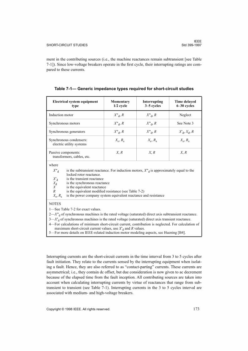
Interrupting currents are the short-circuit currents in the time interval from 3 to 5 cycles after
fault initiation. They relate to the currents sensed by the interrupting equipment when isolat-
ing a fault. Hence, they are also referred to as “contact-parting” currents. These currents are
asymmetrical; i.e., they contain dc offset, but due consideration is now given to ac decrement
because of the elapsed time from the fault inception. All contributing sources are taken into
account when calculating interrupting currents by virtue of reactances that range from sub-
transient to transient (see Table 7-1). Interrupting currents in the 3 to 5 cycles interval are
associated with medium- and high-voltage breakers.
Table 7-1— Generic impedance types required for short-circuit studies
Electrical system equipment type
Momentary1/2 cycle
Interrupting3–5 cycles
Time delayed6–30 cycles
Induction motor X"d, R X"d, R Neglect
Synchronous motors X"d, R X"d, R See Note 3
Synchronous generators X"d, R X"d, R X 'd, Xd, R
Synchronous condensers: electric utility systems
Xs, Rs Xs, Rs Xs, Rs
Passive components: transformers, cables, etc.
X, R X, R X, R
where
X"d is the subtransient reactance. For induction motors, X"d is approximately equal to the locked rotor reactance.
X 'd is the transient reactanceXd is the synchronous reactanceX is the equivalent reactanceR is the equivalent modified resistance (see Table 7-2)Xs, Rs is the power company system equivalent reactance and resistance
NOTES
1—See Table 7-2 for exact values.
2—X"d of synchronous machines is the rated voltage (saturated) direct axis subtransient reactance.
3—X 'd of synchronous machines is the rated voltage (saturated) direct axis transient reactance.
4—For calculations of minimum short-circuit current, contribution is neglected. For calculation ofmaximum short-circuit current values, use X 'd and R values.
5—For more details on IEEE-related induction motor modeling aspects, see Huening [B4].
IEEEStd 399-1997 CHAPTER 7
174 Copyright © 1998 IEEE. All rights reserved.
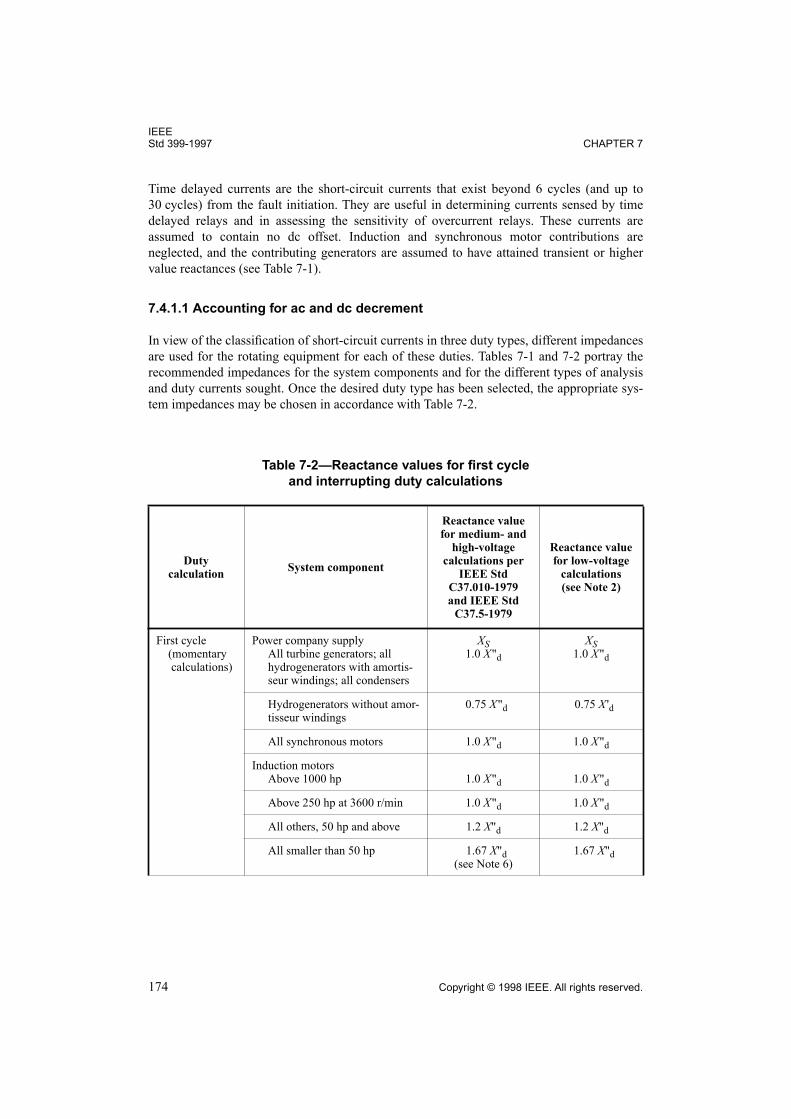
Time delayed currents are the short-circuit currents that exist beyond 6 cycles (and up to
30 cycles) from the fault initiation. They are useful in determining currents sensed by time
delayed relays and in assessing the sensitivity of overcurrent relays. These currents are
assumed to contain no dc offset. Induction and synchronous motor contributions are
neglected, and the contributing generators are assumed to have attained transient or higher
value reactances (see Table 7-1).
7.4.1.1 Accounting for ac and dc decrement
In view of the classification of short-circuit currents in three duty types, different impedances
are used for the rotating equipment for each of these duties. Tables 7-1 and 7-2 portray the
recommended impedances for the system components and for the different types of analysis
and duty currents sought. Once the desired duty type has been selected, the appropriate sys-
tem impedances may be chosen in accordance with Table 7-2.
Table 7-2—Reactance values for first cycle
and interrupting duty calculations
Dutycalculation
System component
Reactance value for medium- and
high-voltage calculations per
IEEE Std C37.010-1979and IEEE Std
C37.5-1979
Reactance value for low-voltage
calculations(see Note 2)
First cycle (momentary calculations)
Power company supplyAll turbine generators; all hydrogenerators with amortis-seur windings; all condensers
XS1.0 X"d
XS1.0 X"d
Hydrogenerators without amor-tisseur windings
0.75 X"d 0.75 X 'd
All synchronous motors 1.0 X"d 1.0 X"d
Induction motorsAbove 1000 hp 1.0 X"d 1.0 X"d
Above 250 hp at 3600 r/min 1.0 X"d 1.0 X"d
All others, 50 hp and above 1.2 X"d 1.2 X"d
All smaller than 50 hp 1.67 X"d(see Note 6)
1.67 X"d
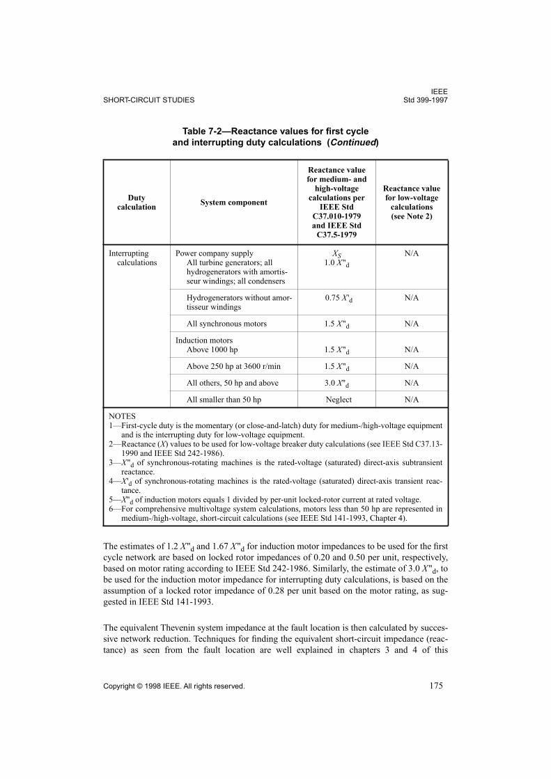
IEEESHORT-CIRCUIT STUDIES Std 399-1997
Copyright © 1998 IEEE. All rights reserved. 175
The estimates of 1.2 X"d and 1.67 X"d for induction motor impedances to be used for the first
cycle network are based on locked rotor impedances of 0.20 and 0.50 per unit, respectively,
based on motor rating according to IEEE Std 242-1986. Similarly, the estimate of 3.0 X"d, to
be used for the induction motor impedance for interrupting duty calculations, is based on the
assumption of a locked rotor impedance of 0.28 per unit based on the motor rating, as sug-
gested in IEEE Std 141-1993.
The equivalent Thevenin system impedance at the fault location is then calculated by succes-
sive network reduction. Techniques for finding the equivalent short-circuit impedance (reac-
tance) as seen from the fault location are well explained in chapters 3 and 4 of this
Interruptingcalculations
Power company supplyAll turbine generators; all hydrogenerators with amortis-seur windings; all condensers
XS1.0 X"d
N/A
Hydrogenerators without amor-tisseur windings
0.75 X 'd N/A
All synchronous motors 1.5 X"d N/A
Induction motorsAbove 1000 hp 1.5 X"d N/A
Above 250 hp at 3600 r/min 1.5 X"d N/A
All others, 50 hp and above 3.0 X"d N/A
All smaller than 50 hp Neglect N/A
NOTES1—First-cycle duty is the momentary (or close-and-latch) duty for medium-/high-voltage equipment
and is the interrupting duty for low-voltage equipment.2—Reactance (X) values to be used for low-voltage breaker duty calculations (see IEEE Std C37.13-
1990 and IEEE Std 242-1986).3—X"d of synchronous-rotating machines is the rated-voltage (saturated) direct-axis subtransient
reactance.4—X 'd of synchronous-rotating machines is the rated-voltage (saturated) direct-axis transient reac-
tance.5—X"d of induction motors equals 1 divided by per-unit locked-rotor current at rated voltage.6—For comprehensive multivoltage system calculations, motors less than 50 hp are represented in
medium-/high-voltage, short-circuit calculations (see IEEE Std 141-1993, Chapter 4).
Table 7-2—Reactance values for first cycle
and interrupting duty calculations (Continued)
Dutycalculation
System component
Reactance value for medium- and
high-voltage calculations per
IEEE Std C37.010-1979and IEEE Std
C37.5-1979
Reactance value for low-voltage
calculations(see Note 2)
IEEEStd 399-1997 CHAPTER 7
176 Copyright © 1998 IEEE. All rights reserved.
recommended practice, in IEEE Std 141-1993, in IEEE Std 241-1990, and in IEEE Std 242-
1986. The prefault system voltage, normally assumed to be 1.00 p.u. (rated), divided by the
equivalent short-circuit impedance, will yield the desired symmetrical rms value of the
desired three-phase fault current. The dc component of the fault current is obtained by con-
sidering the X/R ratio at the fault point. The X/R ratio is calculated by taking the ratio of the
system reactance (Thevenin equivalent reactance) to the system resistance (Thevenin equiva-
lent resistance) as seen from the fault location. The equivalent reactance must be calculated
from the reactance network (X) which is the impedance network of the system under study
with all resistances absent. Similarly, the equivalent resistance must be calculated from the
resistance network (R), which is the impedance network of the system under study with all
reactances absent.
It should be noted that the separate reactance and resistance network reduction technique will
yield a different X/R ratio (usually higher) than the phasor X/R ratio of the complex fault
impedances.
7.4.1.2 Calculated short-circuit currents and interrupting equipment
The calculating procedures briefly touched upon above are meant to address short-circuit
calculations on Industrial power systems with several voltage levels comprising high-,
medium-, and low-voltage circuits. First cycle currents are useful in calculating the interrupt-
ing requirements of low voltage fuses and breakers. Currents resulting from the same simula-
tion are effectively used in calculating the first-cycle requirements for medium- and high-
voltage fuses and circuit breakers. The currents resulting from the so-called interrupting net-
work calculations are only used for medium- and high-voltage circuit breakers, which operate
with a certain time delay due to relaying and operating requirements. It must be borne in
mind that since low-voltage fuse and circuit breaker application standards like IEEE Std
C37.13-1990 have adopted the symmetrical rating structure, calculating only the symmetrical
rms fault currents and the X/R ratio may be sufficient, if the calculated X/R ratio is less than
the X/R ratio of the circuit breaker test circuit.
A distinction has to be made between the various rating structures of medium- and high-
voltage circuit breakers. Breakers rated with the older rating structure, covered by IEEE Std
C37.5-1979, are assessed on the basis of the total asymmetrical fault current, or total prospec-
tive fault MVA, and calculations are normally restricted to minimum parting time for the sake
of safety and simplicity. The more recent rating structure, covered by IEEE Std C37.010-
1979, assumes breakers to be rated on a symmetrical basis. Depending on service conditions
and the system X/R ratio, the calculated symmetrical short-circuit currents may be sufficient,
because a certain degree of asymmetry is embedded in the breaker rating structure.
When calculation of the total fault current is warranted for medium- and high-voltage breaker
calculations, IEEE Std C37.010-1979 and IEEE Std C37.5-1979 contain tabulated multipliers
that can be applied to the symmetrical rms fault currents in order to obtain asymmetrical rms
currents. For IEEE Std C37.5-1979, these currents are the total asymmetrical fault currents,
whereas IEEE Std C37.010-1979 represents currents that are to be compared with the breaker
interrupting capabilities. In both cases, these multipliers are obtained from curves normalized
against breaker contact parting time. As of 1987, the ANSI C37.06-1987 introduced the peak
IEEESHORT-CIRCUIT STUDIES Std 399-1997
Copyright © 1998 IEEE. All rights reserved. 177
fault current to the preferred ratings as an alternative to the earlier total asymmetrical fault
currents (for first cycle withstand requirements) per ANSI C37.06-1979, in order to better
harmonize with IEC standards.
In summary, it should be stressed that an essential step for the calculation of the total fault
currents in medium- and high-voltage circuit breaker applications is the determination of por-
tions of the fault current coming from “local” and “remote” sources as a means of obtaining a
more reasonable estimate of the breaker interrupting requirements (Huening [B5]). The rea-
son for this distinction is that fault currents from remote sources feature slower, or no, ac cur-
rent decay as compared to currents coming from local sources. A “remote” contribution, as
defined in IEEE Std C37.010-1979, IEEE Std C37.5-1979, IEEE Std 141-1993, and IEEE Std
242-1986, is the fault current that comes from a generator that
a) Is located two or more transformations away from the fault, or
b) Has a per unit X"d that is 1.5 times less than the per unit external reactance on a com-
mon MVA basis.
Chapter 4 of IEEE Std 141-1993 provides details on the methods that can be used to deter-
mine the appropriate composite adjustment factors that account for local and remote short-
circuit contributions. The ratio of the remote source contributions to the total short-circuit
current is also known as the NACD ratio (Huening [B5]).
7.4.2 The international standard, IEC 60909 (1988)
IEC 60909 (1988) is similar to the German VDE 0102-1972 standard and to the Australian
AS 3851-1991 standard. In what follows, only the very salient aspects are discussed in an
effort to make the potential user conscious of its computational and modeling requirements. It
is strongly recommended that interested readers consult the standard itself for further details.
IEC 60909 (1988) recognizes four duty types that result in four calculated fault currents:
— The initial short-circuit current I"k
— The peak short-circuit current Ip
— The breaking short-circuit current Ib
— The steady-state fault current Ik
Although, the breaking and steady-state fault currents are conceptually similar to the inter-
rupting and time-delayed currents, respectively, the peak currents are the maximum currents
attained during the first cycle from a fault’s inception and are significantly different from the
first-cycle IEEE currents, which are total asymmetrical rms currents. The initial short-circuit
current is defined as the symmetrical rms current that would flow at the fault point if no
changes are introduced in the network impedances.
The IEC 60909 (1988) provides guidelines for calculating maximum and minimum fault cur-
rents. The former are to be used for breaker rating while the latter for protective device coor-
dination. The major governing factors in calculating maximum and minimum fault currents
IEEEStd 399-1997 CHAPTER 7
178 Copyright © 1998 IEEE. All rights reserved.
are the prefault voltages at the fault point and the fact that minimum fault currents are calcu-
lated with minimum connected plant.
The phenomenon of ac decrement is addressed by considering the actual contribution of
every source, depending on the voltage at its terminals during the short circuit. Induction
motor ac decrement is modeled differently than synchronous machinery decrement, because
an extra decrement factor representing the more rapid flux decay in induction motors is
included. AC decrement is only modeled when breaking currents are calculated.
The phenomenon of dc decrement is addressed in IEC 60909 (1988) by applying the princi-
ple of superposition for the contributing sources in conjunction with giving due regard to the
topology of the network and the relative locations of the contributing sources with respect to
the fault position. In addition, the standard dictates that different calculating procedures be
used when the contribution converges to a fault point via a meshed or radial path. These con-
siderations apply to the calculation of peak and asymmetrical breaking currents.
Steady-state fault currents are calculated by assuming that the fault currents contains no dc
component and that all induction motor contributions have decayed to zero. Synchronous
motors may also have to be taken into account. Furthermore, provisions are taken not only for
salient and round rotor synchronous machinery but, also for different excitation system
settings.
Prefault system loading conditions are of concern to IEC 60909 (1988) as well. In an attempt
to account for system loads leading to higher prefault voltages, the standard recommends that
prefault system voltages other than 1.00 per unit be used, without requiring a prefault load
flow solution. Furthermore, the standard recommends generator impedance correction factors
that may be applicable to their unit transformers as well.
7.4.3 Differences between the ANSI and IEEE C37 standards and IEC 60909
(1988)
The differences between the two standards are numerous and significant (Rodolakis [B7]).
Despite the conceptual association in the duty types, system modeling and computational
procedures are quite different in the two standards. That is why results calculated using both
standards can be quite dissimilar, with IEC 60909 (1988) having the tendency to yield higher
fault current magnitudes. The essential generic differences between the two standards can be
summarized in the following:
— AC decrement modeling in IEC 60909 (1988) is fault location-dependent and it quan-
tifies the rotating machinery’s proximity to the fault. The IEEE standard, on the other
hand, recommends universal, system-wide ac decrement modeling.
— DC decrement for IEC 60909 (1988) does not always rely on a single X/R ratio. In
general, more than one X/R ratio must taken into account. Furthermore, the notion of
separate X and R networks for obtaining the X/R ratio(s) at the fault point is not appli-
cable to IEC 60909 (1988).
— Steady-state fault current calculation in IEC 60909 (1988) takes into account syn-
chronous machinery excitation settings.
IEEESHORT-CIRCUIT STUDIES Std 399-1997
Copyright © 1998 IEEE. All rights reserved. 179
In view of these important differences, computer simulations adhering to the ANSI and IEEE
C37 standards cannot, in general, be used to cover the computational requirements of IEC
60909 (1988) and vice versa.
7.5 Factors affecting the accuracy of short-circuit studies
The accuracy of the calculated fault currents depends primarily on accurate modeling of the
system configuration and the system impedances used for the calculations. Other very impor-
tant factors include the correct modeling of system rotating load, connected generators, sys-
tem neutral grounding, and other system components and operating conditions.
7.5.1 System configuration
System configuration consists of the following:
a) The location of all the potential sources of fault current, i.e., synchronous generators,
synchronous motors, induction motors, and utility connection points, and
b) How these fault current sources are connected through transformers, lines, cables,
busways, and reactors.
It is conceivable that more than one single-line diagram should be considered for a given sys-
tem, depending on the system operating modes and on the nature of the study. If the study is
done to assess switchgear adequacy and/or selection, maximum fault currents should be cal-
culated. This entails that fault currents must be calculated under maximum rotating plant and
closed bus-ties (whenever applicable), while any utility interconnections should be assumed
to attain their highest fault levels. If the study is done to assess protection sensitivity require-
ments, some of these conditions may need to be relaxed. Different system service conditions
may force the study of more than one system topology alternative, particularly in protective
relaying studies.
7.5.2 System Impedances
AC and dc decrement modeling considerations are very important factors in properly select-
ing the impedances of the rotating equipment for short-circuit studies. It is important to con-
sult manufacturer’s catalogues, data sheets and, if necessary, to perform some calculations to
ascertain reliable impedance values. Typical values can be used in the absence of any other
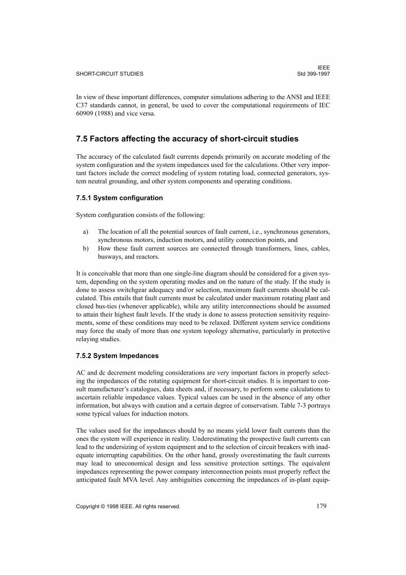
information, but always with caution and a certain degree of conservatism. Table 7-3 portrays
some typical values for induction motors.
The values used for the impedances should by no means yield lower fault currents than the
ones the system will experience in reality. Underestimating the prospective fault currents can
lead to the undersizing of system equipment and to the selection of circuit breakers with inad-
equate interrupting capabilities. On the other hand, grossly overestimating the fault currents
may lead to uneconomical design and less sensitive protection settings. The equivalent
impedances representing the power company interconnection points must properly reflect the
anticipated fault MVA level. Any ambiguities concerning the impedances of in-plant equip-
IEEEStd 399-1997 CHAPTER 7
180 Copyright © 1998 IEEE. All rights reserved.
ment should be resolved in favor of higher fault currents for the sake of safety in system
design. Impedances of bus ducts, busways, etc., must be accounted for in lower voltage cir-
cuits because they effectively limit fault current magnitudes. It is also customary practice to
use the saturated impedance values for synchronous machinery.
Last, but not least, the resistive components of the system impedances should be given proper
regard if operating system temperature is a factor or if significant lengths of cable runs are
present. Although resistance values can usually be omitted for fault current magnitude calcu-
lations (E/X calculation), they are important for calculating the system X/R ratio at the fault
point. Generally speaking, the total complex system impedance, Z (R+jX) has to be calculated
at the fault point to yield a more correct estimate of the fault current (E/Z calculation). This is
particularly true for low-voltage systems, where the system resistance is comparable in mag-
nitude to the system reactance and helps limit the fault current.
7.5.3 Neutral grounding
For faults necessitating the inclusion of zero sequence data, i.e., line-to-ground faults, double
line-to-ground shunt faults, and series faults, the flow of fault currents is appreciably affected
by the system grounding conditions. Of particular concern is the presence of multiple
grounding points and the values of system grounding impedances. Grounding impedances
can be used, to various degrees, to limit the value of the ground fault current to a minimum
value, to suppress resulting overvoltages, and to provide “handles” for ground protection.
System grounding can also play an important role in the proper simulation of the system zero
sequence response. More specifically, for solidly, or low-impedance grounded systems, it is
sufficient to include in the study only the occasional current limiting transformer and or gen-
Table 7-3—Typical values of motor impedances and kVA ratings
to use when exact values are not knowna
Induction motorSynchronous motor, 0.8 pfSynchronous motor, 1.0 pf
1 hp = 1 kVA1 hp = 1 kVA
.1 hp = 0.8 kVA
Motor type X"d (See Note)
Synchronous motors2–6 poles8–14 poles16 poles or more
0.150.200.28
Individual large induction motors, usually medium voltageAll others, 50 hp and aboveAll smaller than 50 hp, usually low voltage
0.670.670.67
NOTE—Motor impedances are in per unit on motor voltage and kVA rating. X"d for inductionmotors is approximately equal to the locked-rotor reactance. For induction motors, the locked-rotorreactance is the reciprocal value of the locked-rotor current. Reactances and motor base kVA ratingslisted were taken from data and assumptions in IEEE Std 141-1993.
aAs specified in IEEE Std 141-1993.
IEEESHORT-CIRCUIT STUDIES Std 399-1997
Copyright © 1998 IEEE. All rights reserved. 181
erator grounding impedances, while disregarding zero sequence line/cable charging shunts.
For high-impedance grounded, floating, and/or resonant-grounded systems, however, the lat-
ter will have to be taken into account (per IEC 60909 (1988), since the assumption that
neglecting it yields conservative (higher) fault currents is no longer valid.
7.5.4 Prefault system loads and shunts
It is customary to assume that the system is at steady state before a short circuit occurs. The
simplification of neglecting the prefault load is based on the premise that the magnitude of
the prefault system load current is, usually, much smaller than the fault current. The impor-
tance of the prefault load current in the system increases with rated system voltage and cer-
tain system loading patterns. That is why it is still justifiable for typical industrial power
system studies to assume a 1.00 per-unit prefault voltage for every bus. For systems in which
prefault loading is a concern, a prefault load flow analysis should precede the fault simula-
tions in order to ascertain a voltage profile for the system that will be consistent with the
existing system loads, shunts, and transformer tap settings. If the actual prefault system con-
dition is modeled, it is important to retain for the fault simulation all the system static loads
(normally neglected when the system is assumed at rest) as well as the capacitive line/cable
shunts.
Standards such as IEC 60909 (1988) and AS 3851-1991 attempt to address this issue by vir-
tue of using elevated prefault voltages and impedance correction factors for the synchronous
generators. The ANSI and IEEE C37 practice, however, is centered around considering the
prefault voltage as being the nominal system voltage with the notable exception being the
assessment of the interrupting requirements of circuit breakers.
7.5.5 Mutual coupling in zero sequence
This phenomenon is of importance when parallel circuits share the same right of way and
their geometrical arrangement is such that current flow in one circuit causes a voltage drop in
the other. A typical example is exposed overhead lines sharing the same support structure. It
should be noted that in reality, mutual coupling exists between phases in the positive
sequence as well. This form of mutual coupling, also known as “interphase coupling,” is not
explicitly modeled in positive sequence because it is restricted within the same circuit of
which only one phase is modeled. Zero sequence coupling, however, is extended between two
(or more) circuits and has to be explicitly modeled in zero sequence (Anderson [B1], Arril-
aga, Arnold, and Harker [B2], Blackburn [B3], Stagg and El-Abiad [B9], Wagner and Evans
[B13]). The implications of neglecting or incorrectly modeling this phenomenon leads to
erroneous calculation of ground fault currents and incorrect performance assessment of dis-
tance relays. Although relatively infrequent for industrial power system analysis, it should be
borne in mind and treated accordingly.
7.5.6 Phase shifts in delta wye transformer banks
When calculating the distribution of the three-phase fault current throughout a system, it is
often assumed that, going through transformer banks, the phase of the fault current from
IEEEStd 399-1997 CHAPTER 7
182 Copyright © 1998 IEEE. All rights reserved.
primary to secondary remains the same. This is true only if the transformer is connected wye-
wye or delta-delta. When a delta-wye transformer is involved, a phase shift is introduced
between the phase quantities of the primary and secondary. The phase shift is present in posi-
tive and negative sequence quantities only. Zero sequence quantities are not affected. North
American practice dictates that the positive sequence high side line-to-ground voltage must
lead the positive sequence low side line-to-ground voltage by 30 degrees. Earlier transformer
connections and phase labeling may not comply with that requirement (Wagner and Evans
[B13]). The same may also be true for transformers following overseas phasing standards.
The computational consequence of not accounting for this phase shift for unbalanced faults is
that different current magnitudes are obtained when going through a delta-wye bank because
the sequence currents are manipulated vectorially to obtain phase currents. This can lead to
inaccurate protective device settings which can, in turn, compromise the selectivity of an
overcurrent protection scheme (see also IEEE Std 141-1993 and IEEE Std 242-1986).
7.6 Computer solutions
7.6.1 General
Short-circuit calculations are generally less computationally intensive than other basic power
system studies like power flow or harmonic analysis. In view of the fact that short-circuit cal-
culations are linear systems of small to medium sizes can be computationally tractable by
hand, particularly if the system resistances are neglected to avoid complex arithmetic. Calcu-
lations are further simplified for radial systems. Practical industrial systems, however, can
contain several hundred to over one thousand buses, particularly if representation of low-
voltage circuits, smaller rotating loads and protective gear is warranted. Under these condi-
tions, computer solutions are the only practical alternative. It should be noted, however, that
the speed and reliability of computer-based calculations are rapidly rendering hand-calcula-
tions a rarity even for small systems.
7.6.2 Computerized network solutions: System matrices
Hand calculations for determining the equivalent system impedance at a fault point rely on
successive and judiciously chosen combinations of the system branches, until the system is
reduced to an equivalent Thevenin impedance. This has to be repeated for every new fault
location. Since this is done by inspecting the network, the intuition of the analyst is essential.
Computers do not have any intuition, that is why different techniques are used. These tech-
niques do not rely on the analyst’s inspection abilities, nor do they assume any system topol-
ogy. That is why they lend themselves very well to both radial and looped systems and are
capable of accommodating systems of practically any size. The notions of admittance and
impedance matrices are central in realizing any computerized solution scheme.
7.6.2.1 The bus admittance matrix
The bus admittance matrix, also called the Y-matrix, is a square complex matrix (a matrix
whose entries are complex numbers) with as many rows and columns as the system buses
IEEESHORT-CIRCUIT STUDIES Std 399-1997
Copyright © 1998 IEEE. All rights reserved. 183
(Anderson [B1], Arrilaga, Arnold, and Harker [B2], Stevenson [B10], Stagg and El-Abiad
[B9]). The elements of this matrix are either component admittances or sums of component
admittances. The term “component admittance” denotes the inverse of the component com-
plex impedance with a component being a system branch, generator, motor, etc. Once the
system buses have been identified, this matrix can be constructed as follows:
— Assign a diagonal matrix element to every system bus. The value of the matrix diago-
nal elements is the sum of the admittances of all the power system components con-
nected to that bus.
— Assign a nondiagonal element to all the matrix elements that represent a system
branch. For instance, if a branch is connected between buses i and j, the matrix entry
Yij will be nonzero and equal to the negative sum of the admittances of all compo-
nents directly connected between buses i and j.
Electric power systems are passive and have very few branches compared to all of the possi-
ble bus connections, and as a result, typical power system bus admittance matrices are
a) symmetric (assuming that transformers are not modeled in off-nominal tap positions)
which means that Yij = Yji, and
b) sparse, i.e., they feature a lot of zero entries.
7.6.2.2 The bus impedance matrix
The bus impedance matrix, also called the Z-matrix, is defined as the inverse of the admit-
tance matrix (Anderson [B1], Arrilaga, Arnold, and Harker [B2], Stevenson [B10], Stagg and
El-Abiad [B9]). This complex matrix is also square and symmetric, i.e., the entry Zij equals
the entry Zji, for passive networks. As the inverse of the sparse Y-matrix, however, this matrix
is a full matrix having no zero entries. It can be proved that the diagonal entries, Zii for bus i,
of this matrix are the equivalent Thevenin impedances used for fault calculations. The entry
Zij, however, does not necessarily represent the value of the impedance of the physical con-
nection between buses i and j. In fact, there is always an impedance Zij despite the fact that
there may not be a branch between buses i and j. The diagonal entries of the Z-matrix are used
in calculating fault currents, while the nondiagonal entries are useful for calculating branch
contributions and system-wide voltage profiles under fault conditions.
7.6.2.3 System topology, matrix sparsity, and solution algorithms
The sparsity of the Y-matrix requires that special techniques be employed for storing the sys-
tem data, because conceptually straightforward storage techniques may be quite wasteful.
Storing, for instance, the entire Z-matrix is not only impractical but unnecessary because only
a few of its elements may be needed. The development of solution algorithms, therefore, has
been focusing on the efficient retrieval of the necessary Z-matrix entries with the smallest
possible storage and calculation requirements. Modern vintage computer software employs
calculation and system data storage schemes that center around the so-called “sparse vector”
and/or “sparse matrix” solution techniques (Tinney, Brandwajn, Chan [B12]) which render
very rapid and accurate solutions.
IEEEStd 399-1997 CHAPTER 7
184 Copyright © 1998 IEEE. All rights reserved.
7.6.3 Computer software
7.6.3.1 General
The availability of commercial grade computer software on personal computers has been
steadily increasing in variety and computational power since the early 1980s, although
sophisticated software has existed for more powerful hardware platforms such as mainframes
and minicomputers since the early 1960s (St. Pierre [B11]). The personal computer is now
recognized as a credible computational tool due to the significant advances it has enjoyed in
processor architecture, speed, memory capacity, and in user-friendly operating systems and
environments. Computer programs that addressed short-circuit calculations were among the
first to be developed in all platforms. All programs rely on matrix techniques and require the
analyst to provide accurate system data so that the computer can proceed with the analysis
and produce the results.
7.6.3.2 Selecting software
The great variety of commercially available computer programs for short-circuit calculations
can be attributed to the wide variety of the analytical tasks they perform, the degree of sophis-
tication in user-interface and user-friendliness, and the computer platform for which they are
designed. Because the variety of the available computer software is accompanied by an
equally impressive variation in prices, it is important to acquire software that best corre-
sponds to the bulk of the engineering mandates for which it is purchased. It is questionable,
from an investment point of view, to acquire expensive and very sophisticated software when
the bulk of its analytical features will never be used. On the other hand, it could prove short-
sighted to acquire inexpensive software that will rapidly be outgrown by the needs of its user,
compromise the accuracy of the study, or result in a consistent waste of time and resources
due to inherent functional inefficacies. It is also important to assess the degree of user-friend-
liness of the software versus the computer-literacy of the personnel who will be using it.
Many engineers are reluctant to refamiliarize themselves with bulky user’s guides only to
perform studies with which they are very familiar. It pays to work with software that features
easy data entry, meaningful and helpful diagnostic messages, and comprehensive reports.
Last, it is essential to acquire software that is very well documented, promptly supported, and
regularly updated and upgraded by its vendors.
7.6.3.3 Features of short-circuit analysis software
The previously mentioned general salient principles governing software selection are supple-
mented by a good number of other features that are particularly applicable to short-circuit
analysis. A very important aspect in short-circuit studies is data preparation, a stage which,
by itself, can be computationally demanding, particularly if the software accepts system data
only on a per-unit basis. It is essential for the program to help the analyst prepare the data for
the study and provide means of identifying and correcting obvious and common mistakes.
Furthermore, whenever international standards are to be used, it is important for the software
to provide sufficient information and results that are transparent enough to allow for more
than one interpretation.
IEEESHORT-CIRCUIT STUDIES Std 399-1997
Copyright © 1998 IEEE. All rights reserved. 185
Table 7-4 contains several features that computer programs may or may not support. These
features have been conceptually categorized as “very desirable,” “desirable,” and “optional.”
“Very desirable” means that the feature is widely encountered and rather indispensable. The
category “desirable” addresses features that will prove of value to more demanding studies.
The category “optional” covers features that may prove to be of value for special studies.
Table 7-4—Analytical features of short-circuit computer programs
Analytical featureVery
desirable Desirable Optional
Systems with more than one voltage level Yes
Looped and radial system topology Yes
Ground faults (LG and LLG) Yes
Series faults (See Note 1) Yes
Arcing faults (See Note 2) Yes
Simultaneous faults Yes
Complex arithmetic Yes
Explicit negative sequence (See Note 3) Yes
Interface with power flow (See Note 1) Yes
Currents in all three phases (See Note 4) Yes
Currents in all three sequences (See Note 4) Yes
One-bus-away fault contributions Yes
Line monitors (See Note 5) Yes
Input data reports Yes
Protection coordination interface Yes
Voltages in nonfaulted buses (See Note 5) Yes
Summary reports Yes
Currents in all branches (See Note 5) Yes
Per-unitization of equipment data Yes
Rotating equipment impedance adjustment(IEEE Std C37.010-1979)
Yes
Separate X and R reduction for X/R ratios (IEEE Std C37.010-1979)
Mandatory
IEEEStd 399-1997 CHAPTER 7
186 Copyright © 1998 IEEE. All rights reserved.
Remote and local fault contributions(IEEE Std C37.010-1979)
Mandatory
First cycle fault currents (IEEE Std C37.010-1979) Mandatory
Interrupting fault currents (IEEE Std C37.010-1979) Mandatory
Time-delay fault currents (IEEE Std C37.010-1979) Yes
Symmetrical current multiplying factors(IEEE Std C37.010-1979)
Yes
Total current multiplying factors(IEEE Std C37.5-1979 factors)
Yes
Multiplying factors (IEEE Std C37.13-1990) Yes
X/R—dependent 1/2 cycle multipliers(IEEE Std C37.010-1979)
Yes
X/R—dependent peak multipliers(IEEE Std C37.010-1979)
Yes
Transformer phase shifts (See Note 4) Yes
Mutual coupling in zero sequence (See Note 6) Yes
Methodology in accordance with IEC 60909 (1988) (See Note 7)
Yes
NOTES1—Series faults are normally modeled when a prefault power flow solution is available and prefault
load can be taken into account.2—Arcing faults can be of consequence when assessing the sensitivity of ground protection in solidly
grounded systems. Conservative estimates of fault levels, however, will result by assuming boltedfaults.
3—Negative sequence system representation is not warranted by ANSI and IEEE C37 standards,though it could be of significance when ground faults near large generating stations are calculat-ed, or when simulations compatible with IEC 60909 (1988) require elevated accuracy.
4—It is important to have a good estimate of all three phase and sequence currents, particularly forprotection requirements. In correctly estimating all these currents in magnitude and phase it isvery helpful to take into account phase shifts in transformer banks.
5—When assessing the degree of severity of a fault, it is often of interest to see how nearby systemareas are affected, and if protective devices will be activated as a result of the fault.
6—Mutual coupling in zero sequence normally affects overhead circuitry sharing a common right-of-way. For industrial power systems analysis, zero sequence mutual coupling can be of concernif such circuits are modeled and the performance of protective devices requiring zero sequencecurrent compensation is investigated.
7—Support of the IEC 60909 (1988) may require dedicated software.
Table 7-4—Analytical features of short-circuit computer programs (Continued)
Analytical featureVery
desirable Desirable Optional
IEEESHORT-CIRCUIT STUDIES Std 399-1997
Copyright © 1998 IEEE. All rights reserved. 187
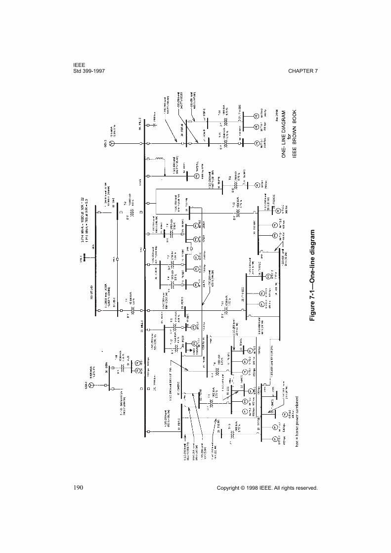
7.7 Example
In what follows, a short-circuit study is carried on a typical industrial system in order to illus-
trate typical steps, calculation requirements, and results. The system is composed of circuits
of several voltage levels, local generation, a utility interconnection, and a variety of rotating
loads. The study is carried out according to the ANSI and IEEE C37 standards (see 7.8).
7.7.1 Determination of the scope and extent of the study
Determination of the scope extent and the desired accuracy of the study is crucial, because
these factors will dictate what types of faults are to be simulated and to what degree system
modeling is to be undertaken. The type and number of fault studies for a given system is
determined by engineering judgment, which is based on the various forms the system layout
may assume during operation or the specific purpose of the study.
The study results may be used for recommending changes to existing plants or for proposing
an initial design for a system in its planning and/or expansion stage. Some important ques-
tions for which fault studies may help provide answers are as follows:
a) Is circuit interrupting equipment adequate for the system interrupting requirements at
all voltage levels? Can the medium- and high-voltage switchgear withstand the
momentary and interrupting duties imposed by the system? Is this switchgear ade-
quate for line to ground faults? If not, should new equipment be purchased or can
some changes to the system be effected to avoid the extra capital expenditure?
b) Is there any reserve in the interrupting capability of the circuit breakers for accommo-
dating future system expansion? If not, is it necessary to have a safety margin for
future expansion? If so, how can the system be changed to accommodate these con-
cerns?
c) Is noninterrupting equipment, i.e., reactors, cables, transformers, bus ducts, ade-
quately rated to withstand short-circuit currents until cleared by the interrupting
equipment?
d) Do load circuit breakers or disconnecting switches have sufficient momentary brac-
ing and/or close-and-latch capabilities?
e) What will be the effect on the calculated short-circuit currents in the plant system if
there is an increase in the power company’s short-circuit level? Economically, what
can be done to anticipate such an eventuality?
f) Is special protective equipment or circuitry necessary to provide protective device
selectivity for both maximum and minimum value of short-circuit currents?
g) During faults, do the voltages on unfaulted buses in the system drop to levels that can
cause motor-starter contactors to drop out or undervoltage relays to operate?
Every study will have to be assessed on its own merits and its results interpreted only for the
purpose the study was conducted. The short-circuit study for the example in question is per-
formed for the purposes of determining the interrupting requirements for low-, medium-, and
high-voltage switchgear. It is not uncommon for these types of studies to consider only three-
phase fault currents, since, as a rule, they yield the more severe interrupting requirements, as
compared to other shunt faults, and the industrial power systems are often impedance-
IEEEStd 399-1997 CHAPTER 7
188 Copyright © 1998 IEEE. All rights reserved.
grounded. Line-to-ground fault simulations are necessary for circuit-breaker-adequacy evalu-
ation and/or selection, if the system is such that line-to-ground fault currents may exceed
three-phase fault currents (see 7.2). Only three-phase, bolted, shunt faults will be considered
for the example.
7.7.2 Preparation of the system one-line diagram and collection of data
The one-line diagram of the system is shown in Figure 7-1. We will consider that both in-
plant generators are connected and that both of the utility service entrance transformers are in
service. The system rotating load, as shown in the one line diagram, represents an operating
condition that is typical for the system operating at or near full capacity. Furthermore, it is
known that the bus ties between buses 3 and 4 (13.8 kV) and between buses 1 and 2 (69 kV)
are open. Cable runs between buses, 9 (FDR E) and 13 (T6 PRI), 28 (T10 SEC) and 38 (480
TIE), 30 (T12 SEC) and 38 (480 TIE), 10 (EMER) and 12 (T5 PRI), are also assumed to be
open. It is this particular system layout that will be studied. In general, however, depending
on the type of study, more than one single-line diagram may have to be considered in practice
(see 7.5.1).
Data necessary for conducting a short-circuit study comprise the following:
a) Utility interconnection points and associated fault MVA levels (both three-phase and
line-to-ground) in order to determine the equivalent impedance of the utility
b) In-plant generation data
c) Rotating load data comprising synchronous motors and induction motors, both stand-
alone and grouped
d) Static system equipment data, such as transformers, cables, reactors, overhead lines,
busways, bus ducts, etc., switching equipment and, in some cases, static loads (heat-
ers, drives, etc.).
7.7.3 Determination and per-unitization of system impedances
7.7.3.1 Determination of the required system impedances
The choice of system impedances to be used depends on the type of study to be performed
and the actual fault conditions to be simulated. Three-phase fault studies require only positive
sequence impedances, whereas faults involving ground will require zero sequence system
data as well as any neutral grounding data. Negative sequence impedances may also be neces-
sary for line-to-line fault simulations. Impedances of both static and rotating system compo-
nents are normally known from equipment nameplate data. In the absence of detailed
information, typical values are assumed. Nameplate impedances of rotating equipment are
modified from their rated values in order to account for ac decay, according to the North
American practice (see 7.4.1).
7.7.3.2 Per-unitization of the system impedances
Power system equipment impedances are expressed on a unified per-unit basis because
IEEESHORT-CIRCUIT STUDIES Std 399-1997
Copyright © 1998 IEEE. All rights reserved. 189
a) Carrying out the calculations in ohms is not practical for systems composed of more
than one voltage level, and
b) The impedances of the system components are expressed in terms of their rated volt-
age and power.
When the per-unitization of the system impedances to a common MVA base is done manu-
ally, caution is required because this is a common source of errors. It is also one of the most
time-consuming tasks of a short-circuit study. Computer programs, in general, operate inter-
nally on per-unitized impedances, and many offer the facility to convert the “raw” system
data to per-unit data in a form ready to be used by the program. If this is the case, it is impor-
tant to comprehend how the per unitization is carried out. This will greatly facilitate any
future “what if” analysis because of different system layouts or modified system impedances.
In any case, any error in per unitizing the system impedances can seriously compromise the
accuracy of the short-circuit study.
Per-unit impedances are defined as the ratio of the actual ohmic component impedances to a
certain base impedance (see also Chapters 3 and 4). The base impedances are calculated from
a common, arbitrarily chosen, apparent power base and from a base voltage (Anderson [B1],
Stevenson [B10]).
(7-1)
The power base is usually expressed in MVA and is applicable throughout the system. The
base voltage is expressed in kilovolts (if base power is in MVA) and selected differently for
every system section, following the nominal voltage ratios of the system power transformers.
If single phase power is chosen, line-to-ground voltages should be used. Alternatively, if three
phase power is chosen as base line to line voltages are in order. It is practical to select as base
voltages the rated transformer voltages. All buses in the same network section must share the
same voltage base. Equipment like transformers, generators, motors, etc., have their imped-
ances given in percent (per unit × 100) of their rated voltage and power. It is often necessary
to convert these impedances to new base quantities as follows:
(7-2)
In what follows, some per-unit impedances used in the example study are calculated.
7.7.3.3 Power company per-unit impedance
Assuming that the three-phase MVA fault level at bus 100-UTIL-69 is 1000 MVA, the per-
unit impedance of the power company, for a 10 MVA base for the system, is calculated to be
(7-3)
Zp.u.
Zohms
Zbase
------------- with Zbase ,V base
2
Sbase
-----------= =
Zp.u., new
Snew
Sold
----------V old
2
V new
2----------- Zp.u., old=
Zutility
MVAbase
MVAfault
---------------------10
1000------------ 0.01 p.u.= = =
IEEEStd 399-1997 CHAPTER 7
190 Copyright © 1998 IEEE. All rights reserved.
Fig
ure
7-1
—O
ne-l
ine d
iag
ram
IEEESHORT-CIRCUIT STUDIES Std 399-1997
Copyright © 1998 IEEE. All rights reserved. 191
Assuming a typical X/R ratio of 22.0, the utility equivalent impedance becomes
This impedance will be applied for both first cycle and interrupting duty calculations because
the power company is considered always to be a “remote” source, thus featuring no ac
decrement.
7.7.3.4 Power cable per-unit impedance
Power cable impedances are normally provided in
Ω/1000 ft. Consider, as an example, the
cable connecting buses 3-MILL-1 and 9-FDRE, which is a 250MCM, 3-core, copper conduc-
tor, PVC-jacketed cable, and applied at 13.8 kV. The impedance of the cable is Z = 0.0440419
+ j0.0366795
Ω/1000 ft. The cable conduit between the two buses spans 650 ft. The imped-
ance of this cable expressed in per unit of system data will be
This impedance, as with all impedances of power cables and overhead circuitry, will be
applied as is for both first cycle and interrupting calculations. Impedance correction decre-
ment factors apply only to rotating induction and synchronous loads and in some cases to
synchronous generators (see Table 7-2).
7.7.3.5 Synchronous generator per-unit impedance
The generator connected on bus 4-MILL-2 has a rated power of 12.5 MVA, a rated voltage of
13.8 kV, a subtransient reactance of 12.8%, and an X/R ratio of 35.7. The reactance of the
generator on the common system MVA base of 10 MVA is found to be
The generator impedance, for the given X/R ratio, therefore becomes
For the example at hand, it will be assumed that all generators are turbo generators, thus
ac decrement impedance correction factors will be equal to 1.00 for interrupting duty
calculations.
Z2
R2 X
2
R2
------R2
+ R2
1.0X
2
R2
------+
from which ,= =
Zutility 0.000454 j0.00999 p.u.+=
Zcable p.u. 0.650 0.0440419 j0.0366795+ ( )10.00
13.82
------------- 0.0015032 j0.0012519 p.u.+= =
Xp.u., new
MVAnew
MVAold
---------------------V old
2
V new
2-----------
13.82
13.82
------------0.128 0.1024 p.u.= =
Zp.u.
0.1024
35.7---------------- j0.1024+ 0.002868 j0.1024 p.u.+= =
IEEEStd 399-1997 CHAPTER 7
192 Copyright © 1998 IEEE. All rights reserved.
7.7.3.6 Synchronous motor per-unit impedance
Consider the synchronous motor connected at bus 8-FDR-L. This motor has a subtransient
reactance of 20.00%, an X/R ratio of 34.00, and is rated 9000 kVA at 13.8 kV. The motor
impedance, expressed on a 10 MVA, 13.8 kV base reference, will then be
The impedance calculated for the synchronous motor is applicable to both first cycle and
interrupting calculations (see Table 7-2).
7.7.3.7 Induction motor per-unit impedances
7.7.3.7.1 Small induction motors
The motor load at bus 51-AUX partly consists of many small motors rated below 50 hp, total-
ing 570 hp, connected at 480 V, rotating at 1800 r/min. Assuming a total equivalent locked
rotor reactance of 16.7% and an X/R ratio of 12.00, the per-unit impedance of the group of
motors becomes
Alternative interpretations of IEEE Std C37.010-1979 and IEEE Std C37.13-1990, governing
first-cycle duty calculations, recommend omitting these motors for medium- and high-volt-
age, while considering them for low-voltage calculations. By applying the factor 1.67, both
high- and how-voltage circuits are modeled in one network and a single computer simulation
will suffice. For medium- and high-voltage interrupting duty calculations, these motors are
neglected (see Table 7-2).
7.7.3.7.2 Medium-sized induction motors
The motor load at bus 51-AUX also comprises a medium-sized induction motor, rotating at
1800 r/min, rated 200 kVA (200 hp with 0.746 power factor) at 480 V, with a locked rotor
reactance of 16.7% and an X/R ratio of 7.00. According to Table 7-2, the per-unit motor
impedances to be used in first cycle (impedance adjustment factor of 1.2) and interrupting
duty (impedance adjustment factor of 3.0) calculations are
Z syn p.u.
0.20
3.40---------- j0.20+
10.00
9.000-------------
13.82
13.82
------------ 0.006534 j0.2222 p.u.+= =
Zp.u.
0.167
12.00------------- j0.167+
10.00
0.570-------------
0.482
0.482
------------ 1.67 0.40773 j4.89278 p.u.+= =
Z first cycle p.u.
0.167
7.00------------- j0.167+
10.00
0.200-------------
0.482
0.482
------------ 1.20 1.43143 j10.0200 p.u.+= =
Z inter. p.u.
0.167
7.00------------- j0.167+
10.00
0.200-------------
0.482
0.482
------------ 3.00 3.57858 j25.0500 p.u.+= =
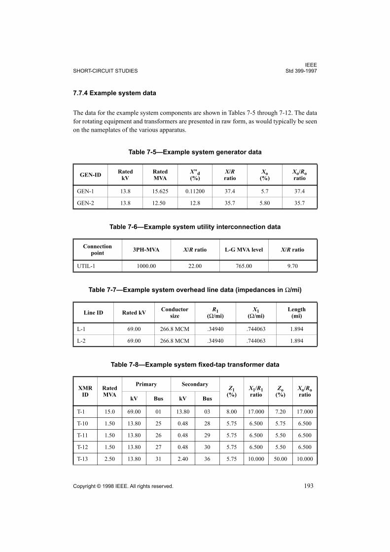
IEEESHORT-CIRCUIT STUDIES Std 399-1997
Copyright © 1998 IEEE. All rights reserved. 193
7.7.4 Example system data
The data for the example system components are shown in Tables 7-5 through 7-12. The data
for rotating equipment and transformers are presented in raw form, as would typically be seen
on the nameplates of the various apparatus.
Table 7-5—Example system generator data
GEN-IDRated
kVRatedMVA
X"d(%)
X/Rratio
Xo(%)
Xo/Roratio
GEN-1 13.8 15.625 0.11200 37.4 5.70 37.4
GEN-2 13.8 12.500 12.8 35.7 5.80 35.7
Table 7-6—Example system utility interconnection data
Connectionpoint
3PH-MVA X/R ratio L-G MVA level X/R ratio
UTIL-1 1000.00 22.00 765.00 9.70
Table 7-7—Example system overhead line data (impedances in
Ω/mi)
Line ID Rated kVConductor
sizeR1
(
Ω/mi)X1
(
Ω/mi)Length
(mi)
L-1 69.00 266.8 MCM .34940 .744063 1.894
L-2 69.00 266.8 MCM .34940 .744063 1.894
Table 7-8—Example system fixed-tap transformer data
XMRID
RatedMVA
Primary SecondaryZ1
(%)X1/R1ratio
Zo(%)
Xo/Roratio
kV Bus kV Bus
T-1 15.0 69.00 01 13.80 03 8.00 17.000 7.20 17.000
T-10 1.50 13.80 25 0.48 28 5.75 6.500 5.75 6.500
T-11 1.50 13.80 26 0.48 29 5.75 6.500 5.50 6.500
T-12 1.50 13.80 27 0.48 30 5.75 6.500 5.50 6.500
T-13 2.50 13.80 31 2.40 36 5.75 10.000 50.00 10.000
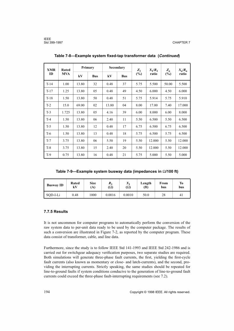
IEEEStd 399-1997 CHAPTER 7
194 Copyright © 1998 IEEE. All rights reserved.
7.7.5 Results
It is not uncommon for computer programs to automatically perform the conversion of the
raw system data to per-unit data ready to be used by the computer package. The results of
such a conversion are illustrated in Figure 7-2, as reported by the computer program. These
data consist of transformer, cable, and line data.
Furthermore, since the study is to follow IEEE Std 141-1993 and IEEE Std 242-1986 and is
carried out for switchgear adequacy verification purposes, two separate studies are required.
Both simulations will generate three-phase fault currents, the first, yielding the first-cycle
fault currents (also known as momentary or close- and latch-currents), and the second, pro-
viding the interrupting currents. Strictly speaking, the same studies should be repeated for
line-to-ground faults if system conditions conducive to the generation of line-to-ground fault
currents could exceed the three-phase fault-interrupting requirements (see 7.2).
T-14 1.00 13.80 32 0.48 37 5.75 5.500 50.00 5.500
T-17 1.25 13.80 05 0.48 49 4.50 6.000 4.50 6.000
T-18 1.50 13.80 50 0.48 51 5.75 5.914 5.75 5.910
T-2 15.0 69.00 02 13.80 04 8.00 17.00 7.40 17.000
T-3 1.725 13.80 05 4.16 39 6.00 8.000 6.00 8.000
T-4 1.50 13.80 06 2.40 11 5.50 6.500 5.50 6.500
T-5 1.50 13.80 12 0.48 17 6.75 6.500 6.75 6.500
T-6 1.50 13.80 13 0.48 18 5.75 6.500 5.75 6.500
T-7 3.75 13.80 06 5.50 19 5.50 12.000 5.50 12.000
T-8 3.75 13.80 15 2.40 20 5.50 12.000 5.50 12.000
T-9 0.75 13.80 16 0.48 21 5.75 5.000 5.50 5.000
Table 7-9—Example system busway data (impedances in
Ω/100 ft)
Busway IDRated
kVSize(A)
R1(Ω)
X1(Ω)
Length(ft)
From bus
Tobus
SQD-I-Li 0.48 1000 0.0016 0.0010 50.0 28 41
Table 7-8—Example system fixed-tap transformer data (Continued)
XMRID
RatedMVA
Primary SecondaryZ1
(%)X1/R1ratio
Zo(%)
Xo/Roratio
kV Bus kV Bus
IEEESHORT-CIRCUIT STUDIES Std 399-1997
Copyright © 1998 IEEE. All rights reserved. 195
Table 7-10—Example system cable data (impedances in Ω/1000 ft)
CableID
kVLength
(ft)Frombus
Tobus
R1(Ω)
X1(Ω)
Ro(Ω)
Xo(Ω)
C-E1 13.8 650 03 09 0.04404 0.03668 0.0808 0.07336
C-E2 13.8 1833 09 25 0.04404 0.03668 0.08808 0.07336
C-E3 13.8 75.0 09 13 0.04404 0.03668 0.08808 0.07336
C-E4 13.8 165.0 09 12 0.04404 0.03668 0.08808 0.07336
C-F1 13.8 325.0 03 05 0.04404 0.03668 0.08808 0.07336
C-G1 13.8 680.0 03 26 0.04404 0.03668 0.08808 0.07336
C-H1 13.8 471.0 03 06 0.04404 0.03668 0.08808 0.07336
C-I1 13.8 980.0 04 15 0.04404 0.03668 0.08808 0.07336
C-J2 13.8 619.0 04 27 0.04404 0.03668 0.08808 0.07336
C-J3 13.8 1187.0 16 04 0.04404 0.03668 0.08808 0.07336
C-J4 13.8 200.0 10 13 0.04404 0.03668 0.08808 0.07336
C-J5 13.8 10.0 10 12 0.04404 0.04214 0.08808 0.08429
C-J6 13.8 475.0 10 27 0.04404 0.03668 0.08808 0.07336
C-L1 13.8 510.0 04 08 0.02831 0.03424 0.05661 0.06847
C-M1 13.8 510.0 04 24 0.04404 0.03668 0.08808 0.07336
C-M2 13.8 340.0 24 31 0.04404 0.03668 0.08808 0.07336
C-M3 13.8 485.0 24 32 0.04404 0.03668 0.08808 0.07336
C-T10-1 0.48 50.0 28 38 0.02801 0.02699 0.05602 0.05399
C-T10-2 0.48 20.0 33 28 0.04393 0.02823 0.08786 0.05645
C-T11-1 0.48 66.0 29 38 0.04393 0.02699 0.05602 0.05399
C-T11-2 0.48 20.0 34 29 0.04393 0.02823 0.08786 0.05645
C-T12-1 0.48 50.0 38 30 0.02801 0.02699 0.05602 0.05399
C-T12-2 0.48 20.0 35 30 0.04393 0.02823 0.08786 0.05645
C-T5-1 0.48 20.0 22 17 0.04393 0.02823 0.08786 0.05645
C-T6-1 0.48 20.0 23 18 0.04393 0.02823 0.08786 0.05645
C1A 13.80 2000.0 50 03 0.02314 0.04622 0.02083 0.41595
IEEEStd 399-1997 CHAPTER 7
196 Copyright © 1998 IEEE. All rights reserved.
Table 7-11—Example system synchronous motor data
Motor IDMotorbus #
RatedkV
RatedkVA
Ratedhp
r/minX"d(%)
X/Rratio
M-FDR-L 8 13.8 9000 9000 1800 20.0 34.0
Table 7-12—Example system induction motor data
MotorID
Motorbus #
Totalhp
Total kVA
r/minRated
kVXM(%)
X/Rratio
Compo-sition(hp)
M-30 51 200.0 200.0 1800 0.480 16.7 7.00 >50
M-31 51 600.0 570.0 1800 0.480 16.7 12.00 <50
M-T10-1 28 400.0 400.0 1800 0.480 16.7 10.00 <50
M-T10-2 28 500.0 500.0 1800 0.480 16.7 5.00 >50
M-T10-3 33 300.0 287.5 1800 0.480 16.7 12.00 <50
M-T11-1 29 625.0 625.0 1800 0.480 16.7 10.00 >50
M-T11-2 29 465.0 465.0 1800 0.480 16.7 5.00 <50
M-T11-3 34 110.0 110.0 1800 0.480 16.7 7.00 <50
M-T12-1 30 400.0 387.9 1800 0.480 16.7 12.00 >50
M-T12-2 30 500.0 500.0 1800 0.480 16.7 5.00 <50
M-T12-3 35 300.0 287.5 1800 0.480 16.7 12.00 <50
M-T13-1 36 2500.00 2250.00 1800 2.300 16.7 32.85 >50
M-T14-1 37 700.0 678.8 1800 0.480 16.7 12.00 >50
M-T14-2 37 300.0 300.0 1800 0.480 16.7 5.00 <50
M-T17-1 49 1250.00 1250.00 1800 0.460 33.0 10.00 >1000
M-T3-1 39 1750.00 1662.50 1800 4.160 16.7 29.74 >1000
M-T4-1 11 500.0 475.0 1800 2.400 16.7 12.00 >50
M-T5-1 17 850.0 824.2 1800 0.480 16.7 10.00 <50
M-T5-2 17 500.0 500.0 1800 0.480 16.7 5.00 >50
M-T5-3 22 150.0 142.5 1800 0.480 16.7 14.00 <50
M-T6-1 18 850.0 824.2 1800 0.480 16.7 10.00 <50
M-T6-2 18 500.0 500.0 1800 0.480 16.7 5.00 >50
IEEESHORT-CIRCUIT STUDIES Std 399-1997
Copyright © 1998 IEEE. All rights reserved. 197
M-T6-3 23 150.0 142.5 1800 0.480 16.7 14.00 <50
M-T7-1 19 1250.00 1125.00 1800 2.400 16.7 26.10 >1000
M-T7-2 19 2500.00 2375.00 1800 2.400 16.7 15.00 >1000
M-T8-1 20 1750.00 1662.50 1800 2.400 16.7 15.00 >1000
M-T8-2 20 2000.00 1800.00 1800 2.400 28.0 26.00 >1000
M-T9-1 21 750.0 727.3 1800 0.480 16.7 12.00 <50
NOTE—The motor load M-T17-1 at bus 49 (RECT) signifies a dc rectifier load and has been mod-eled as an induction motor. The reactance was taken to be 33% (0.33 p.u.) considering the rated MVAof the associated converter transformer, in accordance with Internationally accepted recommenda-tions. The dc rectifier load will be considered only for first-cycle simulation purposes and ignored forinterrupting duty.
From bus #
Tobus #
Crkt #
ImpedancesFrom
kVTokV
Tap
R(p.u.) X(p.u.) R(p.u.)
1 3 1 .00313 .05324 0.0 69.00 13.800 1.00
2 4 1 .00313 .05324 0.0 69.00 13.800 1.00
5 39 1 .04314 .34514 0.0 13.80 4.160 1.00
5 49 1 .05918 .35510 0.0 13.80 .480 1.00
6 11 1 .05575 .36240 0.0 13.80 2.400 1.00
6 19 1 .01218 .14616 0.0 13.80 2.400 1.00
12 17 1 .06843 .44477 0.0 13.80 .480 1.00
13 18 1 .05829 .37888 0.0 13.80 .480 1.00
15 20 1 .01218 .14616 0.0 13.80 2.400 1.00
16 21 1 .15036 .75178 0.0 13.80 .480 1.00
25 28 1 .05829 .37888 0.0 13.80 .480 1.00
26 29 1 .05829 .37888 0.0 13.80 .480 1.00
27 30 1 .05829 .37888 0.0 13.80 .480 1.00
Figure 7-2—Positive sequence system branch data (p.u., 10 MVA)
Table 7-12—Example system induction motor data (Continued)
MotorID
Motorbus #
Totalhp
Total kVA
r/minRated
kVXM(%)
X/Rratio
Compo-sition(hp)
IEEEStd 399-1997 CHAPTER 7
198 Copyright © 1998 IEEE. All rights reserved.
31 36 1 .02289 .22886 0.0 13.80 2.400 1.00
32 37 1 .10286 .56573 0.0 13.80 .480 1.00
50 51 1 .06395 .37796 0.0 13.80 .480 1.00
3 5 1 .00075 .00063 0.0
3 6 1 .00109 .00091 0.0
3 9 1 .00150 .00125 0.0
3 26 1 .00157 .00131 0.0
4 8 1 .00076 .00092 0.0
4 15 1 .00227 .00189 0.0
4 24 1 .00118 .00098 0.0
4 16 1 .00274 .00229 0.0
4 27 1 .00143 .00119 0.0
9 12 1 .00038 .00032 0.0
9 25 1 .00424 .00353 0.0
10 13 1 .00046 .00039 0.0
10 27 1 .00110 .00091 0.0
17 22 1 .03813 .02451 0.0
18 23 1 .03813 .02451 0.0
24 31 1 .00079 .00065 0.0
24 32 1 .00112 .00093 0.0
28 33 1 .03813 .02451 0.0
28 41 1 .03429 .02105 0.0
29 34 1 .03813 .02451 0.0
29 38 1 .08024 .07732 0.0
29 38 2 .08024 .07732 0.0
30 35 1 .03813 .02451 0.0
50 3 1 .00243 .00485 0.0
50 3 2 .00243 .00485 0.0
From bus #
Tobus #
Crkt #
ImpedancesFrom
kVTokV
Tap
R(p.u.) X(p.u.) R(p.u.)
Figure 7-2—Positive sequence system branch data (p.u., 10 MVA) (Continued)
IEEESHORT-CIRCUIT STUDIES Std 399-1997
Copyright © 1998 IEEE. All rights reserved. 199
Both studies are needed for medium- and high-voltage breaker calculations (above 1kV)
while only the first one is needed for low-voltage breakers (below 1 kV). The generator
impedances utilized for the first cycle and interrupting duty studies are shown in Figure 7-3
(from Table 7-2). The motor impedances used for momentary and Interrupting calculations
are shown in Figure 7-4 (from Table 7-2). It can be seen that small induction motors (individ-
ual motors or groups of motors composed from motors smaller than 50 hp) are neglected for
interrupting duty calculations (Table 7-2).
1000 1 1 .00139 .00296 0.0
1000 2 1 .00139 .00296 0.0
Generatorbus #
Bus kV
Generator impedances
R'd X'd R"d X"d
4 13.80 0.003 0.102 0.003 0.102
50 13.80 0.002 0.072 0.002 0.072
100 69.00 0.000 0.010 0.000 0.010
Figure 7-3—Generator impedances for momentary and
interrupting duty (p.u., 10 MVA)
Motorbus #
Bus kV
MotorMotorMVA
Motor impedances
# Type Rmom Xmom Rinter Xinter
11 2.40 1 IM 0.4750 0.352 4.219 0.879 10.547
17 0.48 1 IM 0.8242 0.338 3.384
17 0.48 1 IM 0.5000 0.802 4.008 2.004 10.020
18 0.48 1 IM 0.8242 0.338 3.384
18 0.48 1 IM 0.5000 0.802 4.008 2.004 10.020
Figure 7-4—Motor impedances for momentary and
interrupting duty (p.u., 10 MVA)
From bus #
Tobus #
Crkt #
ImpedancesFrom
kVTokV
Tap
R(p.u.) X(p.u.) R(p.u.)
Figure 7-2—Positive sequence system branch data (p.u., 10 MVA) (Continued)
IEEEStd 399-1997 CHAPTER 7
200 Copyright © 1998 IEEE. All rights reserved.
Typical information pertinent to first-cycle duty calculations is shown in Table 7-4. The sym-
metrical first cycle fault currents along with the total asymmetrical rms currents using the
standard 1.6 multiplier (assuming an X/R ratio of 25 or less), as well as using the asymmetri-
19 2.40 1 IM 1.1250 0.057 1.484 0.085 2.227
19 2.40 1 IM 2.3750 0.047 0.703 0.070 1.055
20 2.40 1 IM 1.6625 0.067 1.005 0.100 1.507
20 2.40 1 IM 1.8000 0.060 1.556 0.090 2.333
21 0.48 1 IM 0.7273 0.320 3.835
22 0.48 1 IM 0.1425 1.398 19.571
23 0.48 1 IM 0.1425 1.398 19.571
28 0.48 1 IM 0.5000 0.697 6.972
28 0.48 1 IM 0.4000 0.802 4.008 2.004 10.020
29 0.48 1 IM 0.6250 0.321 3.206 0.802 8.016
29 0.48 1 IM 0.4650 1.199 5.998
30 0.48 1 IM 0.3879 0.431 5.166 1.077 12.916
30 0.48 1 IM 0.5000 1.116 5.578
33 0.48 1 IM 0.2875 0.809 9.701
34 0.48 1 IM 0.1100 3.621 25.354
35 0.48 1 IM 0.2875 0.809 9.701
36 2.40 1 IM 2.2500 0.025 0.818 0.062 2.045
37 0.48 1 IM 0.6788 0.246 2.952 0.615 7.381
37 0.48 1 IM 0.3000 1.859 9.296
39 4.16 1 IM 1.6625 0.034 1.005 0.051 1.507
49 0.48 1 IM 1.2500 0.264 2.640
51 0.48 1 IM 0.2000 1.432 10.020 3.579 25.050
51 0.48 1 IM 0.5700 0.408 4.893
8 13.80 1 SM 9.0000 0.006 0.222 0.010 0.333
Motorbus #
Bus kV
MotorMotorMVA
Motor impedances
# Type Rmom Xmom Rinter Xinter
Figure 7-4—Motor impedances for momentary and
interrupting duty (p.u., 10 MVA) (Continued)
IEEESHORT-CIRCUIT STUDIES Std 399-1997
Copyright © 1998 IEEE. All rights reserved. 201
cal multiplier, calculated from the actual system X/R ratio at the fault point. Similar informa-
tion is shown for the peak currents. First-cycle asymmetrical fault currents are used to assess
the closing and latching duty of medium- and high-voltage circuit breakers. These currents
can be either total asymmetrical rms currents (ANSI C37.06-1979) or peak currents (ANSI
Std C37.06-1987).
Typical information pertinent to interrupting duty calculations is shown in Figure 7-6. The
same type of information as in Figure 7-5 is essentially displayed, except that in this case the
multipliers applicable to both local and remote contributions are reported with reference to
both breaker rating structures covered in IEEE Std C37.010-1979 and IEEE Std C37.5-1979.
Total asymmetrical interrupting currents are also reported, thus yielding the interrupting
requirements.
Fault at bus Prefault
# ID Zone Voltage (kV) Angle (degrees)
19 T7SEC 5 2.40 0.00
Current during fault Voltage-to-ground during fault
Type p.u. Degrees Amperes MVA p.u.Angle
(degrees)Module
(kV)
LLL-A 7.67 –85.54 18 449 77 0.00 0.00 0.00
Equivalent impedance (p.u.)X/R (IEEE Std C37.010-1979)
Xeq (IEEE Std C37.010-1979)
ZQQ-1 = 0.0101 + j0.1300 13.69 0.1300
Total asymmetrical first-cycle current
Based on 1.6 multiplier (IEEE Std C37.010-1979) Based on actual X/R ratio
18 449 × 1.60 = 29 520 A 18 449 × 1.505 = 27 765 A
Peak current
Based on 2.7 multiplier Based on actual X/R ratio
18 449 × 2.70 = 49 812 A 18 449 × 2.541 = 46 879 A
First ring contributions from:
Bus Prefault
# ID Zone Voltage (kV) Angle (degrees)
6 FDR-H 2 1 13.80 0.00
Current during fault Voltage-to-ground during fault
Type p.u. Degrees Amperes MVA p.u.Angle
(degrees)Module
(kV)
LLL-A 5.57 –85.11 13 418 56 0.82 –29.87 6.51
Transfer impedance (p.u.)
ZQP-1 = 0.0021 + j0.0236
Figure 7-5—Typical results for first cycle duty calculations
IEEEStd 399-1997 CHAPTER 7
202 Copyright © 1998 IEEE. All rights reserved.
First ring contribution from:
1 ind. motor(s) each rated 1.13 MVA
Current during fault
Type p.u. Degrees Amperes MVA
LLL-A 0.67 –87.81 1619 7
First ring contribution from:
1 ind. motor(s) each rated 2.38 MVA
Current during fault
Type p.u. Degrees Amperes MVA
LLL-A 1.42 –86.19 3414 14
Fault at bus Prefault
# ID Zone Voltage (kV) Angle (degrees)
10 EMERG 2 13.80 0.00
Current during fault Voltage-to-ground during fault
Type p.u. Degrees Amperes MVA p.u.Angle
(degrees)Module
(kV)
LLL-A 27.77 –83.05 11 616 278 0.00 0.00 0.00
Equivalent impedance (p.u.)X/R (IEEE Std C37.010-1979)
Xeq (IEEE Std C37.010-1979)
ZQQ-1 = 0.0044 + j0.0358 8.950 0.0360
Local and remote contribution from generating stations
Local/total Remote/total
49.2% 50.8%
Asymmetrical multipliers for 5 cycle breakers/3 cycles parting time (IEEE Std C37.010-1979)
IEEE StdC37.010-1979 (local)
IEEE StdC37.010-1979
(remote)
IEEE StdC37.5-1979 (local)
IEEE StdC37.5-1979 (remote)
1.00 1.00 1.00 1.00
Total asymmetrical interrupting fault currents
IEEE StdC37.010-1979 (weighted)
IEEE StdC37.010-1979
(remote)
IEEE StdC37.5-1979 (weighted)
IEEE StdC37.5-1979 (weighted)
11619 A 11619 A 11619 A 11619 A
First ring contributions from:
Bus Prefault
# ID Zone Voltage (kV) Angle (degrees)
13 T6PRI 1 13.80 0.00
Figure 7-6—Typical results for interrupting duty calculations
Figure 7-5—Typical results for first cycle duty calculations (Continued)
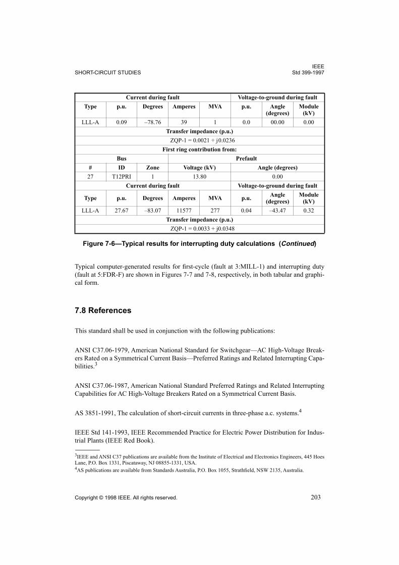
IEEESHORT-CIRCUIT STUDIES Std 399-1997
Copyright © 1998 IEEE. All rights reserved. 203
Typical computer-generated results for first-cycle (fault at 3:MILL-1) and interrupting duty
(fault at 5:FDR-F) are shown in Figures 7-7 and 7-8, respectively, in both tabular and graphi-
cal form.
7.8 References
This standard shall be used in conjunction with the following publications:
ANSI C37.06-1979, American National Standard for Switchgear—AC High-Voltage Break-
ers Rated on a Symmetrical Current Basis—Preferred Ratings and Related Interrupting Capa-
bilities.3
ANSI C37.06-1987, American National Standard Preferred Ratings and Related Interrupting
Capabilities for AC High-Voltage Breakers Rated on a Symmetrical Current Basis.
AS 3851-1991, The calculation of short-circuit currents in three-phase a.c. systems.4
IEEE Std 141-1993, IEEE Recommended Practice for Electric Power Distribution for Indus-
trial Plants (IEEE Red Book).
Current during fault Voltage-to-ground during fault
Type p.u. Degrees Amperes MVA p.u. Angle (degrees)
Module(kV)
LLL-A 0.09 –78.76 39 1 0.0 00.00 0.00
Transfer impedance (p.u.)
ZQP-1 = 0.0021 + j0.0236
First ring contribution from:
Bus Prefault
# ID Zone Voltage (kV) Angle (degrees)
27 T12PRI 1 13.80 0.00
Current during fault Voltage-to-ground during fault
Type p.u. Degrees Amperes MVA p.u.Angle
(degrees)Module
(kV)
LLL-A 27.67 –83.07 11577 277 0.04 –43.47 0.32
Transfer impedance (p.u.)
ZQP-1 = 0.0033 + j0.0348
3IEEE and ANSI C37 publications are available from the Institute of Electrical and Electronics Engineers, 445 HoesLane, P.O. Box 1331, Piscataway, NJ 08855-1331, USA.4AS publications are available from Standards Australia, P.O. Box 1055, Strathfield, NSW 2135, Australia.
Figure 7-6—Typical results for interrupting duty calculations (Continued)
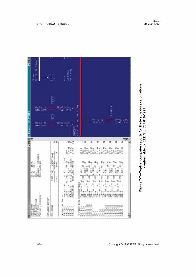
IEEESHORT-CIRCUIT STUDIES Std 399-1997
204 Copyright © 1998 IEEE. All rights reserved.
Fig
ure
7-7
—Typ
ical
co
mp
ute
r re
po
rts f
or
firs
t-cycle
du
ty c
alc
ula
tio
ns
co
nfo
rmab
le t
o I
EE
E S
td C
37.0
10-1
979
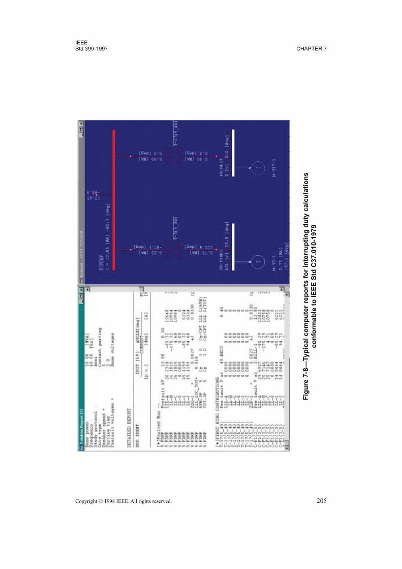
IEEEStd 399-1997 CHAPTER 7
Copyright © 1998 IEEE. All rights reserved. 205
Fig
ure
7-8
—Typ
ical
co
mp
ute
r re
po
rts f
or
inte
rru
pti
ng
du
ty c
alc
ula
tio
ns
co
nfo
rmab
le t
o I
EE
E S
td C
37.0
10-1
979
IEEEStd 399-1997 CHAPTER 7
206 Copyright © 1998 IEEE. All rights reserved.
IEEE Std 241-1990 (Reaff 1997), IEEE Recommended Practice for Electric Power Systems
in Commercial Buildings (IEEE Gray Book).
IEEE Std 242-1986 (Reaff 1991), IEEE Recommended Practice for Protection and Coordina-
tion of Industrial and Commercial Power Systems (IEEE Buff Book).
IEEE Std C37.010-1979, IEEE Application Guide for AC High-Voltage Circuit Breakers
Rated on a Symmetrical Current Basis (includes supplement Std C37.010d).
IEEE Std C37.5-1979, IEEE Guide for Calculation of Fault Currents for Application of AC
High-Voltage Circuit Breakers Rated on a Total Current Basis.5
IEEE Std C37.13-1990, IEEE Standard for Low-Voltage AC Power Circuit Breakers Used in
Enclosures.
VDE 0102, Recommendation for the Calculation of Short Circuit Currents, Part 1: Three
Phase systems of voltages above 1 KV, Issued by the Deutsche Elektrotechnische Kommis-
sion, Frankfurt, Germany, 1972 (VDE).
IEC 60909 (1988), Short-circuit current calculation in three phase a.c. systems.6
7.9 Bibliography
[B1] Anderson, P., Analysis of Faulted Power Systems, IEEE Power System Engineering
Series, Piscataway, NJ: IEEE Press, 1995.
[B2] Arrilaga J., Arnold, C. P, and Harker, B. J., Computer Modelling of Electrical Power
System, New York: John Wiley & Sons, 1983.
[B3] Blackburn, L. J., Symmetrical Components for Power Systems Engineering, New York:
Marcel Dekker, Inc., 1993.
[B4] Huening, W. C., Calculating short-circuit currents with contributions from induction
motors, IEEE Transactions on Industry Applications, vol. IA-18, pp. 85–92, Mar./Apr. 1982.
[B5] Huening, W. C., Interpretation of new American National Standards for power circuit
breaker applications. IEEE Transactions on Industry and General Applications, vol. IGA-5,
Sep./Oct. 1969.
[B6] NFPA 70-1966, National Electric Code® (NEC®).
5This Standard has been withdrawn. Copies can be obtained for the IEEE Standards Department at (908) 562-3821.6IEC publications are available from IEC Sales Department, Case Postale 131, 3, rue de Varembé, CH-1211, Genève20, Switzerland/Suisse. IEC publications are also available in the United States from the Sales Department, Ameri-can National Standards Institute, 11 West 42nd Street, 13th Floor, New York, NY 10036, USA.
IEEESHORT-CIRCUIT STUDIES Std 399-1997
Copyright © 1998 IEEE. All rights reserved. 207
[B7] Rodolakis, A. J., A comparison of North American (ANSI) and European (IEC) Fault
calculation guidelines, IEEE Transactions on Industry Applications, vol. 29, No. 3, pp. 515–
521, May/June 1993.
[B8] Roeper, R., Short Circuit Currents in Three Phase Systems, Siemens Actiengesellschaft,
John Wiley & Sons, 1985.
[B9] Stagg, G. W., and El-Abiad, A. H., Computer Methods in Power System Analysis, New
York: McGraw-Hill, 1968.
[B10] Stevenson, W. D., Elements of Power System Analysis, New York: McGraw-Hill, 1982.
[B11] St. Pierre, C. R., Time Sharing Computer Programs (DATUMS) for Power Data Reduc-
tion. Schenectady, NY: General Electric Company, 1973.
[B12] Tinney W., Brandwajn, V., and Chan, S., Sparse Vector Methods, IEEE Transactions on
Power Apparatus and Systems, vol. PAS 104, pp. 295–301, Feb. 1985.
[B13] Wagner, C. F., and Evans, R. D., Symmetrical Components, New York: McGraw-Hill,
1933.