Embed Size (px)
Citation preview
136
Chapter 5
Face Recognition Using Vector Quantization
(VQ) Techniques
5.1 Introduction
Automatic facial recognition is an attractive solution for the problem
of automatic personal identification systems. In order to facilitate a
cost effective solution high levels of data reduction are required
when storing the facial information. Image compression is a fast
paced and dynamically changing field with many different varieties
of compression methods available.
Image compression using Vector Quantization (VQ) [97-105] has
received great attention in the last decades because it‘s promising
compression ratio and relatively simple structure. This analyzes the
image as a two dimensional signal and takes advantage of
redundancies associated with the human visual system (HVS).
Vector Quantization (VQ) can be used as data reduction technique
for the encoding of facial images.
5.2 Definition of Vector Quantization
A vector quantizer Q of dimension k and size N is a mapping from a
point in k-dimensional Euclidean space, Rk into a finite set C
containing N output or reproduction points that exist in the same
Euclidean space as the original point. These reproduction points are
known as code-words and these set of code-words are called a
codebook C with N distinct code- vectors in the set. Thus the
mapping function Q is defined as,
Q : Rk C
5.1
137
The number of codevectors (N) depends on two parameters
Rate (R) (bits/pixel)
Dimension (L)(grouping)
The number of code vectors required is calculated using following
equation
Number of code vector (N)= 2R.L 5.2
When the rate increases the codebook size as well as complexity
also increases.
Vector quantization in its entirety is quite a simple concept. The
major complexity comes about in selecting a codebook C of size N
that best represents original vectors or training set X in Rk
Euclidean space.
The representative codeword is determined to be the closest in
Euclidean distance from the input vector. The Euclidean distance is
defined by
k
j
ijji yxyxd1
2)(),(
5.3
where xj is the jth component of the input vector and yij is the jth is
component of the codeword yi. [117]
5.3 Advantages of Vector Quantization
A vector can be used to describe almost all types of patterns that
arise in digital images. Vector Quantization can be viewed as a form
of pattern recognition where an input pattern is approximated by a

138
vector contained in a stored set of code-words. If this codebook has
less patterns in it than in the original training set then compression
can be achieved. For all these reasons several vector quantization
schemes have been developed to take advantage of the inherent
redundancies in digital images. Vector Quantization is commonly
used to compress data that have been digitized from an analog
source such as sampled sound and scanned images. VQ is based on
two facts:
1. Compression method that compresses strings rather
than individual symbols can in principle produces better
results.
2. Adjacent data blocks in an image are correlated.
Based on the above characteristics VQ has following advantages
1. Using VQ very high compression ratio can be obtained.
So saving of storage space can be achieved.
2. Multimedia applications make extensive use of images
and video. Such multimedia applications will only be
feasible with compression methods. The storage space
saved due to compression allows a greater number of
images to be stored.
3. High Transmission rates are possible because in VQ
method only index is transmitted for a particular block
and receiver can reconstruct the massage using this
index.
4. Compression increases transmission rate that in turn
improves the utility of bandwidth and time saving.

139
5. In VQ image decompression is very quick since it
consists mainly of look up table operation. In a typical
type of image database application an image is
compressed once when it is first archived into the
system. It is subsequently decompressed many times.
Vector quantization algorithms for reducing bit storage have been
extensively investigated over recent years. To accomplish the VQ
techniques a vector quantizer is designed which is a system for
mapping a sequence of continuous or discrete vectors into a digital
sequence suitable for storage. The main reason for doing this is to
reduce the rate for transmission of an image while maintaining an
acceptable image quality. The reason this method of compression
has gained such interest over conventional means for compression
(i.e. Digital Pulse Code Modulation (DPCM), Transform coding etc.)
is that these conventional methods usually employ scalar
quantization in some manner. Scalar quantization is not optimal as
successive samples in a digital signal are usually correlated or
dependent.
VQ exploits the correlation existing between neighbouring signal
samples by quantizing them together. In general VQ scheme can be
divided into two parts:
The encoding procedure
The decoding procedure
A simple block diagram of vector quantizer is shown in following Fig
5.1

140
The Encoder The Decoder
Fig. 5.1 Block diagram of Vector Quantizer
At the encoder the input image is partitioned into a set of non
overlapping image blocks. The closest code word in the codebook is
then found for each image block using Euclidean distance as a
similarity measure. The corresponding index for each searched
closest code words in the code book are sent to the decoder as
shown in Fig.5.1.
A number of different vector quantization (VQ) schemes exists that
take advantage of different characteristics of a digital signal
depending on the type of pattern matching technique required. This
is very useful as images contain areas that are more perceptually
important than other regions of that same image. Using these
varied vector quantization techniques it is possible to take
advantage of some of the psychovisual redundancies that exist in
digitally stored images. The goal of VQ code book generation is to
find an optimal code book that yields the lowest possible distortion
when compared with all other code books of same size. The VQ
performance is directly proportional to code book size and the
vector size. The minimization of this distortion is the key that makes
Search
Engine
Output Vector Input Vector
Code-book Indices Indices Code-book
Channel

141
vector quantization work so well and as with all other compression
schemes. This minimization is closely related to the statistics of the
vectors to be quantized.
5.4 Algorithm Development
The performance of VQ relies on having a good set of vectors in its
codebook. For image compression these vectors are chosen to
minimize the overall pixel level error introduced. However for face
recognition other considerations are also important. For example
individuality may be more significant than pixel error when encoding
facial features. There are many different algorithms available which
perform codebook generation.
In this particular thesis following algorithms are studied and its
performance is compared in terms of percentage accuracy for face
recognition under normal conditions, Occlusion and also in presence
of different noise.
Codebook Design Algorithms
1. LBG Algorithm
2. K-Means Algorithm
3. Kekre‘s Fast codebook Generation Algorithm (KFCG)
5.4.1 LBG Algorithm
The Linde, Buzo, Gray (LBG) algorithm [106] is used to design the
codebook. The algorithm iteratively minimizes the total distortion by
representing the training vectors by their corresponding code
vectors. The LBG algorithm is an iterative algorithm in which the

142
codebook C is obtained by splitting method. In this algorithm
centroid is computed as the first codevector C1 for the training set.
In Fig.5.2 two vectors v1 & v2 are generated by adding constant
error to the centroid C1. Euclidean distances of all the training
vectors are computed with vectors v1 & v2 and two clusters are
formed based on nearest of v1 or v2. This procedure is repeated for
every new cluster until the required size of codebook is reached or
specified Mean Square Error (MSE) is reached.
Fig 5.2 Graphical representation of cluster generation for LBG
algorithm
5.4.1.1 Face Recognition using LBG Algorithm
The LBG algorithm is a clustering algorithm. This algorithm is
applied first on the whole database for preparation of a code book
of various sizes

143
Fig.5.3 Code book preparation using LBG algorithm for the
facial databases.
As shown in the Fig. 5.3 the database images are divided into the
block of 2x2 pixels from each block are arranged in a single row.
Then the mean of the each column is calculated. This mean value is
a coordinate for the first codevector C1. After that a constant error
of +1 and -1 is added to the C1 to get two more code vectors. The
existing blocks are now compared with the newly generated code
vectors C1‘ and C1‘‘ respectively and for each of them the
Euclidiean distance is calculated. Whichever code vector gives
minimum Euclidiean distance the blocks are place in that particular
cluster. So after first iteration two different and non overlapping
clusters are formed. For these clusters now the procedure is
repeated to get clusters in multiple of two and code book is
prepared.
In this particular chapter the code book size of 32, 64, 128 and 256
are generated using LBG algorithm.
Following are the steps for LBG technique for face recognition
(image size is 64x64)
The test image is divided into blocks of 2*2
The pixels are then arranged into an array of 1024*4 vectors.

144
Then the mean of these vectors is calculated.
Mean+1 and mean-1 is taken as code vectors Euclidean
distance of each training vector from training set of 1024 *4
vectors is compared to form two clusters.
Mean of these new clusters is calculated individually. Add
mean+1 and mean-1 to form 4 clusters. The process is
repeated till we get desired number of clusters (32, 64, 128,
256).
This forms the final codebook. Then the codebook of the test
image is compared with the codebook of the images in the
database and depending on the pre decided threshold value
the image is accepted or rejected.
Disadvantages of LBG algorithm are:
Since fixed error is added (Є=+1), the MSE is higher. The
generated codevectors have slope of 45o
If a particular point is equidistant from two clusters then
which cluster should include the point is not mentioned in the
algorithm.
Cluster elongation is +135o to horizontal axis in two
dimensional cases. This results in inefficient clustering.
5.4.1.2 LBG Result Analysis
The LBG clustering algorithm is tested on locally generated
unconstrained Local database and standard ORL database of At&T
lab [118]. In Indian database there were 100 persons from that 7
poses per person is taken in training set and codebook is generated
for different sizes and stored separately. The testing is done on
another 3 poses of the same person. Just for comparison two poses
at random from training set is also checked which makes total
145
(3+2=5*100) 500 testing images in all. The ORL database has 40
individuals with 10 poses each. Out of these 7 poses are selected as
training set to generate the codebook and remaining 3 poses are
selected to create a testing set.
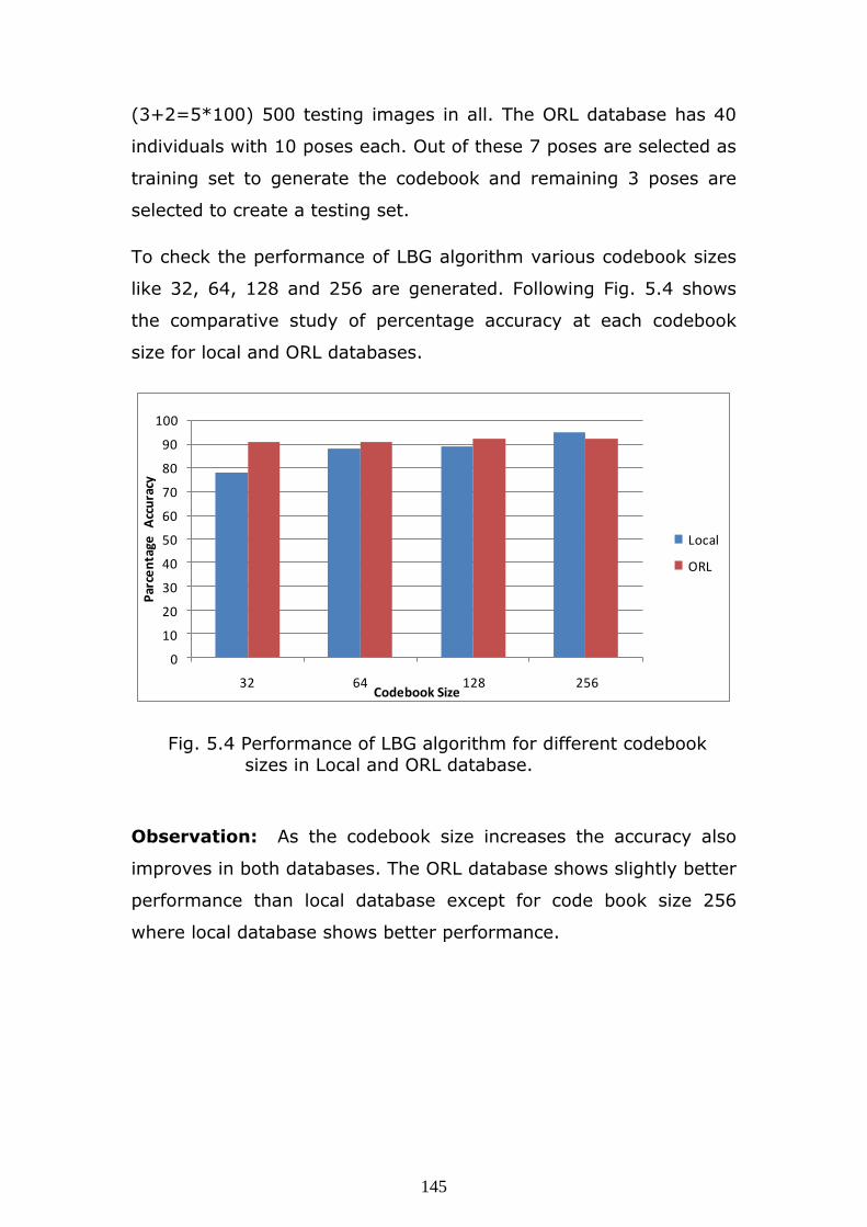
To check the performance of LBG algorithm various codebook sizes
like 32, 64, 128 and 256 are generated. Following Fig. 5.4 shows
the comparative study of percentage accuracy at each codebook
size for local and ORL databases.
0
10
20
30
40
50
60
70
80
90
100
32 64 128 256
Par
cen
tage
A
ccu
racy
Codebook Size
Local
ORL
Fig. 5.4 Performance of LBG algorithm for different codebook
sizes in Local and ORL database.
Observation: As the codebook size increases the accuracy also
improves in both databases. The ORL database shows slightly better
performance than local database except for code book size 256
where local database shows better performance.
146
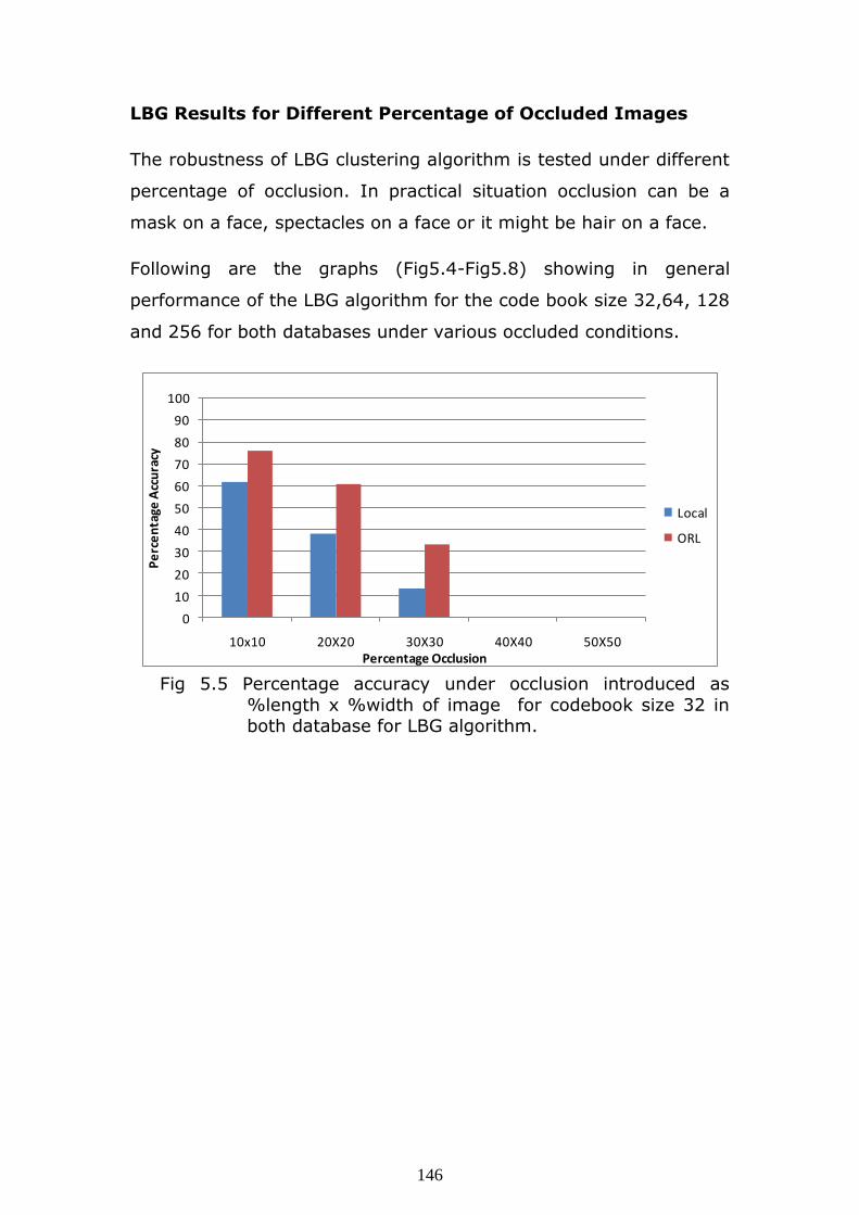
LBG Results for Different Percentage of Occluded Images
The robustness of LBG clustering algorithm is tested under different
percentage of occlusion. In practical situation occlusion can be a
mask on a face, spectacles on a face or it might be hair on a face.
Following are the graphs (Fig5.4-Fig5.8) showing in general
performance of the LBG algorithm for the code book size 32,64, 128
and 256 for both databases under various occluded conditions.
Fig 5.5 Percentage accuracy under occlusion introduced as
%length x %width of image for codebook size 32 in both database for LBG algorithm.
0
10
20
30
40
50
60
70
80
90
100
10x10 20X20 30X30 40X40 50X50
Pe
rce
nta
ge A
ccu
racy
Percentage Occlusion
Local
ORL

147
Fig5.6 Percentage accuracy under occlusion introduced as
%length x %width of image for codebook size 32 in both database for LBG algorithm.
Fig 5.7 Percentage accuracy under occlusion conditions introduced as %length X %width in image for codebook size 128
in both database for LBG algorithm.
0
10
20
30
40
50
60
70
80
90
100
10X10 20X20 30x30 40X40 50X50
Pe
rce
nta
ge A
ccu
racy
Percentage Occlusion
Local
ORL
0
10
20
30
40
50
60
70
80
90
100
10X10 20X20 30X30 40X40 50x50
Pe
rce
nta
ge A
ccu
racy
Percentage Occlusion
Local
ORL

148
Fig 5.8 Percentage accuracy under occlusion introduced as %length X %width in image for codebook size 256 in
both database for LBG algorithm.
Observations: The graphs show that as occlusion increase on
image the recognition accuracy reduces drastically. The ORL
database gives better accuracy in all codebook sizes. The code book
size 256 can withstand the occlusion upto 20%X20% only.
LBG Results for various types of Noise
The LBG algorithm for face recognition is tested for the various
types of noise introduced to the image like Speckle Noise, Salt and
pepper noise and Gaussian noise. Following are the graphs showing
in general performance of the LBG algorithm for the various
codebook sizes.
0
10
20
30
40
50
60
70
80
90
100
10X10 20X20 30X30 40X40 50X50
Pe
rce
nta
ge A
ccu
racy
Percentage Occlusion
Local
ORL

149
Speckle Noise:
0
10
20
30
40
50
60
70
80
90
100
10 20 30 40 50
Pe
rce
nta
ge A
ccu
racy
Percentage Speckle Noise
Local
ORL
Fig 5.9 Performance of LBG algorithm for Speckle Noise for codebook size 32 for both databases.
Observation: As shown in graph Fig 5.9 the LBG withstand 10%
Speckle Noise for local and ORL database for codebook size of 32.
Higher codebook sizes do not support the noise addition.

150
Gaussian Noise:
Fig5.10 Performance of LBG
algorithm for
Gaussian noise for
codebook size 32 in
both databases.
Fig 5.11 Performance of
LBG algorithm for
Gaussian noise for
codebook size 128 in
both databases.
Fig 5.12 Performance of LBG algorithm for Gaussian noise for codebook
size 256 in both databases
Observation: As shown in graphs (Fig 5.10-Fig 5.12) the LBG
withstand 1% Gaussian noise addition for local and ORL database
for codebook size of 32. Codebook size 64 does not support noise
addition at all. Codebook size 128 withstands the 1% Gaussian
noise in local database where as codebook size 256withstand 1%
Gaussian noise in ORL database.
0
10
20
30
40
50
60
70
80
90
100
1 5 10
Pe
rce
nta
ge A
ccu
racy
Percentage Gaussian Noise
Local
ORL
0
10
20
30
40
50
60
70
80
90
100
1 5 10
Pe
rcn
tage
Acc
ura
cy
Percentage Gaussian Noise
Local
ORL
0
10
20
30
40
50
60
70
80
90
100
1 5 10
Pe
rce
nta
ge A
ccu
racy
Percentage Gaussian Noise
Local
ORL

151
Salt and Pepper Noise:
Fig 5.13 Performance of LBG
algorithm for Salt and
Pepper noise for
codebook size 32 in
both databases
Fig 5.14 Performance of LBG
algorithm for Salt
and Pepper noise for
codebook size 128
for both databases.
Fig 5.15 Performance of LBG
algorithm for Salt and
Pepper noise for codebook
size 256 in both databases
0
10
20
30
40
50
60
70
80
90
100
10 20 30 40 50
Pe
rce
nta
ge A
ccu
racy
Percentage Salt and Pepper Noise
Local
ORL
0
10
20
30
40
50
60
70
80
90
100
10 20 30 40 50
Pe
rce
nta
ge A
ccu
racy
Salt and Pepper Noise
Local
ORL
0
10
20
30
40
50
60
70
80
90
100
10 20 30 40 50
Pe
rce
nta
ge A
ccu
racy
Percentage Salt and Pepper Noise
Local
ORL
152
Observation: The Salt and pepper noise addition is not tolerated
by 64 codebook size at all in both the databases. The codebook size
32 (Fig 5.13)withstands the noise addition less than 20% for both
the databases, 128 codebook size(Fig 5.14) shows good result for
local database and 256(Fig 5.15) shows the better result for ORL
database.
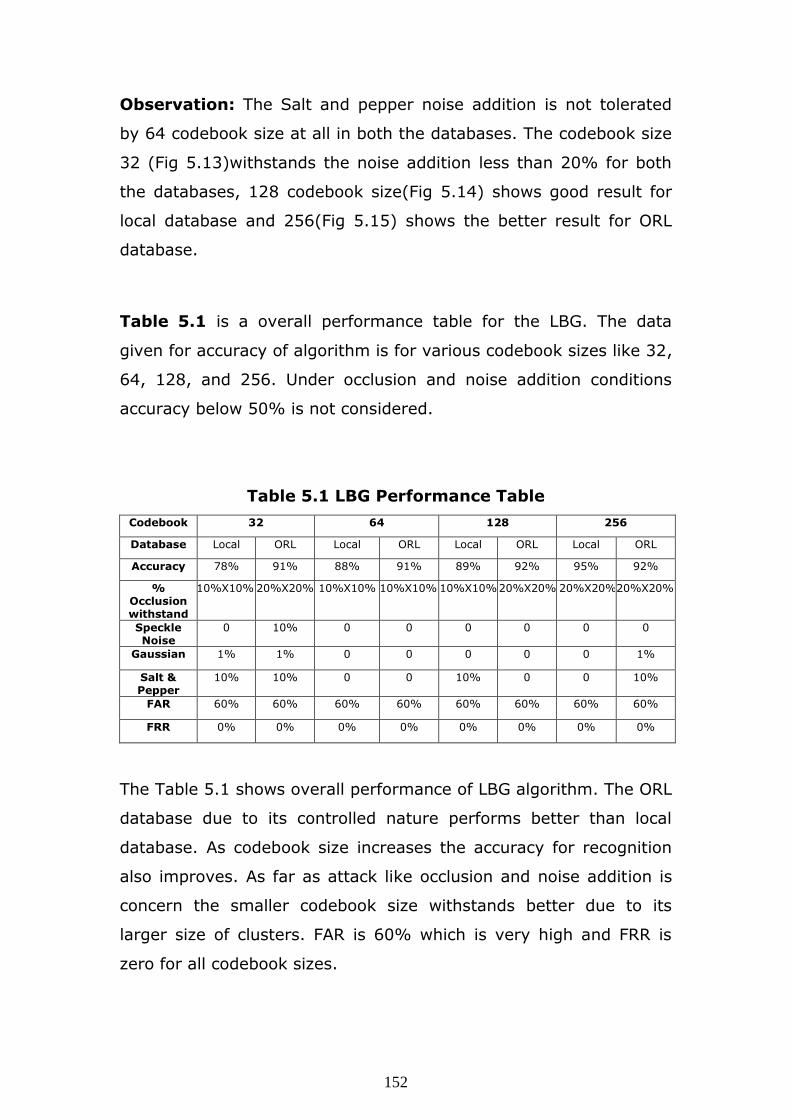
Table 5.1 is a overall performance table for the LBG. The data
given for accuracy of algorithm is for various codebook sizes like 32,
64, 128, and 256. Under occlusion and noise addition conditions
accuracy below 50% is not considered.
Table 5.1 LBG Performance Table
Codebook 32 64 128 256
Database Local ORL Local ORL Local ORL Local ORL
Accuracy 78% 91% 88% 91% 89% 92% 95% 92%
% Occlusion withstand
10%X10% 20%X20% 10%X10% 10%X10% 10%X10% 20%X20% 20%X20% 20%X20%
Speckle Noise
0 10% 0 0 0 0 0 0
Gaussian 1% 1% 0 0 0 0 0 1%
Salt & Pepper
10% 10% 0 0 10% 0 0 10%
FAR 60% 60% 60% 60% 60% 60% 60% 60%
FRR 0% 0% 0% 0% 0% 0% 0% 0%
The Table 5.1 shows overall performance of LBG algorithm. The ORL
database due to its controlled nature performs better than local
database. As codebook size increases the accuracy for recognition
also improves. As far as attack like occlusion and noise addition is
concern the smaller codebook size withstands better due to its
larger size of clusters. FAR is 60% which is very high and FRR is
zero for all codebook sizes.

153
5.4.2 K-Means Algorithm
The K-Means algorithm takes the input parameter k, and partitions
a set of n objects into k clusters so that the resulting intra cluster
similarity is high but the inter cluster similarity is low. [107]
Similarity criterion for cluster is decided based on the mean value of
object in a cluster.
K-means algorithm randomly selects k of the objects. This is taken
as initial codebook. Each of the remaining objects is assigned to the
cluster based on the distance between the object and a code vector.
It then calculates a new mean for each cluster and the process
iterates until the minimum error stabilizatizes. The K-means
procedure is summarized in following diagram (Fig 5.16).
(a) (b) (c)
Fig 5.16 Cluster formation based on the K-means method.
(The red point in diagram is a mean of each cluster.)
Disadvantages of K-Means algorithm are :
K-Means finds a local optimum and may actually miss the
global optimum.
K-Means does not work on categorical data because the mean
must be defined on the attribute type.
Only convex shaped clusters are found.

154
The K-Means algorithm is not time efficient and does not scale
well.
5.4.2.1 K-Means Algorithm Applied to Face Recognition
The initial codebook of size 32, 64,128 and 256 is prepared for
both local and ORL database. The test image or a query image is a
facial image either from testing database or outside the database.
Following are the steps for K-Means clustering algorithm for face
recognition (image size is 64x64)
Initially the test image is divided into blocks of 2*2.
Then the pixels are arranged into an array of 1024*4.
Out of these 1024 vectors, 256 random vectors are chosen
and this forms the initial codebook.
Now the 1024 vectors are compared with the initial codebook
on the basis of the Euclidean distance between the two
vectors. And then depending on the minimum Euclidean
distance, the 1024 vectors are divided into 256 clusters.
Now the average of each of these clusters is taken to form
the revised codebook.
Then the codebook of the test image is compared with the
codebook of the images in the database and depending on the
pre decided threshold value the image is accepted or rejected.
5.4.2.2 K-means Results Analysis
To check the performance of K-Means algorithm various codebook
sizes are tried like 32, 64, 128 and 256. Following Fig. 5.17 shows
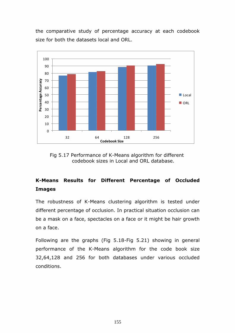
155
the comparative study of percentage accuracy at each codebook
size for both the datasets local and ORL.
0
10
20
30
40
50
60
70
80
90
100
32 64 128 256
Pe
rce
nta
ge A
ccu
racy
Codebook Size
Local
ORL
Fig 5.17 Performance of K-Means algorithm for different
codebook sizes in Local and ORL database.
K-Means Results for Different Percentage of Occluded
Images
The robustness of K-Means clustering algorithm is tested under
different percentage of occlusion. In practical situation occlusion can
be a mask on a face, spectacles on a face or it might be hair growth
on a face.
Following are the graphs (Fig 5.18-Fig 5.21) showing in general
performance of the K-Means algorithm for the code book size
32,64,128 and 256 for both databases under various occluded
conditions.

156
Fig 5.18 Percentage accuracy under occlusion introduced as
%length x %width of image for codebook size 32
in both databases.
Fig 5.19 Percentage accuracy under occlusion introduced as
%length x %width of image for codebook size 64 in
both databases.
0
10
20
30
40
50
60
70
80
90
100
10x10 20X20 30X30 40X40 50X50
Pe
rce
nta
ge A
ccu
racy
Percentage Occlusion
Local
ORL
0
10
20
30
40
50
60
70
80
90
100
10X10 20X20 30X30 40X40 50X50
Pe
rce
nta
ge A
ccu
racy
Percentage Occlusion
Local
ORL

157
Fig5.20 Percentage accuracy under occlusion introduced as
%length x %width of image for codebook size 128
in both databases.
Fig 5.21 Percentage accuracy under occlusion introduced as
%length x %width of image for codebook size 256
in both databases.
Observation: K-Means algorithm can withstand occlusion
introduced in length and width as 50%X50% for both databases. It
0
10
20
30
40
50
60
70
80
90
100
10X10 20X20 30x30 40x40 50X50
Pe
rce
nta
ge a
ccu
racy
Percentage occlusion
Local
ORL
0
10
20
30
40
50
60
70
80
90
100
10 20 30 40 50
Pe
rce
nta
ge A
ccu
racy
Percentage Occlusion
Local
ORL

158
is showing better performance compared to LBG algorithm under
occlusion.
K-Means Results for various types of Noise:
The K-Means algorithm for face recognition is tested for the various
types of noise introduced to the image like Speckle Noise, Salt and
pepper noise and Gaussian noise. Following are the graphs showing
in general performance of the K-Means algorithm for the various
codebook sizes under noise addition condition.
Speckle Noise:
Fig 5.22 Performance of K-means algorithm for Speckle noise
for various codebook sizes in local database
Observation: As shown in graph (Fig 5.22) the K-Means withstand
10% Speckle Noise addition for local database for codebook size 32
and 256 but the accuracy is not acceptable. Other codebook sizes
0
10
20
30
40
50
60
70
80
90
100
10 20 30 40 50
32
64
128
256

159
does not support the noise addition.ORL database cannot withstand
the Speckle Noise addition at all and fails to recognize the correct
face.
Gaussian Noise:
Fig 5.23 Performance of K-means algorithm for Gaussian
noise for various codebook sizes in ORL database.
Observation: As shown in graph (Fig 5.23) the K-Means withstand
1% Gaussian noise addition for ORL database for codebook size of
32. The local database is very sensitive to this noise and fails to
recognize the face correctly. Higher order codebooks also do not
support the noise addition.
0
10
20
30
40
50
60
70
80
90
100
1 5 10
Pe
rce
nta
ge A
ccu
racy
Percentage Gaussian Noise
32
64
128
256

160
0
10
20
30
40
50
60
70
80
90
100
10 20 30 40 50
Pe
rce
nta
ge A
ccu
racy
Percentage Salt & Pepper Noise
Local
ORL
Salt and Pepper Noise:
Fig 5.24 Performance of K-
means algorithm for Salt and Pepper noise
for codebook size 32 in both the databases.
Fig 5.25 Performance of K-
means algorithm for Salt
and Pepper noise for
codebook size 64 in both
the databases.
Fig 5.26 Performance of K-
means algorithm for
Salt and Pepper noise
for codebook size 128
in both the databases.
Fig 5.27 Performance of K-
means algorithm for Salt
and Pepper noise for
codebook size 256 in
both the databases.
0
10
20
30
40
50
60
70
80
90
100
10 20 30 40 50
Pe
rce
nta
ge A
ccu
racy
Percentage Salt & Pepper Noise
Local
ORL
0
10
20
30
40
50
60
70
80
90
100
10 20 30 40 50
Pe
rce
nta
ge A
ccu
racy
Percentage Salt & pepper noise
Local
ORL
0102030405060708090
100
10 20 30 40 50
Pe
rce
nta
ge A
ccu
racy
Percentage Salt & pepper noise
Local
ORL

161
Observation: Graphs (Fig 5.24-Fig 5.27) show performance of K-
means algorithm for Salt and Pepper noise analysis. The codebook
size 256 is very sensitive for addition of Salt & Pepper noise. For
10% noise addition the accuracy is only 1%.
Table 5.2 is a overall performance table for the K-Means algorithm.
The data given for accuracy of algorithm is for various codebook
sizes like 32, 64, 128, and 256. Under occlusion and noise addition
conditions the cutoff point is 50% accuracy below which algorithm is
not considered.
Table 5.2 K-Means Performance Table
Codebook 32 64 128 256
Database Local ORL Local ORL Local ORL Local ORL
Accuracy 77% 79% 82% 83% 89% 91% 92% 93%
%
Occlusion
withstand
40%X40% 40%X40% 40%X40% 40%X40% 50%X50% 50%X50% 50%X50% 50%X50%
Speckle
Noise
10% 0% 0% 0% 0% 0% 1% 0%
Gaussian 0% 1% 0% 0% 0% 0% 0% 0%
Salt &
Pepper
30% 20% 10% 0% 20% 10% 0% 0%
FAR 0% 0% 0% 0% 0% 0% 0% 0%
FRR 8% 9% 12% 12% 20% 20% 30% 30%
The Table 5.2 shows overall performance of K-Means Algorithm. The
ORL database performs better than local database for all codebook
sizes.
K-Means algorithm is sensitive to noise addition and performs
poorly in noisy conditions. It can withstand reasonable amount of
occlusion with different codebook sizes. As codebook size increase
robustness towards occlusion also increases. FAR is zero for all
codebook sizes and FRR increases with codebook size.

162
5.4.3 Kekre’s Fast Codebook Generation Algorithm
(KFCG)
The Kekre‘s Fast Codebook Generation (KFCG) algorithm [116] is a
newly suggested clustering algorithm. As its name suggest it is the
fast codebook generation method compared to existing algorithms
like LBG and K-Means.
Initially only one cluster is present with entire training vectors and
the codevector C1 which is centroid.
In the first iteration of the algorithm, the clusters are formed by
comparing first element of training vector with first element of code
vector C1. The vector Xi is grouped into the cluster-1 if xi1< c11
otherwise vector Xi is grouped into cluster-2 as shown in Fig.5.28
where codevector dimension space is 2.
In second iteration, the cluster 1 is split into two by comparing
second element xi2 of vector Xi belonging to cluster 1 with that of
the second element of the codevector. Cluster 2 is split into two by
comparing the second element xi2 of vector Xi belonging to cluster 2
with that of the second element of the codevector as shown in Fig.
5.29.
This procedure is repeated till the codebook size is reached to the
size specified by user.

163
Fig 5.28 KFCG algorithm for 2 dimensional case after first iteration.
Fig 5.29 KFCG algorithm for 2 dimensional case after second
iteration.
It is observed that this algorithm gives less error as compared to
LBG and requires least time to generate codebook as compared to

164
other algorithms as it does not require any computation of
Euclidean distance.
The general diagram for KFCG codebook generation for multiple
iteration is shown in Fig.5.29.
Following Fig 5.30 is a pictorial representation of KFCG algorithm for
multiple iterations.
Fig 5.30 KFCG algorithm for 2 dimensional case after
multiple iterations.

165
5.4.3.1 KFCG Algorithm Applied for Face Recognition
The initial codebook of size 32, 64,128 and 256 is prepared for
both local and ORL database. The test image or a query image is a
facial image either from database or outside the database.
Explanation
Initially we have all the vectors forming one cluster
In the first iteration of the algorithm, the cluster is divided by
comparing first member of training vector with mean of first
column denoted by c11.
The vector Xi is grouped into the cluster 1 if Xi (1) < c11
otherwise vector Xi is grouped into cluster2.
In second iteration, the cluster 1 is split into two by
comparing second member Xi(2) of vector Xi belonging to
cluster 1 with that of the member c12 of the codevector C1.
Cluster 2 is split into two by comparing the member xi2 of
vector Xi belonging to cluster 2 with that of the member c22
of the codevector C2.
This procedure is repeated till the codebook size is increased
to the size specified by user.
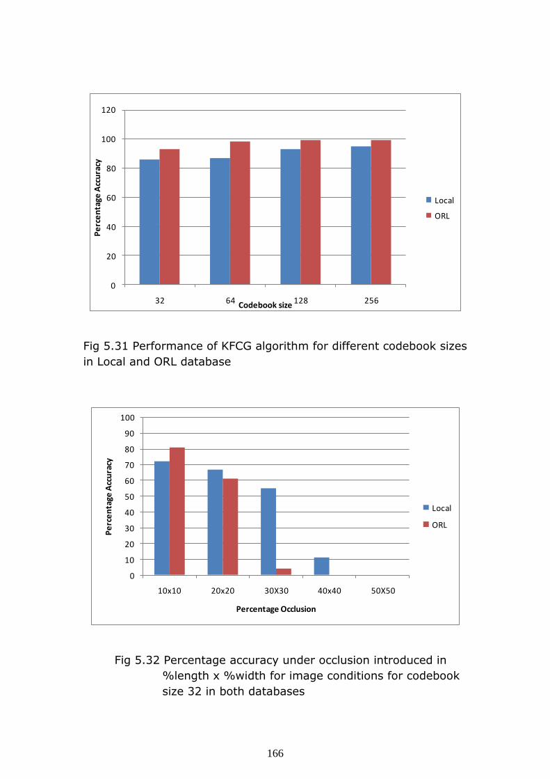
5.4.3.2 KFCG Result Analysis
To check the performance of KFCG algorithm various codebook sizes
are tried like 32, 64, 128 and 256. Following Fig. 5.31 shows the
comparative study of percentage accuracy at each codebook size for
both the datasets, local and ORL.
166
Fig 5.31 Performance of KFCG algorithm for different codebook sizes
in Local and ORL database
Fig 5.32 Percentage accuracy under occlusion introduced in
%length x %width for image conditions for codebook
size 32 in both databases
0
20
40
60
80
100
120
32 64 128 256
Pe
rce
nta
ge A
ccu
racy
Codebook size
Local
ORL
0
10
20
30
40
50
60
70
80
90
100
10x10 20x20 30X30 40x40 50X50
Pe
rce
nta
ge A
ccu
racy
Percentage Occlusion
Local
ORL
167
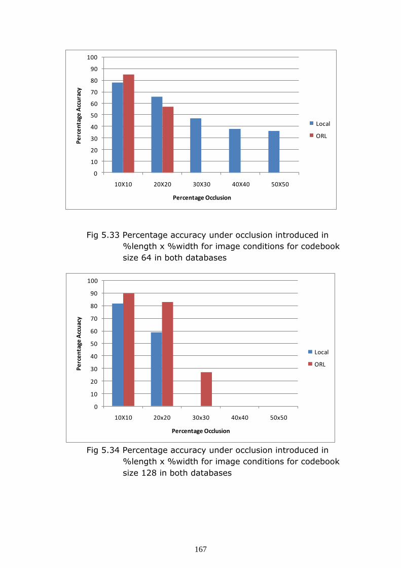
Fig 5.33 Percentage accuracy under occlusion introduced in
%length x %width for image conditions for codebook
size 64 in both databases
Fig 5.34 Percentage accuracy under occlusion introduced in
%length x %width for image conditions for codebook
size 128 in both databases
0
10
20
30
40
50
60
70
80
90
100
10X10 20X20 30X30 40X40 50X50
Pe
rce
nta
ge A
ccu
racy
Percentage Occlusion
Local
ORL
0
10
20
30
40
50
60
70
80
90
100
10X10 20x20 30x30 40x40 50x50
Pe
rce
nta
ge A
ccu
acy
Percentage Occlusion
Local
ORL

168
5.35 Percentage accuracy under occlusion introduced in
%length x %width for image conditions for codebook
size 256 in both databases
Observations: The graphs (Fig 5.32-Fig 5.53) show that as
occlusion increase on image the recognition accuracy reduces
drastically. The local database gives better accuracy and range
compared to ORL database for codebook size 64.
KFCG Results for various types of Noise
The KFCG algorithm for face recognition is tested for the various
types of noise introduced to the image like Speckle Noise, Salt and
pepper noise and Gaussian noise. Following are the graphs showing
in general performance of the KFCG algorithm for the various
codebook sizes.
0
10
20
30
40
50
60
70
80
90
100
10X10 20X20 30X30 40X40 50X50
Pe
rce
nta
ge A
ccu
racy
Percentage Occlusion
Local
ORL
169
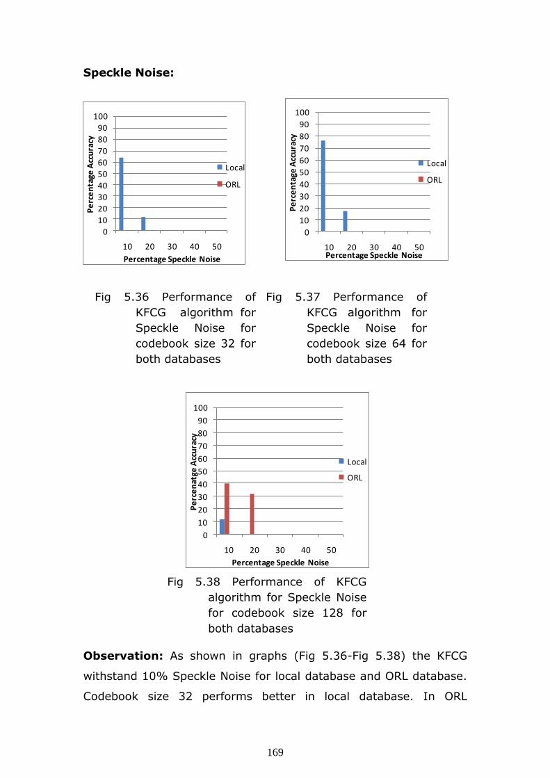
Speckle Noise:
Fig 5.36 Performance of
KFCG algorithm for
Speckle Noise for
codebook size 32 for
both databases
Fig 5.37 Performance of
KFCG algorithm for
Speckle Noise for
codebook size 64 for
both databases
Fig 5.38 Performance of KFCG
algorithm for Speckle Noise
for codebook size 128 for
both databases
Observation: As shown in graphs (Fig 5.36-Fig 5.38) the KFCG
withstand 10% Speckle Noise for local database and ORL database.
Codebook size 32 performs better in local database. In ORL
0
10
20
30
40
50
60
70
80
90
100
10 20 30 40 50
Pe
rce
nta
ge A
ccu
racy
Percentage Speckle Noise
Local
ORL
0
10
20
30
40
50
60
70
80
90
100
10 20 30 40 50
Pe
rce
nta
ge A
ccu
racy
Percentage Speckle Noise
Local
ORL
0
10
20
30
40
50
60
70
80
90
100
10 20 30 40 50
Pe
rce
nat
ge A
ccu
racy
Percentage Speckle Noise
Local
ORL

170
database only 128 codebook respond well to noise addition.
Codebook size 256 cannot withstand Speckle Noise addition in
either of the databases.
Gaussian Noise:
Fig 5.39 Performance of KFCG
algorithm for Gaussian
noise for codebook size
32 for both databases
Fig 5.40 Performance of KFCG
algorithm for Gaussian
noise for codebook size
64 for both databases
Fig 5.41 Performance of KFCG
algorithm for Gaussian
noise for codebook size
128 for both databases
Fig 5.42 Performance of KFCG
algorithm for Gaussian
noise for codebook size
256 for both databases
0102030405060708090
100
1 5 10
Pe
rce
nta
ge A
ccu
racy
Percentage Gaussian Noise
Local
ORL
0102030405060708090
100
1 5 10P
erc
en
tage
Acc
ura
cy
percentage Gaussian Noise
Local
ORL
0
10
20
30
40
50
60
70
80
90
100
1 5 10
Pe
rce
nta
ge A
ccu
racy
Percenatage Gaussian Noise
Local
ORL
0102030405060708090
100
1 5 10
Pe
rce
nta
ge a
ccu
racy
Percentage Gaussian Noise
Local
ORL

171
Observation: As shown in graphs (Fig 5.39-Fig 5.42) the KFCG
withstand 1% Gaussian noise addition for local database for
codebook size of 32. ORL database does not support noise addition
at all. As codebook size increases the ORL shows better
performance than local database.
Salt and Pepper Noise:
Fig 5.43 Performance of KFCG
algorithm for Salt and
Pepper noise for
codebook size 32 for
both databases.
Fig 5.44 Performance of KFCG
algorithm for Salt and
Pepper noise for codebook
size 64 for both databases.
Fig 5.45 Performance of KFCG
algorithm for Salt and
Pepper noise for codebook
size 128 for both databases
Fig 5.46 Performance of KFCG
algorithm for Salt and
Pepper noise for codebook
size 256 for both databases
0
10
20
30
40
50
60
70
80
90
100
10 20 30 40 50
Pe
rce
nta
ge A
ccu
racy
Percentage Salt & Pepper noise
Local
ORL
0
10
20
30
40
50
60
70
80
90
100
10 20 30 40 50
Pe
rce
nta
ge A
ccu
racy
Percentage Salt & Pepper Noise
Local
ORL
0
10
20
30
40
50
60
70
80
90
100
10 20 30 40 50
Pe
rce
nta
ge A
ccu
racy
Percentage Salt & Pepper Noise
Local
ORL
0
10
20
30
40
50
60
70
80
90
100
10 20 30 40 50
Pe
rce
nta
ge a
ccu
raac
y
Percentage Salt & Pepper Noise
Local
ORL

172
Observation: The graphs (Fig 5.43-Fig 5.46) shows Salt and
Pepper noise addition. This noise is not tolerated by codebook size
32 in ORL database and codebook size 256 in local database. The
codebook size 64 can withstand noise addition upto 10%. The
codebook size 128 withstands the noise addition up to 40% for ORL
database. Local database does not support noise addition beyond
10%
Table 5.3 is a overall performance table for the KFCG. The data
given for accuracy of algorithm is for various codebook sizes like 32,
64, 128, and 256. Under occlusion and noise addition conditions the
accuracy below 50% is not considered.
Table 5.3 Overall Performance of KFCG
Codebook 32 64 128 256
Database Local ORL Local ORL Local ORL Local ORL
Accuracy 86% 93% 87% 98% 93% 99% 95% 99%
% Occlusion withstand
50%X50% 50%X50% 50%X50% 50%X50% 50%X50% 50%X50% 50%X50% 50%X50%
Speckle Noise
10% 0% 10% 0% 10% 10% 0% 0%
Gaussian 1% 0% 0% 1% 0% 1% 0% 1%
Salt&
Pepper
0% 10% 10% 10% 20% 20% 10% 10%
The Table 5.3 shows overall performance of KFCG algorithm. The
ORL database due to its controlled nature performs better than local
database. This method strongly supports the occlusion introduced
on images. It is sensitive to noise addition but gives good result for
salt and pepper noise for codebook size 128 in both databases.
173
5.5 Summary
In this chapter the face recognition based on various VQ techniques
is studied for standard as well as locally created unconstrained
database. The newly suggested Kekre‘s Fast Codebook Generation
(KFCG) method gives better performance than LBG and K-Means.
As the codebook size increases the recognition accuracy improves
as well as algorithm becomes more robust against occlusion
condition. The smaller codebook size gives better performance for
noise addition conditions due to its larger size of cluster. LBG has
high FAR and K-Means has high FRR ratio but KFCG has good
discrimination power and gives zero FAR and FRR.


![QUANTIZATION TECHNIQUES - Shodhgangashodhganga.inflibnet.ac.in/bitstream/10603/25341/8/08... · 2018-07-09 · 3.3 VECTOR QUANTIZATION: Vector quantization [10, 11] is a process by](https://img.pdfslide.us/doc/110x75/5e5f8dd3f520f53a2949b994/quantization-techniques-2018-07-09-33-vector-quantization-vector-quantization.jpg)


![[CSCI 6990-DC] 09: Scalar Quantizationcmliu/Courses/Compression/... · 2009-04-27 · Vector Quantization (c.1) Vector quantization the vector quantization of x may be viewed as a](https://img.pdfslide.us/doc/110x75/5e5f90da59224a0df964048d/csci-6990-dc-09-scalar-quantization-cmliucoursescompression-2009-04-27.jpg)
![Compressing Unknown Images With Product …openaccess.thecvf.com/content_CVPR_2019/papers/Li...2.2. Vector Quantization Vector Quantization (VQ) [25] has been widely used in data compression](https://img.pdfslide.us/doc/110x75/5f35621b877e0f70241cbf60/compressing-unknown-images-with-product-22-vector-quantization-vector-quantization.jpg)