CHAPTER 4

Experimental Modeling

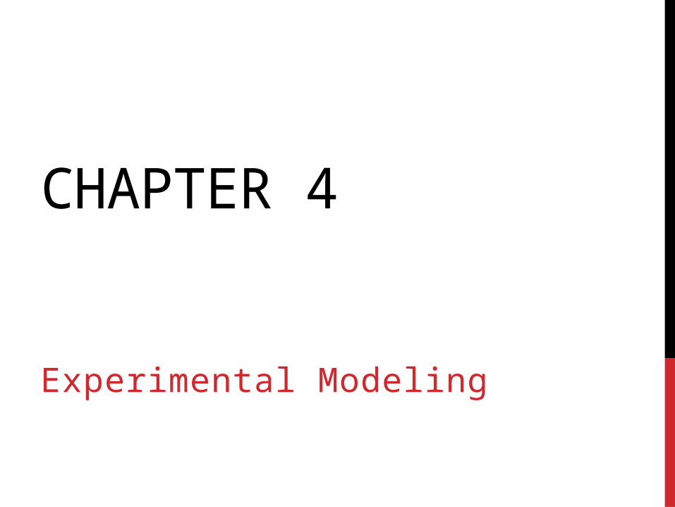
Introduction• Recall the difference between curve fitting and interpolation.

• In many cases the modeler is unable to construct a tractable model form that satisfactorily explains the behavior.

• The modeler may conduct experiments (or otherwise gather data) to investigate the behavior of the dependent variable(s) for selected values of the independent variable(s) within some range.

• With this information, the modeler can construct an empirical model based on the collected data rather than select a model based on certain assumptions.

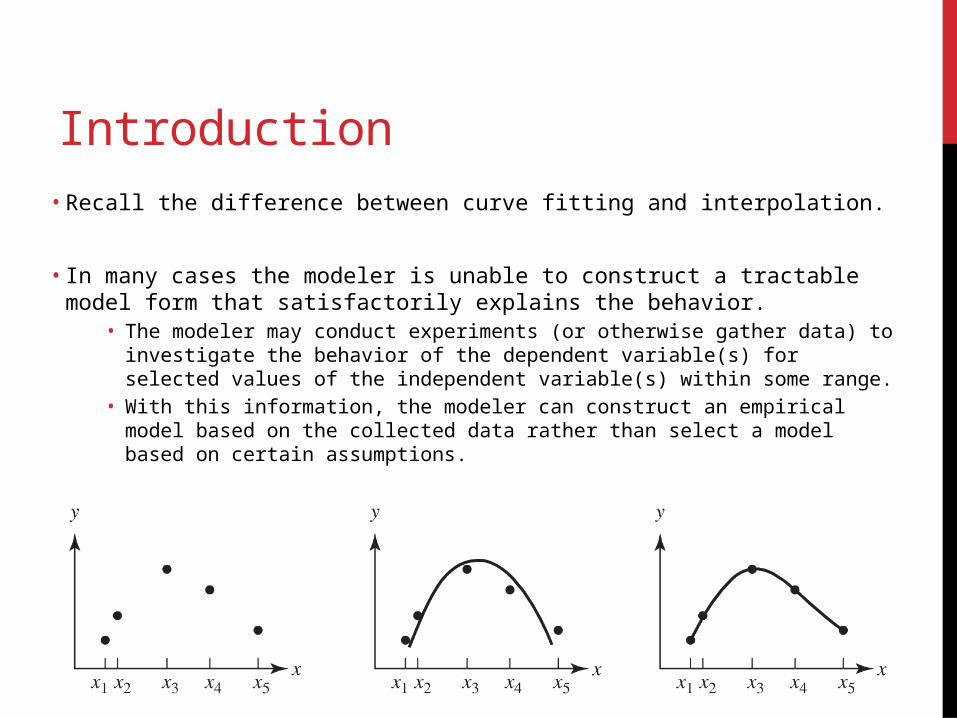
4.1 Harvesting in the Chesapeake Bay and Other One-Term Models

• Consider a situation in which a modeler has collected some data but is unable to construct an explicative model.

• Harvesting of bluefish and blue crabs versus time (the model may help to predict availability).

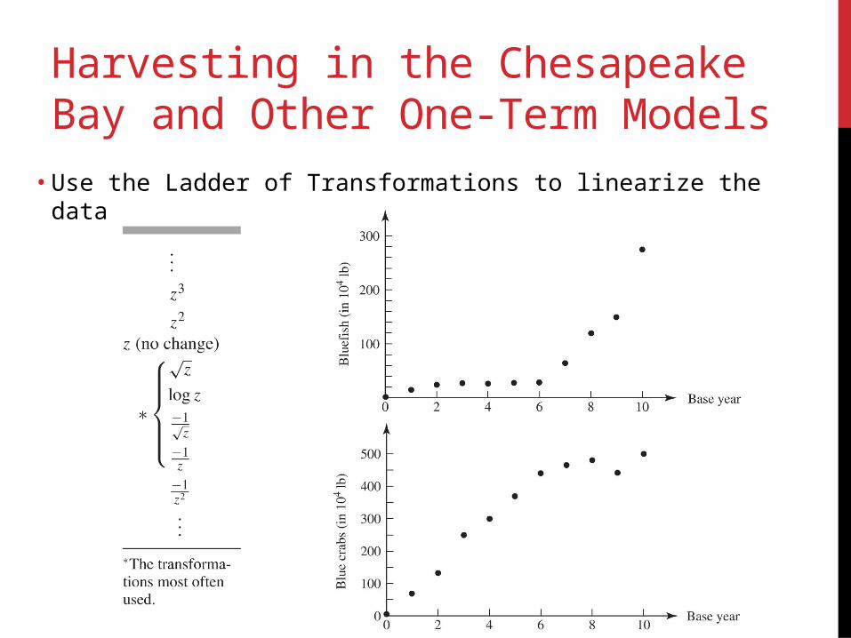
Harvesting in the Chesapeake Bay and Other One-Term Models

• Use the Ladder of Transformations to linearize the data

4.2 High-Order Polynomial Models

Polynomial Models

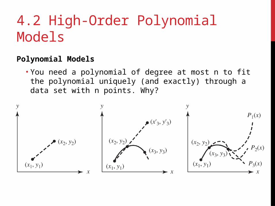
• You need a polynomial of degree at most n to fit the polynomial uniquely (and exactly) through a data set with n points. Why?

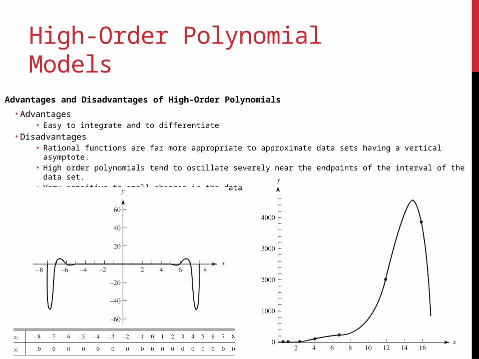
High-Order Polynomial ModelsAdvantages and Disadvantages of High-Order Polynomials

• Advantages• Easy to integrate and to differentiate

• Disadvantages• Rational functions are far more appropriate to approximate data sets having a vertical asymptote.• High order polynomials tend to oscillate severely near the endpoints of the interval of the data set.• Very sensitive to small changes in the data

4.4 Cubic Spline Models

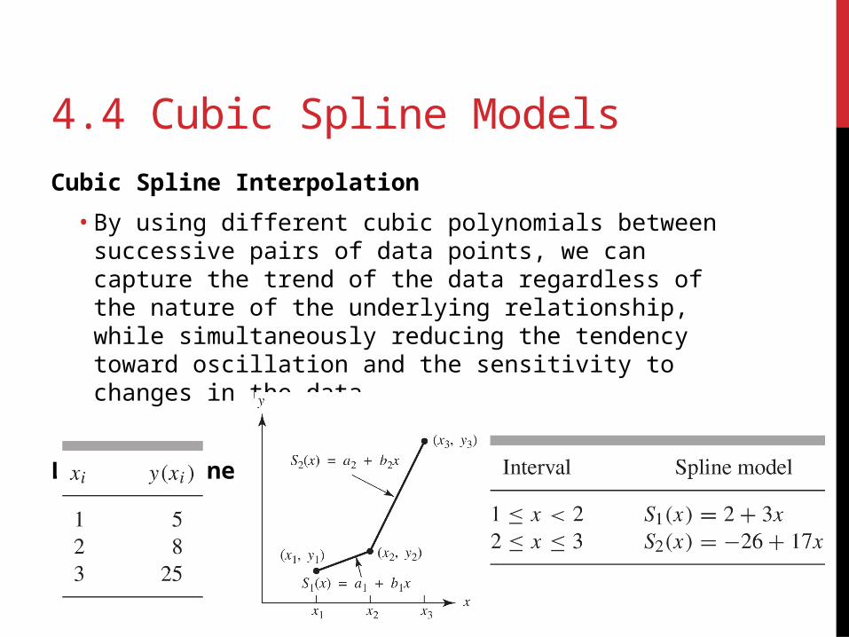
Cubic Spline Interpolation

• By using different cubic polynomials between successive pairs of data points, we can capture the trend of the data regardless of the nature of the underlying relationship, while simultaneously reducing the tendency toward oscillation and the sensitivity to changes in the data.

Linear Spline

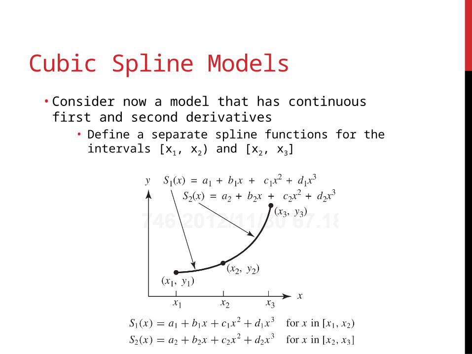
Cubic Spline Models• Consider now a model that has continuous first and second

derivatives• Define a separate spline functions for the intervals [x1, x2) and

[x2, x3]

Cubic Spline Models

Requirements

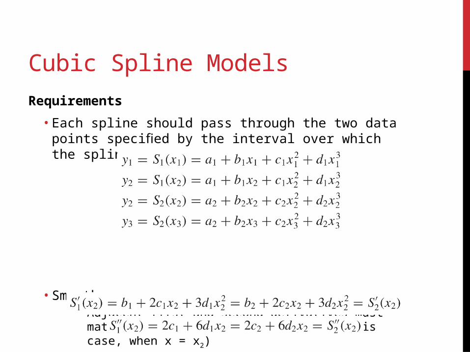
• Each spline should pass through the two data points specified by the interval over which the spline is defined.

• Smoothness• Adjacent first and second derivatives must match at the

interior data point (in this case, when x = x2)

Cubic Spline Models

Requirements

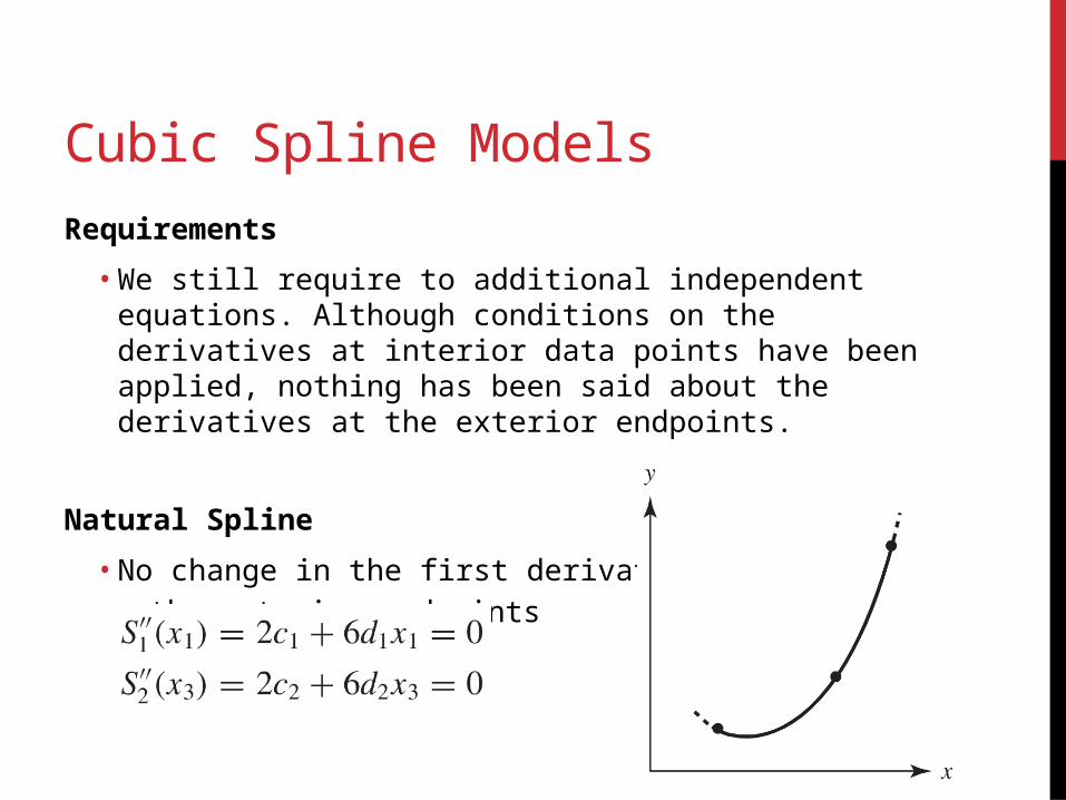
• We still require to additional independent equations. Although conditions on the derivatives at interior data points have been applied, nothing has been said about the derivatives at the exterior endpoints.

Natural Spline

• No change in the first derivative at

the exterior endpoints

Cubic Spline Models

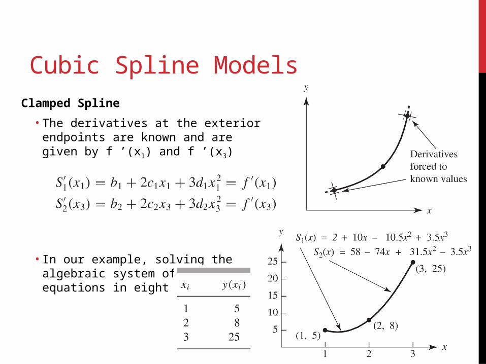
Clamped Spline

• The derivatives at the exterior endpoints are known and are given by f ’(x1) and f ’(x3)

• In our example, solving the algebraic system of eight equations in eight unknowns:

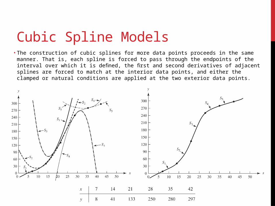
Cubic Spline Models• The construction of cubic splines for more data points proceeds in the same manner.

That is, each spline is forced to pass through the endpoints of the interval over which it is defined, the first and second derivatives of adjacent splines are forced to match at the interior data points, and either the clamped or natural conditions are applied at the two exterior data points.