Embed Size (px)
Citation preview
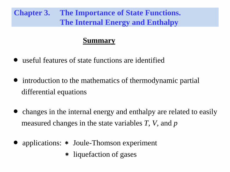
Chapter 3. The Importance of State Functions.
The Internal Energy and Enthalpy
Summary
useful features of state functions are identified
introduction to the mathematics of thermodynamic partial
differential equations
changes in the internal energy and enthalpy are related to easily
measured changes in the state variables T, V, and p
applications: Joule-Thomson experiment
liquefaction of gases

Partial Differential equations - the “language” of thermodynamics
(and many other branches of science and technology)
What are differential equations?
What are “partial” differential equations?
Why are differential equations important?
How can they be used?
What rules apply?
Section 3.1 Mathematical Properties of State Functions:
Partial Differential Equations

First … “Ordinary” Differential Equations
only one independent variable
Example: independent variable x in the function f(x) = 10x3 – 3x
derivative of f(x)
[ slope of f(x) plotted against x ]
integral of f(x)
“add up” the df differentials
[ gives the change in f(x) ]
x
xfxxf
x
xf
)()(
d
)(d
)(
)(
ddd
)(d)()(
b
a
b
a
xf
xf
x
x
ab fxx
xfxfxff
lim
x 0
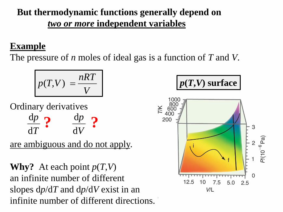
But thermodynamic functions generally depend on
two or more independent variables
Example
The pressure of n moles of ideal gas is a function of T and V.
Ordinary derivatives
are ambiguous and do not apply.
Why? At each point p(T,V)
an infinite number of different
slopes dp/dT and dp/dV exist in an
infinite number of different directions.
V
nRTT,Vp )(
V
p
T
p
d
d
d
d
p(T,V) surface
? ?

“Partial” Derivatives to the Rescue
For the derivatives of the function p(T,V), to avoid ambiguity,
define the partial derivatives:
lim
T 0 T
VTpVTTp
T
p
V
),(),(
V
VTpVVTp
V
p
T
),(),(lim
V 0
slope of p against T
parallel to the T axis
( V fixed )
slope of p against V
parallel to the V axis
( T fixed )
(Why “partial”? Only T and p are changing.)
(Only V and p are changing.)

Other Partial Differential Equations
1. Wave Equation
Vibration of an elastic string in one dimension:
u(x,t) is the displacement at time t and position x along the string.
c is the speed of the vibration moving along the string.
Three-dimensional vibration of an elastic medium (such as
sound waves, ultrasonic or seismic waves):
2
22
2
2
x
uc
t
u
ucz
uc
y
uc
x
uc
t
u 22
2
22
2
22
2
22
2
2

2. Heat Conduction Equation
Heat conduction in one dimension:
T(x,t) is the temperature at time t and position x.
k is the thermal conductivity.
Three-dimensional heat conduction:
2
2
x
Tk
t
T
Tkz
Tk
y
Tk
x
Tk
t
T 2
2
2
2
2
2
2
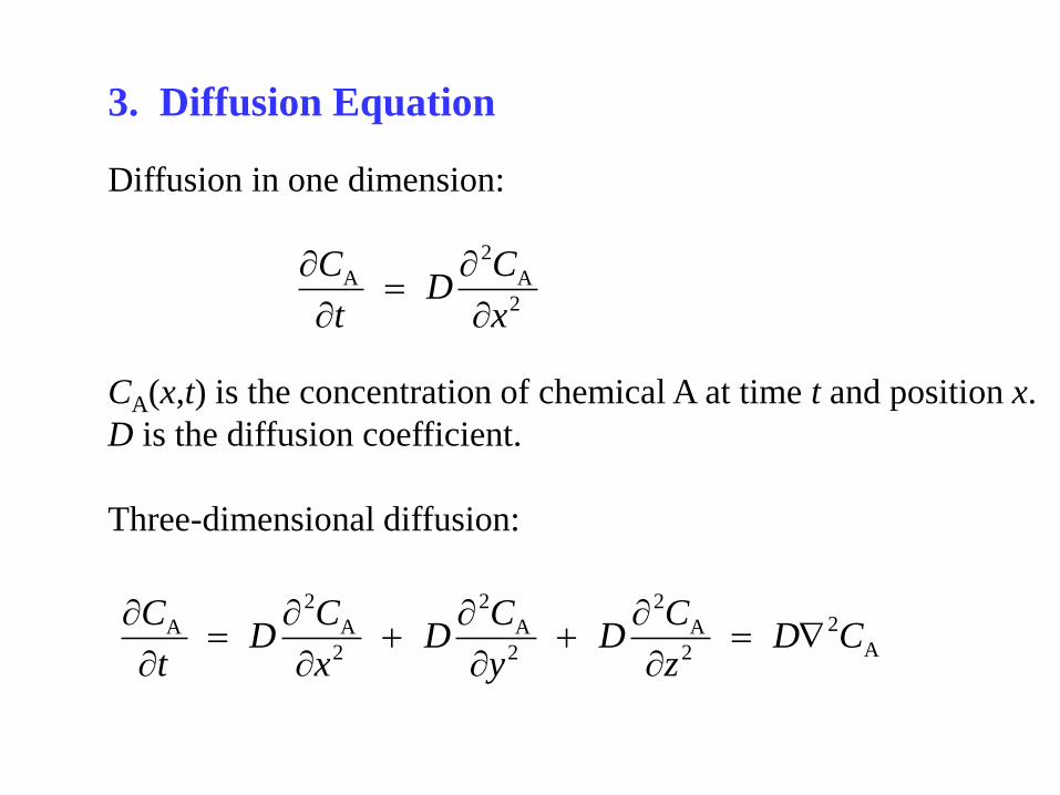
3. Diffusion Equation
Diffusion in one dimension:
CA(x,t) is the concentration of chemical A at time t and position x.
D is the diffusion coefficient.
Three-dimensional diffusion:
2
A
2
A
x
CD
t
C
A
2
2
A
2
2
A
2
2
A
2
A CDz
CD
y
CD
x
CD
t
C

4. Equation of Continuity for Fluid Flow
Fluid flow in one dimension:
(x,t) is the density of the fluid at time t and position x.
vx is the velocity of the fluid in the x direction.
Three-dimensional continuity equation:
xt
x
)v(
zyxt
zyx
)v()v()v(

5. Transmission Line Equation
Flow of electric current I(x,t) along a wire:
x is the position along the wire
R is the resistance
C is the capacitance
L is the induction
G is the loss
RGIt
IGLRC
t
ILC
x
I
)(
2
2
2
2

6. Lagrangian Equations of Motion
L = kinetic energy – potential energy for a mechanical system
qi is the generalized position of mass i (any coordinate system)
is the generalized velocity of mass i
ii q
L
q
L
t
d
d
iq

7. Schrodinger Quantum Mechanical Equation
h = Planck constant m = particle mass
V = potential energy = wave function
E = total energy
Solving the Schrodinger equation for an electron in the electric
potential energy field of a proton gives the 1s, 2s, 2p, 3s, …
orbitals used by chemists
EV
zyxm
h
2
2
2
2
2
2
2
2
8

partial T derivative:
partial V derivative:
T
p
V
nR
T
T
V
nR
T
VnRT
T
p
VVV
]/[
n,R,V constant
1
V
p
V
nRT
VnRT
V
VnRTV
VnRT
V
p
T
TT
2
2
11
]/[
n,R,T constantsame as d(1/V) / dV at fixed T
Example: Partial Derivatives of p(T,V) for an Ideal Gas

“Exact” Differential of p(T,V)
Because p is a function of state variables T and V:
a) the infinitesimal change in p (the differential dp) produced by
changes dT and dp is exactly defined (not path-dependent):
b) the change in p obtained by integrating dp is exactly defined
by the initial state pi(Ti, Vi) and the final state pf(Tf, Vf)
(also not path-dependent)
VV
pT
T
pp
TV
ddd
),(),(d
,
,
iiifff
VT
VT
VTpVTpppff
ii

Inverse Rule
Cyclic Rule
(why cyclic?)
Using the inverse rule, the cyclic rule is also written as:
V
V
p
TT
p
1
1
TpV p
V
V
T
T
p
pTV T
V
V
p
T
p
Buy two partial derivatives,
get one free!
Useful Rules for Partial Derivatives

Where Does the Cyclic Rule Come From?
VV
pT
T
pp
TV
ddd
divide by dT at constant p
(dp = 0)
pTpV T
V
V
p
T
T
T
p
d
d
d
d0
pTV T
V
V
p
T
p
)1(0
pTV T
V
V
p
T
p
Cyclic Rule
pTV T
V
V
p
T
p
:notice
Why the minus sign
in the Cyclic Rule?
At constant p, the
change in p caused by dT
cancels the change in p
caused by dV so that dp = 0.
Why? dV at constant T does
not equal dV at constant p.

Mixed Partial Derivatives: Order of Differentiation of a Function
Doesn’t Matter
Example:
Can be used as a test to show
is an exact differential.
Exercise For an ideal gas (p = nRT/V), verify:
VTTV V
p
TT
p
V
VTTV V
p
TV
nR
T
p
V
2
T first, then V V first, then T
VV
pT
T
pp
TV
ddd

Proof (a bit tricky)
VVT V
VTpVVTp
TV
p
T
),(),(lim
V 0
T
V
VTpVVTp
V
VTTpVVTTp ),(),(),(),(
lim
V 0
lim
T 0
V
T
VTpVTTp
T
VVTpVVTTp ),(),(),(),(lim
T 0lim
V 0
TT
VTpVTTp
V
),(),(lim
T 0
TVT
p
V

Useful and convenient (intensive) experimental quantities:
Volumetric Thermal Expansion Coefficient
Isothermal Compressibility ( also called T )
pT
V
V
1
gives the fractional
change in volume
per Kelvin
gives the negative
fractional change in
volume per Pa
is usually (but not always) positive.
Tp
V
V
1
(V/p)T is always negative, so is always positive.
Important Application: p-V-T Calculations

Note: for H2O(liquid) at 0 oC, = 5.47 105 K1 (shrinks when heated!)

Application of thermal expansion …
Liquid-in-Glass Thermometers
Liquid when heated
expands more than
the glass.
Related: Why can warm water
sometimes be used to get a
tight lid off a glass jar?
liquid > glass

Hot Rivet Fasteners
Hot rivet shrinks as it cools, tightly fastening two metal pieces.
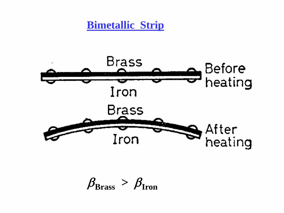
Bimetallic Strip
Brass > Iron
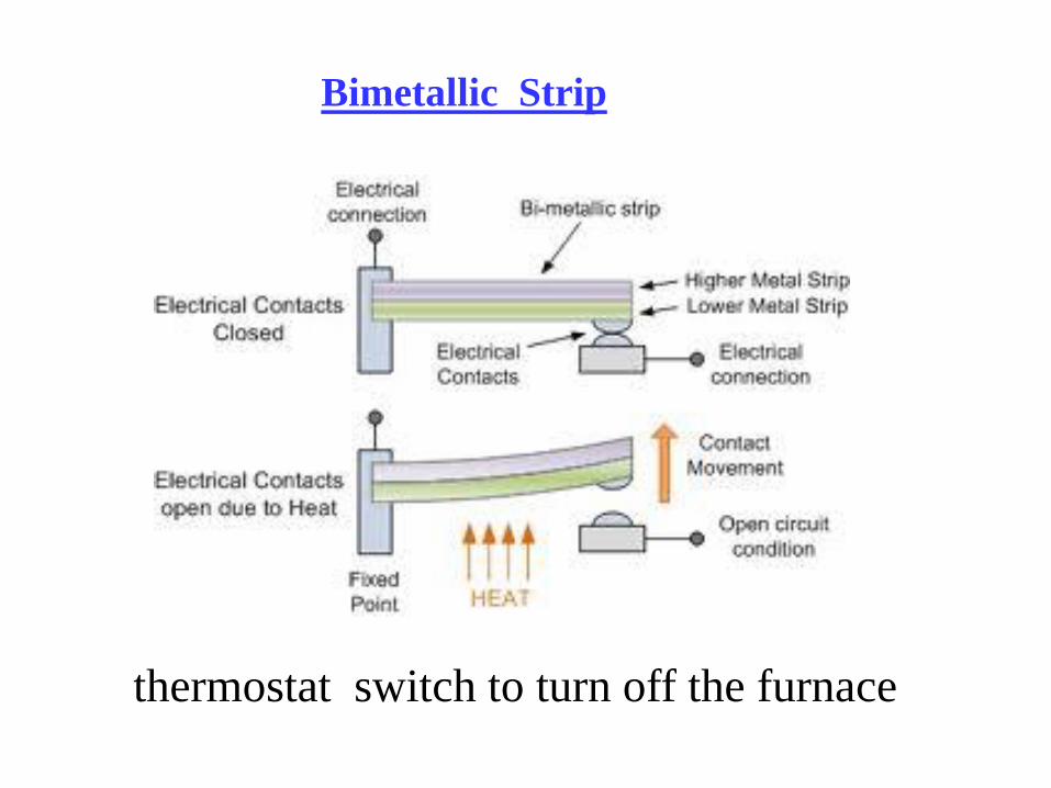
Bimetallic Strip
thermostat switch to turn off the furnace

fractional change in length per degree
Volumetric Thermal Expansion Coefficient
Linear Thermal Expansion Coefficient linear
pT
V
V
1 fractional change in volume per degree
3
1
3
11linear
pp T
V
VT
Can you
show this?
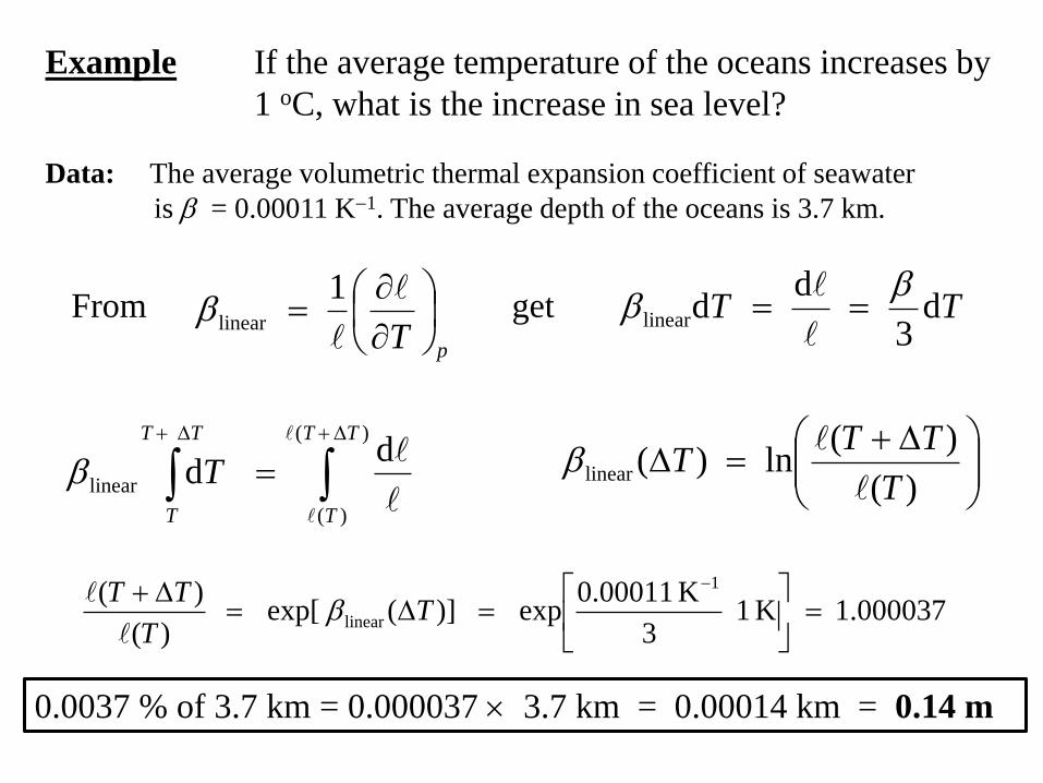
Example If the average temperature of the oceans increases by
1 oC, what is the increase in sea level?
Data: The average volumetric thermal expansion coefficient of seawater
is = 0.00011 K1. The average depth of the oceans is 3.7 km.
pT
1linearFrom get TT d
3
ddlinear
)(
)(
linear
dd
TT
T
TT
T
T
)(
)(ln)(linear
T
TTT
1.000037K13
K00011.0exp)](exp[
)(
)( 1
linear
TT
TT
0.0037 % of 3.7 km = 0.000037 3.7 km = 0.00014 km = 0.14 m

What’s this? What does it have to do with thermal expansion?

Concorde Supersonic (Mach 2.0) Passenger Aircraft
At cruising speed, twice the speed of sound, air friction heated the skin
to about 150 oC, increasing the length of the aircraft by about one foot, an
important design consideration for maintaining structural integrity.

Tp
V
V
1

How are and measured?
One way: measure the density (T,p) of a gas, liquid, or solid
at different temperatures and pressures.
(T,p) = mass per unit volume at temperature T, pressure p
Then use:
pp TT
V
V
11
TTpp
V
V
11
Can you derive the equations for and in terms of the density?
Are and intensive or extensive quantities?

Exercise: Evaluate the volumetric thermal expansion coefficient
for an ideal gas (V = nRT/p) at 298 K
1K 00335.0K298
1
1
1
1
1
TnRT
nR
pV
nR
T
T
p
nR
V
p
nRT
TV
T
V
V
p
p
p
T
1
gas ideal

Exercise: Evaluate the isothermal compressibility
for an ideal gas (V = nRT/p) at p = 1.00 bar
1
2
1
bar00.1bar00.1
1
111
1
1
1
pppV
nRT
pV
nRT
p
pnRT
V
p
nRT
pV
p
V
V
T
T
T
p
1
gas ideal

Exercise: For a nonideal gas with second virial coefficient B(T)
and the equation of state
show that the isothermal compressibility is
V
TnB
nRT
pVZ
)(1
2
m2
2 )(
1
)(
1
V
TRTBp
V
TRTBnp

Isothermal Compressibility of a Nonideal Gas
with Second Virial Coefficient B(T)
2
m2
2 )(
1
)(
1
V
TRTBp
V
TRTBnp
Significance:
ideal gas with B(T) = 0 no molecular interactions
________________________________________________________________________________________________________________________________________________________________
nonideal gas with B(T) < 0 attractive interactions dominate
gas is “more compressible”_________________________________________________________________________________________________________________________________________________________________
nonideal gas with B(T) > 0 repulsive interactions dominate
gas is “less compressible”
= 1/p
> 1/p
< 1/p
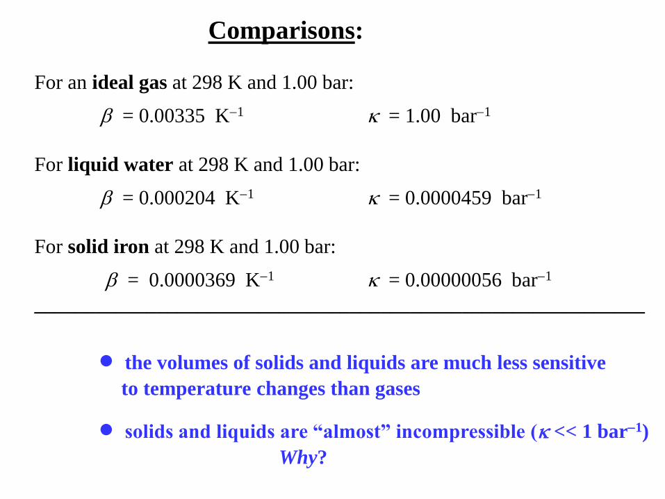
Comparisons:
For an ideal gas at 298 K and 1.00 bar:
= 0.00335 K1 = 1.00 bar1
For liquid water at 298 K and 1.00 bar:
= 0.000204 K1 = 0.0000459 bar1
For solid iron at 298 K and 1.00 bar:
= 0.0000369 K1 = 0.00000056 bar1
____________________________________________________________
the volumes of solids and liquids are much less sensitive
to temperature changes than gases
solids and liquids are “almost” incompressible ( << 1 bar1)
Why?

Exercise: 2.00 L of ideal gas at 298 K (25 oC) and 1.00 bar is
heated at constant pressure to 323 K (50 oC). Calculate the
final volume.
Easy! The equation of state pV = nRT is known. Use:
Vf / Vi = (nRTf /pf) / (nRTi /pi) = Tf / Ti = (323 K / 298 K) = 1.0839
Vf = 1.0839 2.00 L
Vf = 2.17 L
increase volume%5.8
%100L00.2
L00.2L17.2%100change volume%
i
if
V
VV

Exercise: 2.00 L of liquid water at 298 K (25 oC) and 1.00 bar is
heated at constant pressure to 323 K (50 oC). Calculate the
final volume. Data: = 0.000204 K1 (assumed constant).
Note: The equation of state of liquid water is not provided.
Can’t use pV = nRT (liquid H2O is not an ideal gas). Instead:
TV
Vf
i
f
i
T
T
V
V
dd
pT
V
V
1 T
V
dVd dTp
0051.0)K25(K000204.0)(ln 1
if
i
fTT
V
V
0051.1e 0051.0 i
f
V
V Vf = 1.0051 Vi = 1.0051 2.00 L
Vf = 2.01 L (only a 0.5 % increase)
Integrate at constant pressure:

Exercise: 2.00 L of ideal gas at 298 K (25 oC) and 1.00 bar is
isothermally compressed to a final pressure of 5.00 bar.
Calculate the final volume.
Easy! The equation of state pV = nRT is known. Use:
Vf / Vi = (nRTf /pf) / (nRTi /pi) = pi / pf = (1.00 bar / 5.00 bar) = 0.200
Vf = 0.200Vi = 0.200 2.00 L
Vf = 0.400 L
%0.80
%100L00.2
L00.2L400.0%100change volume%
i
if
V
VV
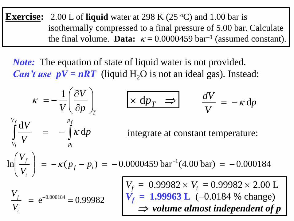
Exercise: 2.00 L of liquid water at 298 K (25 oC) and 1.00 bar is
isothermally compressed to a final pressure of 5.00 bar. Calculate
the final volume. Data: = 0.0000459 bar1 (assumed constant).
Note: The equation of state of liquid water is not provided.
Can’t use pV = nRT (liquid H2O is not an ideal gas). Instead:
pV
Vf
i
f
i
p
p
V
V
dd
Tp
V
V
1 p
V
dVd dpT
000184.0bar)00.4(bar0000459.0)(ln 1
if
i
fpp
V
V
99982.0e 000184.0
i
f
V
VVf = 0.99982 Vi = 0.99982 2.00 L
Vf = 1.99963 L (0.0184 % change)
volume almost independent of p
integrate at constant temperature:

VT
p
Railroads are constructed with small gaps between lengths of
steel rails to allow for thermal expansion
Bridges have small gaps between structural beams
Liquid-in-glass thermometers break if heated beyond their
temperature range
Never fill a container to the brim with a liquid and seal it!
Useful application: “shrink fits” used by machinists
What does thermodynamics have to say about ?
!!! Warning !!!Heating a solid or a liquid at constant volume can
produce dangerously large pressure increases.

Thermal Expansion Gaps

No Thermal Expansion Gaps!

Change in Pressure with Temperature at Constant Volume
pTV T
V
V
p
T
p
T
p
p
V
T
V
T
p
p
V
V
T
V
V
1
1
ratio of the volumetric thermal expansion
coefficient to the isothermal compressibility
Cyclic Rule!
Inverse Rule!
Definition of ,

Changes in Pressure with Temperature at Constant Volume
1Kbar00335.0K298
bar00.1
1
1
T
p
p
T
T
p
V
For an ideal gas at 298 K and 1 bar:
For solid iron at 298 K and 1 bar:
1
1
1
Kbar66bar00000056.0
K0000369.0
VT
p
970 lb per square inch per degree ! Uh Oh!
(no problem)

Freezing liquid water in a confined space can split pipes,
damage concrete, heave foundations, and crack porous rocks.
Why ?

Exercise: Liquid water at 0 oC and 1.00 bar is frozen
at constant volume. Calculate the final pressure.
Data: Ice is less dense than liquid water. (Ice floats!) Freezing
liquid water produces a 9 % increase in volume.
isothermal compressibility of ice = 51.0 106 bar1
Solution: Freezing water at 1.00 bar increases the volume by 9 %.
To maintain constant volume, the pressure on the
ice must be increased to reduce the volume by 9 %.
Tp
V
V
1
V
dVp d
multiply by dp at constant T
integrate from pi = 1.00 bar to pf

Exercise: Liquid water at 0 oC and 1.00 bar is frozen at
constant volume. Calculate the final pressure.
f
i
f
i
f
i
V
V
p
p
p
pV
dVpp dd
(cont.)assume is constant
(no other information given)
i
f
ifV
Vpp ln)(
i
f
ifV
Vpp ln
1
09.1
1ln
bar100.51
1bar00.1
16fp
bar1700bar1690bar00.1 fp
Conclusion: Freezing liquid water at constant volume
generates a pressure of about 1700 bar
( 25,000 lb per square inch! Uh Oh!)

Sections 3.2 and 3.3 Dependence of the Internal Energy U
on Temperature and Volume
widely used for scientific and engineering calculations
provides valuable information about molecular energy levels
and molecular interactions
Because the internal energy of a system is a state function U(T,V),
the differential dU is exact. Mathematics provides:
VV
UT
T
UU
TV
ddd
A useful theoretical result. But for practical applications:
How are (U/T)V and (U/V)T calculated ?

(U/T)V
from the First Law: dU = dq + dw
only p-V work possible: dU = dq pexternaldV
at constant volume: dUV = dqV
(dV = 0, no work)
V
VV
T
U
T
qC
d
d
???
heat capacity at
constant volume
CV is an experimental quantity, measured using calorimetry.

(U/V)T
from Chapters 1 and 2:
???
Plan A If the equation of state of the system is known, then
(p/T)V and therefore (U/V)T are easily calculated.
Plan B If the equation of state of the system is unknown, then
(p/T)V and (U/V)T can be calculated using measurable
volumetric thermal expansion coefficients () and isothermal
compressibilities () (see Section 3.1) using
pT
pT
V
U
VT
VT
ppT
V
U
T

So What
Important result: Changes in the internal energy of any system
can be calculated from measurable quantities.
???
Tp
VV
p
V
VT
V
VT
qC
11
d
d
VV
UT
T
UU
TV
ddd
“theoretical”
becomes “practical”
in terms of the measurable quantities:
VpTTCU V ddd

Exercise: For ideal gases, prove 0
TV
U
Hint: Recall that the volumetric expansion coefficient and isothermal
compressibility of an ideal gas are = 1/T and = 1/p_________________________________________________________
Exercise: Theory is fine, but can you suggest an experiment that
could be used to show (U/V)T = 0 for ideal gases?
One possibility:
Open a valve, allow gas at
pressure pi in flask A to expand
into evacuated flask B.
If the gas is ideal, what is the
change in temperature?
Why?

Sections 3.4 to 3.6 Dependence of the Enthalpy H = U + pV
on Temperature and Pressure
recall from Chapter 2: qp = H
as a result, enthalpy changes are important for calorimetry,
combustion reactions and other chemical reactions
also important for flow processes (next Section)
T and p are therefore “natural” variables for the enthalpy.
H is a state function H(T,p), so the differential dH is exact and
pp
HT
T
HH
Tp
ddd
Another useful theoretical result. But for practical applications
how are (H/T)p and (H/p)T calculated ?

(H/T)p
from the First Law: dU = dq + dw
only p-V work possible: dU = dq pexternaldV
at constant pressure: dUp = dqp pdV
dqp = dUp + pdV = d(U + pV)
= dH
p
p
pT
H
T
qC
d
d
?
heat capacity at
constant pressure
Cp is an experimental quantity measured using calorimeters
operated at constant pressure

(H/p)T ?
VVT
Vp
VT
p
H
TT
dH = d(U + pV)
= dU + d(pV)
= dU + pdV + Vdp
= (U/T)V dT + (U/V)T dV + pdV + Vdp
= CVdT + [T(p/T)V – p]dV + pdV + Vdp
dHT = T(/)dVT + VdpT ( dT = 0 at constant T, divide by dpT )
)1( TVp
H
T
V, , and T are all measurable quantities
/

So What
Important result: Changes in the enthalpy of any system
can be calculated from measurable quantities.
???
p
p
pT
V
VT
qC
1
d
d
pp
HT
T
HH
Tp
ddd
“theoretical”
becomes “practical”
in terms of the measurable quantities:
pTVTCH p d)1(dd

Exercise: For ideal gases, show
As a result, the enthalpy of an ideal gas depends
only on temperature and
dH = CpdT (even if p is changing!)
0
Tp
H
Exercise: For liquids and solids, show
As a result
dH CpdT + Vdp (liquids and solids)
Vp
H
T

Example Problem 3.9
Calculate the change in enthalpy when 124 g of liquid methanol at
1.00 bar and 298 K is heated and compressed to 2.50 bar and 425 K .
Data: methanol molar mass M = 32.04 g mol1
density of liquid methanol = 0.791 g cm3
heat capacity of liquid methanol Cpm = 81.1 J K1 mol1
Solution:
Enthalpy is a state function, so H can be calculated for any path
between the initial and final states. We will heat first, then compress:
CH3OH(298 K, 1 bar) CH3OH(425 K, 1 bar) CH3OH(425 K, 2.50 bar)
compressheat
Step 1 Step 2

Example Problem 3.9 (cont.)
Step 1 Heat 124 g of liquid methanol from 289 K to 425 K at 1 bar.
Step 2 Compress 124 g of liquid methanol from 1.00 bar to 2.50 bar
at a constant temperature of 425 K.
)(dd mm ifp
T
T
p
T
T
pp TTnCTnCTCHf
i
f
i
J900,39)K298K425()molKJ1.81(molg04.32
g124 11
1
pH
)(ddd if
T
T
T
T
p
p T
T ppVpVpVpp
HH
f
i
f
i
f
i
J9.39)bar Pa10)(bar00.150.2)(cmm10)(cm g791.0/g124( 153363
TH
Overall H = Hp (step 1) + HT (step 2)
= 39,900 J + 40 J
39,900 J from step 1
For solids and liquids,
changes in pressure
usually cause small
enthalpy changes

Section 3.7 The Joule-Thomson (JT) Experiment
irreversible expansion of gas through a porous barrier or
throttle valve under adiabatic conditions (no heat flow)
ideal gases: no temperature change
real gases: can cool down or warm up during JT expansion
important applications refrigeration
air conditioning
heat pumps
gas liquefaction

Gas Liquefaction
For industrial applications:
(not university lab experiments!)
continuous flow (more
economical than batch
processing)
re-cycle gas that does
not liquefy (no wastage)
heat-exchange – use cool gas
that does not liquefy to pre-cool
gas from compressor
large-scale production
(thousands of tons per day)
use the expanding gas to run a
generator (adiabatic cooling)
Applications of Liquefied Gases
liquid air is distilled to produce liquid N2 and liquid O2
N2 is used to make ammonia for the production of nitric acid,
fertilizers, explosives, and many other industrial chemicals
cold liquefied natural gas (LNG) can be shipped economically
over large distances in cheap low-pressure tanks (at 1 atm)
liquid N2 and liquid He are important cryogens
(liquid He is used to operate superconducting nmr magnets)
liquid propane allows barbecuing without charcoal
many other important uses

Refrigeration and Air Conditioning
expanding nonideal gases cool and absorb heat
keeps perishable food products fresh, nutritious and safe to eat
Ever tried working (or living)
at 30 oC and 95 % humidity?
air conditioners provide cooling and humidity reduction, making
large regions “habitable” for “modern” people

LNG Ship Carrying Liquefied Natural Gas (at about 260 oC)

most powerful rocket ever built
operational 1967 to 1973
7.6 million pounds thrust
launched 130-ton payloads into earth orbit
never failed, even when hit by lighting (Apollo 12 mission)
kerosene / liquid oxygen first stage
liquid hydrogen / liquid oxygen second and third stages
mileage: about five inches per gallon
Application of Liquefied Gases:
Space Exploration
store liquid fuel and oxidizer in
light thin-wall low pressure tanks
Saturn V Heavy-Lift Vehicle
(“Apollo Moon Rocket”)

Joule Thomson (JT) Flow Experiment – How does it work?
gas initially at p1, V1, T1
expands adiabatically through a porous plug or throttle valve
gas downstream leaves at p2, V2, T2
work p1V1 done
on the gas to force
it through the plug
work p2V2 done
on the surroundings
by the expanding gas

Thermodynamic Analysis of Joule-Thomson (JT) Expansions
p1, V1, T1 p2, V2, T2
First Law: U = q + w
U2 U1 = p1V1 p2V2
U2 + p2V2 = U1 + p1V1
H2 = H1
H = 0
Conclusion: Joule-Thomson expansions are “isenthalpic”
(occur at constant enthalpy)
0

Joule-Thomson Coefficient of Performance
JT gives the change in temperature per unit change in pressure
of the expanding gas. But what is JT ?
Using the cyclic and inverse rules of partial derivatives:
Hp
T
JT
pTTpHT
H
p
H
p
H
H
T
p
T
JT
V(1 T) Cp
pC
TV )1(JT
Gives temperature change of the expanding
gas in terms of measurable quantities.

Hp
T
JT
JT > 0: expanding gas cools down
T < 0 if p < 0
JT < 0: expanding gas warms up
T > 0 if p < 0
Which of the listed substances would
make the best refrigerant? Why?

For an ideal gas (pV = nRT), recall
which gives (ideal gas)
pC
TV )1(JT
TT
V
V p
11
0)
11(
JT
pC
TT
V
Conclusion: Warming or cooling during Joule-Thomson expansions
occurs only for nonideal gases (molecular interactions).
Exercise: Evaluate the Joule-Thomson coefficient JT for
an ideal gases.

Why Does Warming or Cooling Occur During JT Expansions?
For a nonideal gas obeying the van der Waals equation
with attractive a and repulsive b coefficients
2
2
V
an
nbV
nRTp
the Joule-Thomson coefficient is
b
RT
a
Cp
JT
21
m

Joule-Thomson Coefficient of a Nonideal van der Waals Gas
b
RT
a
Cp
T
pH
JT
21
m
Low Temperatures: (2a/RT) – b > 0 JT > 0
Cooling on Expansion. Attractive forces dominate.
“Sticky” molecules fly apart more slowly, with less kinetic energy.
High Temperatures: (2a/RT) – b < 0 JT < 0
Warming on Expansion. Repulsive forces dominate.
Repelling molecules fly apart more quickly, with more kinetic energy.
Max. Inversion temperature: (2a/RT) – b = 0 JT = 0
No temperature change. Attractive and repulsive forces balanced at
the Boyle (not Boil!) temperature TBoyle = 2a/Rb.

Isenthalps: States of Constant Enthalpy
JT
Hp
T
Boyle temperature
(max. inversion temp.)
isenthalp slope:
(JT coefficient)
cooling
warming on
expansion
JT > 0
JT < 0
JT = 0
Graphical interpretation
of the Joule-Thomson
coefficient:

Joule-Thomson Inversion Temperatures for N2 and H2
cooling
warmingUse liquid N2 to
cool liquid H2
below its inversion
temperature.
Then use liquid H2
to cool and liquefy He.
Liquid helium is the
ultimate cryogen.
Used for super-conducting
magnets and low-temperature
research (T < 4 K).