33

CHAPTER 3

SOFTWARE USED

3.1 INTRODUCTION

In this work, all the analyses namely Forward Kinematics Analysis

(FKA), Reachability Analysis (RA), Path Analysis (PA), Workspace Analysis

(WA), and Inverse Kinematics Analysis (IKA) are done using LabVIEW and

FKM is verified using RoboCell and validated with AutoCAD. The

LabVIEW is much suitable for these analyses. Various features of the

software used and the reason for selecting the same are presented here as an

overview.

3.2 LABVIEW

In this research FKM, Reachability analysis, path and workspace

analyses, and IKM have been developed using LabVIEW. The LabVIEW is

employed for the analysis of SCORBOT ER V Plus. It has many tools and

they are efficiently used by many researchers. The reasons for using

LabVIEW in this research work are given below:

1. Dataflow Programming

2. Graphical Programming

3. Interfacing

4. Code compilation

5. Large libraries

34

6. Code re-use

7. Parallel programming

8. Ecosystem

3.2.1 Dataflow Programming

The programming language used in LabVIEW, also referred to as

G, is a dataflow programming language. Execution is determined by the

structure of a graphical block diagram (the LabVIEW-source code) on which

the programmer connects different function-nodes by drawing wires. These

wires propagate variables and any node can execute as soon as all its input

data become available. Since this might be the case for multiple nodes

simultaneously, G is inherently capable of parallel execution. Multi-

processing and multi-threading hardware is automatically exploited by the

built-in scheduler, which multiplexes multiple OS (Operating Systems)

threads over the nodes ready for executions.

3.2.2 Graphical Programming

LabVIEW ties the creation of user interfaces (called front panels)

into the development cycle. LabVIEW programs/subroutines are called VIs

(Virtual Instruments). Each VI has three components: a block diagram, a front

panel and a connector panel. The last is used to represent the VI in the block

diagrams of other, calling VIs. Controls and indicators on the front panel

allow an operator to input data into or extract data from a running virtual

instrument. However, the front panel can also serve as a programmatic

interface. Thus a virtual instrument can either be run as a program, with the

front panel serving as a user interface, or, when dropped as a node onto the

block diagram, the front panel defines the inputs and outputs for the given

node through the connector panel. This implies each VI can be easily tested

before being embedded as a subroutine into a larger program.

35

The graphical approach also allows non-programmers to build

programs by dragging and dropping virtual representations of lab equipment

with which they are already familiar. The LabVIEW programming

environment, with the included examples and documentation, makes it simple

to create small applications. This is a benefit on one side, but there is also a

certain danger of underestimating the expertise needed for high-quality G

programming. For complex algorithms or large-scale code, it is important that

the programmer possesses an extensive knowledge of the special LabVIEW

syntax and the topology of its memory management. The most advanced

LabVIEW development systems offer the possibility of building stand-alone

applications. Furthermore, it is possible to create distributed applications,

which can be communicated by a client/server scheme, and are therefore

easier to implement due to the inherently parallel nature of G.

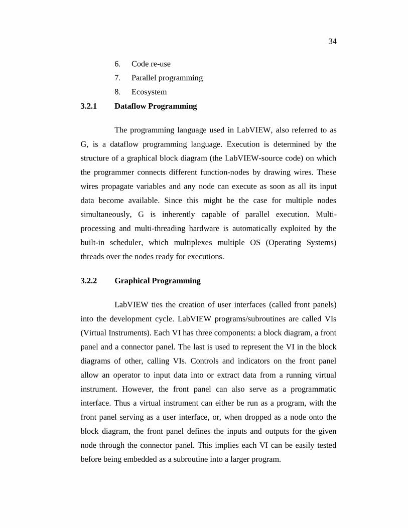
Figure 3.1 Screenshot of a simple LabVIEW Program

36

The image shown in Figure 3.1 is an illustration of a simple

LabVIEW program showing the dataflow source code in the form of the block

diagram in the lower left frame and the input and output variables as graphical

objects in the upper right frame. The two are the essential components (front

panel and block diagram) of a LabVIEW program referred to as a Virtual

Instrument.

3.2.3 Interfacing

A key benefit of LabVIEW over other development environments

is the extensive support for accessing instrumentation hardware. Drivers and

abstraction layers for many different types of instruments and buses are

included or are available for inclusion. These present themselves as graphical

nodes. The abstraction layers offer standard software interfaces to

communicate with hardware devices. The provided driver interfaces save

program development time. People even with limited coding experience can

write programs and deploy test solutions in a reduced time frame when

compared to more conventional or competing systems. A new hardware

driver topology (DAQmxBase), which consists mainly of G-coded

components with only a few register calls through NI Measurement Hardware

DDK (Driver Development Kit) functions, provides platform independent

hardware access to numerous data acquisition and instrumentation devices.

The DAQmxBase driver is available for LabVIEW on Windows, Mac OS X

and Linux platforms.

Although it is not a .NET language, LabVIEW offers an interface to

.NET Framework assemblies that make it possible to use, for instance,

databases and XML (Extensible Markup Language) files in automation

projects.

37

3.2.4 Code Compilation

In terms of performance, LabVIEW includes a compiler that

produces native code for the CPU (Central Processing Unit) platform. The

graphical code is translated into executable machine code by interpreting the

syntax and by compilation. The LabVIEW syntax is strictly enforced during

the editing process and compiled into the executable machine code when

requested to run or upon saving. In the latter case, the executable and the

source code are merged into a single file. The executable runs with the help of

the LabVIEW run-time engine, which contains some precompiled code to

perform common tasks that are defined by the G language. The run-time

engine reduces compile time and also provides a consistent interface to

various operating systems, graphic systems, hardware components, etc. The

run-time environment makes the code portable across platforms. Generally,

LabVIEW code can be slower than equivalent compiled C code, although the

differences often lie more with program optimization than inherent execution

speed.

3.2.5 Large Libraries

Many libraries with a large number of functions for data

acquisition, signal generation, mathematics, statistics, signal conditioning,

analysis, etc., along with numerous graphical interface elements are provided

in several LabVIEW package options. The number of advanced mathematic

blocks for functions such as integration, filters, and other specialized

capabilities usually associated with data capture from hardware sensors is

immense. In addition, LabVIEW includes a text-based programming

component called MathScript with additional functionality for signal

processing, analysis and mathematics. MathScript can be integrated with

graphical programming using "script nodes" and uses a syntax that is

generally compatible with MATLAB.

38

3.2.6 Code Re-use

The fully modular character of LabVIEW code allows code reuse

without modifications: as long as the data types of input and output are

consistent, two sub VIs are interchangeable. The LabVIEW professional

development system allows creating stand-alone executables and the resultant

executable can be distributed infinite times. The run-time engine and its

libraries can be provided freely along with the executable.

A benefit of the LabVIEW environment is the platform independent

nature of the G code, which is (with the exception of a few platform-specific

functions) portable between the different LabVIEW systems for different

operating systems (Windows, Mac OS X and Linux).

3.2.7 Parallel Programming

With LabVIEW it is very easy to program different tasks that are

performed in parallel by means of multithreading. This is, for instance, easily

done by drawing two or more parallel while loops. This is a great benefit for

test system automation, where it is a common practice to run processes like

test sequencing, data recording, and hardware interfacing in parallel.

3.2.8 Ecosystem

Due to the longevity and popularity of the LabVIEW language, and

the ability for users to extend the functionality, a large ecosystem of third

party add-ons has been developed through contributions from the community.

This ecosystem is available on the LabVIEW Tools Network, and is a

marketplace for both free and paid LabVIEW add-ons.

39

3.3 ROBOCELL

The RoboCell Software is used to validate the FKM in Stage I and

for path analysis in Stage II.

3.3.1 Components of RoboCell

RoboCell is a software package that integrates four components:

1. SCORBASE, a full-featured robotics control software package,

which provides a user-friendly tool for robot programming and

operation.

2. A Graphic Display module that provides 3D simulation of the

robot and other devices in a virtual robotic workcell where one

can define (teach) robot positions and execute robot programs.

3. CellSetup, which allows a user to create a new virtual robotic

workcell, or modify an existing workcell.

4. 3D Simulation Software Demo to demonstrate RoboCell’s

capabilities.

RoboCell’s representation of robot and devices is based on actual

dimensions and functions of SCORBOT equipment. Thus, operating and

programming the robot in RoboCell can be used with an actual robotic

installation. Graphic display features and automatic operations, such as Cell

Reset and Send Robot commands, enable quick and accurate programming.

RoboCell’s user interface and menus are similar to those of SCORBASE.

SCORBASE operations, menus and commands are described in the

SCORBASE User Manual.

40

3.3.2 Defining robot positions

RoboCell provides the methods described below for defining robot

positions. A position is identified by its assigned number.

3.3.2.1 Recording position (First method)

1. The SCORBASE Manual Movement dialog box is used to

manipulate the virtual robot in the same manner in which one

would manipulate an actual robot.

2. When the position is reached, a number is typed in the position

number field in the Teach Position (Simple) dialog box.

3. Record button is clicked.

If the position number has been used previously, the new position will

overwrite the previous position data.

3.3.2.2 Recording Position (Second method)

1. To send a robot to a required position, the “Send Robot to

Object/Position/Above Position” tools are used.

2. The Manual Movement dialog box is used for fine-tuning.

3. When the position is reached, a number in the position number

field in the Teach Position (Simple) dialog box is typed.

4. Record button is clicked.

If the position number has been used previously, the new position will

overwrite the previous position data.

41

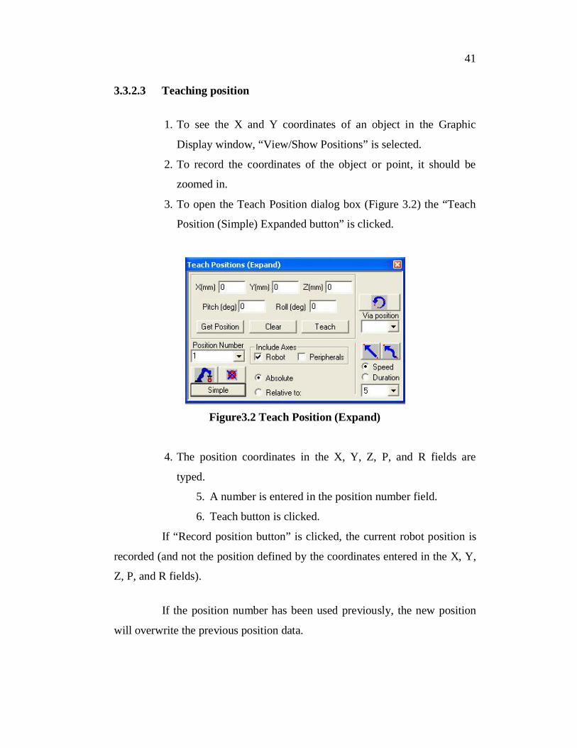
3.3.2.3 Teaching position

1. To see the X and Y coordinates of an object in the Graphic

Display window, “View/Show Positions” is selected.

2. To record the coordinates of the object or point, it should be

zoomed in.

3. To open the Teach Position dialog box (Figure 3.2) the “Teach

Position (Simple) Expanded button” is clicked.

Figure3.2 Teach Position (Expand)

4. The position coordinates in the X, Y, Z, P, and R fields are

typed.

5. A number is entered in the position number field.

6. Teach button is clicked.

If “Record position button” is clicked, the current robot position is

recorded (and not the position defined by the coordinates entered in the X, Y,

Z, P, and R fields).

If the position number has been used previously, the new position

will overwrite the previous position data.

42

3.3.2.4 Fine-tuning a position

To modify existing positions:

1. To open the Teach Position dialog box “Teach Position (Simple)

Expanded button” is clicked.

2. To modify a position, it is selected in the “Position Number

field”.

3. “Get Position” button is clicked. In the X, Y, Z, P, and R

fields,the position data appeared.

4. The required coordinate is modified.

5. To overwrite the previous position the “Teach button” is

clicked.

3.3.3 Program Execution

Executing programs in RoboCell is the same as executing programs

when using an actual robotic system. Different cell configurations can be

loaded and changed in RoboCell. But the positions and programs are not

loaded together with their workcell. For a new project, to consider workcell

and its positions, the Save as option in the File menu can be used. The project

with workcell and positions are saved under a different name. Then the

program is deleted and a new one is written. (The positions and the cell

remain unchanged).

3.4 AUTOCAD

AutoCAD is a software application for computer aided drafting. It

is a popular program because it can be customized to suit an individual's

needs. The software supports both 2D and 3D formats. The AutoCAD

software is now used in a range of industries, employed by architects, project

43

managers and engineers, amongst other professions. A few applications for

which AutoCAD is being used are as follows: Architectural drawings of all

kinds, Interior design and facility, Work–flow charts and organizational

diagrams, Proposals and presentations, Drawings for electronic, chemical,

civil, mechanical, automotive, and aerospace engineering applications,

Topographic maps and nautical charts, Yacht design, Plots and other

representations of mathematical and scientific functions, Theatre set lighting

designs, Musical scores, Technical illustrations and assembly diagrams,

Company logos, Greetings cards, Line drawings for the fine arts. In this

research it is used to validate the FKM.

One of the ways to display real-world object in a more natural way

is by adding depth to the height and width. This system uses the X Y

and Z axes. Everything that one draws in AutoCAD is exact. All objects

drawn on the screen are placed there based on a simple X,Y coordinate

system. In AutoCAD this is known as the World Coordinate System (WCS).

AutoCAD uses points to determine where an object is located. There is an

origin where it begins counting from.

AutoCAD is run in an interactive, menu–driven way and is easy to

learn and use. Because of these specific features, this software has been

selected for this research.

3.4.1 The 3D Co-ordinate System

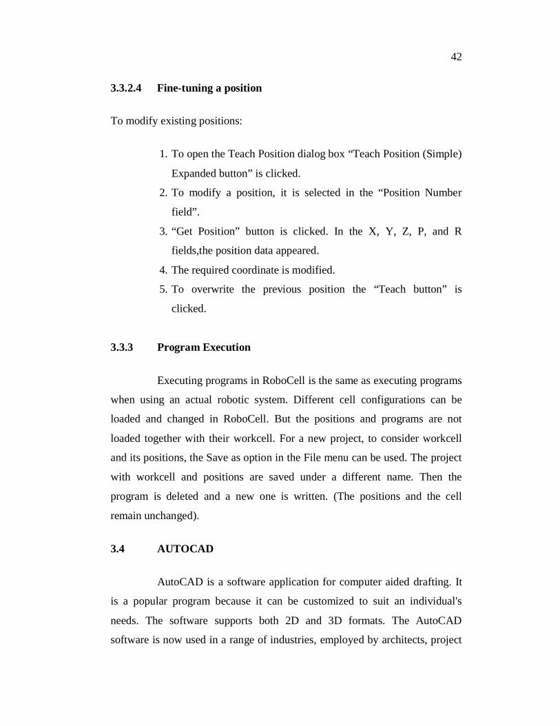
The 2D points are indicated in AutoCAD, when looking from the

plan (top) view as shown in Figure 3.3.

44

Figure 3.3 2D Co-ordinate Systems

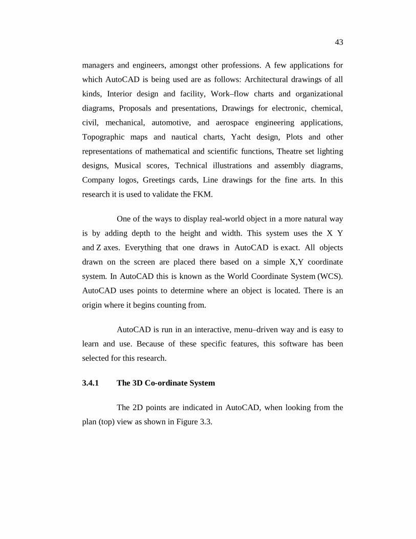
The same point is indicated in 3D spaces as shown in Figure 3.4.

The third axis is called the Z-axis. The positive Z-axis is imagined to be the

one which is coming towards the observer out of the paper.

Figure 3.4 3D Co-ordinate System

45

3.4.2 3D Visualization

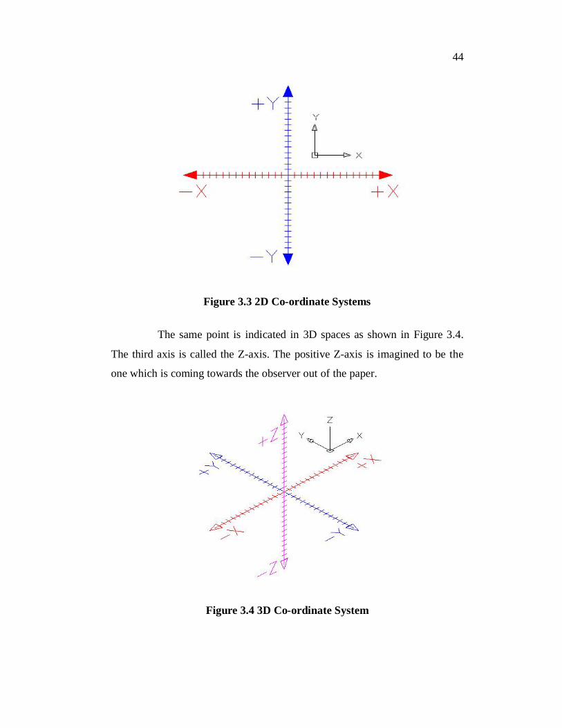
A visual style is a collection of settings that control the display of

edges and shading in the viewport. Instead of using commands and setting

system variables, the properties of the visual style are changed. Properties of a

line in 3D visualization are shown in Figure 3.5.

Figure 3.5 Properties of a line in 3D visualization

Available visual styles in drawing are: 2D wireframe, 3D hidden,

3D wireframe, conceptual, option, realistic.

3.4.3 3D Rotation

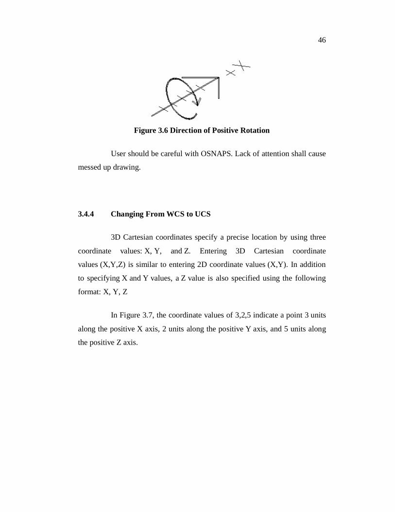
AutoCAD measures angles of rotation in 3D. There is a simple rule

for this called "The right hand rule". To figure out which is the positive

rotation angle, it is imagined that one is wrapping one’s right hand around

the axis with one’s thumb pointing towards the positive end. The direction

that one’s fingers are wrapped is the positive direction (Figure 3.6). This

applies to all three axes.

46

Figure 3.6 Direction of Positive Rotation

User should be careful with OSNAPS. Lack of attention shall cause

messed up drawing.

3.4.4 Changing From WCS to UCS

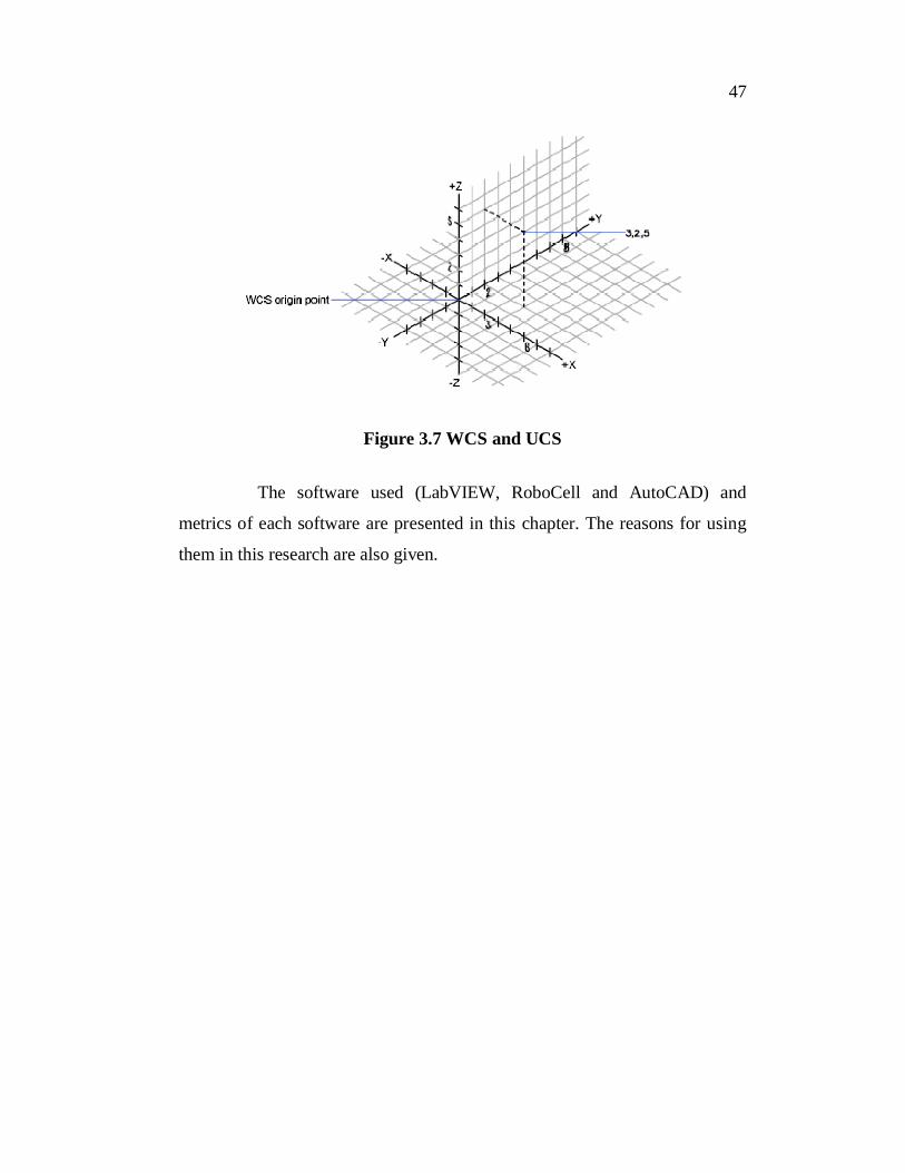
3D Cartesian coordinates specify a precise location by using three

coordinate values: X, Y, and Z. Entering 3D Cartesian coordinate

values (X,Y,Z) is similar to entering 2D coordinate values (X,Y). In addition

to specifying X and Y values, a Z value is also specified using the following

format: X, Y, Z

In Figure 3.7, the coordinate values of 3,2,5 indicate a point 3 units

along the positive X axis, 2 units along the positive Y axis, and 5 units along

the positive Z axis.

47

Figure 3.7 WCS and UCS

The software used (LabVIEW, RoboCell and AutoCAD) and

metrics of each software are presented in this chapter. The reasons for using

them in this research are also given.