CHAPTER 3 ROAD USER COSTS SURVEYS INTRODUCTION

CHAPTER 3 ROAD USER COSTS SURVEYS

INTRODUCTION

Road user costs are of primary importance in this study,

and a major portion of the total study resources will be

directed towards determining these costs. Some elements of

user costs can best be determined by experiment as discussed

in Chapter 4. However, major effort must go into surveys of

real operating costs since some factors can only be developed

from real world operating conditions.

No vehicle cost Survey of this size and complexity has

been attempted before. The nearest related study, TRRL's

Kenya Study (Ref.9), was fairly limited in extent and in the

applicability of its results. Certainly no formal methodology

has yet been established for this kind of survey and questions

about the methodology outlined here remain to be answered in

pilot studies.

Extensive resources have already been allocated to the

survey portion of the Project in terms of technical assistance

from survey experts, statisticians and economists. They

helped in devising and detailing the methodology, and we

expect to complete the task of survey design by June 1976

after analysis of pilot survey data.

Within the road users costs surveys, emphasis is also

being placed upon depreciation and vehicle maintenance costs.

These are the items about which least is presently known and

a significant effort in these areas should produce results

more valid than the judgemental values historically used.

OBJECTIVES AND SCOPE

The overall objective of the user costs surveys is to

establish relationships between various components of vehicle

operating costs and road design variables, surface roughness,

vertical and horizontal alignment, and for essentially low

volume rural roads. In order to do this it will be necessary

34

Digitised by the University of Pretoria, Library Services, 2012

to determine user costs for measurable road conditions so that

cost differentials can be determined.

The components of vehicle operating costs being consider

ed are 1) fuel 2) oil 3) tyres 4) maintenance parts 5) labour

and 6) depreciation. Maintenance and depreciation together

comprise about 50% of operating costs (see Table 3) and a major

task of the Survey is to establish sound relationships for

these components. Fuel consumption will be addressed in the

user experiments and the results calibrated using survey

data. Tyre costs comprise overall an estimated 10% of oper

ating costs, but become a major item in heavy vehicles (see

Table 2) and thus an important part of the Survey, particu

larly for buses and trucks.

In addition to the vehicle operating costs listed above

there are several other important costs. These consist of

1) crew costs, 2) interest on capital, 3) insurance, 4)

licenses and other fees, and 5) company overheads. These

costs cannot be directly related to the primary 1ndependent

variables of surface type, roughness, and geometry. Although

cost items, they will receive only minor attention during the

Survey.

Initially the Survey will be conducted in the states of

Goias and Minas Gerais and the Federal District of Brasilia.

These areas should satisfy Survey needs in terms of extremes

of roughness and geometry. Studies in other states may be

required to determine the effects of traffic congestion on

gravel roads or to obtain a wider range of depreciation data.

Therefore additional satellite studies will be undertaken

later to fill any gaps in the Survey as required.

During preliminary evaluations it was established that

the cost of data collection must be a primary input to the

survey design. Thus an evaluation must be made of the import

ance, or priority, of all data items, to centro: costs and

maximize benefits. An evaluation of data collection costs

will be made during the pilot study (March-June 1976) and by

June a fairly objective estimate of the scope of the Survey

in terms of numbers of vehicles will be available.

35


w

""

TABLE 3 IMPACT OF COSTS BY COST ELEMENT AND VEHICLE CLASS, INCLUDING TAXES, ON THE VEHICLE POPULATION OF MINAS GERAIS AND GOIAS, EXCLUDING VEHICLES IN THE URBAN AREAS OF BELO HORIZONTE AND GOIANIA. ANNUAL COSTS IN MILLIONS OF CRUZEIROS, DECEMBER 1975

VEHICLE CLASS FUEL OIL TYRES MAINTENANCE DEPRECIATION TOTAL

CAR 726 58 57 265 468 1574

UTILITY 1045 73 79 564 653 2414

BUS 176 37 69 184 180 646

TRUCK 1040 219 756 1089 792 3896

TOTAL 2987 387 961 2102 2093 8530

PERCENTAGE 35.0 4.5 11.3 24.6 24.5 100

-----------

Source- 16,17,18

Note: Figures are rounded.


w .......)

TABLE 4 AVERAGE OPERATING COSTS FOR TYPICAL VEHICLES IN FOUR MAIN CLASSES, BY COST ELEMENT. COSTS IN CRUZEIROS PER KILOMETRE INCLUDING TAXES AT DECEMBER 1975

VEHICLE CLASS FUEL OIL TYRES MAINTENANCE DEPRECIATION TOTAL Cr$ PER KM

CAR (4 pass.) .3102 .0250 .0242 .1135 .2000 0.6729

Vtv 1300 Sedan 46 4 3.5 17 29.5 100%

UTILITY (LIGHT) .4653 • 0324 . 0350 .2510 .2905 1.0742

Chevrolet C 10 43 3 4 23 27 100%

BUS ( 36 pass.) . 4 762 .1004 .1850 . 4985 • 4861 1.7462

Mercedes 0-362 27 6 10.5 28.5 28 100%

TRUCK - 3 axle .4762 .1004 • 3462 .4985 .3625 1.7838

Mercedes 1113 27 5.5 19.5 28 20 100% -- ------~·· - -- -- -

Sources 17,18


MAJOR COSTS ELEMENTS

Before describing the Survey design being considered for

use in the Project it is appropriate to discuss the various

elements of vehicle operating costs and examine their impact

from information already available. This is done below with

particular attention to Brazil.

Vehicle Depreciation

It seems logical to assume that vehicles which are driven

primarily on rough, unpaved roads will wear out, physically

deteriorate, and therefore depreciate in value more rapidly

than those vehicles used primarily on smooth, paved roads.

Many logical assumptions are wrong, however. If prospective

buyers had perfect information about the vehicles they were

considering for purchase, they might indeed be less willing

to buy vehicles which had been driven on rough roads, thus

forcing a lowering of their prices.

If prospective buyers do not know the history of the

vehicles they consider for purchase, having been driven on

rough roads may not affect the price of these vehicles at all.

It is an empirical question. Since we are working in a market

economy and in general accepting the price (market value) of

each commodity as its value, it would be inconsistent to try

to find some "real" or intrinsic depreciation of these vehi

cles. We must accept their market value as their true value,

and the reduction in market value as the depreciation.

Thus there are two steps in the process of measuring

depreciation. 1) Obtain a measure of depreciation for each

class of vehicle. 2) Obtain a measure of the difference in

resale value attributable to each vehicle class having been

used under different highway conditions.

For the first item Table 5 shows calculations based on

industry data for used vehicle sales in Rio and Sao Paulo as

of September, 1975. More data sources are being sought and

similar calculations will be made. In most countries, auto

mobiles seem to lose a fixed percentage of their current value

each year. In Brazil, inflation complicates these calcula -

38


TABLE 5 PERCENT OF 1975 MODEL VALUE~~INTAINED BY EARLIER YEAR MODELS, FOR BRAZILIAN AUTOS

1975 1974 1973 1972 1971 1970 1969

FORD --Cor eel 100 85.2 75.0 63.2 54.4 46.3 39.2 Belina 100 85.4 74.4 64.5 55.6 47.1 -Maverick 100 86.4 72.4 - - - -Galaxie 500 100 79.0 65.3 47.2 37.9 30.3 25.0 Rural 100 82.5 68.5 59.1 51.6 45.9 38.2 Jeep 100 86.0 75.0 6 3. 8 55.0 47.4 42.0

CHRYSLER

Dodge Dart 100 81.8 68.3 54.0 43.7 36.7 30.2 Dodge CI:arger 100 76.9 64.8 49.7 40.7 - -

G.M.

Opal a 4 cyl. 100 83.7 70.8 58.9 50.6 43.1 36.5 lop ala 6 cyl. 100 78.2 57.4 54.8 57.4 39.5 33.4 IVeraneio 100 81.7 6 7. 0 57.0 48.8 41.1 35.2

PUMA

Puma GTE 100 81.2 71.2 62.6 53.8 48.3 41.8

v.w.

Brasilia 100 89.3 81.1 - - - -Kombi 100 87.1 77.0 65.3 57.3 50.9 43.7 rvw 1300 100 89.9 79.9 70.6 62.0 55.9 50.3 vw 1500 100 86.2 74.4 65.3 57.4 50.9 -Average Percentage 100 83.8 71.4 59.9 51.9 44.9 37.8

15% Deprecia-tion 100 85.0 72.3 61.4 52.2 44.4 37.7

Data from Quatro Rodas ''Automobile Harket" report based on sales prices in S~o Paulo and Rio de Janeiro. October 1975.

39

1968

---

20.5

33.6

38.8

--

--

31.6

35.5

-38.5

44.4

-

34.7

32.1


tions, but for automobile models which have been produced for

several years without major design changes, the prices as of

September 1975 have been used to calculate the price on that

date of each preceding model year as a percentage of the 1975

price. The data seem to indicate that autos have a resale

value approximately given by the formula

RV = B (0.85)n

where RV = resale value B = the base price of the 1975 model in

September 1975 n = age of auto in September 1975, in

years, given by: n = (1975 - model year)

Similar data and calculations are needed for trucks and

buses.

The second step in the analysis of depreciation will

involve obtaining information from dealers as to the differ

ence in resale value of vehicles which have been driven large

ly on smooth, paved roads. This may be done through the

Delphi process of getting groups of dealers together and seek

ing a consensus estimate, or it may be done by administering

questionnaires to dealers.

It is proposed to attempt the Delphi method, making

preliminary investigations amongst dealers in Brasilia, before

organization of a wide-spread survey, covering several areas

of Brazil. Information on depreciation will be sought from

the vehicles in the main survey, but it is considered likely,

as in the Kenya study, that relying on these alone for our

sample will yield insufficient data.

Vehicle Maintenance

Vehicle maintenance (parts and labour) is a major compo-·

nent of operating costs for all vehicles (see Table 4}. It

is necessary to separate the elements of parts and labour

since the relative unit costs of these items varies from time

to time and more importantly, from region to region. The

40


ratio of part costs to labour costs also varies for different

maintenance operations. This is illustrated in Table 6 for a

city bus fleet in Bradford, England.

Maintenance consumption, unlike fuel, oil, and tyres,

does not vary uniformly with distance travelled, and this

makes measurement more difficult. The numerous different

parts must wear out or fail in service and be replaced before

consumption can be measured. Thus for study purposes a long

period of time is required to measure true consumption rates.

These rates vary considerably over the life of the vehicle

since different items require replacement or attention at

different time or accumulated travel intervals.

Possible relationships between highway characteristics

and vehicle maintenance costs follow.

Vertical Geometry - the number and steepness of grades

contributes to engine, clutch, gearbox and differential wear.

Wear is greatest on up or plus grades but is al~o affected on

down or minus grades. In addition, minus grades affect brake

wear.

Horizontal Curvature - affects engine and gearbox wear

through required speed changes. Steering gear, springs and

shock absorbers are affected by sideways forces.

Surface Type and Roughness - affects every part of the

vehicle in some degree, but particularly steering and suspen

sion, electrical parts, chassis and body.

Other related factors contributing to overall mainte -

nance costs during the life of the vehicles are a)driver

behaviour, b) vehicle use, and c) owner's maintenance policies.

a) driver behaviour - may affect maintenance cost per

km much as it does fuel consumption. Excessive

speed and acceleration contribute to engine wear,

hard braking to brake wear;

b) vehicle use - conditions of use affect maintenance

costs. Traffic congestion, frequent loading and

unloading for commercial vehicles, causing engine

and brake wear, and bodywork damage, respectively.

41


TABLE 6

Item

Painting

Bodywork

Electrical

Chassis and

Engine

Transmission

MAINTENANCE AND REPAIRS - LABOUR COpT AS A PERCENT OF TOTAL COSTS FOR A FLEET OF BUSES IN BRADFORD, UK

Labour as a Percent of Total

94

83

71

Brakes 67

60

27

Source - R. Travers Morgan and Partners, London "Costing of Bus Operations" Interim Report July 1974.

42


c) maintenance policy - poor maintenance and irregular

servicing causes premature failure of parts, and

shortens the vehicle's effective life, thus adding

to depreciation cost as well as to parts consumption.

Vehicle "downtime" is an important consideration for

commercial vehicle operators, and it is often

difficult to select an optimal maintenance policy.

Decisions required include 1) when to remove the

vehicle from operation for inspection and preventive

maintenance, 2) how frequent should servicing

intervals be to avoid costly breakdowns, and 3)

should new or reconditioned spare parts. be used

etc. Operators usually arrive at such decisions by

trial and error and such policies vary to suit their

own opinions and peculiar circumstances.

Fuel Consumption

Fuel is a major cost element in all vehicle classes,

and remains so whether considering commercial prices or

economic or shadow prices. It is particularly important for

cars and other gasoline vehicles when considering the

commercial price, since this class (mainly private vehicles),

often subsidizes diesel vehicles (mainly commercial vehicles)

through a higher rate of fuel tax.

From a survey point of view, fuel consumption has the

following characteristics:

Tyres

1) varies directly with distance travelled 2) is the simplest cost item to measure 3) variation in consumption rates reveal themselves

quickly 4) can be used to calibrate experimental data 5) most operators keep records 6) can be used to check data on other costs items (in

fuel consumption data is suspect, so is other data)

Highway surface characteristics have a direct and

obvious effect on tyre wear since the vehicles tyres are in

direct contact with the road. Surface roughness on both

paved and unpaved roads is therefore a major factor in tyre

wear. However vertical and horizontal geometry are also

43


known to have effects on tyre wear, in association with

vehicle speed and direction changes causing abrasion or

sloppage. Another factor, particularly important for heavy

vehicles, is weight carried per axle.

Oil Consumption

Oil consumption is a relatively minor item of operating

cost in all vehicles, usually representing less than 2% of

total operating costs. It is probable that engine and gearbox

oil consumption is much more directly related to engine wear

than conditions of vehicles use.

Other Costs

a) Crew Costs - This information may be derived from

operators, organizations such as National Highway

Freight Transportation Association (NTC) , and

official sources. In general, crew costs increase

with the size of the vehicle, particularly for

freight vehicles but also to some extent for buses.

b) Interest on Capital - In most estimates of vehicle

operating costs, an interest or finance charge is

included, often lumped together, or hidden within,

depreciation costs. In the present study it is

hoped to derive reliable estimates for vehicle

depreciation and capital on interest charges in

each year of vehicle .life, and a set of age spectra

for each vehicle class.

c) Insurance - In most countries some form of insur

ance coverage is compulsory and is included as a

component of vehicle operating cost. Tariffs

issued by insurance companies and amounts paid by

vehicle operators usually reflect the claims

experience in the preceding year or few years.

d) Licences and Other Fees - Annual vehicle licences

for each vehicle class can be calculated easily

by reference to TRU (Taxa Rodoviaria Onica) tables

for any year.

44


e) Company Overheads - This item covers all other

essential items of expenditure connected with vehicle

operations not already listed above. Overheads

typically include rental costs for offices and work

shops, clerical and management salaries, insurance

(other than vehicle insurance), accountancy fees,

power light and heat, telephones, stationery and

postage, and may include other items, such as

advertising.

SURVEY DESIGN AND METHODOLOGY

Many questions remain to be answered regarding sample

design and survey methodology. This section summarizes the

current state of the problem and accomplishments. An inten

sive study of the survey approach and its strengths and

limitations is currently underway as outlined with our

sponsors and the Expert Working Group (EWG) in December.

Preliminary proposals for the survey design for buses,

trucks, utility vehicles and cars are also presented in this

section. These proposals will be refined and revised in the

next three months through the inputs of the experts mentioned

later and the survey group.

To effectively design a survey a wide variety of informa

tion is required, as follows:

1) the exact objectives of the survey stated in terms of

data inputs

2) data on the vehicle population

3) data on route characteristics used by the vehicle

population

4) knowledge of problems likely to be encountered during

data collection.

At the present time three major activities are underway

to gain this required information. These three activities

will assist in developing an effective final survey design

for use in the road user costs surveys.

45


1) Gathering background information in pre-pilot studies

2) Consultation with survey design experts

3) Testing survey instruments in "pilot studies."

Background Data Collection Techniques and Sources

In the initial interviews, many items of information will

be recorded. Field personnel will first assess the

operator's willingness to cooperate and secondly, his ability

to do so. The following types of information will be

investigated in pilot studies.

Does he keep records?

What items are recorded and how?

What items are missing?

Is information compiled separately for each vehicle?

Are routes and vehicle arrival and departure times noted?

Are tachographs used?

Are loads and passengers recorded for each trip?

Are all invoices, vouchers and receipts kept to support

cost control summaries?

Will the field team have access to all supporting

documents?

What checks does the operator himself carry out to

ensure accurate records?

If formal records are incomplete, can they be compiled

from invoices and other documents?

Can the team assist the operator to establish a reliable

information system?

Where formal records are not kept, the operator will be

encouraged to begin doing so and the team will assist him in

setting up a cost control system, monitored by senior project

personnel. Original evidence, particularly invoices, will

then be checked wherever possible, rather than relying on the

summary totals produced by the operator himself. Where

records are kept by the operator, data will normally be taken

directly from them, but only after checking the recording

system for accuracy and reliability.

46


Data collection will consist primarily of repeated visits

with the operators of sample vehicles. Project personnel will

visit each operator at least once per month to complete a set

of forms designed to obtain all the information shown in Table

7 for "Interviews- Vehicle Operator's Records."

Often during the regular data collection phase the opera

tor's goodwill will be tested to the utmost by requests for

"this document," nthat ledger," "those invoices,n etc. Tact

and patience will be required from the field team to avoid

pushing too far on the one hand and to recognize on the other,

the appropriate moments to make requests.

In survey terminology the field personnel must be extreme

ly skilled at building and maintaining "rapport" with the

operators, since the nature of the data sought, as well as the

number of visits required for collection, will require such

skills.

In addition to the vehicle operators, information will be

sought from a variety of other sources. These include vehicle

and tyre distributors, repair shops, NTC (National Highway

Freight Transportation Association - Associagao Nacional de Em

presas de Transporte Rodoviario de Carga), DNER and DER's.

Physical measurements of roughness, and vertical and

horizontal geometry, are extremely important to the road user

costs surveys and are covered in detail in Chapter 6.

Table 7 summarizes the variables for which data will be

collected and identifies for each the sources which the

research team will access to obtain the data.

Consultation - Survey Design Experts

Several experts have been contacted to assist the survey

team in the design and development of the survey. Presently,

Mr. Paul Moore, formerly of Research Triangle Institute (RTI)

and now a sampling statistician for USAID with Institute Bra

sileiro de Geografia e Estatistica (IBGE) in Rio de Janeiro,

is contributing time and giving useful ideas under an informal

exchange agreements with TRDF.

In late December 1975, Messrs. Wyatt, Odilon, Hudson and

47


~ 00

TABLE 7 DATA COLLECTION ITEMS AND SOURCES

Interviews - Vehicle Operator's Records

Physical Measurements Mays Meter Inclinometer Traffic Counters Maps

Independent Variables

1. Age of Vehicle 2. Payloads, Freight and

Passengers 3. Distance Travelled 4. Time Spent on Route 5. Number of Stops on Route

and Time Loading and Unloading

6. Traffic Delays and Congestion

7. Vehicle Speed

1. Traffic Volume and Composition

2. Road Surface Type 3. Roughness 4. Vertical Geometry

Meters of Rise and Fall by Surface Type

5. Horizontal Geometry Degrees of Curvature by Surface Type

Dependent Variables

Consumption & Cost of -

1. Fuel 2. Oil and Greese

3. Tyres 4. Maintenance Parts 5. Maintenance Labour

6. Accident Costs

7. Crew Time

Other information

1. Fleet Size 2. Nature of Business

3. Bus Tariffs 4. Haulage Rates 5. Vehicle Specifica

tions

6. Other backgroung, · e. g. growth, 7. Labour Hourly

Rates

(Continued)


~ 1..0

TABLE 7 (Continued)

~ e

Other Sources -DNER DER' s Vehicle Distributors Repair Shops Tyre Distributors IPR NTC

'---------

Independent Variables

1. Traffic Volume and Composition

2. Bus Passenger Counts

Dependent Variables Other Information

1. Depreciation from 1. Blading frequencies Interviews and Delphi for unpaved routes Surveys

2. Parts and Labour Costs 2. Taxes and Duties on Fuel, Tyres, Spare Parts.


Moser, of the project staff, and Professor Anderson, consult

ant, spent four days discussing with Mr. Moore possible

approaches for the survey. Other meeting and telephone

conversations have taken place since that time and additional

working sessions are planned.

In addition, Dr. Wade Clifton joined the staff in early

February and has begun a study of the problems. Dr. Clifton,

a survey research economist from University of Texas, will

remain to assist the staff here until mid-April and can be

available subsequently. Prior to that time, Professors A. A.

Walters and Cheshire, consultants to the World Bank and Dr.

Rob Harrison of the University of Aston in Birmingham, England,

will arrive for discussions in late March 1976 to assist with

finalizing the survey designs.

Pre-Pilot Studies

In order to obtain necessary information for planning the

Surveys, pre-pilot and pilot study activities were planned in

December 1975. A list of the tasks for these studies is given

below. These are followed by the preliminary survey designs

for buses, trucks, utility vehicles, and cars.

Pre-Pilot Study Tasks October 1975 - February 1976

1) Interview fleet owners, NTC, vehicle distributors and

"autonomos" unions to obtain background informa-

tion on a) vehicle types,· b) operating costs, c) the

structure of the bus and freight industry, and d)

trends in the industry;

2) Contact otherslikely to have an interest in the sur

vey: IBGE and Institute de Pesquisas Rodoviarias(IPR);

3) Obtain vehicle population data from various agencies

including DNER, DER-GO, SUTEG, DER-MG, DER-DF, SERPRO

headquarters and regional offices, and NTC;

4) Visit DNER, DER-GO, DER-MG and DER-DF for information

on characteristics of selected routes;

5) Appraise the data collection problems likely to be

encountered from further interviews with vehicle

owners;

50


6) Design and pre-test the data collection documents.

Tasks 1-5 have been completed except for item 3 where

negotiations are currently in progress with SERPRO to supply

TRU records of vehicle population, fleet sizes and addresses

of owners in Minas Gerais, Goias and the Federal District.

Task 6, the initial design of the documents has been completed

(see Figures 7, 8, and 9) and pre-testing will commence on 9th

March in a short data _collection exercise.

Pilot Studies

The primary objective of the pilot studies as outlined

below is to test the practicality of the survey designs for

efficient selection of vehicles whose routes have the required

discrimination in the independent variables 1) surface type,

2) roughness, 3) vertical geometry and 4) horizontal geometry.

The number of companies and vehicles selected for actual data

collection will be small, probably four or five companies, one

or two "autonomos", and a total of 30 or 40 vehicles. Because

of the short time span, 3 months, the data collected is

unlikely to yield positive results for prediction equations.

However the data collected will be sufficient to fulfill the

second major objective, to provide the team with experience

in data collection, coding and analysis, and evaluation of

data collection costs, as an input to the main survey design.

Pilot Study Tasks March-June 1976

1) Assemble vehicle population data for buses, trucks,

utility vehicles and cars and array with corresponding

available data on route characteristics;

2) Select pilot-study participant companies in a first

stage sample (see below under section "Preliminary

Survey Designs");

3) Obtain more detailed information on road characteris

tics for the companies' routes;

4) Select a second-stage sample of participants and

check routes with the Maysmeter;

51


ROTA USADA l l I I I l l I I I I l I I I

CONSUMO DE COMBUSTIVEL

CON SUMO VELOCiMETRO

CON SUMO VELOCfMETRO DIA DIA

LTS CrS LTS Cr $

-+-+-i-t-+· .. L ···J 11 l l J I I . ····[·-+-·+··+··-- L ___ __ Lt-{---- I I 1 l

I l I I ·-·1 I I I I l l l l l I I l I I l l

l l l 1 I l l I I I I l I I I I l I I I l I l l l I I I I I I 1 l

l I I I l l I J J I I I I I I l I l I I I I I I I l I I l l I I I I I I I I l I I l l l I l I I I I I I I I I I l ! u l l I I I I I I I I l Li I I l l l l l I I I I I I I I I I I I I I I I I I I I I j __ .l __ u__j_J _ _L I I I I I I I I I

! I I I I I I I I I I I I I I I I I I I I I J_j_U_j l l I I l I I I I I

I l_ I I I I I I I I I I I I I I I I I J±-li- I I I I I I I I l l I

_L.__Lj_J__ Ll_ l J l l I _I I I I J TOTAlS I I I I I

6LEO DO MOTOR

VELOciMETRO DIA ~~~SUMO Cr $ VELOC(METRO DIA ~~~SUMO Cr S

I I I l I I . L I I I 1. .. -f-1-~ll__..L._ i1 _.~__l-t-~1-LI---.Jl:---1-'-----t-~1-!-1~ 11~1--1

l l Ll_L_ I I I l _L _ ___Ll_lL__l_l ~~~__J____JI_J-'-----t----":-1_..___,_11 ---7-1~1~ I 1 J l J _j __ j__J_j_L+--LI ___l_!----L-1 _.L_J -t-~I__J_____JIL_J-'-+___J.II _ _.___._

11

1

1 _._1I_J'----1

1 I I _ I I I I _U_j__l_-+-..J...___L_J ___LJ__JlL--+--_.~__1 -+--!___L_II __~_l-+--~~-'---1 I I I l l 1 _ Ll_l. _ _LI ___Ll-+-J_I __~_I ___j_I_IL___f---'--1-+-L__L_I __._J -+-~11 _,__I__._I_L'--1 I I J j __ r-__l___l_L_B_ I I I I I I l : : l : : : : l I I I I _l_L_L __j___l_j___j___l------l-' -_l_l ___~l_lL___.f--~f-------L-~~--'-1 ___.~-~ 11_._1--1

U-1-j_J_J - __ L ~ .. Lj_J_ __ j __ j_l_j __ j I J 1.---'J~T..L.OT--'-A~S-t----7-1 --_Jl'---1~-~11----!-1-~ IJ ---1

GRAXAS OUTROS OLEOS

VELOdMETRO DIA CONSUMO A?REV VELOdMETRO DIA CONSUMO KG Cr$ OLEO LTS CrS

l l l l 1 l _ll I I I I I I l l I l l 1 I I l 1 l I I I l J_ ~j_l_j_ _ __Lllll__ _ __ .J...___l__ II --'-1 ___L_l -f--LI---1-l.L-1.-1 _.__l -+---'--: __._~ ___..}~f-j"'---1

t-----'---'J~J_LL _L __ l ___ J_l ___ LJ_llJ_r----- __ j_J.L.._j_J ___LJ-+--..L..._f-l~j-{L_j~~1 -1.__~11 ~1--; I I I l __ r--_1-~Ul_U_LLJ j_ -- _L_l _ __JIL__~I---LI---f--.l...-....l.-11 --'-1-t--'--1-'----'--II -'-1--'l----j t----'----'-1_..__! _l_l_ __L _ r-ll_l ___ U_L_L __ j__ I~ 1-+___LI_JL_J..L_LJ -f--J-

11--+-

1J__.L_

1 ---Ll-t-~1 ~ I' ---7-l-:-l-;

TOTAlS l ! I I I I I I I I I I l OBSERVACOES

____ LL __ L...L_I -+---'-:--+-_,__1 __._l __,_1-t--[.___.__._lt _._f ~f--~ r---- _l__Lj__j__J -t-~-LI __jl_~ 1 -'-1-IL_-'----'--11-'-1-; r- I I I I I I I I

TOTAlS I I I I I I I I

Figure 7 Data Collection Document for Fuel, Oil and Grease. Note·Actual Size is 18 x 28 em.

52


CONTROLE DE PNEUS

NOME DA EMPRESA: Mb: ANO: __

VE(CULO N2: PLACA: MARCA:

TIPO DO VE(CULO: MODELO: ANO FABRICACAO:

ROTA USAOA:

EST ADO INSTALACAO RETIRAOA

NUMERO DO PNEU VELOCiMETRO DATA VELOCiMETRO DATA OBSERVACOES

I I I I I I I I I I I I I I I I I I I I I I I I I

I I I I I I I I I I I I I I I I I I I 1 I I I I I I I I I I I I I I I I I I I I I I I I I I I I I I

I I I I I I I I I I I 1 I _l I I I I I I I I I I I

I I I I I I I I l I I I I I I I I I I I I I I I I



I I I I I I I I I I I I I I I I I I I I I I I I I I I I I I I I I I I I I I I I I I I I I I I I I I



I I I I I I I 11 I I I I I I I I I I I I I I I I I I I I I I I I I I I I I I I I I I I I I I I I I

I I I I I r I I I I I I I I I I I t J J 1 I I I I







I I I I I I I I I I I I I I I I I I I I I I I J I





.I I I I I I I I I I I I I I I I I I I I I I I I I CODIGOS:

ESTADO DO PNEU OBSERVACOES

NOVO PARA OUTRO VE(CULO

Figure 8

RECAPAOO PARA RECA PAGE M

INUTILIZAOO

Data Collection nocument for Tyres Note. Actual size is 21 em x 26 ern.

53


U1 ~

CONTROLE DE SERVICO DE OFICINA

NOME DA EMPRESA I I I I I I I I I I I I I I I I I I I I I i I I I I I I I I I I I I I I M~S Ll_j ANO Ll_j VEiCULO NUMERO I I I I I I I I I I I I I I I I MARCA I I I I I I I I I I I I I I I I I PLACA l I I I 1 .I I I I I I TIPO DO VEI'CULO I I I I I I I I I I I I I I I I MODELOI I I I I I I I I I I I I I I I I ANO FABRICACAO I I

I I I I I I I I I I I I I I I I I I I I I I I I I I I I I 1 I CdOIGO ROTA USADA

I I I I I 1 I I I I I I I L J l I I I I L I I I I I I I L J VELOCfMETRO

CAUSA CODIGO REFER~NCIA MAO DE OBRA

DIA DO SERVICO N2 HORAS CrS

VALOR PECAS CUSTO TOTAL SEIM(X

I I I I I I I I I I I I I I I L I I I I I I I I I I I I I I I I I I I I I I I I I I I I I I I I I I I I I I I I I I I I I I I I I I I I I I I I I J I l I I I I I I l I I I 1 I I l I I I 1 l_ I I I I I I I I l I I I l I I I I I I I I I I I I I I I I I I I I I _I I I I I I I I I I I I I I

_Lj_j_____l 1 I I I I I I I I I I J I I I I I I J I L I L J l I l I I I I I I I I I I I I I I I I I I I I I . I I I I I I I I I I I I I I I I I I I I I I I I I I I I I I I I I I I I I I I I I I I I I I I I I I I I I I I I I I I l 1 I I I l I I I I L I I I I I I I I I I I I I l l I I I I I I I IJ I I I I I I I I

u_u___LJ_ I I I I I I I I I I I I I I I I I I I I I I I I I I I I I I I I I I I I I I I I I I I l l I I I I I I I I I L l I I I I I I I I l l I I I I I I I I l I I I 1 I I IIIII U Ill I I I I I I I I I I I I I I I j__J_J_ I I I I I I l I I I I l I l l 1 J J l l _l__j__j_ _ _ u__j_ _ _l_j_ _ _LLLLL__LU I I I I I L I I I I I I I I I I I I ILLLLU __ r--j____ I I I I I I I I _l___l~ I I I I I I I I l l 1 l I I l I I I I I I L I I I I J _L _ _LL I I I .1 I I I I I I I I I I I l I I I l I I I I I I l I l I I 1 l l I I l l l J l I l I I I I I I I I I I I _l_l I I _L_LL__L j ___ L_Ll__L_L_LJ _ __L __ _ l I I J I l I I I I I I I I I I I I I I I I I I I I I I j__J_J___Ll_l_L__L _j I I I I I I I I I I I I I I I I I I I I I I I I I I I I I I_U I I I __L_LLL_LLL_l__j _l __ __ j __ L l _ I I I I I I l I I I I I l __l I I I I I I I I I l - I I I I __ _ Ll_j_J __ LJ_~_j ___ j_ I I I _ L __ L_ __ _L__j_ _ _L I I I I I I I I I I L I I I

u_j_J__Ll I _ l___ __ j__j_ ___ ]___ _ _ _L ___ L __ L_l~_LL_Lj___ _Ll_ __ l __ _l_j _j_ _ __ _j_ ____ L_L_L I I I l_ I I I I j_j_ I I I I I I I I I I I l__l___L_ _ _u___ .. L J _Ll__Ll_ _ _L_L__l__ I -· I I _c_j_ __ _l____j__ _1_. U-J_J _ I I I I I I I I I I I I I I I I I I I I I I I I I I I I I I I I I I I I I I I I I I I I I I I I I I I I I I I I I I J 1

TOTAlS I I l I I I I I I I I I I I I I I I I I I OBSERVAC0ES

-----

Figure 9 Data Collection Document for Maintenance Parts and Labour. Note. Actual Size is 17 x 29 em.


5) Conduct initial interviews on routes, vehicles and

records available;

6) Arrange programme of visits and commence data collec-

tion;

7) Code data inputs;

8) Develop specifications for output programmes;

9) Analyze data;

10) Conduct progress checks and monitor data collection

costs;

11) Develop pilot study report including final proposals

on survey design.

PRELIMINARY SURVEY DESIGNS

The States of Goias and Minas Gerais together have a

population of approximately 3,455 intercity buses, owned by

375 companies and operating on 1,300 lines, totalling about

100,000 kilometers in route length (Ref. DER-GO and DER-MG).

The distribution of bus company fleet sizes is shown in

Figures 10 and 11. In addition, there are approximately

2,500 buses operating on urban routes which will not be

considered for purposes of this study. In these two states

there are also 258,000 cars, 98,100 utility vehicles, and

48,500 trucks (Ref. 16).

Given vehicle populations of these sizes, which for all

classes represent about 10% of the Brazilian total, we hope

to be able to locate sufficient numbers of vehicles operating

on extreme route conditions.

Preliminary Survey Design - Buses

There is a probability that if a company has a large

number of routes then for operational reasons the buses will

change routes quite frequently. In general, the larger the

number of routes and buses, the greater the likelihood of

frequent route changes for any vehicle. This mixing of the

effects of route characteristics will make it difficult to

find vehicles operating consistently under extreme route

conditions of roughness or geometry during the 30-month data

collection period. Therefore companies will be stratified on

55


programme of roughness measurements. Additional companies will

be selected if the initial sample routes do not adequately

cover the expected range of roughness.

A final selection of buses will be made by contacting

the companies to request their cooperation in data collection.

An initial questionnaire will be completed to check route data,

and compile details of each fleet, checking vehicle age

spectra. Companies will be oversampled to allow for non

cooperation, or inadequate cost records, and vehicles over

sampled to allow for accidents and vehicle disposals.

Preliminary Survey Design - Trucks, Utility Vehicles, and Cars

Unlike buses, where much useful information has been made

available from the records of DNER and other agencies, far

less initial information is available for trucks, utility

vehicles and cars. While most buses, or bus companies, have

defined routes, the majority of trucks, utilitiea, and cars,

do not. Furthermore, no published information is available on

those who may operate regular trips on defined routes. Thus

the task of finding vehicles traversing mostly routes of a

homogeneous nature becomes difficult.

Geographic stratification will be used to classify road

usage as mostly paved, unpaved or mixed. Centers of popula

tion will be classified by size, and grouped in a number of

geographic areas according to distance from the main paved

road networks. Large population centers are normally closer

to paved roads. However a number of towns in northern Minas

Gerais have already been noted which are up to 200 km from

the nearest paved roads. Four centres of between 5 and 10

thousand people and one between 10 and 50 thousand have been

identified.

Estimates based on vehicle ownership (see Table 8) indi

cate perhaps 500 cars, 250 utilities, 40 buses and 130 trucks

as the vehicle universe in this "mostly unpaved" region.

A register of the vehicle universe, at least for the

main study area, is considered essential and is being

obtained through DNER, from TRU records held by SERPRO on

magnetic tapes. From the TRU records, owners names and

56


TABLE 8 VEHICLE OWNERSHIP

VEHICLE PER 1,000 OF POPULATION

GOIAS MINAS FEDERAL BRASIL KENYA GERAIS DIS'IRICI'

CARS 12.9 17.0 73.0 31.0 6.4

UTILITIES 5.4 6.4 13.4 8.4 4.1

BUSES 0.25 0.45 1.5 0.55 0.30

TRUCKS 2.1 3.3 3.9 4.8 1.6

Notes:

1) Vehicle figures TRU 1974. Population figures for Brazil from the 1970 census plus 10%.

2) Kenya population estimated as 10 million. Vehicles figures for 1973 from TRRL Report 672.

3) Cars - Compare:

Western Europe - 1970, 228 per 1000 U.S.A. - 1970, 434 per 1000

57


lJ1 00

16

15 -0 14 ,._ 0 ._

13 '+-0 12 Q) 0 II 0 ~

10 c Q) 0 9 L.. Cl> a. 8

I -o c 7 0

~ 6 0 c Q) 5 ::J 0"

4 Q) L..

lL. 3 I

U) 2 Q) (/)

::J CD

0 2 3 4 5 6 7-10 11-15 16-20

Fleet Size

Figure 10 - Percentage and Frequency Distribution of Bus and Fleet Size for Intermuniqipal Companies in the States of Goias and Minas Gerais.



the basis of whether their routes in general are "mostly

paved", "mixed", or "mostly unpaved". The total length of

each route will be divided into paved and unpaved. These

totals will be summed for all routes and the total route

length of each company expressed as total kilometers and

percentage unpaved. Paved and unpaved sections of each route

will be multiplied by trip frequency (number of buses per

week) and the totals of paved and unpaved for all routes sum

med again. The total vehicle distance travelled will be

expressed as total kilometers and percentage unpaved. This

may be a more useful figure than total route length since it

characterizes the average amounts of paved and unpaved travel

for any vehicle. We can now stratify each company into

"mostly paved,""mixed" and "mostly unpaved" on the basis of

vehicle distance travelled.

The companies will be stratified based on operating

locations into geographic regions characterized~as mostly

hilly or mostly flat, so that the first stage of sampling will

have a better chance of including hilly and flat routes. The

proposed strata are shown in Figure 12.

From each stratum a sample of companies will be chosen,

taking medium or larger companies where possible. This will

be done to obtain as many buses as possible on different route

types and to reduce the number of companies to be visited

during the pilot survey. A higher proportion of companies

will be selected from the "mostly paved" and "mostly unpaved"

strata since they represent the extreme characteristics of

the routes.

The actual hilliness of the routes of each company chosen

will be investigated in detail, from road profiles where

available or from the 40-metre interval contour maps. The

sample companies will then be stratified on the basis of

"steep," "medium" or "flat" routes. At this stage a check will

be made to ensure that an adequate range of vertical geometry

has been obtained. The strata are illustrated in Figure 13.

An initial sample of unpaved routes will be measured in diffe;

ent geographic areas using the Maysmeter, prior to the full

60


Mostly Paved Middle Mostly Unpaved

Companies N9 of Companies N9 of Companies N9 of Buses Buses Buses

-4-J ro

r-1 r:r..

:>t r-1 -4-J U)

~

Q) r-1 ro ro ·.-I ~

~ r-1 ·.-I :I::

:>t r-1 -4-J U)

~

Figure 12 - 1st Stratification of Bus Companies by Vehicle Miles of Travel and Geographic Area.

61


Mostly paved Middle Most.ly unpaved

Companies N9 of Companies N9 of Companies N9 of Buses Buses Buses

+l ro ,.... Ji.!

~ ·r-i ro (1) ~

0-1 (1) (1) +l Ul

Figure 13 - 2nd Stratification of Bus Companies by Vehicles Miles of Travel and Measured Vertical-Geometry.

62


addresses and vehicle fleet details being stratified into

"mostly unpaved," "mostly paved" and "mixed" regions.

Fleet Size Stratification - The maintenance policies and

thus total operating costs of the"autonomo" class and large

companies ("empresas") may be significantly different regard

less of what type of roads they use. Therefore although from

previous experience it seems easier to collect data from

large companies, for prediction purposes"autonomos" should be

included. However, from a sample of about 200 roadside

interviews undertaken by DNER in Goias it appears that the

overhelming majority of "autonomos" routes cover very large

areas of Brazil and are of such a mixed character as to make

them useless for survey purposes. A very small percentage of

the sample appeared to operate regularly on the same routes

for short periods. It is probable that such operators have

sub-contract agreements with large companies and thus informa

tion about"autonomos" on regular routes may best be obtained

from large companies.

Initially 6 strata will be identified, except for cars,

where there is no fleet size distinction.

1. Empresas Mostly Paved

2. Autonomos Mostly Paved

3. Empresas Mixed Routes

4. Autonomos Mixed Routes

5. Empresas Mostly Unpaved

6. Autonomos Mostly Unpaved

From these strata, samples will be chosen. The extremes

will be oversampled particularly on "mostly unpaved," where

both fleet sizes and the range of vehicle types are likely to

be smaller. At this first stage we will ensure that vehicle

classes and types are covered.

Direct Contact with Owners - Unlike the bus survey, no

information about routes is known. Therefore the sample

owners will be interviewd using a questionnaire. They will

be asked to give details of vehicles routes and frequency of

use, and to give ratings along a scale for roughness, hilli-

63


ness, and curviness. The questionnaire will assist in giving

owners a feeling that their opinion is worthwhile . and may

encourage a willingness to cooperate in the research when

subsequent contacts are made for data collection.

Second-State Sample - From the analysis of the question

naire a second-stage sample will be taken, stratified by

route classification. It is likely at this point that some

owners may change from the strata in the first-stage,

geographic stratification. This is more likely for long

distance operators. In any event long distance routes may be

dropped because of measurement difficulties and because they

are far less likely to be of a homogeneous nature.

Final Sample Based on the previous stratification and

the questionnaire results, final sampling would proceed in

the same way as for buses. Many trucks may have routes in

common with buses so that information from route measurements

with the Maysmeter may be available, together with additional

measurements taken as required.

SAMPLE DESIGN - DISCUSSION OF ALTERNATIVE SAMPLING APPROACHES

Any survey effort consists of five sequential phases: 1)

sampling selection; 2) questionnaire design; 3) field work;

4) coding; 5) analysis. This effort is still on phases 1 & 2.

Decisions made at each phase limit the options at all future

phases, so the analysis required must be anticipated before

making decisions about any previous phase. This is now being

done on this Project. Presently a choice must be made

between alternative sampling techniques, and the choice has

serious implications for future analysis plans. Although

many sample designs are possible, preliminary calculations and

discussions have focused attention on three alternatives: 1) a

probability sample of vehicles; 2) a quota sample of vehicle

route patterns; 3) a combination of these two. Below is a

cursory discussion of each with the major attendant

implications described briefly.

64


However, one central point needs to be understood.

There is no such thing as one "best" sampling design unless

the study has one single objective. If the study has

multiple objectives, as most do, then value judgements must

be made about what weight to attach to each objective. The

design effect (DEFF) is a measure of the increase in sampling

error obtained in a particular type of sample over and above

that obtained from a simple random sample (SRS) of equal size.

Simple random samples set the standard for excellence in

samples, but they are almost always too expensive to conduct.

Clustered samples, are vastly more economical to draw and to

use.

It is possible to calculate, post hoc, the sampling

error (and hence the DEFF) for any variable obtained in a

probabilistic sample. Such DEFFs have been known to range

from 1.04 (very good) to 18.0 (very bad) for different

variables within the same study. In this case, the first

variable was the most important variable in the study, and

the sample was designed to minimize its variance. It

succeeded, but obviously at the expense of some of the other

variables. The point of this discussion is to give some

content to the statement that there is no such thing as one

"best" sample design unless the study has a single objective.

What is needed in this study, then, is the establishment

of a hierarchy of objectives. The overall objectives of

the road user cost survey are given and discussed in the

second section of this chapter under OBJECTIVES AND SCOPE.

They are multiple. One class of objectives - those involving

the estimation or validation of costs for such items as fuel,

oil, tyres, etc.-is in conflict with another, establishing

the relationships of the various components of vehicle

operating costs to the main road design variables.

It is in this context that the following alternatives

should be reviewed and considered.

Probability Sample of Vehicles

A probability sample of vehicles is the most conventional

65


approach. A sampling frame is available from Servi9o de Proces

samento de Dados (SERPRO) in the form of a computer tape list

ing all vehicles which have paid their Road Tax (Taxa Rodovia

ria Onica - TRU) for 1975. There are uncertainties concerning

physical access to the tapes and processing them, but these

problems can be resolved. This type of information provides

an excellent sampling frame permitting stratification of the

vehicles by age or type of vehicle, geographic area, number of

vehicles owned by the potential respondent, etc.

If a sample of vehicles were drawn from this frame and

interviews taken with their owners, it would yield a

represen·tative sample of all the vehicles registered in any

state. To increase the efficiency of the data collection

effort, owners of multiple vehicles could be oversampled;

or buses and trucks could be oversampled; or clusters of

vehicles could be selected from a geographically-ordered list

to prevent their being thinly spread all over the 2-state

area.

Such a sample would provide excellent population

estimates of all variables measured with easily calculated

confidence intervals. It is not clear whether it would

provide a very useful estimation of the impact of road types

on vehicle operating costs, however. This depends upon the

distribution of vehicle travel among road types. If the

sample vehicles are fairly similarly distr-ibuted in their

travel over all the different road types, then little can be

learned from them about the impact of road type on operating

costs. For example, if all vehicles did half their travel on

flat, smooth, straight, paved roads, then one could never

learn anything about the impact of such roads on vehicle

operating costs. If some spent a great deal more and others

a great deal less on such roads, then there is a good chance

of relating variations in their operating costs to variation

in the types of roads they operate on.

A major problem with using such a sample is the unknown

but probably unsurmountable difficulty of sending project

measurement vehicles over all the routes that a representa-

66


tive sample of vehicles would travel. Measures of roughness,

horizontal and vertical ge·ometry are needed, and surface type

for all roads travelled on by all vehicles in the sample if

these road characteristics are to be used to explain varia -

tions in vehicle operating costs.

A sampling approach seems ideal for providing estimates

of vehicle operating costs. It is not attractive for

estimating the impact of road characteristics on vehicle

operating costs.

Quota Sample of Vehicles

A quota sample of vehicles with fixed, homogeneous routes

is the most efficient way to estimate the impact of road

characteristics on vehicle operating costs. Before defining

the cells, each of which will be assigned a quota of vehicle

owners, it will be helpful to review the condition under which

quota samples can be useful. If enough is known about the

dependent variable of interest to specify all its major

determinants and if one knows how these determinanto are

distributed throughout the population and can classify a

potential respo~dent readily .on these major determinants,

then quota sampling may be useful. It can only be useful in

terms of predicting the dependent variable, and never allows

one to put confidence intervals around his•predicted value

for that variable. Since not every element in the population

being "represented" by the sample has known, non-zero proba-·

bility of selection, the quota sample doesn't even meet the

minimum requirements for a probability sample. One searches

until he fills his quota for a cell, then accepts no more

respondents in that cell Order ~! encounter determines

probability of selection, and that probability drops from 1 __, .. to zero when the cell is filled.

Quota sampling is normally used only in political· polling

and marketing research but it provides a way here of filling

the cells of an experimental design which was developed to

estimate the impact of road characteristics on

vehicle operating costs, and yields th~ additional benefit

67


of allowing us to accept into our sample only those vehicles

which operate on fixed as well as homogeneous routes. This

option to exclude vehicles which run all over the country

virtually guarantees the ability to send project survey

vehicles to measure all the roads used by sample vehicles,

thus ensuring a full complement of the major independent

variables whose effects on operating costs are the purpose of

the user costs survey.

By giving up legitimate probabilistic estimates of the

population characteristics, one gains the kind and quantity

of data he must have to use the experimental design developed

to test the impact of road characteristics on vehicle operat

ing costs. Essentially, while enough may not be known to

satisfy all the criteria for using a quota sample, if the

assumption that vehicle operating costs depend upon road

characteristics is not borne out by the data collected to

measure the nature of this dependency, then we know the

assumption was wrong. If the data do show a dependency,

then measures of how much and in what way each road characteE

istics determines user costs will emerge from the analysis

which shows the dependency.

The cells will be defined by the intersection of five

vehicle types with sixteen road types. Eighty cells will be

defined by such intersections, but some of these cells may

not exist in the real world. If no vehicles can be found

operating on mainly "rough-paved-straight-hilly" routes, then

that cell's allocation of sample cases will be redistributed

among the other cells.

Before moving on to the third alternative, it should be

emphasized that we do not now know enough about how vehicle

travel is distributed across all the road types to apply

weights to the vehicle operating cost estimates obtained

from all the cells and obtain a weighted estimate of the

population mean for vehicle operating costs. We do not know

enough about our study population to followthe lead of the

political pollsters in this technique. Using a quota sample

means giving up good estimates of the mean vehicle operating

68


costs in favor of better estimates of the impact of road

characteristics on these costs. It is a clear, but not a

simple choice.

A Mixed Sample

The third alternative is a mixture of the previous two.

Actually, it is simply combining a smaller version of the

probability sample and a smaller version of the quota sample.

It is an awkward compromise, but if population estimates are

necessary and measuring the impact of road characteristics

upon vehicle operating costs is vital, then some such

compromise may be necessary.

Other Considerations

Quota samples don't provide reliable estimates of popula

tion means or distributions. Further, studying only vehicles

which operate on fixed homogeneous routes, may bias the

findings. Speculation about the nature and direction of such

biases can be raised, butwithout a probability sample, nothing

can really be known about them.

Consider driver behaviour. On a very familiar route it's

surely different from what it would be on an unfamiliar one.

Selecting vehicles operating on fixed routes·may minimize the

impact of surface roughness on vehicle repair costs if, for

example, the driver who makes his route daily learns exactly

where major bumps in the road are and avoids them.

Cumulative impact of certain kinds of stress on vehicles,

if it exists, will work to bias the results in the opposite

direction. One can hypothesize, for example, that the suspen

sion system of a vehicle doesn't begin to suffer from road

roughness until the shock absorbers have worn out. For the

vehicle subjected to rough roads infrequently, its engine,

brakes, drive train and other parts may wear out before its

frame suffers any damage from its infrequent encounters with

rough roads. For the vehicle which runs every day on rough

roads, the suspension system may be the first part of the

vehicle to need repairs. Parallel arguments could be made for

the impact of other road characteristics on other vehicle parts.

69


But this may not be misleading. If the model is develop

ed and implemented, the kinds of roads found most efficient in

the model will, over time, become more and more common. Thus

vehicle exposure to these kinds of roads will grow, and it is

probably just as well to start with a measure of impact under

conditions of extreme exposure.

In conclusion, the decision between quota sampling and

probability sampling must be a value judgement about what the

most important goals of the study are. It might be better

not to think of quota sampling as sampling at all. Just calling

it a process of finding real world examples of vehicle use

sufficiently homogeneous to fill cells in an experimental

design might be a better description. Quota sampling is a

term which is almost pejorative among sampling experts, and it promises more of the benefits of probability sampling than it

delivers to the uninitiated. Nevertheless, it is an accurate

and brief description of one option.

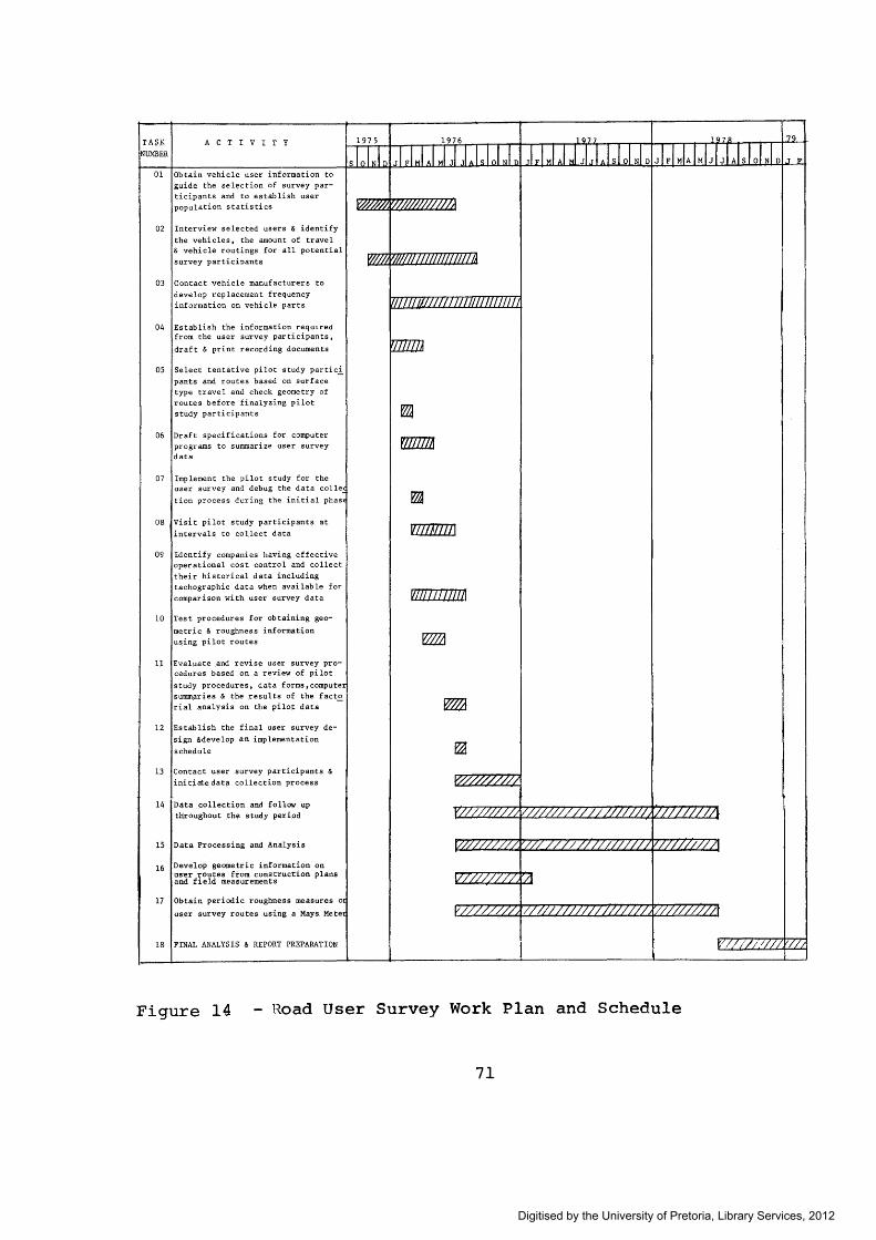
WORK PLAN AND SCHEDULE

The work plan shown in Figure 14 divides the road user

costs surveys into 18 separate activities within the 3 1/2

year period of the project.

In late 1978 a final report will be prepared for this

study; however it is proposed that survey activities should

continue in some for.m to provide additional long term verifi

cation of the results.

Referring to the schedule, there are some major milestone

dates which mark the start or end of key activities.

1) June 1976 marks the end of pre-pilot and pilot studies and finalization of survey design and methodology;

2) In July 1976 the main survey is initiated along with data analysis;

3) In December 1976 the build up to full survey size will be completed;

4) January 1977 marks the completion of initial measurements of vehicle routes and when full definition of the range of route characteristics can be made;

5) July 1978 shows the commencement of final data analysis phase;

6) The Final Report is due in late 1978.

70


TAS.t;

NUMBER A C T I V I T Y

01 Obtain vehicle user information to guide the selection of survey participants and to establish user population statistics

02 Interview selected users & identify

the vehicles, the amount of travel & vehicle routings for all potential

survey participants

03 Contact vehicle manufacturers to

develop replacement frequency information on vehicle parts

04 Establish the information requ1red from the user survey participants,

draft & print recording documents

05 Select tentative pilot study partici_

pants and routes based on surface type travel and check geometry of routes before finalyzing pilot study participants

06 Draft specifications for computer programs to sununarize user survey data

07 Implement the pilot study for the user survey and debug the data colle

tion process dc:ring the initial phasE

08 Visl.t pilot study participants at

intervals to col.lect data

09 Identify companies having effective operational cost control and collect their historical data including tachographic data when available for comparison with user survey data

10 Test procedures for obtaining geo

metric & roughness information using pilot routes

11 Evaluate and revise user survey procedures based on a review of pi lot

study procedures, data forms, computez sunnnaries & the .results of the facto rial analysis on the pilot data

12 Establish the final user survey de

sign &develop an implementation

schedule

13 Contact user survey participants &

initiate data collection process

14 Data collection .and follow up t!iroughout .the study period

15 Data Processing and Analysis

16 Develop geometric information on us·er routes from construction plans and ;field measurements

17 Obtain periodic roughness measures o

user survey routes using a Mays Mete

18 FINAL ANALYSIS & REPORT PREPARATION

1975 1976 1 Q77 1Q7R 7Q

sloiNin JIFIMIJMIJtiJJNin JFIMIAIJJLIIsloiNID JIFIMIAIMLIJIAisloiNID .T F

'///.A

W//J/I////11 I I I II Ill !!In !A

Ill I II Ill I I I I I I I I ITTTTTTl/1!1

-

vzonuwz1

V777//////;V///////// ///////// !/////l/77l

r////////// '/// ////// /J JJJ///JV/7///J// /1

V//////// 'JI

177/7/J/// rJ///////1////////// '/////////Jt

~/// //;1/ //1//

Figure 14 - H.oad User Survey Work Plan and Schedule

71


Documents

CHAPTER 3 ROAD USER COSTS SURVEYS INTRODUCTION