CHAPTER 3 GEOMETRIC DESIGN OF HIGHWAYS

DEPARTMENT OF CIVIL ENGINEERING, AMBO UNVERSITY WOLISO CAMPUS

1 Highway Engineering I Lecture Note

CHAPTER 3

GEOMETRIC DESIGN OF HIGHWAYS

Geometric design is the process whereby the layout of the road in the terrain is designed to meet

the needs of the road users.

3.1 Appropriate Geometric Standards

The needs of road users in developing countries are often very different from those in the

industrialized countries. In developing countries, pedestrians, animal-drawn carts, etc., are often

important components of the traffic mix, even on major roads. Lorries and buses often represent

the largest proportion of the motorized traffic, while traffic composition in the industrialized

countries is dominated by the passenger car. As a result, there may be less need for high-speed

roads in developing countries and it will often be more appropriate to provide wide and strong

shoulders. Traffic volumes on most rural roads in developing countries are also relatively low.

Thus, providing a road with high geometric standards may not be economic, since transport cost

savings may not offset construction costs. The requirements for wide carriageways, flat gradients

and full overtaking sight distance may therefore be inappropriate. Also, in countries with weak

economies, design levels of comfort used in industrialized countries may well be a luxury that

cannot be afforded.

When developing appropriate geometric design standards for a particular road in a developing

country, the first step should normally be to identify the objective of the road project. It is

convenient to define the objective in terms of three distinct stages of development as follows:

Stage 1 – Provision of access

Stage 2 - Provision of additional capacity

Stage 3 – Increase of operational efficiency

Developing countries, by their very nature, will usually not be at stage 3 of this sequence; indeed

most will be at the first stage. However, design standards currently in use are generally

developed for countries at stage 3 and they have been developed for roads carrying relatively

large volumes of traffic. For convenience, these same standards have traditionally been applied

to low-volume roads that lead to uneconomic and technically inappropriate designs.



A study to develop appropriate geometric design standards for use in developing countries has

been undertaken by the Overseas Unit of Transport Research Laboratory (TRL formerly TRRL).

The study revealed that most standards currently in use are considerably higher than can be

justified from an economic or safety point of view. Geometric design recommendations have

been published in Overseas Road Note 6.

In the above-mentioned Overseas Road Note 6 rural access roads are classified into three groups.

Access roads are the lowest level in the network hierarchy. Vehicular flows will be very light

and will be aggregated in the collector road network. Geometric standards may be low and need

only be sufficient to provide appropriate access to the rural agricultural, commercial, and

population centers served. Substantial proportions of the total movements are likely to be by

non-motorized traffic.

Collector roads have the function of linking traffic to and from rural areas, either direct to

adjacent urban centers, or to the arterial road network. Traffic flows and trip lengths will be of an

intermediate level and the need for high geometric standards is therefore less important.

Arterial roads are the main routes connecting national and international centers. Trip lengths are

likely to be relatively long and levels of traffic flow and speed relatively high. Geometric

standards need to be adequate to enable efficient traffic operation under these conditions, in

which vehicle-to-vehicle interactions may be high.

3.2 Design Controls and Criteria

The elements of design are influenced by a wide variety of design controls, engineering criteria,

and project specific objectives. Such factors include the following:

Functional classification of the roadway

Projected traffic volume and composition

Required design speed

Topography of the surrounding land

Capital costs for construction

Human sensory capacities of roadway users

Vehicle size and performance characteristics

Traffic safety considerations



Environmental considerations

Right-of-way impacts and costs

These considerations are not, of course, completely independent of one another. The functional

class of a proposed facility is largely determined by the volume and composition of the traffic to

be served. It is also related to the type of service that a highway will accommodate and the speed

that a vehicle will travel while being driven along a highway.

Of all the factors that are considered in the design of a highway, the principal design criteria are

traffic volume, design speed, sight distances, vehicle size, and vehicle mix.

3.2.1 Design Speed and Design Class

The assumed design speed for a highway may be considered as “ the maximum safe speed that

can be maintained over a specified section of a highway when conditions are so favorable that

the design features govern”. The choice of design speed will depend primarily on the

surrounding terrain and the functional class of the highway. Other factors determining the

selection of design speed include traffic volume, costs of right-of-way and construction, and

aesthetic consideration.

It is therefore recommended that the basic parameters of road function, terrain type and traffic

flow are defined initially. On the basis of these parameters, a design class is selected, while

design speed is used only as an index which links design class to the design parameters of sight

distance and curvature to ensure that a driver is presented with a reasonably consistent speed

environment.

Table 3.1 shows the design classes and design speeds recommended in Overseas Road Note 6 in

relation to road function, volume of traffic and terrain. The table also contains recommended

standards for carriageway and shoulder width and maximum gradient.

The terrain classification as ‘level’, ‘rolling’ or ‘mountainous’ may be defined as average ground

slope measured as the number of five-meter contour lines crossed per kilometer on a straight line

linking the two ends of the road section as follows:

Level terrain: 0 – 10 ground contours per kilometer;



Rolling terrain: 11 – 25 ground contours per kilometer;

Mountainous terrain: > 25 ground contours per kilometer.

Table 3.1 Road design standards (TRRL Overseas Road Note 6)

3.2.2 Sight Distance

The driver’s ability to see ahead contributes to safe and efficient operation of the road. Ideally,

geometric design should ensure that at all times any object on the pavement surface is visible to

the driver within normal eye-sight distance. However, this is not usually feasible because of

topographical and other constraints, so it is necessary to design roads on the basis of lower, but

safe, sight distances.

There are three different sight distances that are of interest in geometric design:

Stopping sight distance;

Meeting sight distance;

Passing sight distance.

Stopping Sight Distance:

The Stopping sight distance comprises two elements: d1 = the distance moved from the instant

the object is sighted to the moment the brakes are applied (the perception and brake reaction

time, referred to as the total reaction time) and d2 = the distance traversed while braking (the

braking distance).

The total reaction time depends on the physical and mental characteristics of the driver,

atmospheric visibility, types and condition of the road and distance to, size color and shape of the



hazard. When drivers are keenly as in urban conditions with high traffic intensity, the reaction

time may be in the range of 0.5 – 1.0 seconds while driver reaction time is generally around 2 – 4

seconds for normal driving in rural conditions. Overseas Road Note 6 assumes a total reaction

time of 2 sec..

The distance traveled before the brakes are applied is:

d1 = 10/36 * V * t

where:

d1 = total reaction distance in m;

V = initial vehicle speed in Km/h

t = reaction time in sec.

The braking distance, d2, is dependent on vehicle condition and characteristics, the coefficient of

friction between tyre and road surface, the gradient of the road and the initial vehicle speed.

d2 = V2 / (254(f + g/100))

where:

d2 = breaking distance in meters;

V = initial vehicle speed in km/h;

f = coefficient of longitudinal friction;

g = gradient( in %; positive if uphill and negative if downhill)

The determination of design values of longitudinal friction, f, is complicated because of the

many factors involved. The design values for longitudinal friction used in Overseas Road Note 6

are shown in table 3.2.

Table 3.2 Coefficient of Longitudinal friction

Design speed

(Km/h)

30

40

50

60

70

85

100

120

f

0.60

0.55

0.50

0.47

0.43

0.40

0.37

0.35

Meeting Sight Distance:

Meeting sight distance is the distance required to enable the drivers of two vehicles traveling in

opposite directions to bring their vehicles to a safe stop after becoming visible to each other.

Meeting sight distance is normally calculated as twice the minimum stopping sight distance.



Passing Sight Distance:

Factors affecting passing (overtaking) sight distance are the judgment of overtaking drivers, the

speed and size of overtaken vehicles, the acceleration capabilities of overtaking vehicles, and the

speed of oncoming vehicles.

Passing sight distances are determined empirically and are usually based on passenger car

requirements. There are differences in various standards for passing sight distance due to

different assumptions about the component distances in which a passing maneuver can be

divided, different assumed speed for the maneuver and, to some extent driver behavior.

The passing sight distances recommended for use by Overseas Road Note 6 are shown in table

3.3.

Table 3.3 Passing sight distances

Design speed

(Km/h)

50 60 70 85 100

120

Passing sight

distance(m)

140 180 240 320 430

590

3.2.3 Traffic Volume

Information on traffic volumes, traffic composition and traffic loading are important factors in

the determination of the appropriate standard of a road. The traffic has a major impact on the

selection of road class, and consequently on all geometric design elements. The traffic

information is furthermore necessary for the pavement design.

For low volume roads the design control is the Average Annual Daily Traffic (AADT) in the

‘design year’. For routes with large seasonal variations the design control is the Average Daily

Traffic (ADT) during the peak months of the ‘design year’. The design year is usually selected as

year 10 after the year of opening to traffic.



3.2.4 Design Vehicle

The dimensions of the motor vehicles that will utilize the proposed facility also influence the

design of a roadway project. The width of the vehicle naturally affects the width of the traffic

lane; the vehicle length has a bearing on roadway capacity and affects the turning radius; the

vehicle height affects the clearance of the various structures. Vehicle weight affects the structural

design of the roadway.

The design engineer will select for design the largest vehicle that is expected to use the roadway

facility in significant numbers on a daily basis.

3.3 Geometric Design Elements

The basic elements of geometric design are: the horizontal alignment, the vertical alignment and

the cross-section. The following elements must be considered when carrying out the geometric

design of a road:

1. Horizontal Alignment:

Minimum curve radius (maximum degree of curvature);

Minimum length of tangent between compound or reverse curves;

Transition curve parameters;

Minimum passing sight distance and stopping sight distance on horizontal curves.

2. Vertical Alignment:

Maximum gradient;

Length of maximum gradient;

Minimum passing sight distance or stopping sight distance on summit (crest)

curves;

Length of sag curves.

3. Cross-section:

Width of carriageway;

Crossfall of carriageway;

Rate of super elevation;

Widening of bends;

Width of shoulder;



Crossfall of shoulder;

Width of structures;

Width of right-of-way;

Sight distance;

Cut and fill slopes and ditch cross-section.

Horizontal and vertical alignment should not be designed independently. They complement each

other and proper combination of horizontal and vertical alignment, which increases road utility

and safety, encourages uniform speed, and improves appearance, can almost always be obtained

without additional costs.

3.3.1 Horizontal Alignment

The horizontal alignment should always be designed to the highest standard consistent with the

topography and be chosen carefully to provide good drainage and minimize earthworks. The

alignment design should also be aimed at achieving a uniform operating speed. Therefore the

standard of alignment selected for a particular section of road should extend throughout the

section with no sudden changes from easy to sharp curvature. Where a sharp curvature is

unavoidable, a sequence of curves of decreasing radius is recommended.

The horizontal alignment consists of a series of intersecting tangents and circular curves, with or

without transition curves.

3.3.1.1 Straights (Tangents)

Long straights should be avoided, as they are monotonous for drivers and cause headlight dazzle

on straight grades. A more pleasing appearance and higher road safety can be obtained by a

winding alignment with tangents deflecting some 5 – 10 degrees alternately to the left and right.

Short straights between curves in the same direction should not be used because of the broken

back effect. In such cases where a reasonable tangent length is not attainable, the use of long,

transitions or compound curvature should be considered.

The following guidelines may be applied concerning the length of straights:



Straights should not have lengths greater than (20 * V) meters, where V is the design

speed in km/h.

Straights between circular curves turning in the same direction should have lengths

greater than (6*V) meters, where V is the design speed in km/h.

Straights between the end and the beginning of untransitioned reverse circular curves

should have lengths greater than two-thirds of the total superelevation run-off.

3.3.1.2 Circular Curves

Horizontal curvature design is one of the most important features influencing the efficiency and

safety of a highway. Improper design will result in lower speeds and lowering of highway

capacity.

Figure 3.1: Parts of a Circular Curve

Note:

PC – point of curvature



PI – point of intersection

PT – point of tangency

Δ – central angle

R – radius of curve

D – degree of curve that defines,

a. Central angle which subtends 20m arc (arc definition),

b. Central angle which subtends 20m chord (Chord definition)

From arc definition,

R = 1145.916 / D

From chord definition,

R = 10 / Sin (D/2)

Tangent (T): distance from PC to PI(backward tangent) or from PT to PI(forward

tangent)

T = R*tan (Δ/2)

External distance (E): distance from PI to middle of curve.

E = R*(Sec (Δ/2) – 1 or E = T*tan (Δ/4)

Middle ordinate (M): length from the middle of chord to the middle of curve.

M = R*(1- Cos (Δ/2))

Long chord(C): straight-line distance from A to B.

C = 2R*Sin (Δ/2)

Length of Curve (Lc): distance from PC to PT along the curve.

Lc = 20* Δ/D or Lc = R*π* Δ/180

Sub-arc angles di: are angles subtended by an arc less than the degree of curve (D).

di = Ai*D/20

where:



di = angle subtended by sub-arc of length Ai

Ai = arc less than 20m.

Sub chord angle (dj): are angles subtended by a chord less than the degree of curve (D).

cj = 2R*Sin(dj/2)

Also

cj = 20Sin(dj/2)/Sin(D/2)

Where:

dj = angle subtended by sub-chord of length cj

cj = chord less than 20m.

Deflection angles: The angle that a chord deflects from a tangent to a circular curve is

measured by half of the intercepted arc.

o Deflection angle for Lc m = Δ/2

o Deflection angle for 20m = D/2

o Deflection angle for Ai m = di/2

Stations of PC, PI, and PT:

PC = PI – T

P T = PC + Lc or PT = PI + T

Several variations of the circular curve deserve consideration when developing the horizontal

alignment for a highway design. When two curves in the same direction are connected with a

short tangent, this condition is referred to as a “broken back” arrangement of curves. This type of

alignment should be avoided except where very unusual topographical or right-of-way

conditions dictate otherwise. Highway engineers generally consider the broken back alignment to

be unpleasant and awkward and prefer spiral transitions or a compound curve alignment with

continuous superelvation for such conditions.

Figure 3.2 identifies elements of a typical compound highway curve with variable definitions and

basic equations developed for a larger and smaller radius curve, based on the assumption that the



radius dimensions RL and RS and central angles ΔL and ΔS are given or have been previously

determined.

Figure 3.2 Properties of a Compound Curve

Another important variation of the circular highway curve is the use of reverse curves, which are

adjacent curves that curve in opposite directions. The alignment illustrated in figure 3.3, which

shows a point of reverse curvature, PRC, and no tangent separating the curves, would be suitable

only for low-speed roads such as those in mountainous terrain. A sufficient length of tangent



between the curves should usually be provided to allow removal of the superelevation from the

first curve and attainment of adverse superelevation for the second curve.

Figure 3.3 Properties of a Reverse Curve



Sight Distance on Horizontal Curves:

(a) (b)

Figure 3.4 Sight Distance Around Horizontal Curve: (a) S < Lc and (b) S > Lc

Situations frequently exist where an object on the inside of a curve, such as vegetation, building

or cut face, obstructs the line of sight. Where it is either not feasible or economically justified to

move the object a larger radius of curve will e required to ensure that stopping sight distance is

available. The required radius of curve is dependent on the distance of the obstruction from the

centerline and the sight distance.

Case 1. S < Lc

S = 40 * Cos-1 ((R-M)/R) / D

Case 2. S > Lc

M = Lc* (2S - Lc) / 8R

Night driving around sharp curves introduces an added problem related to horizontal sight

distance. Motor-vehicle headlights are pointed directly toward the front and do not provide as

much illumination in oblique directions. Even if adequate horizontal sight distance is provided, it



has little useful purpose at night because the headlights are directed along a tangent to the curve,

and the roadway itself is not properly illuminated.

3.3.1.3 Superelevation

Figure 3.5 Forces acting on a vehicle moving

along a curved path.

When velocity v(m/s) is stated in V(Km/h), and the radius of curve(R) in meters, the equation

reduces to

f = V2 / (127*R)

On highway curves, this centrifugal force acts through the center of mass of the vehicle and

creates an overturning moment about the points of contact between the outer wheels and the

pavement. But a stabilizing (resisting) moment is created by the weight acting through the center

of mass. Thus for equilibrium conditions,

(m * v2 / R) * h = m * g * d/2

and

h = d / (2v2 / gR) = d / 2f

where

Any body moving rapidly along a curved

path is subject to an outward reactive force

called the centrifugal force. If the surface is

flat, the vehicle is held in the curved path

by side friction between tires and

pavement. The total of these friction forces

balances the centrifugal force. Expressed in

terms of the coefficient of friction f and the

normal forces between the pavement and

the tires, the relationship is

m *v2/R = (NL + NR)*f = m*g*f

or

f = v2 / ( g * R)



h = height of the center of mass above pavement

d = lateral width between the wheels

For the moment equation, if f = 0.5, then the height to the center of mass must be greater than the

lateral distance between the wheels before overturning will take place. Modern passenger

vehicles have low center of mass so that relatively high values of f have to be developed before

overturning would take place. In practice, the frictional value is usually sufficiently low for

sliding to take place before overturning. It is only with certain commercial vehicles having high

center of mass that the problem of overturning may arise.

In order to resist the outward acting centrifugal force, and to enable vehicles to round curves at

design speed without discomfort to their occupants, the pavements are “tilted” or

“superelevated” so that the outer edges are higher than the inner edges. This tilting, plus

frictional resistance between the tires and the pavement provides a horizontal resistance to the

centrifugal forces generated by the circular movement of the vehicle around a curve.

Analysis of the forces acting on a vehicle as it moves around a curve of constant radius indicates

that the theoretical superelevation can be expressed as:

e + f = V2 / (127*R) ……………………………………………(*)

where:

e = rate of superelevation(m per m)

f = side friction factor (or coefficient of lateral friction)

V = speed (Km/hr)

R = radius of curvature (m)

Equation (*) above is the basic equation relating the speed of vehicles, the radius of curve, the

superelevation and the coefficient of lateral friction. This equation forms the basis of design of

horizontal curves.



If the entire centrifugal force is counteracted by the superelevation, frictional force will not be

called into play. Proper design does not normally take full advantage of the obtainable lateral

coefficients of friction, since the design should not be based on a condition of incipient sliding.

In design, engineers use only a portion of the friction factor, accounting for the comfort and

safety of the vast majority of drivers.

From equation (*), the minimum radius or maximum degree of curvature for a given design

speed can be determined from the rate of superelevation and side friction factor.

R = V2 / (127*(e + f))

D = 1145.916 / R

Attainment of Superelevation:

The transition from a tangent, normal crown section to a curved superelevated section must be

accompanied without any appreciable reduction in speed and in such a manner as to ensure

safety and comfort to the occupants of the traveling vehicle.

The normal cambered surface on a straight reach of road is changed into a superelevated surface

into two stages. In the first stage, the outer half of the camber is gradually raised until it is level.

In the second stage, three methods may be adopted to attain the full super-elevation.

i. The surface of the road is rotated about the centerline of the carriageway, gradually

lowering the inner edge and raising the upper edge, keeping the level of the centerline

constant.

ii. The surface of the road is rotated about the inner edge, raising the center and the outer

edge.

iii. The surface of the road is rotated about the outer edge depressing the center and the outer

edge.

Method (i) is the most generally used.



The distance required for accomplishing the transition from a normal to a superelevated section,

commonly referred to as the transition runoff, is a function of the design speed and the rate of

superelevation.

Superelevation is usually started on the tangent at some distance before the curve starts, and the

full superelevation is generally reached beyond the point of curvature (PC) of the curve. In

curves with transitions, the superelevation can be attained within the limits of the spiral.

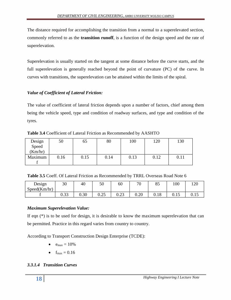
Value of Coefficient of Lateral Friction:

The value of coefficient of lateral friction depends upon a number of factors, chief among them

being the vehicle speed, type and condition of roadway surfaces, and type and condition of the

tyres.

Table 3.4 Coefficient of Lateral Friction as Recommended by AASHTO

Design

Speed

(Km/hr)

50 65 80 100 120 130

Maximum

f

0.16 0.15 0.14 0.13 0.12 0.11

Table 3.5 Coeff. Of Lateral Friction as Recommended by TRRL Overseas Road Note 6

Design

Speed(Km/hr)

30 40 50 60 70 85 100 120

f 0.33 0.30 0.25 0.23 0.20 0.18 0.15 0.15

Maximum Superelevation Value:

If eqn (*) is to be used for design, it is desirable to know the maximum superelevation that can

be permitted. Practice in this regard varies from country to country.

According to Transport Construction Design Enterprise (TCDE):

emax = 10%

fmax = 0.16

3.3.1.4 Transition Curves



Transition curves provide a gradual change from the tangent section to the circular curve and

vice versa. For most curves, drivers can follow a transition path within the limits of a normal

lane width, and a spiral transition in the alignment is not necessary. However, along high-speed

roadways with sharp curvature, transition curves may be needed to prevent drivers from

encroaching into adjoining lanes.

A curve known as the Euler spiral or clothoid is commonly used in highway design. The radius

of the spiral varies from infinity at the tangent end to the radius of the circular arc at the end of

the spiral. The radius of the spiral at any point is inversely proportional to the distance from its

beginning point.

Figure 3.6 Main Elements of A Circular Curve Provided with Transitions

Some of the important properties of the spirals are given below:

L = 2Rθ

θ = (L / Ls)2 * θs

θs = Ls / 2Rc (in radians) = 28.65Ls / Rc (in degrees)

Ts = Ls /2 + (Rc + S)*tan(Δ/2)



S = Ls2 / 24Rc

Es = (Rc + S)*sec(Δ/2) - Rc

Note:

θs = spiral angle

Δ = total central angle

Δc = central angle of the circular arc extending from BC to EC = Δ - 2 θs

Rc = radius of circular curve

L = length of spiral from starting point to any point

R = radius of curvature of the spiral at a point L distant from starting

point.

Ts = tangent distance

Es = external distance

S = shift

HIP = horizontal intersection point

BS = beginning of spiral

BC = beginning of circular curve

EC = end of circular curve

ES = end of spiral curve

Length of Transition:

The length of transition should be determined from the following two conditions:

The rate of change of centrifugal acceleration adopted in the design should not cause

discomfort to the drivers. If C is the rate of change of acceleration,

Ls = 0.0215V3 / (C*Rc)

Where:

V = speed (Km/hr)

Rc = radius of the circular curve (m)

The rate of change of superelevation (superelevation application ratio) should be such as

not to cause higher gradients and unsightly appearances. Since superelevation can be



given by rotating about the centerline, inner edge or outer edge, the length of the

transition will be governed accordingly.

3.3.1.5 Widening of Curves

Extra width of pavement may be necessary on curves. As a vehicle turns, the rear wheels follow

the front wheels on a shorter radius, and this has the effect of increasing the width of the vehicle

in relation to the lane width of the roadway. Studies of drivers traversing curves have shown that

there is a tendency to drive a curved path longer than the actual curve, shifting the vehicle

laterally to the right on right-turning curves and to the left on left-turning curves. Thus, on right-

turning curves the vehicle shifts toward the inside edge of the pavement, creating a need for

additional pavement width. The amount of widening needed varies with the width of the

pavement on tangent, the design speed, and the curve radius or degree of curvature.

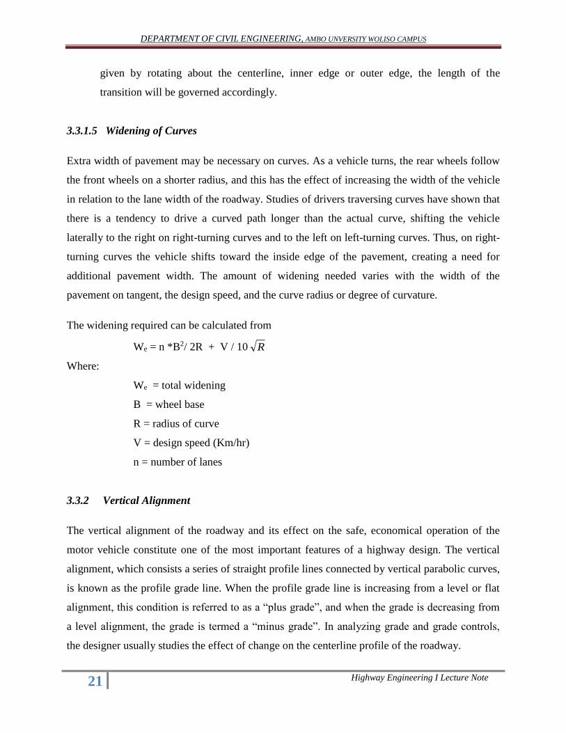
The widening required can be calculated from

We = n *B2/ 2R + V / 10 R

Where:

We = total widening

B = wheel base

R = radius of curve

V = design speed (Km/hr)

n = number of lanes

3.3.2 Vertical Alignment

The vertical alignment of the roadway and its effect on the safe, economical operation of the

motor vehicle constitute one of the most important features of a highway design. The vertical

alignment, which consists a series of straight profile lines connected by vertical parabolic curves,

is known as the profile grade line. When the profile grade line is increasing from a level or flat

alignment, this condition is referred to as a “plus grade”, and when the grade is decreasing from

a level alignment, the grade is termed a “minus grade”. In analyzing grade and grade controls,

the designer usually studies the effect of change on the centerline profile of the roadway.



In the establishment of a grade, an ideal situation is one in which the cut is balanced against the

fill without a great deal of borrow or an excess of cut material to be wasted. All earthwork hauls

should be moved in a downhill direction if possible and within a relatively short distance from

the origin, due to the expense of moving large quantities of soil. Ideal grades have long distances

between points of intersection, with long curves between grade tangents to provide smooth riding

qualities and good visibility. The grade should follow the general terrain and rise or fall in the

direction of the existing drainage. In rock cuts and in flat, low-lying or swampy areas, it is

necessary to maintain higher grades with respect to the existing ground line. Future possible

construction and the presence of grade separations or bridge structures can also act as control

criteria for the design of a vertical alignment.

3.3.2.1 Grades and Grade Control

Changes of grade from plus to minus should be placed in cuts, and changes from a minus grade

to a plus grade should be placed in fills. This will generally give a good design, and many times

it will avoid the appearance of building hills and producing depressions contrary to the general

existing contours of the land. Other considerations for determining the grade line may be of more

importance than the balancing of cuts and fills.

In the analysis of grades and grade control, one of the most important considerations is the effect

of grades on the operating costs of the motor vehicle. An increase in gasoline consumption, a

reduction in speed, and an increase in emissions and noise are apparent when grades are

increased. An economical approach would be to balance the added cost of grade reduction

against the annual costs and impacts of vehicle operation without grade reduction. An accurate

solution to the problem depends on the knowledge of traffic volume and type, which can be

obtained by means of a traffic survey.

Minimum grades are governed by drainage conditions. Level grades may be used in fill sections

in rural areas when crowned pavements and sloping shoulders can take care of the pavement

surface drainage. However, it is preferred that the profile grade be designed to have a minimum

grade of at least 0.3 percent under most conditions in order to secure adequate drainage.



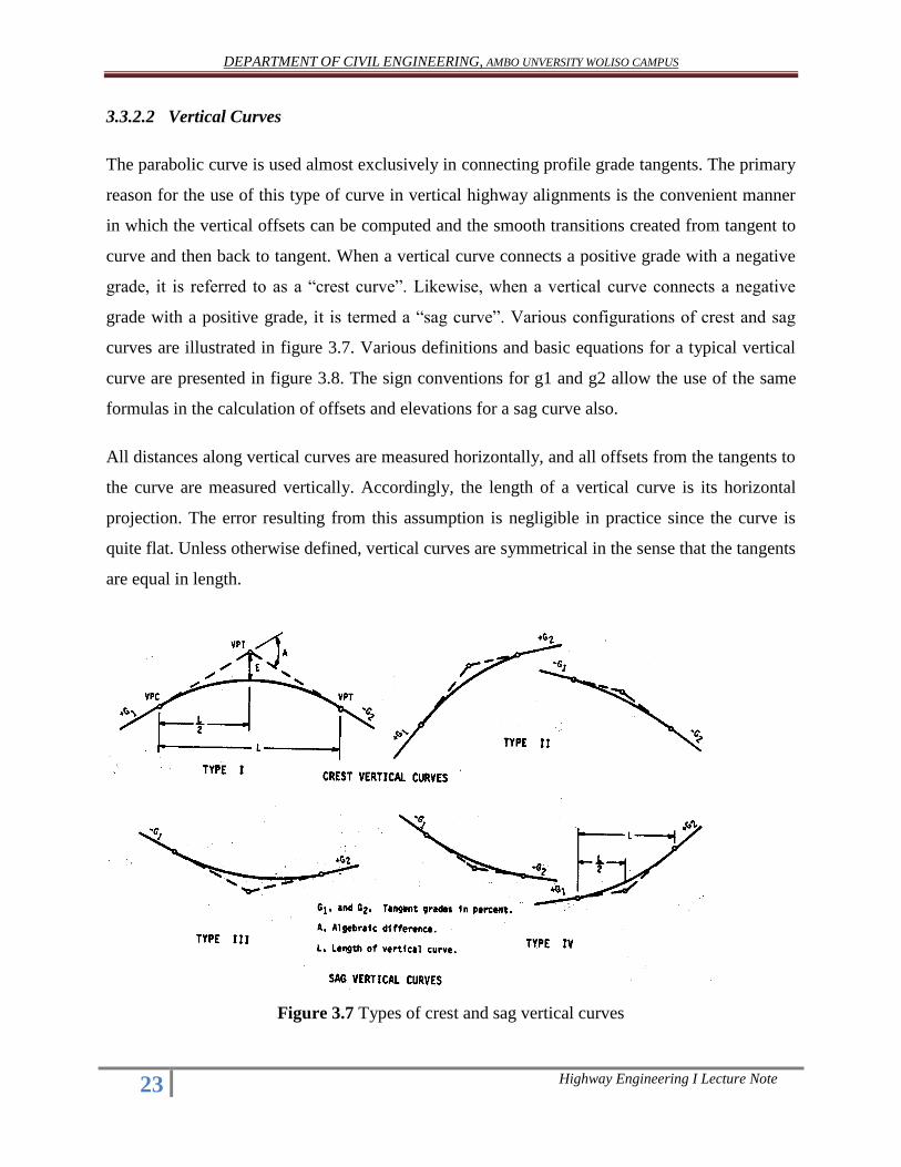
3.3.2.2 Vertical Curves

The parabolic curve is used almost exclusively in connecting profile grade tangents. The primary

reason for the use of this type of curve in vertical highway alignments is the convenient manner

in which the vertical offsets can be computed and the smooth transitions created from tangent to

curve and then back to tangent. When a vertical curve connects a positive grade with a negative

grade, it is referred to as a “crest curve”. Likewise, when a vertical curve connects a negative

grade with a positive grade, it is termed a “sag curve”. Various configurations of crest and sag

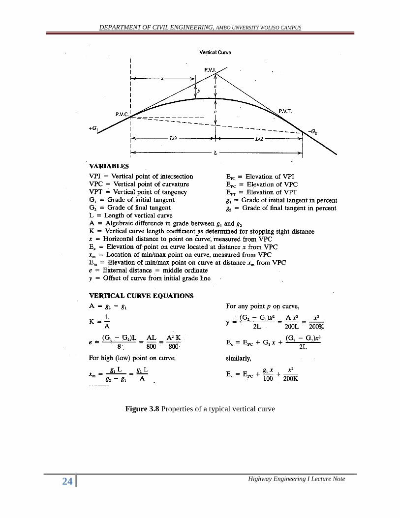
curves are illustrated in figure 3.7. Various definitions and basic equations for a typical vertical

curve are presented in figure 3.8. The sign conventions for g1 and g2 allow the use of the same

formulas in the calculation of offsets and elevations for a sag curve also.

All distances along vertical curves are measured horizontally, and all offsets from the tangents to

the curve are measured vertically. Accordingly, the length of a vertical curve is its horizontal

projection. The error resulting from this assumption is negligible in practice since the curve is

quite flat. Unless otherwise defined, vertical curves are symmetrical in the sense that the tangents

are equal in length.

Figure 3.7 Types of crest and sag vertical curves



Figure 3.8 Properties of a typical vertical curve



3.3.2.3 Length Of Vertical Curves

A. Crest Curves:

For crest curves, the most important consideration in determining the length of the curve

is the sight distance requirement.

Case1: S < L

Case 2: S > L

AASHTO recommendations:

For stopping sight distance over crest: h1 = 1.07m and h2 = 0.15m

For passing sight distance over crest: h1 = 1.07m and h2 = 1.30m

B. Sag Curves:

For sag curves, the criteria for determining the length are vehicle headlight distance, rider

comfort, drainage control and general appearance.

2

21

2

)22( hh

GSL

G

hhSL

2

21 )(2*2



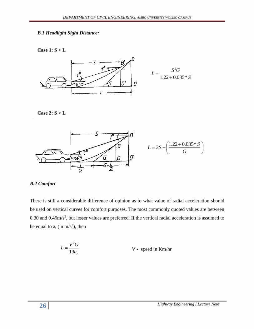
B.1 Headlight Sight Distance:

Case 1: S < L

Case 2: S > L

B.2 Comfort

There is still a considerable difference of opinion as to what value of radial acceleration should

be used on vertical curves for comfort purposes. The most commonly quoted values are between

0.30 and 0.46m/s2, but lesser values are preferred. If the vertical radial acceleration is assumed to

be equal to ar (in m/s2), then

ra

GVL

13

2

S

GSL

*035.022.1

2

G

SSL

*035.022.12

V - speed in Km/hr



3.3.2.4 Sight Distances At Underpass Structures:

Case 1: S < L

Case 2: S > L

AASHTO recommendations: h1 = 1.829m, h2 = 0.457m and C = 5.182m

3.3.3 Cross-Section

The cross-sectional elements in a highway design pertain to those features that deal with its

width. They embrace aspects such as right-of-way, roadway width, central reservations

(medians), shoulders, camber, side-slope etc.

Right- Of –Way

The right-of-way width is the width of land secured and preserved to the public for road

purposes. The right-of-way should be adequate to accommodate all the elements that make up

the cross-section of the highway and may reasonably provide for future development.

m

GSL

8

2

Where:

m = C – (h1+h2)/2

C = Vertical clearance distance

G

mSL

82



Road Width

Road width should be minimized so as to reduce the costs of construction and maintenance,

whilst being sufficient to carry the traffic loading efficiently and safely.

The following factors need to be taken into account when selecting the width of a road:

1. Classification of the road. A road is normally classified according to its function in the

road network. The higher the class of road, the higher the level of service expected and

the wider the road will need to be.

2. Traffic. Heavy traffic volumes on a road mean that passing of oncoming vehicles and

overtaking of slower vehicles are more frequent and therefore that paths of vehicles will

be further from the center-line of the road and the traffic lanes should be wider.

3. Vehicle dimensions. Normal steering deviations and tracking errors, particularly of

heavy vehicles, reduce clearances between passing vehicles. Higher truck percentages

require wider traffic lanes.

4. Vehicle speed. As speeds increase, drivers have less control of the lateral position of

vehicles, reducing clearances, and so wider traffic lanes are needed.

Figure 3.9 shows the typical cross-sections recommended by Overseas Road Note 6, for the

various road design classes A – F.

The cross-section of the road is usually maintained across culverts, but special cross-sections

may need to be designed for bridges, taking into account traffic such as pedestrians, cyclists, etc.,

as well as motor traffic. Reduction in the carriageway width may be accepted, for instance, when

an existing narrow bridge has to be retained because it is not economically feasible to replace or

widen it. It may also sometimes be economic to construct a superstructure of reduced width

initially with provision for it to be widened later when traffic warrants it. In such cases a proper

application of traffic signs, rumble strips or speed bumps is required to warn motorists of the

discontinuity in the road.



Figure 3.9 Typical cross-sections (TRRL Overseas Road Note 6)



For single-lane roads without shoulders passing places must be provided to allow passing and

overtaking. The total road width at passing places should be a minimum of 5.0m but preferably

5.5m, which allows two trucks to pass safely at low speed. The length of individual passing

places will vary with local conditions and the sizes of vehicles in common use but, generally, a

length of 20m including tapers will cater for trucks with a wheelbase of 6.5m and an overall

length of 11.0m.

Normally, passing places should be located every 300-500m depending on the terrain and

geometric conditions. They should be located within sight distance of each other and be

constructed at the most economic locations as determined by terrain and ground conditions, such

as at transitions from cut to fill, rather than at precise intervals.

Shoulders

Shoulders provide for the accommodation of stopped vehicles. Properly designed shoulders also

provide an emergency outlet for motorists finding themselves on a collision course and they also

serve to provide lateral support to the carriageway. Further, shoulders improve sight distances

and induce a sense of ‘openness’ that improves capacity and encourages uniformity of speed.

In developing countries shoulders are used extensively by non-motorized traffic (pedestrians,

bicycles and animals) and a significant proportion of the goods may be transported by such non-

motorized means.

Cross-Fall

Two-lane roads should be provided with a camber consisting of a straight-line cross-fall from the

center-line to the carriageway edges, while straight cross-fall from edge to edge of the

carriageway is used for single-lane roads and for each carriageway of divided roads.

The cross-fall should be sufficient to provide adequate surface drainage whilst not being so great

as to be hazardous by making steering difficult. The ability of a surface to shed water varies with

its smoothness and integrity. On unpaved roads, the minimum acceptable value of cross-fall

should be related to the need to carry surface water away from the pavement structure



effectively, with a maximum value above which erosion of a material starts to become a

problem.

According to Overseas Road Note 6 the normal cross-fall should be 3% on paved roads and 4 –

6% on unpaved roads.

Due to the action of traffic and weather the cross-fall of unpaved roads will gradually be reduced

and rutting may develop. To avoid the rutting developing into potholes a cross-fall of 5 – 6%

should be reestablished during the routine and periodic maintenance works.

Shoulders having the same surface as the carriageway should have the same cross-slope.

Unpaved shoulders on a paved road should be about 2% steeper than the cross-fall of the

carriageway.

Side Slopes

The slopes of fills (embankments) and cuts must be adapted to the soil properties, topography

and importance of the road. Earth fills of common soil types and usual height may stand safely

on slopes of 1 on 1.5 and slopes of cuts through undisturbed earth with cementing properties

remain in place with slopes of about 1 on 1. Rock cuts are usually stable at slopes of 4 on 1 or

even steeper depending on the homogeneity of the rock formation and direction of possible dips

and strikes.

Using these relatively steep slopes will result in minimization of earthworks, but steep slopes are,

on the other hand, more liable to erosion than flatter slopes as plant and grass growth is

hampered and surface water velocity will be higher. Thus the savings in original excavation and

embankment costs may be more than offset by increased maintenance through the years.



ASSIGNMENT_3

In a design of an arterial highway, a 2.5% descending grade intersects a 3% ascending grade. The starting of a symmetrical parabolic curve, PVC that joins these two grades is at station 9 + 600 and elevation 1325.75 m. It is proposed to locate the lowest point on the curve at the proposed cross drainage structure, at station 9 + 672.727 and elevation 1324.84 m. For a design speed of 80 Km/hr; perception reaction time = 2.5 sec; and coefficient of friction = 0.3:

a. Determine the length of the curve that passes through the lowest

point. b. Does the curve length determined in (a) satisfy the requirements of

minimum stopping sight distance and comfort? If not, what should be the curve length satisfying these requirements.

c. Calculate the elevations on the curve at stations 9+640 and 9+740 assuming a curve length of 180 m.

Documents

CHAPTER 3 GEOMETRIC DESIGN OF HIGHWAYS