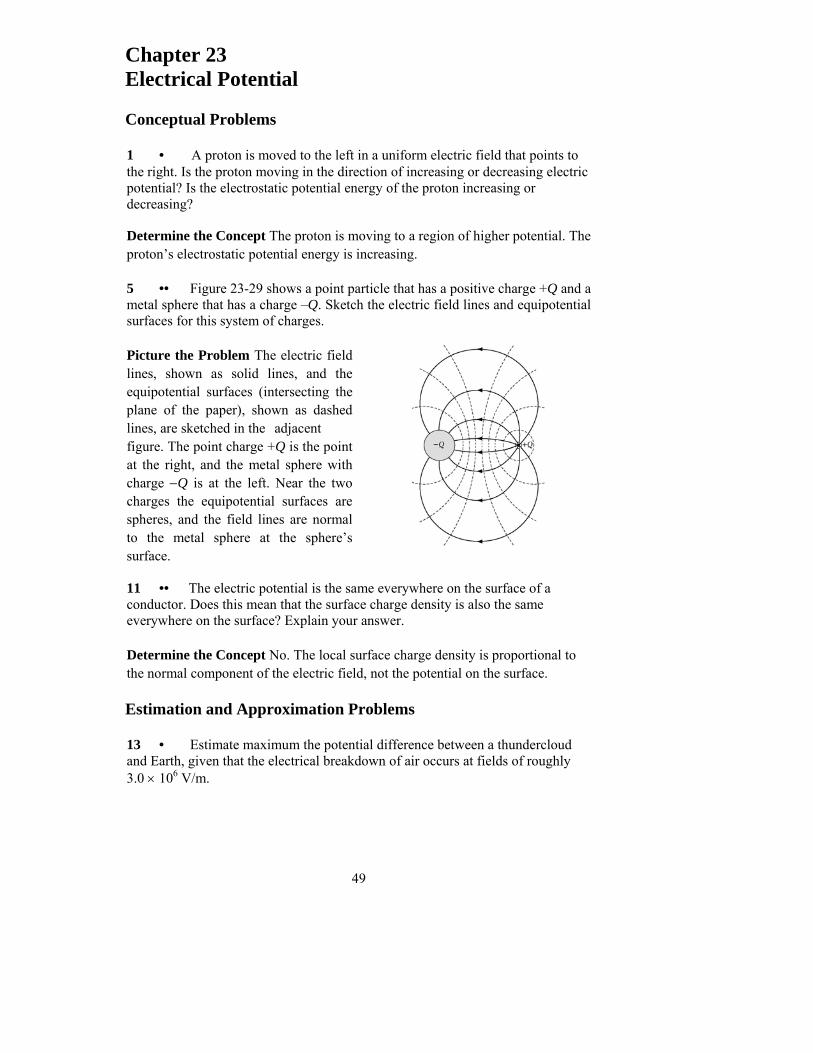
Chapter 23 Electrical Potential Conceptual Problems 1 • A proton is moved to the left in a uniform electric field that points to the right. Is the proton moving in the direction of increasing or decreasing electric potential? Is the electrostatic potential energy of the proton increasing or decreasing? Determine the Concept The proton is moving to a region of higher potential. The proton’s electrostatic potential energy is increasing. 5 •• Figure 23-29 shows a point particle that has a positive charge +Q and a metal sphere that has a charge –Q. Sketch the electric field lines and equipotential surfaces for this system of charges. Picture the Problem The electric field lines, shown as solid lines, and the equipotential surfaces (intersecting the plane of the paper), shown as dashed lines, are sketched in the adjacent figure. The point charge +Q is the point at the right, and the metal sphere with charge −Q is at the left. Near the two charges the equipotential surfaces are spheres, and the field lines are normal to the metal sphere at the sphere’s surface.

11 •• The electric potential is the same everywhere on the surface of a conductor. Does this mean that the surface charge density is also the same everywhere on the surface? Explain your answer. Determine the Concept No. The local surface charge density is proportional to the normal component of the electric field, not the potential on the surface. Estimation and Approximation Problems 13 • Estimate maximum the potential difference between a thundercloud and Earth, given that the electrical breakdown of air occurs at fields of roughly 3.0 × 106 V/m.

49

Chapter 23

50

EdV

Picture the Problem Picture the Problem The potential difference between the thundercloud and Earth is the product of the electric field between them and their separation. Express the potential difference between the cloud and Earth as a function of their separation d and electric field E between them:

=

Assuming that the thundercloud is at a distance of about 1 km above the surface of Earth, the potential difference is approximately:

( )( )V100 9×.3

m10V/m100.3 36

=

×=V

fKKW

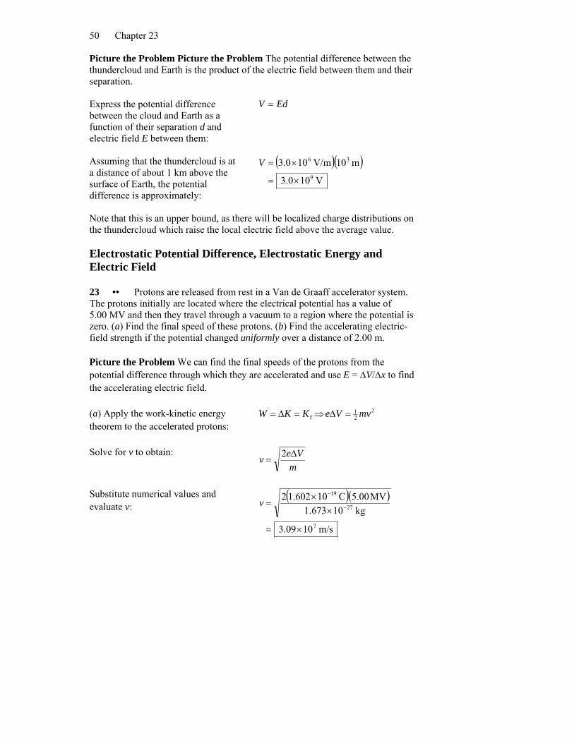
Note that this is an upper bound, as there will be localized charge distributions on the thundercloud which raise the local electric field above the average value. Electrostatic Potential Difference, Electrostatic Energy and Electric Field 23 •• Protons are released from rest in a Van de Graaff accelerator system. The protons initially are located where the electrical potential has a value of 5.00 MV and then they travel through a vacuum to a region where the potential is zero. (a) Find the final speed of these protons. (b) Find the accelerating electric-field strength if the potential changed uniformly over a distance of 2.00 m. Picture the Problem We can find the final speeds of the protons from the potential difference through which they are accelerated and use E = ΔV/Δx to find the accelerating electric field. (a) Apply the work-kinetic energy theorem to the accelerated protons:

=Δ= ⇒ 221 mvVe =Δ

Solve for v to obtain: m

Vev Δ=

2

Substitute numerical values and evaluate v:

( )( )

m/s1009

101.6737

27

×

× −

.3

kgMV5.00C101.6022 19

=

×=

−

v

Electric Potential

51

(b) Assuming the same potential change occurred uniformly over the distance of 2.00 m, we can use the relationship between E, ΔV, and Δx express and evaluate E:

MV/m2.50m2.00

MV5.00==

ΔΔ

=xVE

Potential Due to a System of Point Charges 27 • Three point charges are fixed at locations on the x axis: q1 is at x = 0.00 m, q2 is at x = 3.00 m, and q3 is at x = 6.00 m. Find the electric potential at the point on the y axis at y = 3.00 m if (a) q1 = q2 = q3 = +2.00 μC, (b) q1 = q2 = +2.00 μC and q3 = –2.00 μC, and (c) q1 = q3 = +2.00 μC and q2 = –2.00 μC. (Assume the potential is zero very far from all charges.) Picture the Problem The potential at the point whose coordinates are (0, 3.00 m) is the algebraic sum of the potentials due to the charges at the three locations given. Express the potential at the point whose coordinates are (0, 3.00 m): ⎟⎟

⎠

⎞⎜⎜⎝

⎛++== ∑

= 3

3

2

2

1

13

1 rq

rq

rqk

rqkV

i i

i

( )( )

(a) For q1 = q2 = q3 = 2.00 μC:

kV9.12

m53.00m23.00m3.001C00.2/CmN10988.8 229

=

⎟⎟⎠

⎜⎜⎝

⎛++⋅×= μV

( )( )

11 ⎞

(b) For q1 = q2 = 2.00 μC and q3 = −2.00 μC:

kV55.7

m53.001

m23.001

m3.001C00.2/CmN10988.8 229

=

⎟⎟⎠

⎞⎜⎜⎝

⎛−+⋅×= μV

(c) For q1 = q3 = 2.00 μC and q2 = −2.00 μC:

( )( )

kV43.4=

Vm53.00

1m23.00

1m3.00

1C00.2/CmN10988.8 229⎟⎟⎠

⎞⎜⎜⎝

⎛+−⋅×= μ

Chapter 23

52

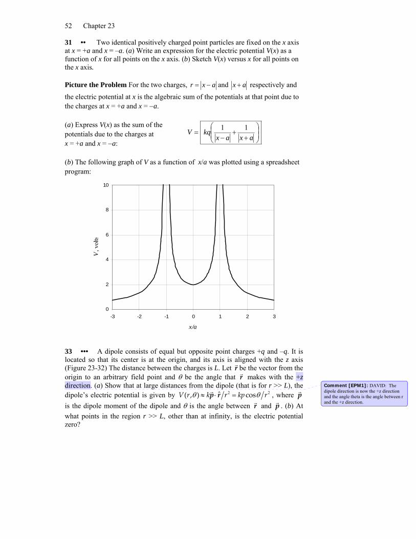
31 •• Two identical positively charged point particles are fixed on the x axis at x = +a and x = –a. (a) Write an expression for the electric potential V(x) as a function of x for all points on the x axis. (b) Sketch V(x) versus x for all points on the x axis. Picture the Problem For the two charges, axr −= and ax + respectively and

the electric potential at x is the algebraic sum of the potentials at that point due to the charges at x = +a and x = −a. (a) Express V(x) as the sum of the potentials due to the charges at x = +a and x = −a:

⎟⎠

⎜⎝ +− axax

⎟⎞

⎜⎛

+= kqV 11

(b) The following graph of V as a function of x/a was plotted using a spreadsheet program:

0

2

4

6

8

-3 -2 -1 0 1 2 3

x/a

V, v

olt

10

s

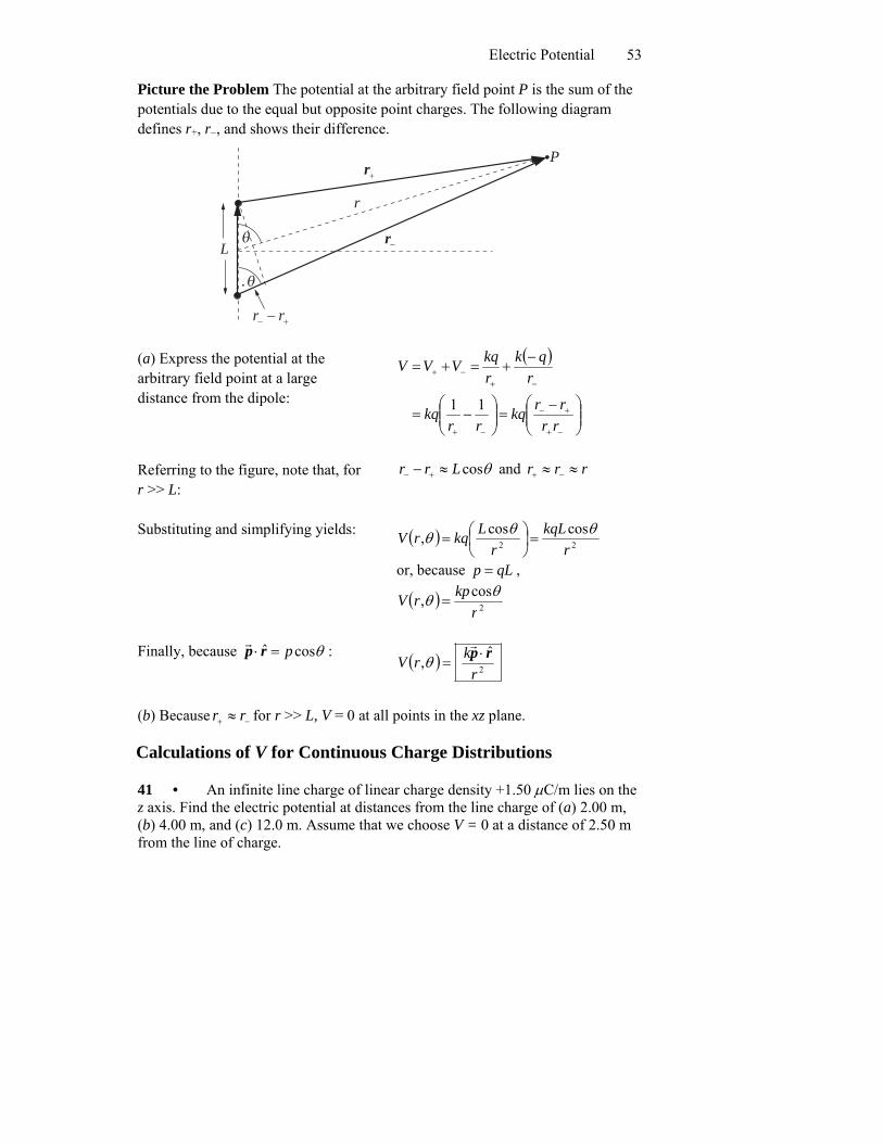
33 ••• A dipole consists of equal but opposite point charges +q and –q. It is located so that its center is at the origin, and its axis is aligned with the z axis (Figure 23-32) The distance between the charges is L. Let rr be the vector from the origin to an arbitrary field point and θ be the angle that rr makes with the +z direction. (a) Show that at large distances from the dipole (that is for r >> L), the dipole’s electric potential is given by 2 2θ θ≈ ⋅ =

r ˆ( , ) cosk r kp rp r rpV r , where is the dipole moment of the dipole and θ is the angle between rr and rp . (b) At what points in the region r >> L, other than at infinity, is the electric potential zero?

Comment [EPM1]: DAVID: The dipole direction is now the +z direction and the angle theta is the angle between r and the +z direction.

Electric Potential

53

Picture the Problem The potential at the arbitrary field point P is the sum of the potentials due to the equal but opposite point charges. The following diagram defines r+, r−, and shows their difference.

+rr

−rrθ

+− − rr

L

θ.

P

r

( )−(a) Express the potential at the arbitrary field point at a large distance from the dipole: ⎟⎟

⎠

⎞⎜⎜⎝

⎛ −=⎟⎟

⎠

⎞−⎜⎜

⎝

⎛=

+=+=−+

−+

kq

rqk

rkqVVV

−+

+−

−+ rrrrkq

rr11

Referring to the figure, note that, for r >> L:

θcosLrr − ≈+− rr and r ≈ ≈−+

( )

Substituting and simplifying yields: 2

cos,r

rV θθ =⎟⎠⎞

⎜⎝⎛=

qLp

2

cos kqLr

Lkq θ

or, because = ,

( ) 2cos,r

kprV θθ =

Finally, because θcosˆ p=⋅ rpr ( ): 2r

=ˆ

, krV rp ⋅r

θ

−+ ≈ r

(b) Because r for r >> L, V = 0 at all points in the xz plane. Calculations of V for Continuous Charge Distributions 41 • An infinite line charge of linear charge density +1.50 μC/m lies on the z axis. Find the electric potential at distances from the line charge of (a) 2.00 m, (b) 4.00 m, and (c) 12.0 m. Assume that we choose V = 0 at a distance of 2.50 m from the line of charge.

Chapter 23

54

Picture the Problem We can use the expression for the potential due to a line

charge ( ) ⎟⎠⎞

⎜⎝⎛−=

arkr ln2 λ

( )

V , where V = 0 at some distance r = a, to find the

potential at these distances from the line. Express the potential due to a line charge as a function of the distance from the line:

⎟⎠

⎜⎝ a

k ln2 λ ⎞⎛−=rrV

Because V = 0 at r = 2.50 m: ⎟⎞

⎜⎛−= k m50.2ln20 λ

⎠⎝ a

Equivalently:

⎟⎠⎞

⎜⎝⎛=

am50.2ln0 ⇒ ( ) 10lnm50.2 1 == −

a

( )

Solving for a gives: a = 2.50 m

Thus we have a = 2.50 m and:

( ) ⎟⎟⎠

⎞⎜⎜⎝

⎛⋅×−=

m50.2lnm/CN10696.2 4 r

⎟⎟⎠

⎞⎜⎜⎝

⎛⎟⎠⎞

⎜⎝⎛

⎟⎟⎠

⎞⎜⎜⎝

⎛ ⋅×−=

m50.2ln

mC5.1

CmN10988.82 2

29 rrV μ

( )

(a) Evaluate V(2.00 m):

kV02.6m50.2m00.2ln

CmN10696.2m 00.2 4 =⎟⎟

⎠

⎞⎜⎜⎝

⎛⎟⎠⎞

⎜⎝⎛ ⋅

×−=V

(b) Evaluate V(4.00 m):

( ) kV7.12m00.4lnmN10696.2m 00 4 −=⎟⎟⎞

⎜⎜⎛

⎟⎞

⎜⎛ ⋅

×−=m50.2C

.4⎠⎝⎠⎝

V

(c) Evaluate V(12.0 m):

( ) kV3.42m50.2m0.12ln

CmN10696.2m 0.12 4 −=⎟⎟

⎠

⎞⎜⎜⎝

⎛⎟⎠⎞

⎜⎝⎛ ⋅

×−=V

Electric Potential

55

∫−=− drEVV rab

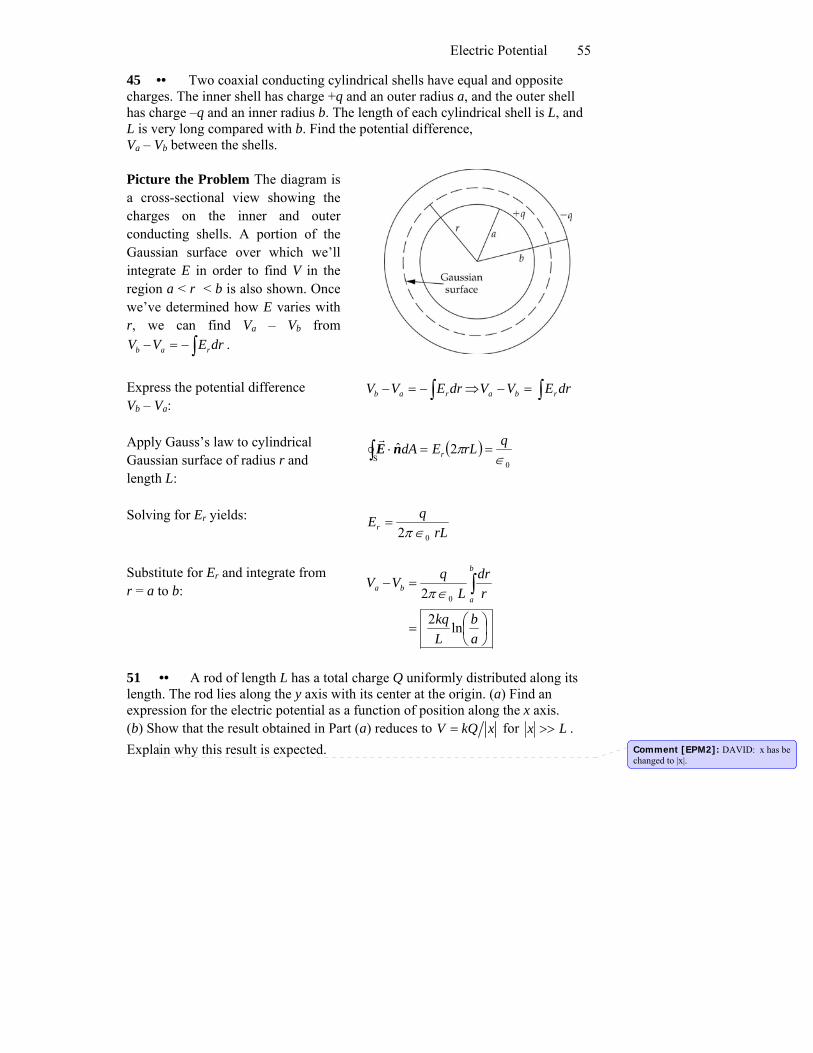
45 •• Two coaxial conducting cylindrical shells have equal and opposite charges. The inner shell has charge +q and an outer radius a, and the outer shell has charge –q and an inner radius b. The length of each cylindrical shell is L, and L is very long compared with b. Find the potential difference, Va – Vb between the shells. Picture the Problem The diagram is a cross-sectional view showing the charges on the inner and outer conducting shells. A portion of the Gaussian surface over which we’ll integrate E in order to find V in the region a < r < b is also shown. Once we’ve determined how E varies with r, we can find Va – Vb from

.

∫ ∫Express the potential difference Vb – Va:

−=− drEVV rab ⇒ =− drEV rbaV

Apply Gauss’s law to cylindrical Gaussian surface of radius r and length L:

( )0

SˆdA⋅∫ nE 2

∈π qrLEr ==

r

Solving for Er yields: rL

q0∈

Er 2π=

Substitute for Er and integrate from r = a to b:

⎟⎞

⎜⎛=

=− ∫bkq

rdr

LqVV

b

aba

ln2

2 0∈π

⎠⎝ aL

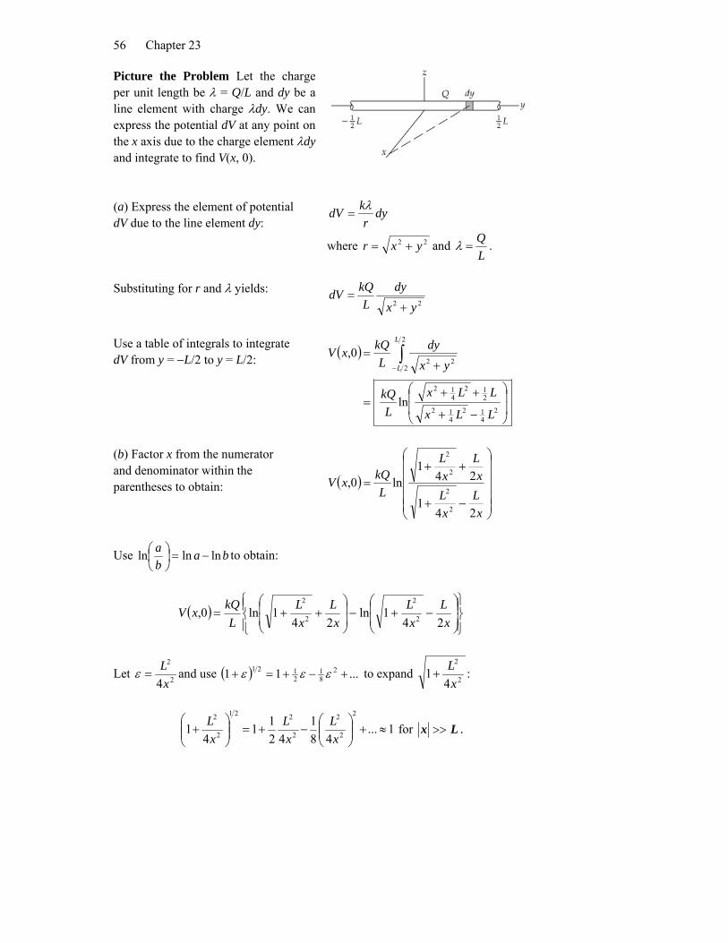
51 •• A rod of length L has a total charge Q uniformly distributed along its length. The rod lies along the y axis with its center at the origin. (a) Find an expression for the electric potential as a function of position along the x axis. (b) Show that the result obtained in Part (a) reduces to V k for Q x= Lx >> . Explain why this result is expected. Comment [EPM2]: DAVID: x has be

changed to |x|.

Chapter 23

56

Picture the Problem Let the charge per unit length be λ = Q/L and dy be a line element with charge λdy. We can express the potential dV at any point on the x axis due to the charge element λdy and integrate to find V(x, 0). (a) Express the element of potential dV due to the line element dy:

dyr

kdV λ=

where 22 yx +=r and LQ

=λ .

Substituting for r and λ yields: 22 yx

dyL

kQdV+

=

( )

Use a table of integrals to integrate dV from y = −L/2 to y = L/2:

⎟⎟

⎠

⎞

⎜⎜

⎝

⎛

−+

++2

412

412

212

412

lnLLx

LLxL

kQ=

+= ∫

−

2

222

0,yx

dyL

kQxVL

L

( )

(b) Factor x from the numerator and denominator within the parentheses to obtain: ⎟

⎠⎜⎝

−+xx 24

1 2⎟⎟⎟⎟⎞

⎜⎜⎜⎜⎛

++=

LLx

Lx

L

LkQxV 24

1ln0,

2

2

2

Use baba lnln −=⎟

⎠⎞

⎜⎝⎛ln to obtain:

( )⎪⎭

⎪⎬⎫

⎟⎟⎠

⎞⎜⎜⎝

⎛−+−⎪⎧

⎟⎟⎠

⎞⎛++

xL

xL

xL

xLkQ

241ln

241 2

2

2

2

⎪⎩⎨ ⎜

⎜⎝

=L

xV ln0,

Let 2

2

41

xL

+2

2

4xL

=ε and use ( ) ...11 281

2121 +−+=+ εεε to expand :

1...11112

2

2

2

221

2

2

≈+⎟⎟⎠

⎞⎜⎜⎝

⎛−+=⎟⎟

⎠

⎞⎜⎜⎛

+x

Lx

Lx

L . 48424⎝

for Lx >>

Electric Potential

57

Substitute for 21

1⎝

⎛+

xL

2

2

4 ⎟⎟⎠

⎞⎜⎜ to obtain:

( )⎭⎬⎟

⎠⎜⎝

−−⎩⎨ ⎟

⎠⎜⎝

+=xxL 2

1ln2

1ln0 ⎫⎞⎛⎧ ⎞⎛ LLkQxV ,

Let x

L=δ ( )

2and use ...1 21 +−=+ δδδln to expand 2 ⎟

⎞⎜⎝⎛ ±

xL2

1ln⎠

:

2

2

4221ln

xL

xL

xL

−≈⎟⎞

⎜⎝⎛ +

⎠ and 2

2

4221

xL

xL

xL

−−≈⎟⎞

⎜⎝⎛ −ln for x >> L.

⎠

Substitute for ⎟⎠⎞

⎜⎝⎛ +

xL2

1ln and ⎟⎠⎞

⎜⎝⎛ −

xL2

1ln and simplify to obtain:

( )x

kQx

Lx

LL

kQxV =⎭⎬⎫

⎟⎟⎠

⎞

⎩⎨⎧

−= 2

2

420,

xL

xL

⎜⎜⎝

⎛−−−2

2

24

Because, for Lx >> , the charge carried by the rod is far enough away from the

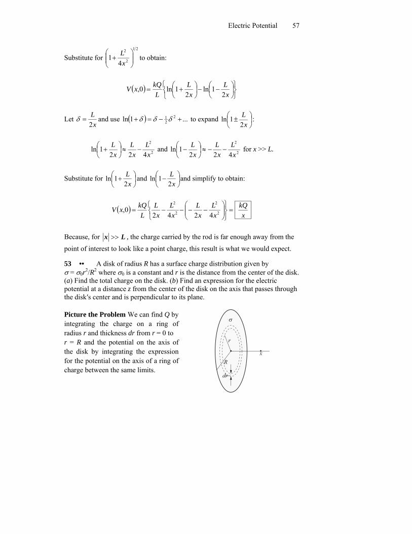
point of interest to look like a point charge, this result is what we would expect. 53 •• A disk of radius R has a surface charge distribution given by σ = σ0r2/R2 where σ0 is a constant and r is the distance from the center of the disk. (a) Find the total charge on the disk. (b) Find an expression for the electric potential at a distance z from the center of the disk on the axis that passes through the disk′s center and is perpendicular to its plane. Picture the Problem We can find Q by integrating the charge on a ring of radius r and thickness dr from r = 0 to r = R and the potential on the axis of the disk by integrating the expression for the potential on the axis of a ring of charge between the same limits.

r

x

R

dr

σ

Chapter 23

58

(a) Express the charge dq on a ring of radius r and thickness dr:

drr

drRrrdrr

32

0

2

2

02

πσ

σπσ ⎟⎟⎠

⎞⎜⎜⎝

⎛=

R

dq

2

2π

=

=

Integrate from r = 0 to r = R to obtain:

21302R

QRπσ

= 020

2 Rdrr πσ=∫

(b)Express the potential on the axis of the disk due to a circular element

of charge drrR

dq 32

02πσ= :

drrkr

kdqdV3

02==

σπrxR 222' +

Integrate from r = 0 to r = R to obtain:

( )[ ]322222

0

022

3

20 22

322 xRxxR

Rk

rxdrr

RkV

R

++−=+

= ∫σπσπ

( )

59 •• A circle of radius a is removed from the center of a uniformly charged thin circular disk of radius b. Show that the potential at a point on the central axis of the disk a distance z from its geometrical center is given by

( )2 2 2 22V z k z b z aπ σ= + − +

( )

,

where σ is the charge density of the disk. Picture the Problem We can find the electrostatic potential of the conducting washer by treating it as two disks with equal but opposite charge densities. The electric potential due to a charged disk of radius R is given by:

⎟⎟⎠

⎞⎜⎜⎝

⎛−+= 112 2

2

xRxkxV σπ

Superimpose the electrostatic potentials of the two disks with opposite charge densities and simplify to obtain:

Electric Potential

59

( )

( )2222

2222

2

22

2

22

2

22

2

22

2

2

2

2

2

2

2

2

2

2

2

2

2

22

2112

11112

112112

axbxk

xax

xbxxk

xax

xbxxk

xax

xbxxk

xa

xbxk

xa

xbxk

xaxk

xbxkx

+−+=

⎟⎟⎠

⎞⎜⎜⎝

⎛ +−

+=⎟

⎟⎠

⎞⎜⎜⎝

⎛ +−

+=

⎟⎟⎠

⎞⎜⎜⎝

⎛ +−

+=⎟

⎟⎠

⎞⎜⎜⎝

⎛+−+=

⎟⎟

⎠

⎞

⎜⎜

⎝

⎛

⎟⎟⎠

⎞⎜⎜⎝

⎛−+−⎟

⎟⎠

⎞⎜⎜⎝

⎛−+=

⎟⎟⎠

⎞⎜⎜⎝

⎛−+−⎟

⎟⎠

⎞⎜⎜⎝

⎛−+=

σπ

σπσπ

σπσπ

σπ

σπσπV

( )

The charge density σ is given by: 22 ab

Q−

=π

σ

( ) ( )

Substituting for σ yields:

( )222222

2 axbxab

kQxV +−+−

=

Equipotential Surfaces

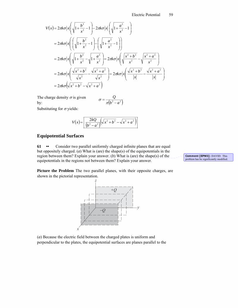
61 •• Consider two parallel uniformly charged infinite planes that are equal but oppositely charged. (a) What is (are) the shape(s) of the equipotentials in the region between them? Explain your answer. (b) What is (are) the shape(s) of the equipotentials in the regions not between them? Explain your answer.

Comment [EPM3]: DAVID: This problem has be significantly modified.

Picture the Problem The two parallel planes, with their opposite charges, are shown in the pictorial representation.

x

z

y

+Q

−Q

(a) Because the electric field between the charged plates is uniform and perpendicular to the plates, the equipotential surfaces are planes parallel to the

Chapter 23

60

( )

charged planes. (b) The regions to either side of the two charged planes are equipotential regions, so any surface in either of these regions is an equipotential surface. 63 •• Suppose the cylinder in the Geiger tube in Problem 62 has an inside diameter of 4.00 cm and the wire has a diameter of 0.500 mm. The cylinder is grounded so its potential is equal to zero. (a) What is the radius of the equipotential surface that has a potential equal to 500 V? Is this surface closer to the wire or to the cylinder? (b) How far apart are the equipotential surfaces that have potentials of 200 and 225 V? (c) Compare your result in Part (b) to the distance between the two surfaces that have potentials of 700 and 725 V respectively. What does this comparison tell you about the electric field strength as a function of the distance from the central wire? Picture the Problem If we let the electric potential of the cylinder be zero, then the surface of the central wire is at +1000 V and we can use Equation 23-23 to find the electric potential at any point between the outer cylinder and the central wire. (a) From Equation 23-23 we have:

⎟⎠⎞

⎜⎝⎛=

rRkrV refln2 λ (1)

where Rref is the radius of the outer cylinder and r is the distance from the center of the central wire and r < Rref.

Solving for 2kλ yields:

( )

⎟⎠⎞

⎜⎝⎛

=

rRrVkrefln

2 λ

At the surface of the wire, V = 1000 V and r = 0.250 mm. Hence:

V 2.ln

2 =λk

( )

228

mm 250.0cm 00.2V 1000

=⎟⎠⎞

⎜⎝⎛

and

( ) ⎟⎠⎞

⎜⎝⎛

rcm 00.2lnV 2.228=rV

( )

Setting V = 500 V yields:

⎟⎞

⎜⎛=

cm 00.2lnV 2.228V 500⎠⎝ r

or

191.2cm 00.2ln =⎟⎠⎞

⎜⎝⎛

r⇒ 191.2cm 00.2 e =

r

Electric Potential

61

Solve for r to obtain:

cm 224.0cm 191 =

00.2.2=

er , closer to

the wire.

(b) The separation of the equipotential surfaces that have potential values of 200 and 225 V is:

V 200V 225Δ rrr −= (2)

Solving equation (1) for r yields: ( ) V 2.2282ref cm 00.2

VkV

eeRr−−

== λ

( )

Substitute for the radii in equation (2), simplify, and evaluate Δr to obtain:

( ) ( )

mm 864.0=

cm 00.2cm 00.2cm 00.2Δ V 2.228V 200

V 2.228V 225

V 2.228V 200

V 2.228V 225

−=−=−−−−

eeeer

( )

(c) The distance between the 700 V and the 725 V equipotentials is:

mm 0966.0

cm 00.2Δ V 2.228V 007

V 2.228V 257

=

−=−−

eer

This closer spacing of these two equipotential surfaces was to be expected. Close to the central wire, two equipotential surfaces with the same difference in potential should be closer together to reflect the fact that the electric field strength is greater closer to the wire. Electrostatic Potential Energy 67 •• (a) How much charge is on the surface of an isolated spherical conductor that has a 10.0-cm radius and is charged to 2.00 kV? (b)What is the electrostatic potential energy of this conductor? (Assume the potential is zero far from the sphere.) Picture the Problem The potential of an isolated spherical conductor is given by

rkQV = , where Q is its charge and r its radius, and its electrostatic potential energy by QV2

1=U . We can combine these relationships to find the sphere’s electrostatic potential energy.

Chapter 23

62

(a) The potential of the isolated spherical conductor at its surface is related to its radius:

RkQV = ⇒

kRVQ =

where R is the radius of the spherical conductor.

Substitute numerical values and evaluate Q:

( )( )

nC 22.3nC 25C

mN10988 2

29

=

⋅×

.22

.8

kV 00.2cm 0.10

=

=Q

(b) Express the electrostatic potential energy of the isolated spherical conductor as a function of its charge Q and potential V:

QVU 21=

Substitute numerical values and evaluate U:

( )( ) J3.22kV 00.2nC 25.2221 μ==U

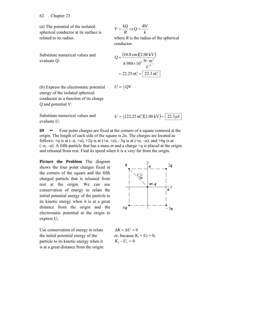
69 •• Four point charges are fixed at the corners of a square centered at the origin. The length of each side of the square is 2a. The charges are located as follows: +q is at (–a, +a), +2q is at (+a, +a), –3q is at (+a, –a), and +6q is at (–a, –a). A fifth particle that has a mass m and a charge +q is placed at the origin and released from rest. Find its speed when it is a very far from the origin. Picture the Problem The diagram shows the four point charges fixed at the corners of the square and the fifth charged particle that is released from rest at the origin. We can use conservation of energy to relate the initial potential energy of the particle to its kinetic energy when it is at a great distance from the origin and the electrostatic potential at the origin to express Ui.

a

a

a2

x

q3−

qm,

yq q2

q6

Δ + Δ = 0UK

0if

or, because Ki = Uf = 0,

Use conservation of energy to relate the initial potential energy of the particle to its kinetic energy when it is at a great distance from the origin:

− =UK

Electric Potential

63

Express the initial potential energy of the particle to its charge and the electrostatic potential at the origin:

( )0i qVU =

Substitute for Kf and Ui to obtain: ( ) 00 =qV ( )2

21 −mv ⇒

mqVv 02

=

( )

Express the electrostatic potential at the origin:

akq

aaaa

26

2222kqkqkqkqV 6320

=

+−

++=

Substitute for V(0) and simplify to obtain: maa2 ⎠⎝

kqkqmqv 2662

=⎟⎞

⎜⎛

=

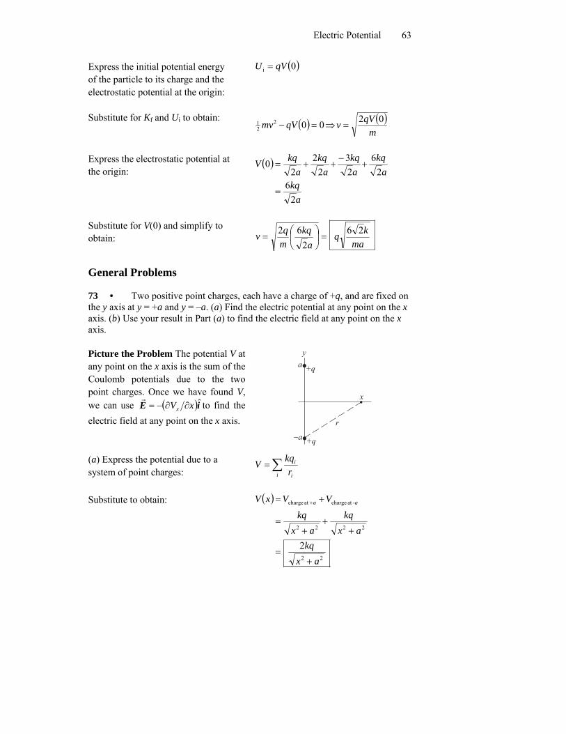
General Problems 73 • Two positive point charges, each have a charge of +q, and are fixed on the y axis at y = +a and y = –a. (a) Find the electric potential at any point on the x axis. (b) Use your result in Part (a) to find the electric field at any point on the x axis. Picture the Problem The potential V at any point on the x axis is the sum of the Coulomb potentials due to the two point charges. Once we have found V, we can use ( )iE ˆxVx ∂∂−=

rto find the

electric field at any point on the x axis.

x

−a+q

a+q

y

r

(a) Express the potential due to a system of point charges: ∑=

i i

i

rkqV

Substitute to obtain: ( )

22 ax +

2222

-at chargeat charge

2kqax

kqax

kq

VVxV aa

=

++

+=

= ++

Chapter 23

64

( )(b) The electric field at any point on the x axis is given by:

( )i

ii

ˆ2

ˆ2ˆ

2322

22

axkqx

axkq

dxd

xVx

+

⎥⎦

⎤⎢⎣

⎡

+−=

∂∂

−E x

=

=r

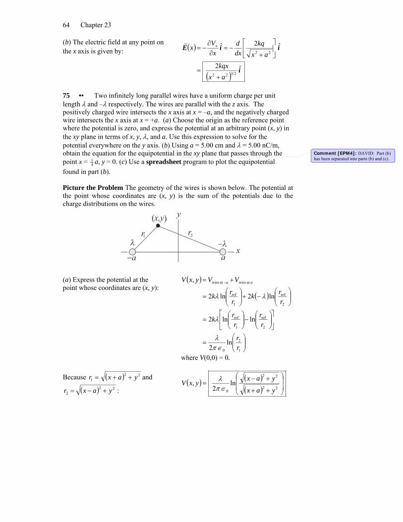
75 •• Two infinitely long parallel wires have a uniform charge per unit length λ and –λ respectively. The wires are parallel with the z axis. The positively charged wire intersects the x axis at x = –a, and the negatively charged wire intersects the x axis at x = +a. (a) Choose the origin as the reference point where the potential is zero, and express the potential at an arbitrary point (x, y) in the xy plane in terms of x, y, λ, and a. Use this expression to solve for the potential everywhere on the y axis. (b) Using a = 5.00 cm and λ = 5.00 nC/m, obtain the equation for the equipotential in the xy plane that passes through the point x = 1

4 a, y = 0. (c) Use a spreadsheet program to plot the equipotential found in part (b).

Comment [EPM4]: DAVID: Part (b) has been separated into parts (b) and (c).

Picture the Problem The geometry of the wires is shown below. The potential at the point whose coordinates are (x, y) is the sum of the potentials due to the charge distributions on the wires.

a−a

λ −λx

y(x,y)

r r1 2

( )(a) Express the potential at the point whose coordinates are (x, y):

= +

( )

⎟⎟⎠

⎞⎜⎜⎝

⎛=

⎥⎦

⎤⎢⎣

⎡⎟⎟⎠

⎞⎜⎜⎝

⎛−⎟⎟

⎠

⎞⎜⎜⎝

⎛=

⎟⎟⎠

⎞⎜⎜⎝

⎛−+⎟⎟

⎠

⎞⎜⎜⎝

⎛=

−

2

ref

1

ref

at wireat wire

ln2ln2

,

rrk

rrk

VVyxV aa

λλ

( )

1

2

0

2

ref

1

ref

ln2

lnln2

rr

rr

rrk

∈πλ

λ

where V(0,0) = 0.

Because ( )221 yaxr ++=

( )and

:222 yaxr +−=

( )( ) ⎟

⎟

⎠

⎞

⎜⎜

⎝

⎛

++

+−=

22

22

0

ln2

,yax

yaxyxV

∈πλ

Electric Potential

65

( )

On the y axis, x = 0 and:

( ) 01ln2

ln2

0

22

22

0

==

⎟⎟

⎠

⎞

⎜⎜

⎝

⎛

+

+=

∈πλ

∈πλ

yaya

,0 yV

(b) Evaluate the potential at ( ) ( ) :0cm,25.10,4

1 =a ( ) ( )( )

⎟⎠⎞

⎜⎝⎛=

⎟⎟

⎠⎜⎜

⎝ +=

53ln

2

ln2

0

241

4

0

∈πλ

∈π aa

⎞⎛ −0,

21

41 λ aa

aV

Equate V(x,y) and ( )0,4

1 aV :

( )( ) 225 y++

22553

x

yx +−=

Solve for y to obtain: 2525.21 2 −−±= xxy

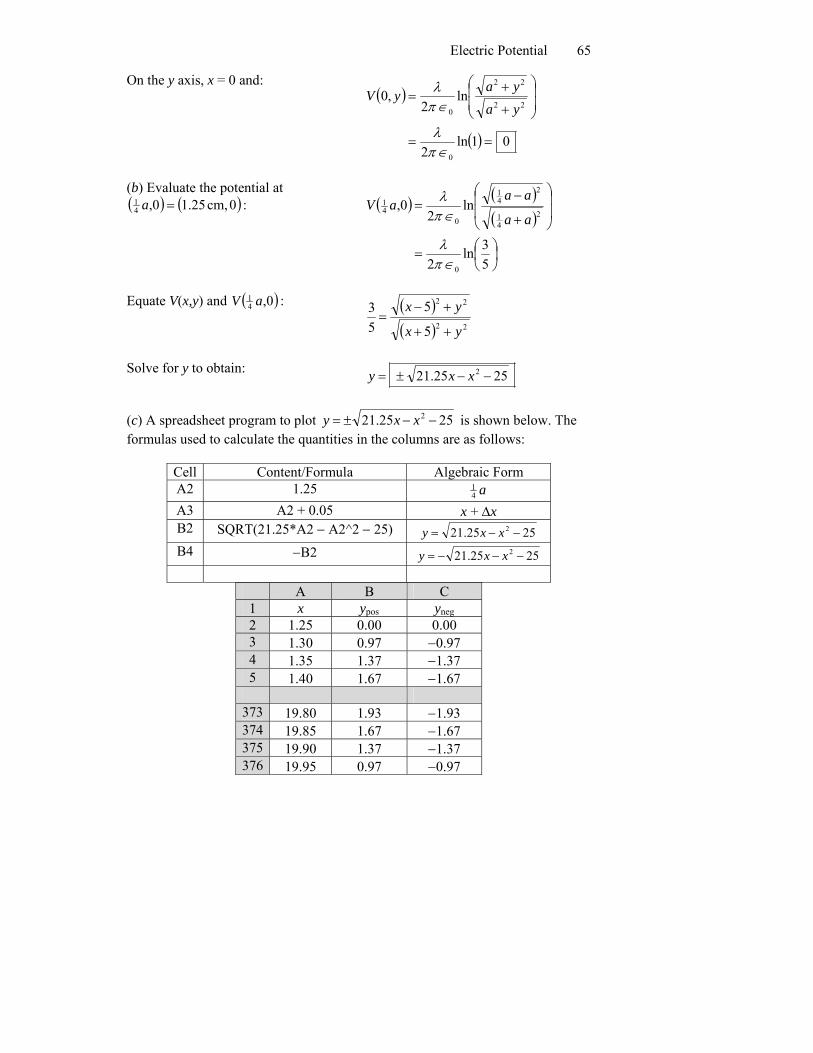
(c) A spreadsheet program to plot 252 −x25.21 −±= xy is shown below. The formulas used to calculate the quantities in the columns are as follows:

Cell Content/Formula Algebraic Form A2 1.25 a4

1 A3 A2 + 0.05 x + Δx B2 SQRT(21.25*A2 − A2^2 − 25) 2525.21 2 −−= xxy B4 −B2 2525.21 2 −−−= xxy

A B C 1 x ypos yneg2 1.25 0.00 0.00 3 1.30 0.97 −0.97 4 1.35 1.37 −1.37 5 1.40 1.67 −1.67

373 19.80 1.93 −1.93 374 19.85 1.67 −1.67 375 19.90 1.37 −1.37 376 19.95 0.97 −0.97

Chapter 23

66

The following graph shows the equipotential curve in the xy plane for

( ) ⎟⎠⎞

⎜⎝⎛=

53ln

20,

041

∈πλaV .

-10

-8

-6

-4

-2

0

2

4

6

8

10

0 5 10 15 20

x (cm)

y (c

m)

87 ••• [SSM] (a) Configuration A consists of two point particles; one particle has a charge of +q and is on the x axis at x = +d and the other particle has a charge of –q and is at x = –d (Figure 23-36a). Assuming the potential is zero at large distances from these charged particles, show that the potential is also zero everywhere on the x = 0 plane. (b) Configuration B consists of a flat metal plate of infinite extent and a point particle located a distance d from the plate (Figure 23-36b). The point particle has a charge equal to +q and the plate is grounded. (Grounding the plate forces its potential to equal zero.) Choose the line perpendicular to the plate and through the point charge as the x axis, and choose the origin at the surface of the plate nearest the particle. (These choices put the particle on the x axis at x = +d.) For configuration B, the electric potential is zero both at all points in the half-space x ≥ 0 that are very far from the particle and at all points on the x = 0 plane—just as was the case for configuration A. A theorem, called the uniqueness theorem, implies that throughout the half-space x ≥ 0 the potential function V—and thus the electric field E

r—for the two configurations

are identical. Using this result, obtain the electric field Er

at every point in the x = 0 plane in configuration B. (The uniqueness theorem tells us that in configuration B the electric field at each point in the x = 0 plane is the same as it is in configuration A.) Use this result to find the surface charge density σ at each point in the conducting plane (in configuration B).

Electric Potential

67

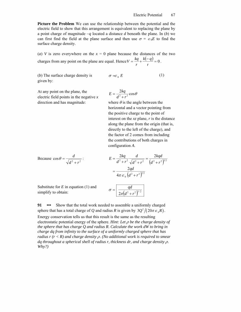
Picture the Problem We can use the relationship between the potential and the electric field to show that this arrangement is equivalent to replacing the plane by a point charge of magnitude −q located a distance d beneath the plane. In (b) we can first find the field at the plane surface and then use σ = ∈0E to find the surface charge density. (a) V is zero everywhere on the x = 0 plane because the distances of the two

charges from any point on the plane are equal. Hence ( )− 0=+=r

qkr

kq

E0

V .

(b) The surface charge density is given by:

σ ∈= (1)

At any point on the plane, the electric field points in the negative x direction and has magnitude:

θcos222 rd

kqE+

=

where θ is the angle between the horizontal and a vector pointing from the positive charge to the point of interest on the xz plane, r is the distance along the plane from the origin (that is, directly to the left of the charge), and the factor of 2 comes from including the contributions of both charges in configuration A.

Because :cos22 rd

d+

=θ

( )

( ) 23220 rd +∈

23222222

42

22

qdrd

kqdrd

drd

kqE

=

+=

++=

π

( )

Substitute for E in equation (1) and simplify to obtain: 2/3222 rd

qd+

=π

σ

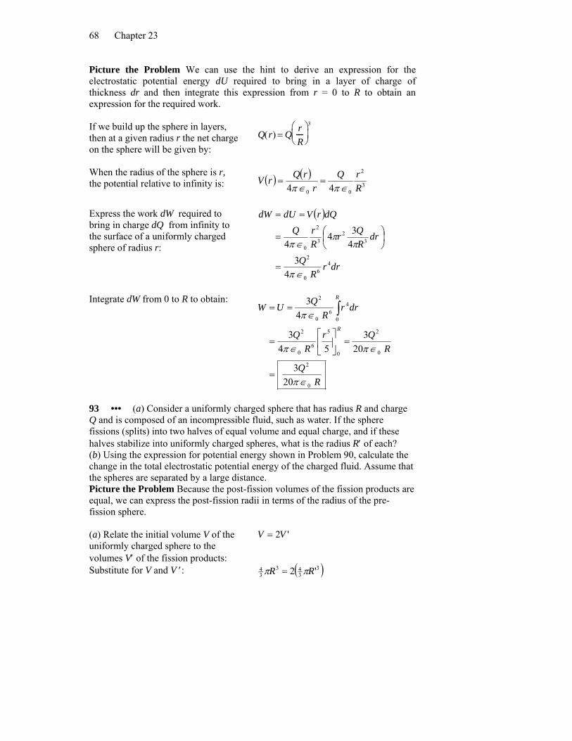
91 ••• Show that the total work needed to assemble a uniformly charged sphere that has a total charge of Q and radius R is given by ( )2

03 20Q Rπ ∈ . Energy conservation tells us that this result is the same as the resulting electrostatic potential energy of the sphere. Hint: Let ρ be the charge density of the sphere that has charge Q and radius R. Calculate the work dW to bring in charge dq from infinity to the surface of a uniformly charged sphere that has radius r (r < R) and charge density ρ. (No additional work is required to smear dq throughout a spherical shell of radius r, thickness dr, and charge density ρ. Why?)

Chapter 23

68

Q(r) = Qr

Picture the Problem We can use the hint to derive an expression for the electrostatic potential energy dU required to bring in a layer of charge of thickness dr and then integrate this expression from r = 0 to R to obtain an expression for the required work. If we build up the sphere in layers, then at a given radius r the net charge on the sphere will be given by:

R⎛ ⎝ ⎜

⎞ 3

( )

⎠ ⎟

When the radius of the sphere is r, the potential relative to infinity is:

( )3

00 44 Rr ∈π∈π

2rQrQrV ==

Express the work dW required to bring in charge dQ from infinity to the surface of a uniformly charged sphere of radius r:

( )

drrR

Q

drR

rR

46

0

2

32

30

3

44

∈π

ππ

∈π⎟⎠

⎜⎝

QrQdQrVdUdW

2

4

34

=

⎞⎛=

==

Integrate dW from 0 to R to obtain:

RQ

RQr

RQ

0

2

0

2

0

5

60

2

3

203

53

∈π

∈π∈=⎥

⎦

⎤⎢⎣

⎡

drrR

QUW

R

R

0

46

0

2

20

4

43

π

∈π

=

=

== ∫

'2VV

93 ••• (a) Consider a uniformly charged sphere that has radius R and charge Q and is composed of an incompressible fluid, such as water. If the sphere fissions (splits) into two halves of equal volume and equal charge, and if these halves stabilize into uniformly charged spheres, what is the radius R′ of each? (b) Using the expression for potential energy shown in Problem 90, calculate the change in the total electrostatic potential energy of the charged fluid. Assume that the spheres are separated by a large distance. Picture the Problem Because the post-fission volumes of the fission products are equal, we can express the post-fission radii in terms of the radius of the pre-fission sphere. (a) Relate the initial volume V of the uniformly charged sphere to the volumes V′ of the fission products:

=

Substitute for V and V ′: ( )3343

34 '2 RR ππ =

Electric Potential

69

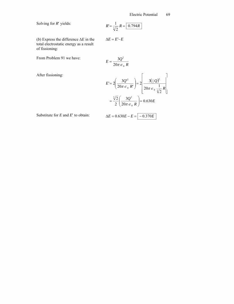
Solving for R′ yields: RR 794.0=R2

1'3

=

(b) Express the difference ΔE in the total electrostatic energy as a result of fissioning:

E E EΔ = −'

From Problem 91 we have: R0∈π

QE2

203

=

After fissioning:

( )

ER

Q

RR

630.020

3

2120

2'20

0

2

30

2

0

=⎟⎟⎠

⎞⎜⎜⎝

⎛

⎥⎥⎥

⎦⎢⎢⎢

⎣

=⎟⎟⎠

∈π

∈π∈πQQE

22

3'32'

3

212

=

⎥⎤

⎢⎡

⎞⎜⎜⎝

⎛=

Substitute for E and E′ to obtain: EEEE 370.0630.0 −=−=Δ

Chapter 23

70