Embed Size (px)
Citation preview
HAL Id: hal-00735721https://hal.archives-ouvertes.fr/hal-00735721
Submitted on 27 Sep 2012
HAL is a multi-disciplinary open accessarchive for the deposit and dissemination of sci-entific research documents, whether they are pub-lished or not. The documents may come fromteaching and research institutions in France orabroad, or from public or private research centers.
L’archive ouverte pluridisciplinaire HAL, estdestinée au dépôt et à la diffusion de documentsscientifiques de niveau recherche, publiés ou non,émanant des établissements d’enseignement et derecherche français ou étrangers, des laboratoirespublics ou privés.
Derivation of soil-specific streaming potential electricalparameters from hydrodynamic characteristics of
partially saturated soilsDamien Jougnot, Niklas Linde, A. Revil, Claude Doussan
To cite this version:Damien Jougnot, Niklas Linde, A. Revil, Claude Doussan. Derivation of soil-specific streamingpotential electrical parameters from hydrodynamic characteristics of partially saturated soils. Va-dose Zone Journal, Soil science society of America - Geological society of America., 2012, 11 (1),pp.10.2136/vzj2011.0086. �10.2136/vzj2011.0086�. �hal-00735721�
1
Derivation of soil-specific streaming potential electrical
parameters from hydrodynamic characteristics of partially
saturated soils
D. Jougnot1, N. Linde
1, A. Revil
2,3, and C. Doussan
4
1 Institute of Geophysics, University of Lausanne, Lausanne, Switzerland;
2 Colorado School of Mines, Green Center, Dept of Geophysics, Golden, CO 80401, USA;
3 ISTerre, CNRS, UMR CNRS 5275, Université de Savoie, 73376 cedex, Le Bourget du Lac,
France
4 EMMAH, UMR 1114, INRA, UAPV, Avignon, France.
Authors contact :
Damien Jougnot: [email protected]
Niklas Linde: [email protected]
André Revil: [email protected]
Claude Doussan: [email protected]
Accepted for publication in Vadose Zone Journal
2
Abstract
Water movement in unsaturated soils gives rise to measurable electrical potential differences
that are related to the flow direction and volumetric fluxes, as well as to the soil properties
themselves. Laboratory and field data suggest that these so-called streaming potentials may be
several orders of magnitudes larger than theoretical predictions that only consider the
influence of the relative permeability and electrical conductivity on the self potential (SP)
data. Recent work has partly improved predictions by considering how the volumetric excess
charge in the pore space scales with the inverse of water saturation. We present a new
theoretical approach that uses the flux-averaged excess charge, not the volumetric excess
charge, to predict streaming potentials. We present relationships for how this effective excess
charge varies with water saturation for typical soil properties using either the water retention
or the relative permeability function. We find large differences between soil types and the
predictions based on the relative permeability function display the best agreement with field
data. The new relationships better explain laboratory data than previous work and allow us to
predict the recorded magnitudes of the streaming potentials following a rainfall event in sandy
loam, whereas previous models predict three orders of magnitude too small values. We
suggest that the strong signals in unsaturated media can be used to gain information about
fluxes (including very small ones related to film flow), but also to constrain the relative
permeability function, the water retention curve, and the relative electrical conductivity
function.
3
1. Introduction
Under unsaturated conditions, water fluxes are typically inferred from state variables
(water content, capillary pressure, or temperature) (e.g. Tarantino et al. 2008, Vereecken et
al., 2008). These local and typically disruptive measurements can be complemented with
geophysical monitoring and subsequent inversion of geophysical data with a larger support-
volume that are sensitive to the above-mentioned state-variables (e.g., Kowalsky et al., 2005).
Most of these techniques infer fluxes by data or model differencing in time or space, that is,
they are not directly measuring the fluxes occurring at the time of the measurements. The self-
potential (SP) method, in which naturally occurring electrical potential differences are
measured, provides data that are directly sensitive to water flow (e.g., Thony et al., 1997). The
origin of this phenomenon is associated with water flow in a charged porous medium, such as
a soil (or more precisely, with the drag of excess charge contained in the diffuse layer in the
pore water that surrounds mineral surfaces). The source current density that creates the SP
signals has several other possible contributors (e.g., related to redox and diffusion processes),
but we focus here on streaming currents, which often tend to dominate in the vadose zone.
The generation and behavior of streaming potentials in porous media under two-phase
flow conditions have been investigated within an increasing number of publications, but
no consensus has been reached concerning how to best model the SP source signals.
Streaming potential responses has been studied at different scales and with different
degrees of control (from the field to the laboratory). Thony et al. (1997) were the first to
demonstrate experimentally a strong linear relationship between SP signals and water flux in
unsaturated soils. Doussan et al. (2002) found based on long-term monitoring in a lysimeter
that even if strong linear relationships are present during and after individual rainfall events,
no linear relationship can explain data from different soil types and water content conditions.
Perrier and Morat (2000) monitored SP signals at an experimental site for one year and
proposed a means to explain observed daily variations by considering vadose zone processes.
Suski et al. (2006) monitored an infiltration test from a ditch. Using surface-based SP
monitoring data from a periodic pumping test, Maineult et al. (2008) observed a clear
correlation between pumping and SP signal, but with a time-varying phase lag between the
measured SP signals at the ground surface and the in situ pressure heads. This phase lag was
explained by Revil et al. (2008) using an hysteretic flow model in the vadose zone. Recently,
Linde et al. (2011) showed that SP sources in the vadose zone might strongly influence the
4
measured response in surface-based SP surveys, which has important ramifications as such
surveys are often interpreted in terms of groundwater flow patterns only.
Field experiments usually suffer from incomplete knowledge about the variation of
relevant variables and boundary conditions with time. It is therefore often necessary to rely on
well-controlled laboratory experiments when deriving equations governing streaming
potentials under unsaturated conditions. Guichet et al. (2003), Revil and Cerepi (2004), Linde
et al. (2007), Revil et al. (2007), Allègre et al. (2010), and Vinogradov and Jackson (2011)
have all investigated streaming potentials in the laboratory using either soil or rock samples or
1D column experiments. In addition to low-frequency signals associated with water flow,
Haas and Revil (2009) demonstrated the existence of bursts in the electrical field associated
with Haines jumps during drainage and imbibition experiments. At an intermediate scale
between laboratory and field conditions, Doussan et al. (2002) conducted a six month
monitoring experiment of SP signals, pressure, and temperature in a lysimeter under natural
conditions (evaporation and rainfall recharge). These authors developed empirical
relationships to relate SP measurements and water flux for different rainfall events, but no
general relationship was found that could explain all the data.
Different approaches have been invoked to explain and model SP signal generation
under unsaturated conditions. Wurmstich and Morgan (1994) proposed an enhancement factor
to the saturated streaming potential coupling coefficient equation to model the SP responses
to a pumping tests of an oil reservoir. Darnet and Marquis (2004) and Sailhac et al. (2004)
introduced Archie’s second law in the traditional Helmholtz-Smoluchowki definition of the
streaming potential coupling coefficient to account for the partial water saturation, but
ignored saturation-induced variations in the relative permeability and excess charge. This
theory, like the one proposed by Wurmstich and Morgan (1994), predict an increase of the
streaming potential coupling coefficient with decreasing water content, which is in
contradiction with laboratory data that generally show decreases with a decreasing water
content (among others, Guichet et al., 2003; Revil and Cerepi, 2004; Vinogradov and
Jackson, 2011). Revil and Cerepi (2004) explained this behavior in terms of the increased
relative importance of surface-related conduction mechanisms with a decreasing water
saturation. Saunders et al. (2006) used the model of Revil and Cerepi (2004) to simulate
streaming potentials during hydrocarbon recovery. Perrier and Morat (2000) suggested that
the streaming potential coupling coefficient should scale with water saturation according to
the ratio of relative permeability and relative electrical conductivity. Linde et al. (2007) and
Revil et al. (2007) extended this model by suggesting that also the excess charge need to be

5
considered and they scaled it with the inverse of the water saturation. This scaling based on
volume averaging is simplified as the volume averaged values are typically very different
from the flux-averaged excess charge that influence measured streaming potentials (Linde et
al., 2009). Recently, Jackson (2008; 2010) and Linde (2009) proposed models based on a
capillary bundle that account for the pore size distribution of partially saturated porous media
in the prediction of streaming potentials. The resulting predictions are strongly influenced by
both the pore size distribution and the electrical double layer, but no attempts has been made
to date to relate these models to available soil-specific hydrodynamic properties. The aim of
the present contribution is to propose and test two different models based on soil
hydrodynamic properties.
We use the pore size distribution and the excess charge distribution in the Gouy-
Chapman layer to derive the effective flux-averaged excess charge density dragged in the
medium. The model for each soil type is derived from soil-specific hydrodynamic functions,
namely the water retention and the relative permeability functions. For each of these
functions, we evaluate for a range of soil textural classes how the effective excess charge in
the pore water varies with the effective water saturation. The resulting relationships are then
used to determine how the streaming potential coupling coefficient is expected to vary with
the effective water saturation. The two approaches are evaluated against the laboratory data of
Revil and Cerepi (2004) and the lysimeter monitoring data of Doussan et al. (2002).
2 Soil hydrodynamic function-based models
2.1 Governing equations and previous work
The two equations that describe the SP response of a given source current density js (A
m-2
) is given by Sill (1983)
j E jS, [1]
j 0, [2]
where j (A m-2
) is the total current density,
(S m-1
) is the bulk electrical conductivity,
E (V m-1
) is the electrical field, and
(V) is the electrical potential. The source
current densities can be understood as forcing terms that perturb the geological system from
electrical neutrality. This induces an electrical current that re-establishes electrical neutrality
and the SP response are the associated voltage differences created by this current. In the
6
absence of external source currents it is possible to combine these equations to yield the
following governing equation
jS. [3]
This partial differential equation can be solved using finite-element or finite-difference
techniques given appropriate boundary conditions and exhaustive knowledge about the spatial
distribution of and the source current density js (e.g., Sill, 1983). In the field, the electrical
conductivity distribution can be estimated using electrical resistivity tomography (e.g.,
Günther et al., 2006) or electromagnetic methods (e.g., Everett and Meju, 2005), while the
influence of the uncertainty in these models can be evaluated through sensitivity tests (e.g.,
Minsley, 2007). The focus of this paper is on how to predict js from soil-specific
hydrodynamic functions.
Three sources of js may dominate in natural media: electrokinetic processes that are
directly related to the water flux in the medium (related to the streaming current density jS
EK ),
redox processes, and electro-diffusion (see, among others Revil and Linde, 2006). Redox
processes can create large SP signals but only under certain restrictive conditions (see
discussion in Revil et al., 2009). In the present study, we restrict ourselves to electrokinetic
processes that typically dominate in hydrological applications. The water flux follows
Darcy’s law and can be described by the Darcy velocity
u (m s-1
) defined by
u k
w
pw
wgz K
wH , [4]
where k (m2) is the permeability, w (1.002 10
-3 Pa s at T = 20 °C) is the dynamic viscosity,
pw (Pa) is the water pressure, w
is the water density (1000 kg m-3
), g is the gravitational
acceleration (9.81 m s-2
), Kw
(m s-1
) is the hydraulic conductivity, and H (m) is the hydraulic
head (m). In saturated media, the Darcy velocity is related to the pore water velocity v (m s-1
)
and the porosity (-) by u v .
The streaming current density ( jS
EK ) is typically described using the streaming
potential coupling coefficient
CEK
(V m-1
)
jS
EK C
EKH , [5]
with
CEK
defined as
CEK
Hj 0
. [6]
7
For water-saturated conditions (denoted by superscript sat), Revil and Leroy (2004) relate
CEK
sat to the excess charge in the electrical double layer as
CEK
satQ
v
sat
k
satw
, [7]
where Qv
sat
1 fQ Q v
is the excess charge in the Gouy-Chapman layer per pore water
volume with fQ the fraction of excess charge in the Stern layer and Qv (C m
-3) the total excess
charge that counter balance the mineral surface charges. Equation [7] can be extended for
partial saturation in a water-wet media for which we explicitly indicate a dependence of the
material properties on the water saturation Sw
CEK
(Sw
) Qv(S
w)
(Sw
)
Kw
(Sw
)
w
. [8]
Note that several functions describing (Sw
) exist in the literature (among other Waxman and
Smits, 1968; Rhoades et al., 1989). Laloy et al. (2011) recently published a study
investigating the most appropriate pedo-electrical model for a loamy soil.
It is also possible to express jS
EK at partial saturations as (Revil et al., 2007)
jS
EK Q
v(S
w)u. [9]
As a first approximation, Linde et al. (2007) and Revil et al. (2007) proposed that
Qv(S
w) scales with the inverse of Sw, that is,
Qv(S
w)
Qv
sat
Sw
. [10]
Linde (2009) shows that the effective excess charge Qv
eff(S
w) dragged in the pore space must
be considered as a flux-averaged property that depends on the pore space geometry and the
water phase (see also Jackson, 2010). Equation [10] that is based on volume-averaging is
therefore only a valid expression for predicting SP signals when Qv(S
w) is evenly distributed
throughout the pore space.
In soil hydrology, soil hydrodynamic properties are described by the water retention
and the relative permeability function. The first function describes the relationship between
the water content, w
(-), (or saturation, Sw
(-)) and the matric potential, h (m), whereas the
second relates the hydraulic conductivity to the water content. Theoretical formulations of
these hydrodynamic properties have often been derived by conceptualizing the soil as a
8
bundle of cylindrical capillaries with a given size density distribution, tortuosity, and
connectivity (e.g. Jury et al., 1991).
In the following section 2.2, we describe the electrokinetic behavior and the electrical
conductivity of a given capillary. Then in section 2.3 and 2.4 we present two approaches to
determine Qv
eff(S
w) by defining the pore space as a bundle of capillaries that is derived either
from the water retention function (i.e., the WR approach) or the relative permeability function
(i.e., the RP approach).
2.2 Effective excess charge in a capillary
We consider a capillary with a radius R and a length Lc. We let r be the distance from
the pore wall (r = 0) to the center of the capillary (
r R ). The capillary is saturated by an
electrolyte of N ionic species i, with concentration ci
0
(mol m-3
), valence zi (-), and charge
qi ez
i (C), where e (1.6 10
-19 C) is the elementary charge. The ionic strength I (mol m
-3) of
the electrolyte is
I 1
2zi
2ci
0.
i 1
N
[11]
Note that the ionic strength is equal to the salinity for binary symmetric 1:1 electrolyte (e.g.,
NaCl).
We assume—as for silicate and aluminosilicate minerals—that the pore walls have a
negative surface charge (the case of positive surface charge can be treated in an analogous
manner). To assure electrical neutrality, there exists a balancing excess of cations in the pore
water (counterions, while anions are called co-ions). Most of the excess charge is located
close to the pore wall in the fixed Stern layer and the remaining part is distributed in the
diffuse Gouy-Chapman layer, while the free electrolyte is defined by the absence of excess
charge (e.g., Leroy and Revil, 2004). Figure 1a presents a sketch of the charge distribution in
the different layers.
The Stern layer contains only counterions (with or without their hydration shell) and
its thickness is negligible for typical soils. For example, molecular dynamics simulations in a
0.1 M NaCl–montmorillonite system shows that the thickness of the Stern layer is about 6.1 Å
(Tournassat et al., 2009). The interface between the Stern layer and the Gouy-Chapman layer
is assumed to correspond to the shear plane, which separates the stationary fluid (due to
surface effects) and the moving fluid (see among others, Hunter, 1981; Revil et al., 2002).
9
The electrical potential along this plane is commonly assumed to correspond to the zeta
potential
(V). This potential depends for a given mineral, among other things, on ionic
strength, temperature, and pH (e.g., Revil et al., 1999).
The thickness of the Gouy-Chapman layer corresponds roughly to two Debye lengths
lD(Hunter, 1981) defined by
lD
kBT
2 Ie2
, [12]
where r
0 (F m
-1) is the pore water permittivity, kB (1.381 10
-23 J K
-1) is the
Boltzmann constant, T (K) is the absolute temperature,
0 = 8.854 10
-12 F m
-1 is the
permittivity of vacuum and r=80.1 at T=20C is the relative permittivity of water. The Gouy-
Chapman layer contains distributions of both anions and cations that are linked to the local
electrical potential in the pore water f (r ) . Pride (1994) expressed for the thin double
layer assumption (i.e., the thickness of the double layer is small compared to the pore size)
how the local electrical potential depends on the
-potential and the distance r from the shear
plane as (see also Fig. 2a)
(r ) exp( r / lD
) . [13]
This equation neglects the effects of the charges of the opposite capillary wall (for the case of
overlapping Gouy-Chapman layers, see Gonçalvès et al., 2007), which is a valid assumption
in most soils under typical conditions. The counterion and co-ion distributions ci f (r ) in
the pore-water follow (see Fig. 2b)
ci(r ) c
i
0exp
qi
kBT
, [14]
where ci
0 is the ionic concentration of i far from the mineral surface (i.e., in the free
electrolyte). The excess charge distribution Qv(r ) (C m
-3) in the capillary is (excluding the
Stern layer) given by (see Fig. 1b)
Qv(r ) N
Aqici(r )
i 1
N
, [15]
with NA = 6.022 1023
mol-1
being Avogadro’s number.
For a laminar flow rate, the velocity distribution v(r) in a capillary of radius R with a
given hydraulic head vertical gradient dh dz is approximated by the Poiseuille model (Fig.
1c)
10
v(r ) wg
4wR
2 (R r )
2 dh
dz, [16]
where is the tortuosity of the capillary (Lc/L), where L is the length over which the pressure
difference is applied. The average velocity vR (m s
-1) in the capillary is
vR
wg
8wR
2 dh
dz. [17]
By integration of the flux over the total area of the capillary, one can recover the flux-
averaged excess charge, that is, the effective excess charge carried by the water flux in the
capillary Qv
eff ,R (C m-3
) by
Qv
eff , R
Qv
(r )v(r )r dr
r 0
R
v(r )r dr
r 0
R
. [18]
Figure 1 presents a conceptual view of the electrical double layer model (Fig. 1a), the
calculated excess charge distribution using Eq. [15] (Fig. 1b), and the calculated pore fluid
velocity using Eq. [16] (Fig. 1c).
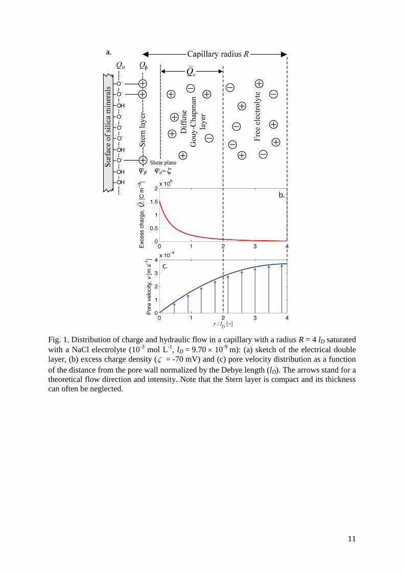
11
Fig. 1. Distribution of charge and hydraulic flow in a capillary with a radius R = 4 lD saturated
with a NaCl electrolyte (10-3
mol L-1
, lD = 9.70 10-9
m): (a) sketch of the electrical double
layer, (b) excess charge density ( = -70 mV) and (c) pore velocity distribution as a function
of the distance from the pore wall normalized by the Debye length (lD). The arrows stand for a
theoretical flow direction and intensity. Note that the Stern layer is compact and its thickness
can often be neglected.
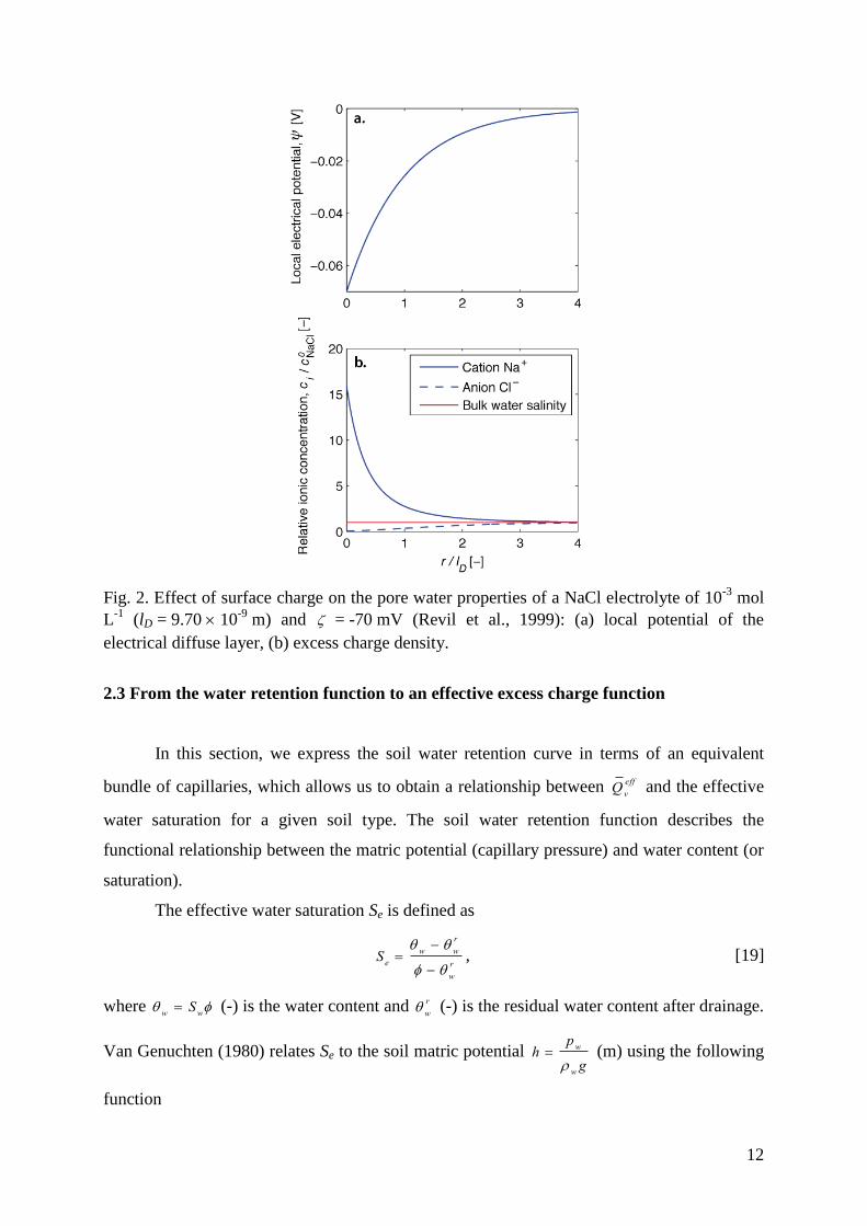
12
Fig. 2. Effect of surface charge on the pore water properties of a NaCl electrolyte of 10-3
mol
L-1
(lD = 9.70 10-9
m) and = -70 mV (Revil et al., 1999): (a) local potential of the
electrical diffuse layer, (b) excess charge density.
2.3 From the water retention function to an effective excess charge function
In this section, we express the soil water retention curve in terms of an equivalent
bundle of capillaries, which allows us to obtain a relationship between Qv
eff and the effective
water saturation for a given soil type. The soil water retention function describes the
functional relationship between the matric potential (capillary pressure) and water content (or
saturation).
The effective water saturation Se is defined as
Sew
w
r
w
r, [19]
where w S
w (-) is the water content and
w
r (-) is the residual water content after drainage.
Van Genuchten (1980) relates Se to the soil matric potential h pw
wg
(m) using the following
function
13
Se 1
VGh
nVG
mVG
, [20]
where
VG
(m-1
) corresponds to the inverse of the air entry matric potential, while
nVG
and
mVG
1 1
nVG
are curve shape parameters. The air entry matric potential corresponds to the
matric potential (he) at which the soil starts to desaturate.
Another popular water retention function is the one of Brooks and Corey (1964)
Se
he
h
BC
for
h he, [21]
Se 1 for
h he, [22]
with he the air entry pressure (m) and
BC
a parameter related to the pore size distribution.
By considering the soil as a bundle of capillaries and applying the Young-Laplace
equation, it is possible to relate an equivalent radius Rj (m) to the capillaries j that drain at a
specific matric potential by
h 2 cos
wgR
j
, [23]
where
(0.0727 N m-1
at T=20°C) is the surface tension of water,
is the contact angle
(often considered to be 0°, which yields cos
= 1, see Bear, 1972).
Using Eq. [20 or 21] and Eq. [23] it is thus possible to relate, for a given Se, the size of
the capillaries
RSe
that drain at an incremental change in Se. This allows us to determine the
range and capillary densities of a bundle corresponding to a soil with a given water retention
curve. We define the capillary size distribution fWR
R as
fWR
R dR SeRSe
Rm in
RSe
. [24]
At the scale of the capillary bundle, the electrical formation factor can be expressed
under saturated conditions, as
1
F lim
S 0
w
m, [25]
where S
is the surface conductivity and w
is the electrical conductivity of the pore water,
respectively, and m is the cementation index defined by Archie (1942). This exponent is
inversely related to the connectivity of the pore space. We assume that the electrical tortuosity
under saturated conditions =F1-m also describes the hydrological tortuosity (e.g., Lesmes
and Friedman, 2005).
14
The normalized volumetric flux of water in the pore
v (Se) (m
3 s
-1 m
-2 = m s
-1) of the
soil can be computed as the sum of the flux of all capillaries up to the size RSe
v(Se)
vR
(R ) fWR
(R )
Rm in
RSe
dR
fWR
(R )
Rm in
RSe
dR
. [26]
This approach (WR) to calculate Qv
eff(S
e) is based on flux-averaging all charges carried by all
the capillaries as determined from the water retention curve. We thus define the effective
excess charge Qv
eff(S
e) as
Qv
eff(S
e)
Qv
eff , RvR
(R ) fWR
(R )
Rm in
RSe
dR
vR
(R ) fWR
(R )
Rm in
RSe
dR
. [27]
It is then possible to obtain CEK
(Sw
) by introducing the appropriate (Sw
) function, Eqs. [26]
and [27] in Eq. [8]. Note that any hysteretic properties of primarily the water retention
function (e.g. Mualem, 1984) but also (Sw
) (Knight, 1991) make the Qv
eff(S
e) function
hysteretic.
2.4 From the relative permeability function to the effective excess charge
In this section, we present an alternative formulation to calculate Qv
eff(S
e) that we term
the RP approach in which we use the relative permeability function. In this approach, we
obtain an equivalent capillary distribution corresponding to a soil with a given relative
permeability function that is then used to determine the Qv
eff(S
e) relationship.
The relative permeability kw
rel(S
e) is defined as
kw
rel(S
e)
Kw
(Se)
Kw
sat, [28]
where Kw
(Se) and K
w
sat , are the partially saturated and the fully saturated hydraulic
conductivity (m s-1
), respectively.
Mualem (1976) proposes the following relationship to determine the relative hydraulic
conductivity from the soil water retention curve
15
kw
relSe S e
dSe
h0
Se
dSe
h0
1
2
, [29]
where is a dimensionless parameter that accounts for hydraulic tortuosity and correlation
between pores as a function of Se (a typical choice is = 0.5). Van Genuchten (1980)
introduced his soil water retention function (Eq. [20]) into Mualem’s model (Eq. [29])
resulting in the widely used van Genuchten-Mualem (VGM) model
kw
relSe S e
1 1 S
e
1 mVG mVG
2
. [30]
Another popular relative permeability function is the one of Brooks and Corey (1964)
that uses a power-law function based on their
BC
(Eq. [21]) parameter
kw
relSe S e
2
BC
3
. [31]
We now derive a capillary size distribution fRPR similarly as for f
WRR in Eq.
[24]. Instead of using the water retention function and Eq. [23], we now use Eq. [17] together
with the derivative of the relative permeability function [Eq. 30 or 31] to derive the equivalent
RSeSe that drains at a given Se as
RSe
2Se
8w
wg
Kw
sat
w
r
kw
relSe
Se
. [32]
After having determined fRPR from S
eRSe , we replace f
WRR in Eq. [27] to determine
the Qv
eff(S
e) relationship. One can then recover C
EK(S
w) by inserting the resulting Q
v
eff(S
e)
relationship, an appropriate (Sw
) function, and Eq. [32] into Eq. [8].
3. Results
3.1 Prediction of the relative excess charge and coupling coefficient for a soil data set
We first derive the Qv
eff(S
e) relationships of our two approaches using a database of
hydrodynamic soil-specific functions (Carsel and Parrish, 1988) compiled from soil water
retention measurements of more than 5000 soil samples that are grouped into 12 textural
categories. We use the average values of the Van Genuchten parameter ( ,w
r ,
VG
, and
nVG
)
16
and the saturated hydraulic conductivity ( Kw
sat ) for each textural category (see Table 1) to
calculate the expected Qv
eff(S
e) function using the WR (section 2.3) and RP approach (section
2.4).
We hereafter consider the soils presented in Table 1 as being saturated by a NaCl
electrolyte at T = 20°C with an ionic strength of I = 5 10-3
mol L-1
. From the empirical
relationship proposed by Worthington et al. (1990), this salinity yields a water conductivity
equal to w
= 0.0603 S m-1
. Considering this electrolyte and its concentration, a typical zeta
potential at the surface of silica minerals is
= -61.1 mV (Revil et al., 1999). We consider
hereafter that all the capillary surfaces have this zeta potential.
Table 1. Average values of the Van Genuchten water retention and relative permeability
model parameters and saturated hydraulic conductivity of textural soil types (from Carsel and
Parrish, 1988).
Texture a.
[-] w
r [-]
VG
[m-1
]
nVG
[-] Kw
sat [m s-1
] Number of
samples b.
Clay 0.38 0.068 0.8 1.09 5.56 10-7
333
Clay loam 0.41 0.095 1.9 1.31 7.22 10-7
360
Loam 0.43 0.078 3.6 1.56 2.89 10-6
735
Loamy sand 0.41 0.057 12.4 2.28 4.05 10-5
315
Silt 0.46 0.034 1.6 1.37 6.94 10-7
83
Silt loam 0.45 0.067 2.0 1.41 1.25 10-6
1093
Silty clay 0.36 0.070 0.5 1.09 5.56 10-8
274
Silty clay loam 0.43 0.089 1.0 1.23 1.94 10-7
631
Sand 0.43 0.045 14.5 2.68 8.25 10-5
246
Sandy clay 0.38 0.100 2.7 1.23 3.33 10-7
46
Sandy clay loam 0.43 0.089 1.0 1.23 3.64 10-6
214
Sandy loam 0.41 0.065 7.5 1.89 1.23 10-5
1183
a. The textural groups correspond to the USDA classification scheme
b. Average number of samples used to determine the parameters for each soil texture
Figure 3 presents the evolution of the relative excess charge Qv
eff , rel (i.e., normalized
by the value at full saturation) using the hydrodynamic properties of the various textural
classes (Table 1) and the two proposed approaches. Both models predict an important increase

17
of Qv
eff , rel with decreasing saturation. This is consistent with the assumption of Linde et al.
(2007), but the new models show much stronger increases at low saturations (three to seven
orders of magnitudes depending on the soil type and approach used). The WR approach (Fig.
3a) predicts increases of Qv
eff , rel that are several orders of magnitudes larger than for the RP
approach (Fig. 3b).
Fig. 3. The Qv
eff , rel(S
e) relationships computed by the WR (a.) and RP approaches (b.). The
solid black lines correspond to the model of Linde et al. (2007) (Qv(S
w) Q
v
sat
Sw
) for the
different soil types (the many neighboring lines arise due to differences in the residual water
content among soil types).
Jardani et al. (2007) propose the following empirical relationship between effective
excess charge (Qv
eff , sat ) and permeability k (m2) under saturated conditions
log10
(Qv
eff , sat) 0.82 log
10(k ) 9.23. [33]
Figure 4 displays the predicted Qv
eff , sat as a function of k for the two approaches. For each
approach, the predictions closely follow a log-log relationship. The correspondence with the
general trend of the experimental data is overall satisfactory, but the absolute values are rather
bad for the WR approach (the permeability is over estimated and the Qv
eff , sat is
underestimated). This is due to the simplification made in the WR approach when computing
the permeability directly from the water retention function, while the RP approach use the
permeability of Carsel and Parrish (1988) (calculated from Kw
sat in Table 1). The resulting
linear regression models
log10
(Qv
eff , sat) 0.77 log
10(k ) 9.14 , [34]
18
log10
(Qv
eff , sat) 0.76 log
10(k ) 8.01 , [35]
for the WR and RP approach, respectively, are rather similar to Eq. [33]. Sensitivity tests
based on the ionic strength have shown that when I increases, Qv
eff , sat decreases (within half an
order of magnitude for I 104
;101
mol L-1
), but the slope of the log-log relationship
remains similar to Eq. [34] and [35]. These results indicate a strong relationship between Qv
eff
and k through the pore size distribution.
Fig. 4. The predicted effective excess charge using the WR and RP approaches for the
different soil textures in saturated conditions. The Jardani et al. (2007) empirical relationship
is shown with other data.
Following the proposed approaches, it is possible to predict the evolution of the
streaming potential coupling coefficient from three soil specific parameters [Eq. 8]: w
(h ) ,
Kw
(h ) , and (Sw
) . But, to the best of our knowledge, very few published datasets on soil
samples are available that include all three relations. We use the data from Doussan and Ruy
(2009) that measured these relationships for: Fontainebleau sand, Collias loam, and Avignon
silty clay loam (Fig. 5). As pointed out by the authors, the data cannot be properly described
by the traditional water retention and relative permeability functions. We used a cubic
interpolation function to describe the parameter evolution with respect to matric potential.
19
Due to the significant standard deviation of the hydraulic conductivity data, we used the mean
as proposed by Doussan and Ruy (2009). We extrapolated the relative permeability up to h =
106 m based on the last data points and van Genuchten Mualem parameters for corresponding
soils.
Fig. 5. Properties of three different soil types: (a.) water content and (b.) hydraulic
conductivity as a function of matric potential, and (c.) electrical conductivity as a function of
water content. Symbols correspond to measurements of Doussan and Ruy (2009), while the
dashed lines represent the interpolations of the measurements used in this study.
Figure 6 shows Qv
eff , rel(S
e) and C
EK
rel(S
e) predicted from Eq. [8] using the WR and RP
approaches. Figure 6a and 6b show that the predicted excess charges have a similar behavior
as for the averaged Carsel and Parrish parameters (Fig. 3), with Qv
eff(S
e) varying strongly
between soil types. From the predicted Qv
eff , rel(S
e) , the interpolated K
w(h ) (Fig. 5b), and
(Sw
) (Fig. 5c), we predicted how the streaming potential coupling coefficient varies with
20
saturation (Fig. 6c and 6d). The behavior of CEK
rel(S
e) strongly depends on the different
parameters.
Fig. 6. Relative excess charge (a., b.) and streaming potential coupling coefficient (c., d.) as a
function of Se predicted by the WR and RP approaches, respectively. These predictions have
been calculated from the parameter functions showed in Fig. 5. The thin black lines in Fig. 6a.
and 6b. correspond to the model of Linde et al. (2007) Qv(S
w) Q
v
sat
Sw
.
3.2 Application to laboratory data
We now apply the WR and RP approaches to the laboratory data of Revil and Cerepi
(2004). These data include electrical conductivity, capillary pressure and streaming potential
coupling coefficient as a function of saturation for two dolomite core samples. The NaCl
brine used for the measurements had an ionic strength I = 8.6 10-2
mol L-1
and a
conductivity of w
= 0.93 S m-1
. For the electrical behavior, Revil and Cerepi (2004) use
21
Archie’s second law to model the relative electrical conductivity rel (S
w)
sat S
w
n . The
hydrological behavior is described using the Brooks and Corey model (Eqs. [21], [22], and
[31]). Table 2 presents the parameters used by Revil and Cerepi (2004) to describe the
electrical and hydrological properties of the two samples (Figs. 7a and 7b).
Table 2. Electrical and hydrologic parameter values used for the dolomite samples.
Sample Porosity
[-] a.
Electrical parameter Hydrological parameter
m [-] a. n [-]
a. S
w
r [-] b.
he [m]
b. BC [-]
b.
E3 0.203 1.93 a. 2.70 0.36 2.40 0.87
E39 0.159 2.49 a. 3.48 0.40 11.52 1.65
a. From Revil and Cerepi (2004)
b. Parameters fitted from Revil and Cerepi (2004) experimental results
Figure 7c presents the predicted relative streaming potential coupling coefficients
using the WR and RP approaches and the predictions of Revil et al. (2007) (see Eq. [10]). The
relative streaming potential coupling coefficient predicted from the water retention function
(Fig. 7b) fits the E3 sample measurements very well and provide satisfactory values for the
E39 sample (Fig. 7c). For all samples, the RP approach tends to overestimate the relative
streaming potential coupling coefficient. Note that the relative permeability function is not
based on actual measurements, but was derived from the Brooks and Corey (1964) model that
is based on the assumption that the BC
describing the water retention function is appropriate
to describe the relative permeability function (Eq. [31]). The volume averaging approach of
Linde et al. (2007) (Eq. [10]) clearly underestimates CEK
rel(S
w) (see also discussion in Allègre
et al., 2011). The predicted Qv
effSw from the WR approach is at low saturations several
orders of magnitude larger than the predictions of Linde et al. (2007) (e.g.,
Qv
eff(S
w
r) 3.4 10
5Q
v(S
w
r) ).
22
Fig. 7. Application of the proposed approaches to a data set obtained on two dolomite samples
from Revil and Cerepi (2004): (a) Relative electrical conductivity, (b) matric potential, and
(c) relative streaming potential coupling coefficient versus saturation. The two thin dashed
lines in Fig 6c represents the predicted values for the approximation Qv(S
w) Q
v
sat
Sw
.
3.3 Application to a lysimeter experiment
We now apply our model to the experimental data acquired by Doussan et al. (2002)
in a lysimeter with a 9 m2 surface and a 2 m height located at the INRA experimental field
site in Avignon, France. The lysimeter was filled with a local sandy loam and instrumented to
monitor unsaturated vertical hydraulic flux. The matric potential was monitored at two depths
(30 and 40 cm below ground surface) using two tensiometers for a period of 6 months, while
SP data were acquired—at two different locations—between the same two depth intervals
using unpolarizable Pb/PbCl2 electrodes (Petiau, 2000) at a 20 cm distance from the
tensiometers. The electrodes located at 30 cm depth were chosen as references. The SP data
were corrected for temperature effects following Petiau (2000). The pore water conductivity
23
was measured punctually using suction cups at a depth of 35 cm. The soil cation exchange
capacity (CEC) of the soil was measured under laboratory conditions using the Metson
method (Metson, 1956).
The water retention curve and the relative permeability function of the sandy loam
were determined under laboratory conditions using the Wind evaporation method (Tamari et
al., 1993). The two hydrodynamic functions could not be adequately fitted using the same van
Genuchten parameters (see Table 3 for the individually best fitting van Genuchten
parameters).
Table 3. Soil properties of the sandy loam soil of Doussan et al. (2002).
[-] w
r [-]
VG
[m-1
]
nVG
[-] Kw
sat [m s-1
]
Water retention function 0.44 0 1.13 1.36 -
Relative permeability function 0.44 0 0.28 1.33 1.25 10-7
The electrical behavior of the soil was modeled using the Waxman and Smits (1968)
model
Sw
n
FwS
Sw
, [36]
with parameter values F = 4.54, n = 1.877 (the saturation index) and S
= 0.109 S m-1
. Due
to rainwater infiltration and evaporation, the water conductivity was changing with time as
inferred from the measurements in the suction cups (w 0.06; 0.20 S m
-1).
We now test our proposed approaches on rainfall events occurring during the
monitoring period. The climatic conditions during the 6 months can be divided into two parts.
No major rain event occurred during the first 90 days. Then a series of rainfall events
occurred and we chose the five major events at days 91, 100, 107, 119, and 131. Following
Doussan et al. (2002), we divide the rainfall events into an infiltration and a drainage phase.
The infiltration phase correspond to an increase of the flux as the rainwater reaches the
sensors, while the drainage part is characterized by the decrease of both water content and
flux. In their interpretation, Doussan et al. (2002) established different relations between the
SP signal and the water flux between these two phases.
24
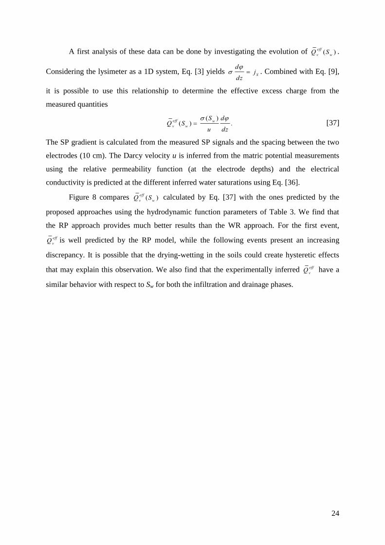
A first analysis of these data can be done by investigating the evolution of Qv
eff(S
w) .
Considering the lysimeter as a 1D system, Eq. [3] yields d
dz j
S. Combined with Eq. [9],
it is possible to use this relationship to determine the effective excess charge from the
measured quantities
Qv
eff(S
w)
(Sw
)
u
d
dz. [37]
The SP gradient is calculated from the measured SP signals and the spacing between the two
electrodes (10 cm). The Darcy velocity u is inferred from the matric potential measurements
using the relative permeability function (at the electrode depths) and the electrical
conductivity is predicted at the different inferred water saturations using Eq. [36].
Figure 8 compares Qv
eff(S
w) calculated by Eq. [37] with the ones predicted by the
proposed approaches using the hydrodynamic function parameters of Table 3. We find that
the RP approach provides much better results than the WR approach. For the first event,
Qv
eff is well predicted by the RP model, while the following events present an increasing
discrepancy. It is possible that the drying-wetting in the soils could create hysteretic effects
that may explain this observation. We also find that the experimentally inferred Qv
eff have a
similar behavior with respect to Sw for both the infiltration and drainage phases.
25
Fig. 8. Effective excess charge as a function of saturation during the five considered rainfall
events: (a) the infiltration and (b) the drainage phase. The solid blue and red lines represent
the predicted values from the WR and RP approaches, respectively. The different symbols
represent the Qv
eff calculated from the measured SP data of Doussan et al. (2002) for the
different rainfall events (Eq. [37]).
We now compare Qv
eff to the measured CEC. The total excess charge in the medium
Qv
(Stern + Gouy-Chapman layer) can be calculated from the CEC through the following
relationship (Waxman and Smits, 1968)
Qv
S
1
CEC . [38]
From the measurements, CEC = 5.2 10-2
mol kg-1
, and considering the typical silica mineral
density S
= 2700 kg m-3
, we find Qv
= 1.66 107 C m
-3, which is much higher than
Qv
eff , sat = 851 C m-3
at saturation estimated from the RP approach. One reason for this
discrepancy is that Qv
sat
1 fQ Q v
, but even in pure clays, which have the highest fQ
values, the typical observed values are fQ 0.75; 0.99 (Leroy and Revil, 2009). This makes
26
us conclude that the flux-averaged Qv
eff , sat for this site is smaller than the volume-averaged
Qv
sat
by two to three orders of magnitudes.
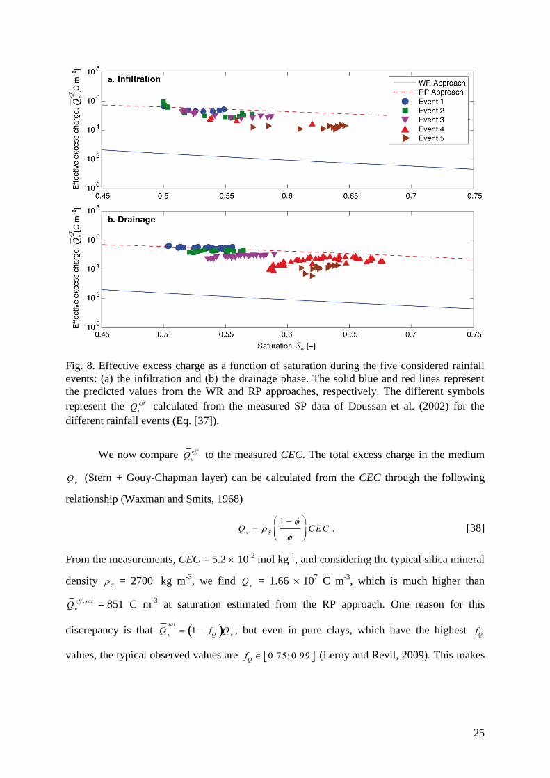
3.4 Simulation of the SP response to a rainfall event
We now compare the data of Doussan et al. (2002) with simulations of a single rainfall
event and the associated modeled SP response. The numerical simulations were conducted
using the finite element modeling software COMSOL Multiphysics 3.5 coupled with the
scientific computing environment MATLAB. In the simulation, the water flow was computed
using Richard’s equation with the van Genuchten parameterization (see Table 3 for the
parameter values). Note that the residual water content was set to w
r = 0.1 to reach
convergence of the hydrological problem at the beginning of the rainfall event. The source
current density was calculated from the computed Darcy velocity (Eq. [9]) and the Qv
eff(S
w)
was predicted using the RP approach. Considering the low conductivity of the rainwater (2.5
10-3
S m-1
), the transport was simulated to also take variations of the pore water
conductivity into account. The electrical conductivity model of Waxman and Smits (1968)
was used with the parameters of Doussan et al. (2002). The electrical problem (Eq. [3]) was
solved at different times to compute the SP signal arising from the hydrological simulation
results.
The simulation was performed considering a 2 m high and 0.05 m wide rectangle. The
measurement points correspond to the lysimeter experiment (depths of 0.3 and 0.4 m). The
geometry was discretized with a mesh with a side length smaller than 30 mm and a mesh
refinement down to 5 mm from the surface down to the two measurement points. The
hydrological boundary conditions were Neumann boundary conditions on the lateral sides (no
water flow), a constant water table at the bottom, and imposed flux at the top (Fig. 9a). The
system was assumed to be in hydrostatic equilibrium before the rainfall event with the initial
level of the water table determining the water content distribution in the medium. The
boundary conditions for the electrical problem were defined as a Neumann condition
(electrical insulation) with a reference ( = 0 V) at a depth of 0.30 m as in Doussan et al.,
(2002).
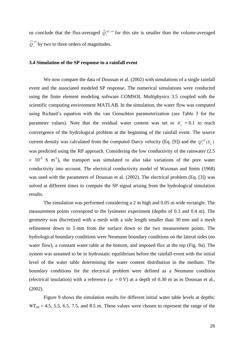
Figure 9 shows the simulation results for different initial water table levels at depths:
WTini = 4.5, 5.5, 6.5, 7.5, and 8.5 m. These values were chosen to represent the range of the
27
experimental hydraulic head of Doussan et al. (2002) prior to rainfall event 1 (day 91). The
imposed flux (Figure 9a) at the top corresponds to the rainfall intensity of event 1, which was
interpolated from hourly data measured in the vicinity of the lysimeter. Figure 9b shows the
variation of the matric potential at a depth of 0.35 m, while the corresponding SP signal
between 0.40 and 0.30 m depth is shown in Fig. 9c. The initial level of the water table has
clearly a strong influence on the SP response.
Fig. 9. Predicted SP signals due to rainfall for different initial water table levels: (a) imposed
flux from the climatic data of Doussan et al. (2002) for rainfall event 1 (day 91), (b) the
modeled matric potential at 35 cm, and (c) the SP signal between 30 and 40 cm depth. Sandy
Loam 1 and 2 SP data come from the lysimeter experiment of Doussan et al. (2002). The five
dashed lines in Fig 9c represent the predicted SP values for the approximation
Qv(S
w) Q
v
sat
Sw
.
The new proposed model explains the experimental data much better than the model
of Linde et al. (2007) (dashed lines in Fig. 9c). Considering WTini = 6.5 m, the normalized
28
RMS computed for the model based on the RP approach is 52.3 %, while the signal predicted
from the Linde et al. (2007) model has a RMS = 97.5 %. We believe that a better description
of the initial hydrological conditions would further improve the simulation results of the RP
approach. Indeed, it is unlikely to find a hydrostatic equilibrium in a natural soil under in-situ
conditions. In addition, evaporation processes were not taken into account in the modeling.
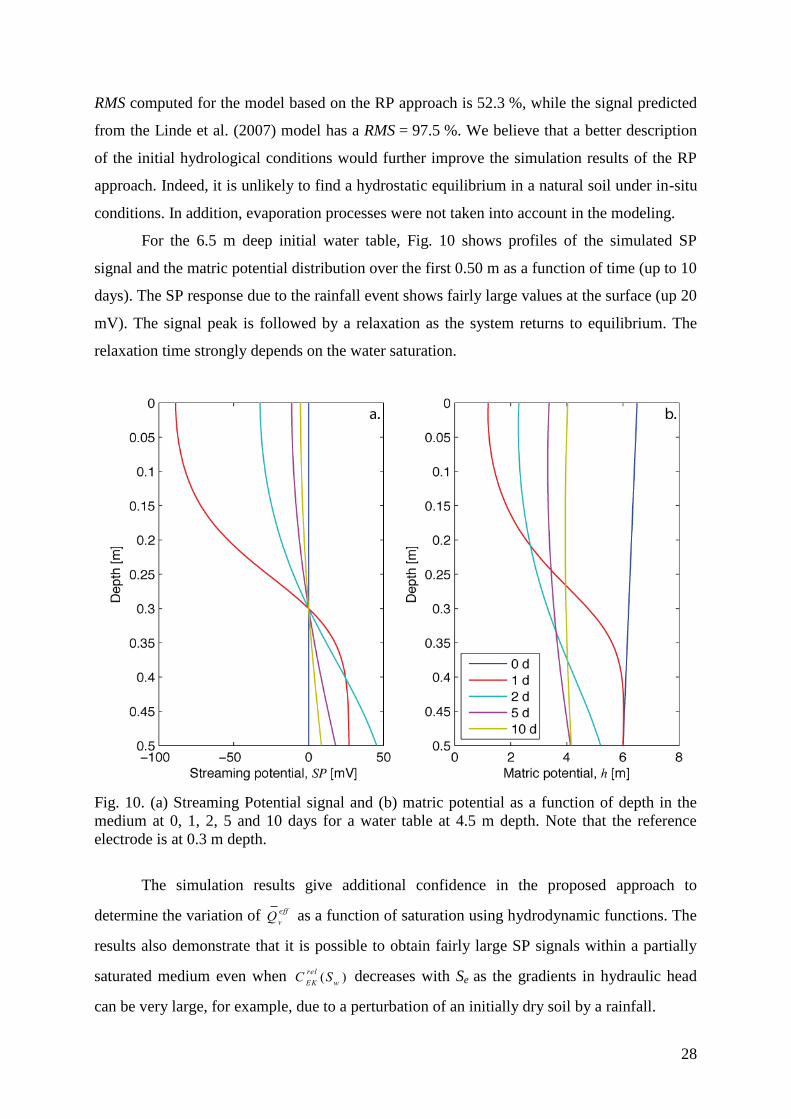
For the 6.5 m deep initial water table, Fig. 10 shows profiles of the simulated SP
signal and the matric potential distribution over the first 0.50 m as a function of time (up to 10
days). The SP response due to the rainfall event shows fairly large values at the surface (up 20
mV). The signal peak is followed by a relaxation as the system returns to equilibrium. The
relaxation time strongly depends on the water saturation.
Fig. 10. (a) Streaming Potential signal and (b) matric potential as a function of depth in the
medium at 0, 1, 2, 5 and 10 days for a water table at 4.5 m depth. Note that the reference
electrode is at 0.3 m depth.
The simulation results give additional confidence in the proposed approach to
determine the variation of Qv
eff as a function of saturation using hydrodynamic functions. The
results also demonstrate that it is possible to obtain fairly large SP signals within a partially
saturated medium even when CEK
rel(S
w) decreases with Se as the gradients in hydraulic head
can be very large, for example, due to a perturbation of an initially dry soil by a rainfall.
29
4. Discussion
The two new approaches to predict soil-specific flux-averaged Qv
eff(S
e) have a higher
predictive capacity than the model of Linde et al. (2007) and Revil et al. (2007). The primary
reason for this improvement is that the volume-averaging used in the latter approach is based
on the assumption of a uniform distribution of excess charge in the pore space. As shown in
Fig. 9, the predictions based on Qv(S
w) Q
v
satSw
is smaller than the measured SP signals by 3
to 4 orders of magnitude, while the RP approach provides values in the same order of
magnitude as the field data. This improvement is achieved by considering a more complex
model of Qv
eff(S
e) derived from hydrodynamic functions that explicitly considers that Q
v
eff(S
e)
is a flux-averaged property. We find that the RP approach is more reliable than the WR
approach, which nevertheless provide rather good results in terms of relative variations with
respect to water saturation. The better performance of the RP approach is likely caused by an
improved inference of the equivalent pore size distribution compared with the WR approach.
The numerical simulations highlight that the SP signals are strongly related to the
distribution of excess charge in the pore space and the velocity distribution in the pore space
(Fig. 1). The very important difference between the flux-averaged Qv
eff calculated from
experimental results (Fig. 8) and the volume-averaged excess charge Qv
determined from
CEC measurements (see section 3.3) is due to that a disproportionately large fraction of fluid
flow takes place outside of the diffuse Gouy-Chapman layer.
The results presented here explain how SP signals can significantly increase at low
saturation even if the streaming potential coupling coefficient tends to decrease with
saturation. This happens as the hydraulic head gradients in the unsaturated zone can be very
large and it is the combined effects of the coupling coefficient and the hydraulic head that
creates the SP signal for a 1-D system. Another explanation is offered by rewriting Eq. [37] as
Qv
eff(S
w)
(Sw
)u .
[39]
This equation is as Eq. [37] only valid under 1-D conditions. At low water saturations we
found (Fig. 3) that the increase in Qv
eff(S
w) might be larger than 1000 compared with
saturated conditions and there is nothing unusual about (Sw
) decreasing with a factor of 10
at lower saturations. This means that SP signals at low saturation might be as large as for
saturated conditions even when the flux is 10-4
times smaller.
30
Equation [39] also highlights why it is unrealistic to expect a linear relationship
between SP values and water flux over a large saturation range. Doussan et al. (2002) found
that the linear regression models between SP values and water flux could be improved by
considering the water content. They attribute this to variations in electrode contact, but is
more likely caused by improved linearizations of the underlying non-linear relationship. The
difference in the predictions compared with volume averaging is about 100 at low water
saturations. This discrepancy explains why Linde et al. (2011) could not simulate the
observed SP magnitudes observed on a gravel bar following rainfall. The increased sensitivity
to water flow under unsaturated conditions might explain the slow and often incomplete
relaxation of SP signals following drainage (e.g. Allègre et al., 2010).
Our findings open up exciting possibilities of using the SP method to monitor very
small flows at low saturations, such as those due to evaporation. This would necessitate co-
located measurements of bulk electrical conductivity, water saturation, and a good description
of hydrodynamic soil properties.
5. Conclusions
Soil-specific water retention and relative permeability functions together with a
relative conductivity function are needed to predict the streaming potential coupling
coefficient under unsaturated conditions and hence SP signals. Most previous studies has
ignored or severely underestimated the importance of accurately modeling the scaling of the
effective excess charge, which we here predict from the above-mentioned soil-specific
hydrodynamic functions. Using a capillary tube model, we find that the effective (flux-
averaged) excess charge is for typical soils two-to-three orders of magnitude larger than
volume-averaged estimates, which translate to equally larger SP signals. The improvement
with respect to existing theory is demonstrated against laboratory data and by comparing the
modeled SP response caused by precipitation on a sandy loam with field data. For this data
set, the initial water content, the water retention and relative permeability, as well as relative
conductivity function was independently measured in the laboratory. The new theory predicts
both the right magnitudes and the slow relaxation of the observed SP signal, while this was
not possible using volume averaging. It is of course an advantage to have access to laboratory
or in situ measurements of hydrodynamic functions, but the presented predictions based on
the Carsel and Parrish (1988) database provide a rather good idea about the expected
variations of Qv
eff , rel(S
w) for different soil types.

31
Our work provide a credible explanation for the often surprisingly large SP signals
that are observed at low water saturation and it opens up the perspective of using SP signals to
characterize film flow and evaporation processes. It also suggests that SP signals in the
vadose zone can become a useful data source when estimating fluxes (or at least flux
directions) in the unsaturated zone and for inverse modeling applications. It also highlights
the importance of considering vadose zone processes in general SP surveys as flows that are
10-4
-10-5
times smaller than under saturated conditions may in dry soils lead to SP gradients
of the same magnitude.
Acknowledgments
We would like to thank Dani Or for some very useful suggestions in the early stages
of this research. Financial support from Fondation Herbette is gratefully acknowledged. We
thank Associate Editor Alex Furman and the three anonymous reviewers for detailed
comments that helped us to improve the paper.

32
Notations
Symbol Description Units
Electrical and electrochemical variables
ci
0 Ionic concentration of the species i in the free electrolyte mol m-3
ci Ionic concentration of species i mol m
-3
CEK
Streaming potential coupling coefficient V Pa-1
CEC Cation Exchange Capacity mol kg-1
E Electrical field V m-1
fQ Fraction of the excess charge in the Stern layer -
F Electrical formation factor -
I Ionic strength mol m-3
j Total current density A m-2
js Source current density A m-2
lD Debye length m
m Electrical cementation index -
n Electrical saturation index -
N Number of ionic species i -
qi Charge of the ionic species i C
Qv Volumetric excess charge C m
-3
Qv Volume averaged excess charge C m
-3
Qv
eff Effective volumetric excess charge C m-3
T Temperature K
zi Ionic valence of the species i -
Dielectric permittivity F m-1
r Relative dielectric permittivity of water -
Angular frequency Hz
Electrical potential of the porous medium V
Local electrical potential in the pore water V
Electrical conductivity of the medium S m-1
w
Water electrical conductivity S m-1
S Surface electrical conductivity S m
-1
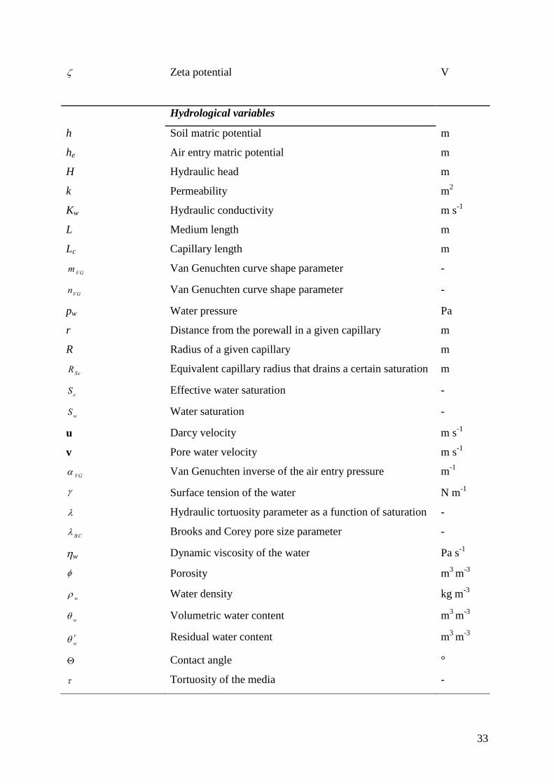
33
Zeta potential V
Hydrological variables
h Soil matric potential m
he Air entry matric potential m
H Hydraulic head m
k Permeability m2
Kw Hydraulic conductivity m s-1
L Medium length m
Lc Capillary length m
mVG
Van Genuchten curve shape parameter -
nVG
Van Genuchten curve shape parameter -
pw Water pressure Pa
r Distance from the porewall in a given capillary m
R Radius of a given capillary m
RSe
Equivalent capillary radius that drains a certain saturation m
Se Effective water saturation -
Sw
Water saturation -
u Darcy velocity m s-1
v Pore water velocity m s-1
VG
Van Genuchten inverse of the air entry pressure m-1
Surface tension of the water N m-1
Hydraulic tortuosity parameter as a function of saturation -
BC
Brooks and Corey pore size parameter -
w Dynamic viscosity of the water Pa s-1
Porosity m3
m-3
w Water density kg m
-3
w
Volumetric water content m3
m-3
w
r Residual water content m3
m-3
Contact angle °
Tortuosity of the media -
34
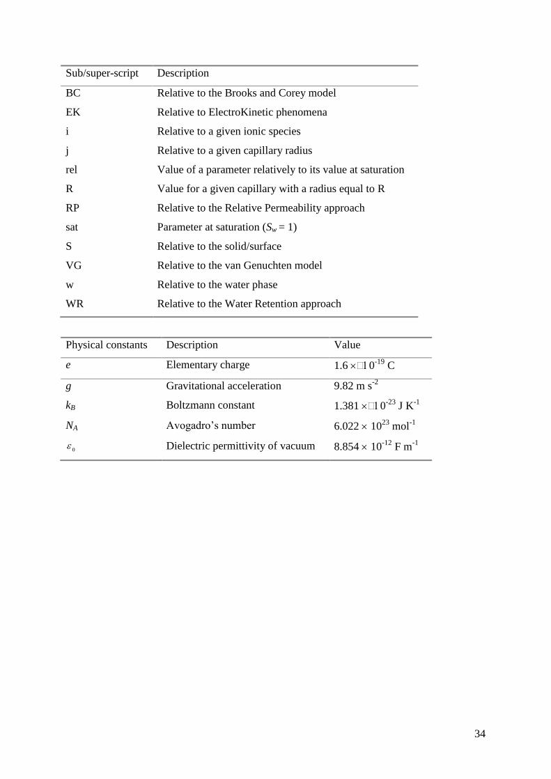
Sub/super-script Description
BC Relative to the Brooks and Corey model
EK Relative to ElectroKinetic phenomena
i Relative to a given ionic species
j Relative to a given capillary radius
rel Value of a parameter relatively to its value at saturation
R Value for a given capillary with a radius equal to R
RP Relative to the Relative Permeability approach
sat Parameter at saturation (Sw = 1)
S Relative to the solid/surface
VG Relative to the van Genuchten model
w Relative to the water phase
WR Relative to the Water Retention approach
Physical constants Description Value
e Elementary charge 1.6 0-19
C
g Gravitational acceleration 9.82 m s-2
kB Boltzmann constant 1.381 0-23
J K-1
NA Avogadro’s number 6.022 1023
mol-1
0 Dielectric permittivity of vacuum 8.854 10
-12 F m
-1
35
References
Archie, G.E. 1942. The electrical resistivity as an aid in determining some reservoir
characteristics. Trans. AIME 146:54–62.
Allègre, V., L. Jouniaux, F. Lehmann, and P. Sailhac. 2010. Streaming potential dependence
on water-content in Fontainebleau sand. Geophys. J. Int. 182:1248–1266.
Allègre, V., L. Jouniaux, F. Lehmann, and P. Sailhac. 2011. Reply to comment by A. Revil
and N. Linde on ‘Streaming potential dependence on water-content in Fontainebleau
sand’. Geophys. J. Int. 186:115-117.
Bear, J. 1972. Dynamics of fluids in porous media. Elsevier, Amsterdam.
Bolève, A., A. Crespy, A. Revil, F. Janod, J.L. Mattiuzzo. 2007. Streaming potentials of
granular media: Influence of the Dukhin and Reynolds numbers. J. Geophys. Res.
112:B08204.
Brooks, R.H., and A.T. Corey. 1964. Hydraulic Properties of Porous Media. Hydrol. Pap. 3,
Colorado State Univ., Fort Collins.
Carsel, R.F., and R.S. Parrish. 1988. Developing joint probability distributions of soil water
retention characteristics. Water Resour. Res. 24:755-769.
Darnet, G., and G. Marquis. 2004. Modelling streaming potential (SP) signals induced by
water movement in the vadose zone. J. Hydrol. 285:114-124.
Doussan, C., L. Jouniaux, and J. L. Thony. 2002. Variations of self-potential and unsaturated
water flow with time in sandy loam and clay loam soils. J. Hydrol. 267:173-185.
Doussan, C., and S. Ruy. 2009. Prediction of unsaturated soil hydraulic conductivity with
electrical conductivity. Water Resour. Res. 45:W10408.
Everett, M.E., and M.A. Meju. 2005. Near-Surface controlled-source electromagnetic
induction: background and recent advances, p.157-184. In Y. Rubin and S.S. Hubbard
(ed.) Hydrogeophysics. Springer, Dordrecht, the Netherlands.
Gonçalvès, J., P. Rousseau-Gueutin, and A. Revil. 2007. Introducing interacting diffuse layers
in TLM calculations: A reappraisal of the influence of the pore size on the swelling
pressure and the osmotic efficiency of compacted bentonites. J. Colloid Interf. Sci.
316:92–99.
Guichet, X., L. Jouniaux, and J.-P. Pozzi. 2003. Streaming potential of a sand column in
partial saturation conditions. J. Geoph. Res. 108:B32141.
36
Günther, T., C. Rücker, and K. Spitzer. 2006. Three-dimensional modeling and inversion of
dc resistivity data incorporating topography – II. Inversion. Geophys. J. Int. 166:506–
517.
Haas, A., and A. Revil. 2009. Electrical burst signature of pore-scale displacements. Water
Resour. Res. 45:W10202.
Hunter, R.J. 1981. Zeta potential in colloid sciences: principles and applications. Academic
Press, New York.
Jackson, M.D. 2008. Characterization of multiphase electrokinetic coupling using a bundle of
capillary tubes model. J. Geophys. Res. 113:B04201.
Jackson, M.D. 2010. Multiphase electrokinetic coupling: Insights into the impact of fluid and
charge distribution at the pore scale from a bundle of capillary tubes model. J. Geoph.
Res. 115:B07206.
Jardani, A., A. Revil, A. Bolève, J.P. Dupont, W. Barrash, and B. Malama. 2007.
Tomography of groundwater flow from self-potential (SP) data. Geophys. Res. Lett.
34:L24403.
Jouniaux, L., and J.-P. Pozzi. 1997. Anomalous 0.1– 0.5 Hz streaming potential
measurements under geochemical changes: Consequences for electrotelluric precursors
to earthquakes. J. Geophys. Res. 102:15335–15343.
Jury, W.A., W.R. Gardner, and W.H. Gardner. 1991. Soil Physics. John Wiley and Sons, New
York, NY.
Knight, R. 1991. Hysteresis in the electrical resistivity of partially saturated sandstones.
Geophysics, 56:2139-2147.
Kowalsky, M.B., S. Finsterle, J. Peterson, S. Hubbard, Y. Rubin, E. Majer, A. Ward, and G.
Gee. 2005. Estimation of field-scale soil hydraulic and dielectric parameters through
joint inversion of GPR and hydrological data. Water Resour. Res. 41:W11425.
Laloy, E., M. Javaux, M. Vanclooster, C. Roisin, and C.L. Bielders. 2011. Electrical resistivity in
a loamy soil: identification of the appropriate pedo-electrical model, Vadose Zone J. 10:1-
11.
Leroy, P., and A. Revil. 2004. A triple-layer model of the surface electrochemical properties
of clay minerals. J. Colloid Interface Sci. 270(2):371–380.
Leroy, P., and A. Revil. 2009. A mechanistic model for the spectral induced polarization of
clay materials. J. Geophys. Res. 114:B10202.
37
Lesmes, D.P., and S.P. Friedman. 2005. Relationships between the electrical and
hydrogeological properties of rocks and soils. P. 87–128. In Y. Rubin and S.S. Hubbard
(ed.) Hydrogeophysics. Springer, Dordrecht, the Netherlands.
Linde, N. 2009. Comment on ―Characterization of multiphase electrokinetic coupling using a
bundle of capillary tubes model’’ by Mathew D. Jackson. J. Geophys. Res. 114:B06209.
Linde, N., J. Doetsch, D. Jougnot, O. Genoni, Y. Dürst, B. J. Minsley, T. Vogt, N. Pasquale,
and J. Luster. 2011. Self-potential investigations of a gravel bar in a restored river
corridor. Hydrol. Earth Syst. Sci. 15:729–742.
Linde, N., D. Jougnot, A. Revil, S.K. Matthaï, T. Arora, D. Renard, and C. Doussan. 2007.
Streaming current generation in two-phase flow conditions. Geophys. Res. Lett.
34(3):L03306.
Maineult, A., E. Strobach, and J. Renner. 2008. Self-potential signals induced by periodic
pumping tests. J. Geophys. Res. 113:B01203.
Metson, A.J. 1956. Methods of chemical analysis for soil survey samples. NZ Soil Bur Bull
12.
Minsley, B.J. 2007. Modeling and inversion of self-potential data. Ph.D. diss. Massachusetts
Institute of Technology.
Mualem, Y. 1976. A new model for predicting the hydraulic conductivity of unsaturated
porous media. Water Resour. Res. 12:513-522.
Mualem, Y. 1984. A modified dependent-domain theory of hysteresis. Soil Sci. 137(5):283–
291.
Pengra, D.B., S.X. Li, and P.-Z.Wong. 1999. Determination of rock properties by low-
frequency AC electrokinetics. J. Geophys. Res. 104:29485–29508.
Perrier, F., and P. Morat. 2000. Characterization of electrical daily variations induced by
capillary flow in the non-saturated zone. Pure Appl. Geophys. 157:785-810.
Petiau, G. 2000. Second generation of lead-lead chloride electrodes for geophysical
applications. Pure Appl. Geophys. 157:357-382.
Pride, S. 1994. Governing equations for the coupled electromagnetics and acoustics of porous
media. Phys. Rev. B 50(21):15678-15696.
Revil, A., and A. Cerepi. 2004. Streaming potential in two-phase flow condition. Geophys.
Res. Letters 31(11):L11605.
Revil, A., C. Gevaudan, N. Lu, and A. Maineult. 2008. Hysteresis of the self-potential
response associated with harmonic pumping tests. Geophys. Res. Lett. 35:L16402.
38
Revil, A., D. Hermitte, E. Spangenberg, and J.J. Cochémé. 2002. Electrical properties of
zeolitized volcaniclastic materials. J. Geophys. Res. 107(B8):2168.
Revil, A., and P. Leroy. 2004. Constitutive equations for ionic transport in porous shales. J.
Geophys. Res. 109:B03208.
Revil, A., P. Leroy, and K. Titov. 2005. Characterization of transport properties of
argillaceous sediments: Application to the Callovo-Oxfordian argillite. J. Geophys. Res.
110:B06202.
Revil, A., N. Linde, A. Cerepi, D. Jougnot, S. Matthäi, and S. Finsterle. 2007. Electrokinetic
coupling in unsaturated porous media. J. Colloid Interf. Sci. 313(1):315-327.
Revil, A. and N. Linde 2006. Chemico-electromechanical coupling in microporous media. J.
Colloid Interf. Sci. 302:682–694.
Revil, A., P.A. Pezard, and P.W.J. Glover. 1999. Streaming potential in porous media, 1.
Theory of the zeta potential. J. Geophys. Res. 104(B9):20021-20031.
Revil, A., F. Trolard, G. Bourrié, J. Castermant, A. Jardani, and C.A. Mendonça. 2009. Ionic
contribution to the self-potential signals associated with a redox front. J. Contam.
Hydrol. 109:27–39.
Rhoades, J.D., N. A. Manteghi, P.J. Shouse, and W.J. Alves. 1989. Soil electrical
conductivity and soil salinity: new formulations and calibrations. Soil Sci. Soc. Am. J.
53:433–439.
Sailhac, P., M. Darnet, G. Marquis. 2004. Electrical streaming potential measured at the
ground surface: Forward modeling and inversion issues for monitoring infiltration and
characterizing the vadose zone. Vadose Zone J. 3(4):1200-1206.
Saunders, J.H., M.D. Jackson, and C.C. Pain. 2006. A new numerical model of electrokinetic
potential response during hydrocarbon recovery. Geophys. Res. Lett. 33:L15316.
Sill, W.R. 1983. Self-potential modeling from primary flows. Geophysics. 48:76-86.
Sheffer, M. 2007. Forward modeling and inversion of streaming potential for the
interpretation of hydraulic conditions from self-potential data. PhD diss. The University
of British Columbia.
Suski, B., A. Revil, K. Titov, P. Konosavsky, M. Voltz, C. Dages, and O. Huttel. 2006.
Monitoring of an infiltration experiment using the self-potential method. Water Resour.
Res. 42:W08418.
Tamari, S., L. Bruckler, J. Halbertsma, and J. Chadoeuf. 1993. A simple method for
determining soil hydraulic properties in the laboratory. Soil Sci. Soc. Am. J. 57:642–
651.
39
Tarantino, A., A.M. Ridley, and D.G. Toll. 2008. Field measurement of suction, water
content, and water permeability. Geotech. Geol. Eng. 26:751–782.
Tournassat, C., Y. Chapron, P. Leroy , M. Bizi, F. Boulahya. 2009. Comparison of molecular
dynamics simulations with triple layer and modified Gouy–Chapman models in a 0.1 M
NaCl–montmorillonite system. J. Colloid Interface Sci. 339:533–541.
Thony, J.L., P. Morat, G. Vachaud, and J.L. Le Mouël. 1997. Field characterization of the
relationship between electrical potential gradients and soil water flux. CR Acad. Sci. II
A 325:317-325.
Van Genuchten, M. T. 1980. A closed-form equation for predicting the hydraulic conductivity
of unsaturated soils. Soil Sci. Soc. 44:892-898.
Vereecken, H., J.A. Huisman, H. Bogena, J. Vanderborght, J.A. Vrugt, and J.W. Hopmans.
2008. On the value of soil moisture measurements in vadose zone hydrology: A review.
Water Resour. Res. 44 :W00D06.
Vinogradov, J., and M.D. Jackson. 2010. Multiphase streaming potential in sandstones
saturated with gas/brine and oil/brine during drainage and imbibition. Geophys. Res.
Lett. 11(38):L01301.
Waxman, M.M., and L.J.M. Smits. 1968. Electrical conductivity in oil-bearing shaly sand.
Soc. Pet. Eng. J. 463(8):107-122.
Worthington, A.E., J.H. Hedges, and N. Pallatt. 1990. SCA guidelines for sample preparation
and porosity measurement of electrical resistivity samples: Part I–Guidelines for
preparation of brine and determination of brine resistivity for use in electrical resistivity
measurements. The Log Analyst 31:20.
Wurmstich, B. and F.D. Morgan. 1994. Modeling of streaming potential responses caused by
oil well pumping. Geophysics. 59(1):46-56.