2-1

Chapter 2 Thermoelectric

Generators

2.1 Ideal Equations

In 1821, Thomas J. Seebeck discovered that an electromotive force or potential difference could

be produced by a circuit made from two dissimilar wires when one junction was heated. This is

called the Seebeck effect. In 1834, Jean Peltier discovered the reverse process that the passage of

an electric current through a thermocouple produces heating or cooling depended on its direction

[1]. This is called the Peltier effect (or Peltier cooling). In 1854, William Thomson discovered

that if a temperature difference exists between any two points of a current-carrying conductor,

heat is either absorbed or liberated depending on the direction of current and material [2]. This is

called the Thomson effect (or Thomson heat). These three effects are called the thermoelectric

effects.

Let us consider a non-uniformly heated thermoelectric material. For an isotropic substance, the

continuity equation for a constant current gives

∇⃑⃑ ∙ 𝑗 = 0 (2.1)

2-2

The electric field E

is affected by the current density j

and the temperature gradient T

. The

coefficients are known according to the Ohm’s law and the Seebeck effect [3]. The electric field

is then expressed as

TjE

(2.2)

The heat flux q

is also affected by both the field E

and the temperature gradient T

. However,

the coefficients were not readily attainable at that time. Thomson in 1854 arrived at the

relationship assuming that thermoelectric phenomena and thermal conduction are independent

[2]. Later, Onsager [4] supported that relationship by presenting the reciprocal principle which

was experimentally proved. The Thomson relationship and the Onsager’s principle yielded the

heat flow density vector (heat flux), which is expressed as

TkjTq

(2.3)

which is the most important equation in thermoelectrics (will be discussed later in detail). The

general heat diffusion equation is given by

t

Tcqq p

(2.4)

For steady state, we have

0 qq

(2.5)

where q is expressed by [3]

2-3

TjjjEq

2 (2.6)

Substituting Equation (2.3) and (2.6) into (2.5) yields

02 TjdT

dTjTk

(2.7)

The Thomson coefficient , originally obtained from the Thomson relations, is written by

dT

dT

(2.8)

In Equation (2.7), the first term is the thermal conduction, the second term is the Joule heating,

and the third term is the Thomson heat. Note that if the Seebeck coefficient is independent of

temperature, the Thomson coefficient becomes zero and then the Thomson heat is absent. The

two equations (2.3) and (2.7) governs the thermoelectric phenomena.

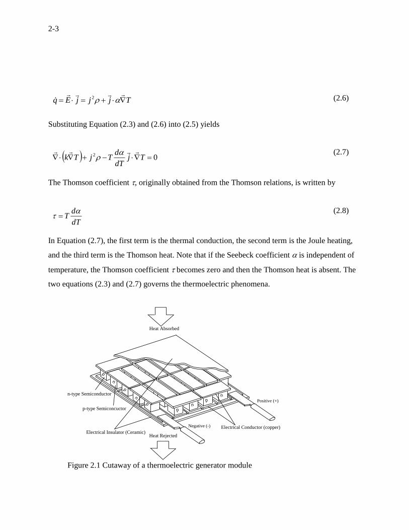
Figure 2.1 Cutaway of a thermoelectric generator module

p

n

p

n

np

p

pn

Positive (+)

Negative (-)

Heat Absorbed

Heat Rejected

Electrical Conductor (copper)Electrical Insulator (Ceramic)

p-type Semiconcuctor

n-type Semiconductor

2-4

(b)

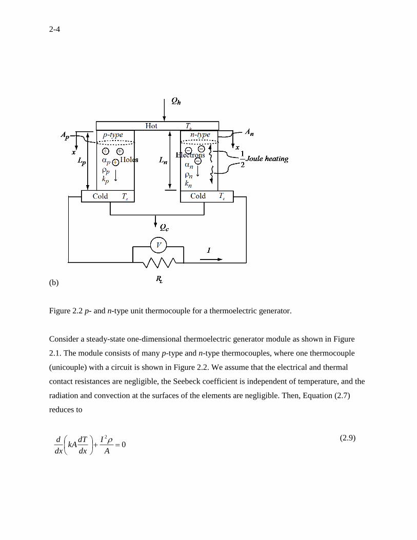
Figure 2.2 p- and n-type unit thermocouple for a thermoelectric generator.

Consider a steady-state one-dimensional thermoelectric generator module as shown in Figure

2.1. The module consists of many p-type and n-type thermocouples, where one thermocouple

(unicouple) with a circuit is shown in Figure 2.2. We assume that the electrical and thermal

contact resistances are negligible, the Seebeck coefficient is independent of temperature, and the

radiation and convection at the surfaces of the elements are negligible. Then, Equation (2.7)

reduces to

02

A

I

dx

dTkA

dx

d

(2.9)

2-5

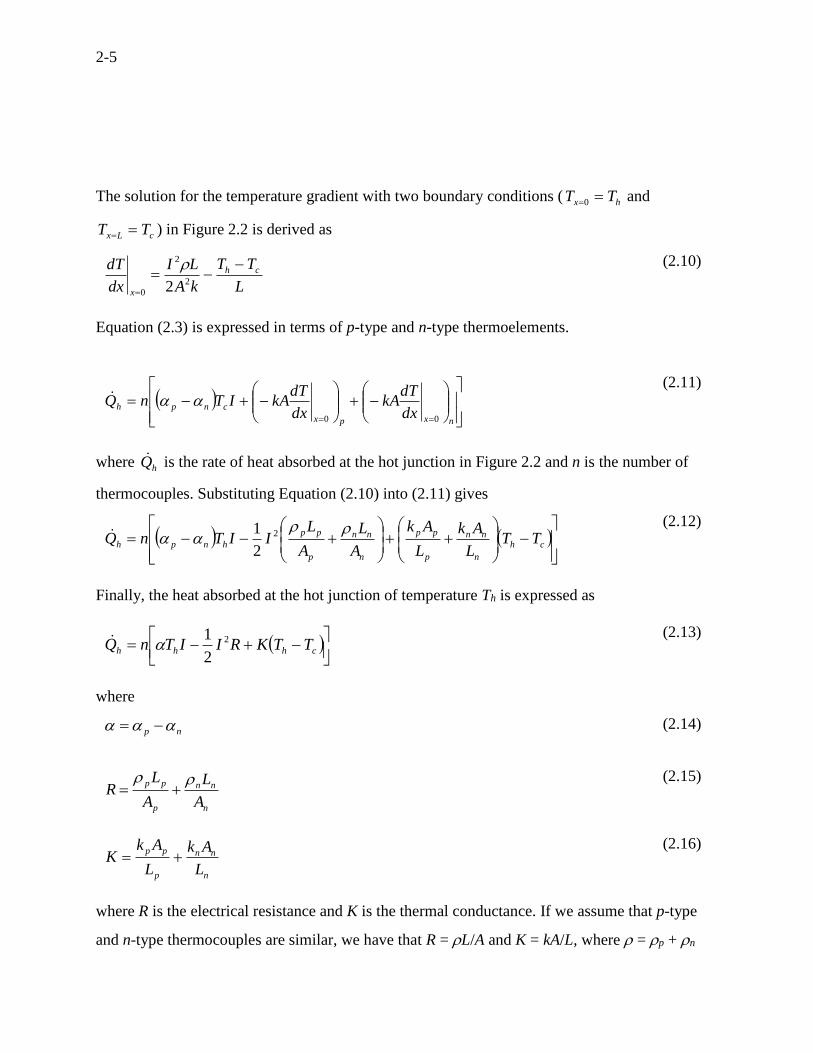
The solution for the temperature gradient with two boundary conditions ( hx TT 0 and

cLx TT ) in Figure 2.2 is derived as

L

TT

kA

LI

dx

dT ch

x

2

2

0 2

(2.10)

Equation (2.3) is expressed in terms of p-type and n-type thermoelements.

nxpx

cnphdx

dTkA

dx

dTkAITnQ

00

(2.11)

where hQ is the rate of heat absorbed at the hot junction in Figure 2.2 and n is the number of

thermocouples. Substituting Equation (2.10) into (2.11) gives

ch

n

nn

p

pp

n

nn

p

pp

hnph TTL

Ak

L

Ak

A

L

A

LIITnQ

2

2

1 (2.12)

Finally, the heat absorbed at the hot junction of temperature Th is expressed as

chhh TTKRIITnQ 2

2

1

(2.13)

where

np (2.14)

n

nn

p

pp

A

L

A

LR

(2.15)

n

nn

p

pp

L

Ak

L

AkK

(2.16)

where R is the electrical resistance and K is the thermal conductance. If we assume that p-type

and n-type thermocouples are similar, we have that R = L/A and K = kA/L, where = p + n

2-6

and k = kp + kn. Equation (2.13) is called the ideal equation which has been widely used in

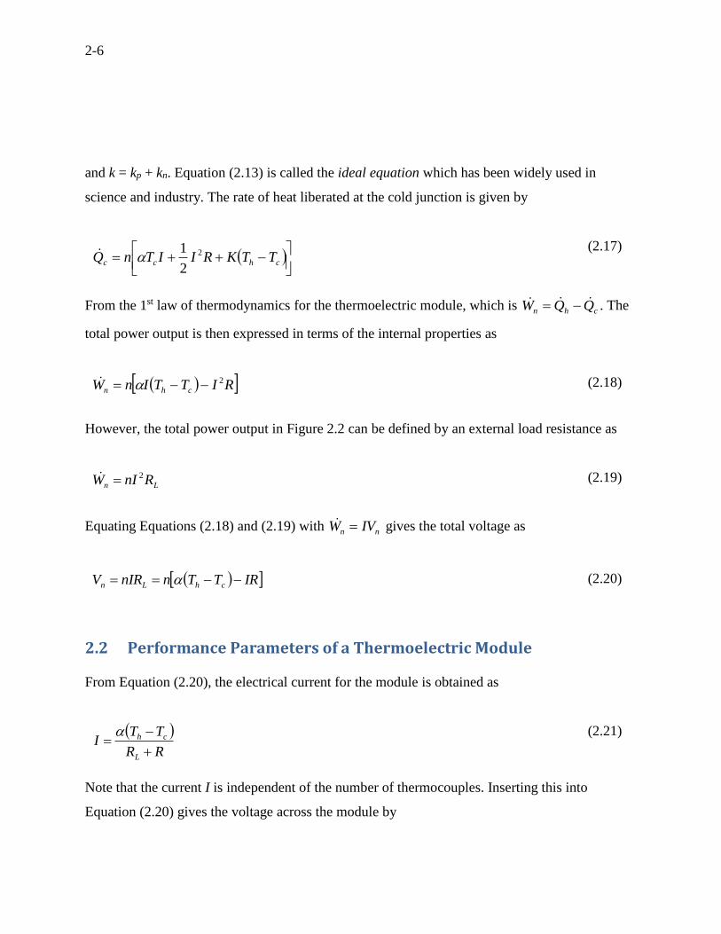
science and industry. The rate of heat liberated at the cold junction is given by

chcc TTKRIITnQ 2

2

1

(2.17)

From the 1st law of thermodynamics for the thermoelectric module, which is chn QQW . The

total power output is then expressed in terms of the internal properties as

RITTInW chn

2 (2.18)

However, the total power output in Figure 2.2 can be defined by an external load resistance as

Ln RnIW 2 (2.19)

Equating Equations (2.18) and (2.19) with nn IVW gives the total voltage as

IRTTnnIRV chLn (2.20)

2.2 Performance Parameters of a Thermoelectric Module

From Equation (2.20), the electrical current for the module is obtained as

RR

TTI

L

ch

(2.21)

Note that the current I is independent of the number of thermocouples. Inserting this into

Equation (2.20) gives the voltage across the module by

2-7

R

R

R

R

TTnV L

L

chn

1

(2.22)

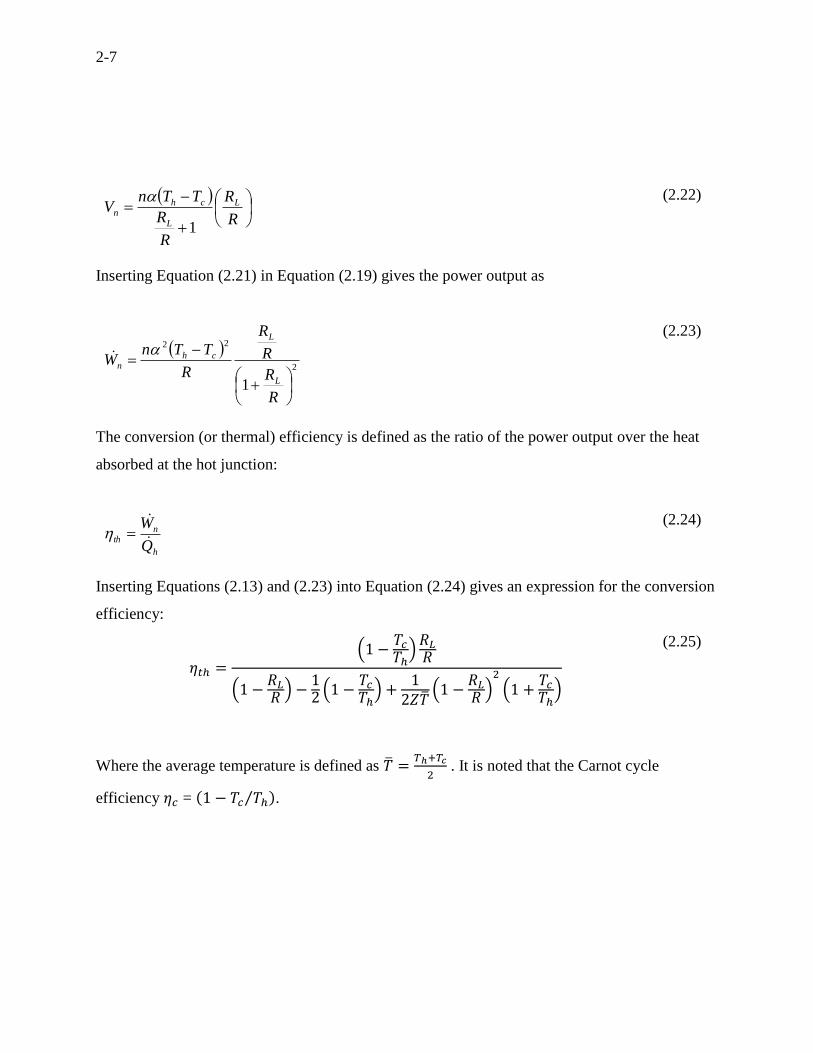
Inserting Equation (2.21) in Equation (2.19) gives the power output as

2

22

1

R

R

R

R

R

TTnW

L

L

chn

(2.23)

The conversion (or thermal) efficiency is defined as the ratio of the power output over the heat

absorbed at the hot junction:

h

nth

Q

W

(2.24)

Inserting Equations (2.13) and (2.23) into Equation (2.24) gives an expression for the conversion

efficiency:

𝜂𝑡ℎ =(1 −

𝑇𝑐

𝑇ℎ)𝑅𝐿

𝑅

(1 −𝑅𝐿

𝑅 ) −12 (1 −

𝑇𝑐

𝑇ℎ) +

12𝑍�̅�

(1 −𝑅𝐿

𝑅 )2

(1 +𝑇𝑐

𝑇ℎ)

(2.25)

Where the average temperature is defined as �̅� =𝑇ℎ+𝑇𝑐

2 . It is noted that the Carnot cycle

efficiency 𝜂𝑐 = (1 − 𝑇𝑐 𝑇ℎ⁄ ).

2-8

2.3 Maximum Parameters for a thermoelectric Module

Since the maximum current inherently occurs at the short circuit where 0LR in Equation (2.21),

the maximum current for the module is

R

TTI ch

max

(2.26)

The maximum voltage inherently occurs at the open circuit where I = 0 in Equation (2.20). The

maximum voltage is

ch TTnV max (2.27)

The maximum power output is attained by differentiating the power output W in Equation (2.23)

with respect to the ratio of the load resistance to the internal resistance and setting it to zero. The

result yields a relationship of 1RRL , which leads to the maximum power output as

R

TTnW ch

4

22

max

(2.28)

The maximum conversion efficiency can be obtained by differentiating the conversion efficiency

in Equation (2.25) with respect to the ratio of the load resistance to the internal resistance and

setting it to zero. The result yields a relationship of TZRRL 1 . Then, the maximum

conversion efficiency max is

h

ch

c

T

TTZ

TZ

T

T

1

111max

(2.29)

2-9

There are total four essential maximum parameters, which are maxI , maxV , maxW , and max .

However, there is also the maximum power efficiency. The maximum power efficiency is obtained

by letting 1RRL in Equation (2.25). The maximum power efficiency mp is

𝜂𝑚𝑝 =(1 −

𝑇𝑐

𝑇ℎ)

2 −12 (1 −

𝑇𝑐

𝑇ℎ) +

2𝑍�̅�

(1 +𝑇𝑐

𝑇ℎ)

(2.30)

Note there are two thermal efficiencies: the maximum power efficiency mp and the maximum

conversion efficiency max .

2.4 Normalized Parameters

If we divide the actual values by the maximum values, we can normalize the characteristics of a

thermoelectric generator. The normalized power output can be obtained by dividing Equation

(2.23) by Equation (2.28), which leads to

2

max1

4

R

R

R

R

W

W

L

L

(2.31)

Equations (2.21) and (2.26) give the normalized currents as

1

1

max

R

RI

I

L

(2.32)

Equations (2.22) and (2.27) give the normalized voltage as

2-10

1max

R

RR

R

V

V

L

L

n

(2.33)

Equations (2.25) and (2.29) give the normalized thermal efficiency as

𝜂𝑡ℎ

𝜂𝑚𝑎𝑥=

𝑅𝐿

𝑅 (√1 + 𝑍�̅� +𝑇𝑐

𝑇ℎ)

[(𝑅𝐿

𝑅 + 1) −12 (1 −

𝑇𝑐

𝑇ℎ) +

12𝑍�̅�

(𝑅𝐿

𝑅 + 1)2

(1 +𝑇𝑐

𝑇ℎ)] (√1 + 𝑍�̅� − 1)

(2.34)

Note that the normalized values in Equations (2.31) – (2.33) are a function only of RRL , while

Equation (2.34) is a function of three parameters, which are hc TT , RRL and 𝑍�̅�.

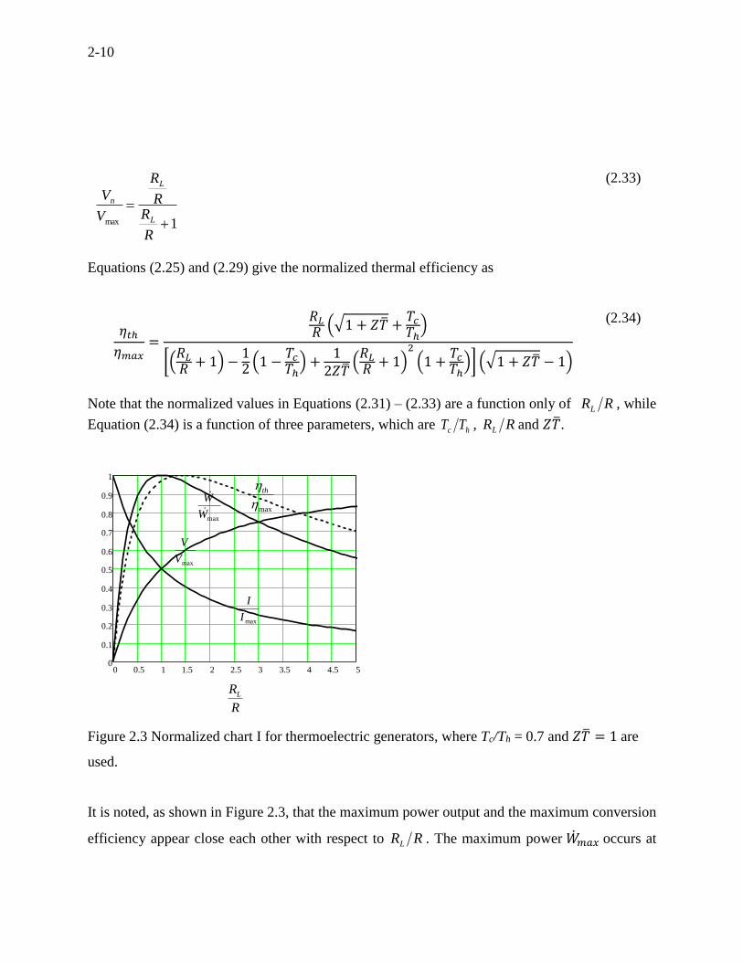
Figure 2.3 Normalized chart I for thermoelectric generators, where Tc/Th = 0.7 and 𝑍�̅� = 1 are

used.

It is noted, as shown in Figure 2.3, that the maximum power output and the maximum conversion

efficiency appear close each other with respect to RRL . The maximum power �̇�𝑚𝑎𝑥 occurs at

0 0.5 1 1.5 2 2.5 3 3.5 4 4.5 50

0.1

0.2

0.3

0.4

0.5

0.6

0.7

0.8

0.9

1

max

th

maxW

W

maxV

V

maxI

I

R

RL

2-11

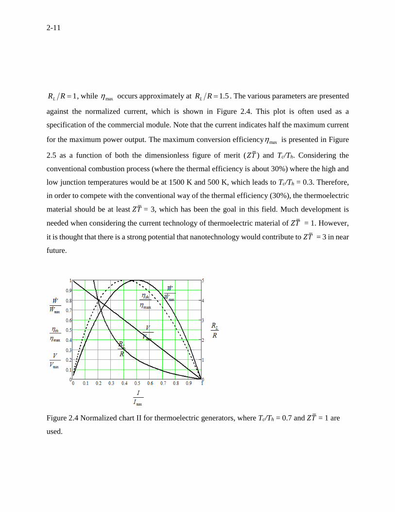
1RRL , while max occurs approximately at 5.1RRL . The various parameters are presented

against the normalized current, which is shown in Figure 2.4. This plot is often used as a

specification of the commercial module. Note that the current indicates half the maximum current

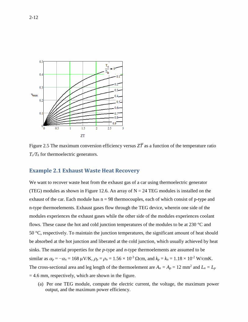
for the maximum power output. The maximum conversion efficiency max is presented in Figure

2.5 as a function of both the dimensionless figure of merit (𝑍�̅�) and Tc/Th. Considering the

conventional combustion process (where the thermal efficiency is about 30%) where the high and

low junction temperatures would be at 1500 K and 500 K, which leads to Tc/Th = 0.3. Therefore,

in order to compete with the conventional way of the thermal efficiency (30%), the thermoelectric

material should be at least 𝑍�̅� = 3, which has been the goal in this field. Much development is

needed when considering the current technology of thermoelectric material of 𝑍�̅� = 1. However,

it is thought that there is a strong potential that nanotechnology would contribute to 𝑍�̅� = 3 in near

future.

Figure 2.4 Normalized chart II for thermoelectric generators, where Tc/Th = 0.7 and 𝑍�̅� = 1 are

used.

2-12

Figure 2.5 The maximum conversion efficiency versus 𝑍𝑇 ̅as a function of the temperature ratio

Tc/Th for thermoelectric generators.

Example 2.1 Exhaust Waste Heat Recovery

We want to recover waste heat from the exhaust gas of a car using thermoelectric generator

(TEG) modules as shown in Figure 12.6. An array of N = 24 TEG modules is installed on the

exhaust of the car. Each module has n = 98 thermocouples, each of which consist of p-type and

n-type thermoelements. Exhaust gases flow through the TEG device, wherein one side of the

modules experiences the exhaust gases while the other side of the modules experiences coolant

flows. These cause the hot and cold junction temperatures of the modules to be at 230 °C and

50 °C, respectively. To maintain the junction temperatures, the significant amount of heat should

be absorbed at the hot junction and liberated at the cold junction, which usually achieved by heat

sinks. The material properties for the p-type and n-type thermoelements are assumed to be

similar as p = −n = 168 V/K, p = n = 1.56 × 10-3 cm, and kp = kn = 1.18 × 10-2 W/cmK.

The cross-sectional area and leg length of the thermoelement are An = Ap = 12 mm2 and Ln = Lp

= 4.6 mm, respectively, which are shown in the figure.

(a) Per one TEG module, compute the electric current, the voltage, the maximum power

output, and the maximum power efficiency.

2-13

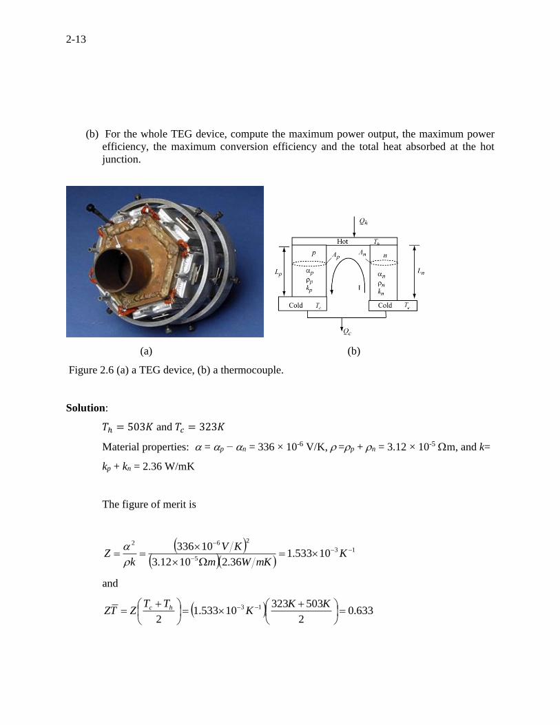
(b) For the whole TEG device, compute the maximum power output, the maximum power

efficiency, the maximum conversion efficiency and the total heat absorbed at the hot

junction.

(a) (b)

Figure 2.6 (a) a TEG device, (b) a thermocouple.

Solution:

𝑇ℎ = 503𝐾 and 𝑇𝑐 = 323𝐾

Material properties: =p − n = 336 × 10-6 V/K, =p + n = 3.12 × 10-5 m, and k=

kp + kn = 2.36 W/mK

The figure of merit is

13

5

262

10533.136.21012.3

10336

K

mKWm

KV

kZ

and

633.02

50332310533.1

2

13

KK

KTT

ZTZ hc

2-14

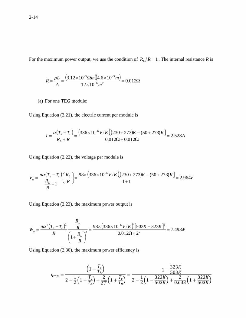
For the maximum power output, we use the condition of 1RRL . The internal resistance R is

012.01012

106.41012.326

35

m

mm

A

LR

(a) For one TEG module:

Using Equation (2.21), the electric current per module is

A

KKKV

RR

TTI

L

ch 528.2012.0012.0

)27350(27323010336 6

Using Equation (2.22), the voltage per module is

V

KKKV

R

R

R

R

TTnV L

L

chn 964.2

11

)27350(2732301033698

1

6

Using Equation (2.23), the maximum power output is

W

KKKV

R

R

R

R

R

TTnW

L

L

chn 493.7

2012.0

3235031033698

1

2

226

2

22

Using Equation (2.30), the maximum power efficiency is

𝜂𝑚𝑝 =(1 −

𝑇𝑐

𝑇ℎ)

2 −12 (1 −

𝑇𝑐

𝑇ℎ) +

2𝑍�̅�

(1 +𝑇𝑐

𝑇ℎ)

=1 −

323𝐾503𝐾

2 −12 (1 −

323𝐾503𝐾

) +2

0.633 (1 +323𝐾503𝐾

)

2-15

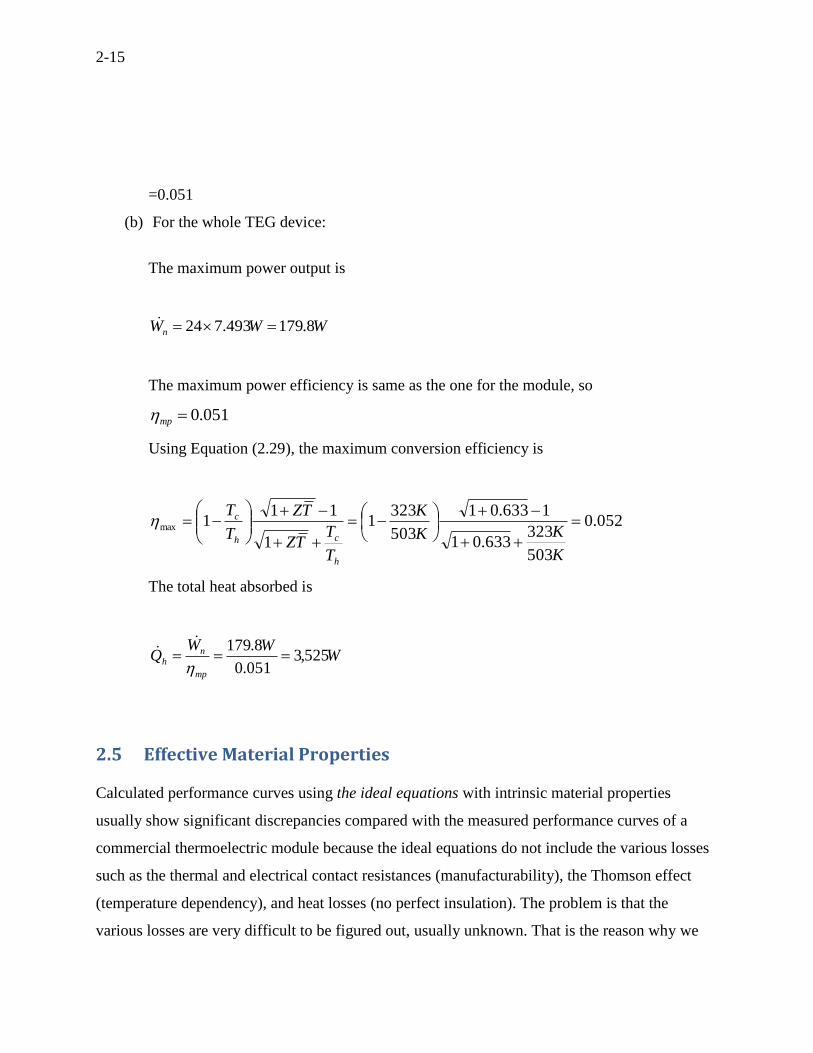
=0.051

(b) For the whole TEG device:

The maximum power output is

WWWn 8.179493.724

The maximum power efficiency is same as the one for the module, so

051.0mp

Using Equation (2.29), the maximum conversion efficiency is

052.0

503

323633.01

1633.01

503

3231

1

111max

K

KK

K

T

TTZ

TZ

T

T

h

ch

c

The total heat absorbed is

WWW

Qmp

nh 525,3

051.0

8.179

2.5 Effective Material Properties

Calculated performance curves using the ideal equations with intrinsic material properties

usually show significant discrepancies compared with the measured performance curves of a

commercial thermoelectric module because the ideal equations do not include the various losses

such as the thermal and electrical contact resistances (manufacturability), the Thomson effect

(temperature dependency), and heat losses (no perfect insulation). The problem is that the

various losses are very difficult to be figured out, usually unknown. That is the reason why we

2-16

developed the effective material properties to include those losses for a system design rather than

the intrinsic material properties. The following method shows how to determine the effective

material properties.

As mentioned before, the four maximum parameters are usually provided by manufacturers as

specification for a commercial module. However, the thermoelectric material properties (, , and

k) for the module are not usually provided by the manufacturers, which often causes a problem for

system designers who wants to simulate the module operation using the ideal equations. We have

four maximum parameters ( maxI , maxV , maxW , and mp ), which are ideally a function of three

material properties (, and k) with given geometry (A/L) of thermocouple and two junction

temperatures Th and Tc. Inversely, the three material properties can ideally be expressed from three

out of the four maximum parameters. It turned out that, the two parameters ( maxI and mp ) are

essential and any one of maxV and maxW can be used. We wish to deduce the three material

properties from the four manufactures’ maximum parameters. It is of interest to find that there

would be no convergence of the three material properties from the four measured maximum

parameters because of the contradiction of the ideal formulation and real measurements with

various energy losses. This enforces us to choose one of the two parameters ( maxV and maxW ) and

the essential two parameters ( maxI and mp ). We choose the maximum power output instead of the

maximum voltage because of the practical importance of power output. The effective material

properties are defined here as the realistic material properties that are extracted from the maximum

parameters provided by the manufacturers. So that the calculated effective material properties

include all kind of losses due to the thermal and electrical contact resistances, the temperature

dependence of the properties, and heat losses to ambient in addition to the intrinsic material

properties. This renders the dimensionless figure of merit for the effective material properties to

be slightly lower than that of the intrinsic material properties. The effective electrical resistivity is

obtained using Equations (2.26) and (2.28), which is

2-17

2max

max4

In

WLA

(2.35)

The effective Seebeck coefficient can be obtained using Equation (2.26) and (2.34), which is

ch TTnI

W

max

max4

(2.36)

The effective figure of merit is obtained from Equation (2.29), which is

𝑍∗ =1

�̅�[

(1 +

𝜂𝑚𝑎𝑥

𝜂𝑐

𝑇𝑐

𝑇ℎ

1 −𝜂𝑚𝑎𝑥

𝜂𝑐

)

2

− 1

]

(2.37)

where hcc TT1 which is the Carnot cycle efficiency. Alternatively, the effective figure of

merit may be obtained from Equation (2.30) in terms of mp as

𝑍∗ =

2�̅�

(1 +𝑇𝑐

𝑇ℎ)

𝜂𝑐 (1

𝜂𝑚𝑝+

12) − 2

(2.38)

The effective thermal conductivity with *Z which is usually obtained from Equations (2.37) is

now obtained

𝑘∗ =𝛼∗2

𝜌∗𝑍∗

(2.39)

The effective material properties now include various effects such as the contact resistances,

Thomson effect, and radiation and convection heat losses. Hence, the effective figure of merits in

Table 2.1 might be slightly smaller than the intrinsic figure of merit (not shown in the table).

2-18

Note that these effective properties should be divided by two due to p-type and n-type

thermoelements.

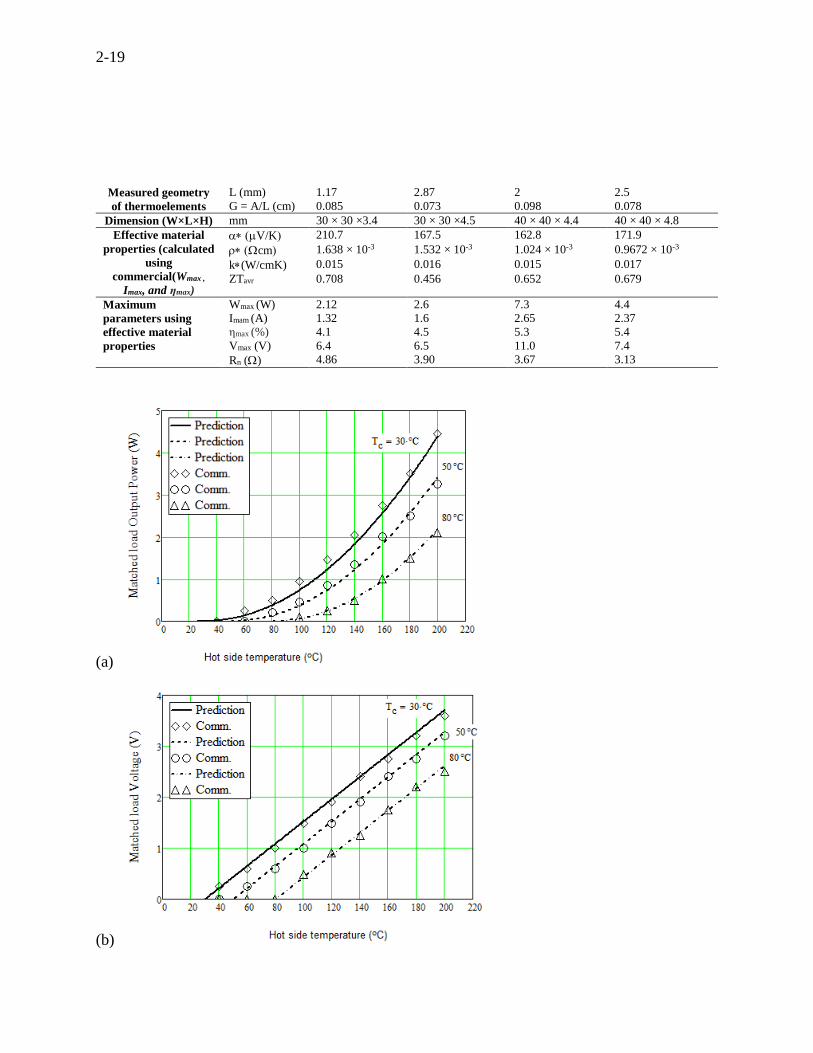
Comparison of calculations with a commercial product

The effective material properties can be calculated from any commercial thermoelectric

modules as long as the four maximum parameters are provided. Calculated effective material

properties from the maximum parameters for four selected commercial thermoelectric modules are

illustrated in Table 2.1. Then, we can simulate the performance curves of the module with these

effective material properties using the ideal equations. This is very useful for a system design with

thermoelectric modules. For example, we attained the effective material properties for TGM127-

1.4-2.5 module in Table 2.1 and compared the calculated performance curves with the performance

curves provided by the manufacturer, which are shown in Figure 2.1 (a) – (f). It is found that the

calculated results are in good agreement with the manufacturer’s performance curves (which are

typically experimental values).

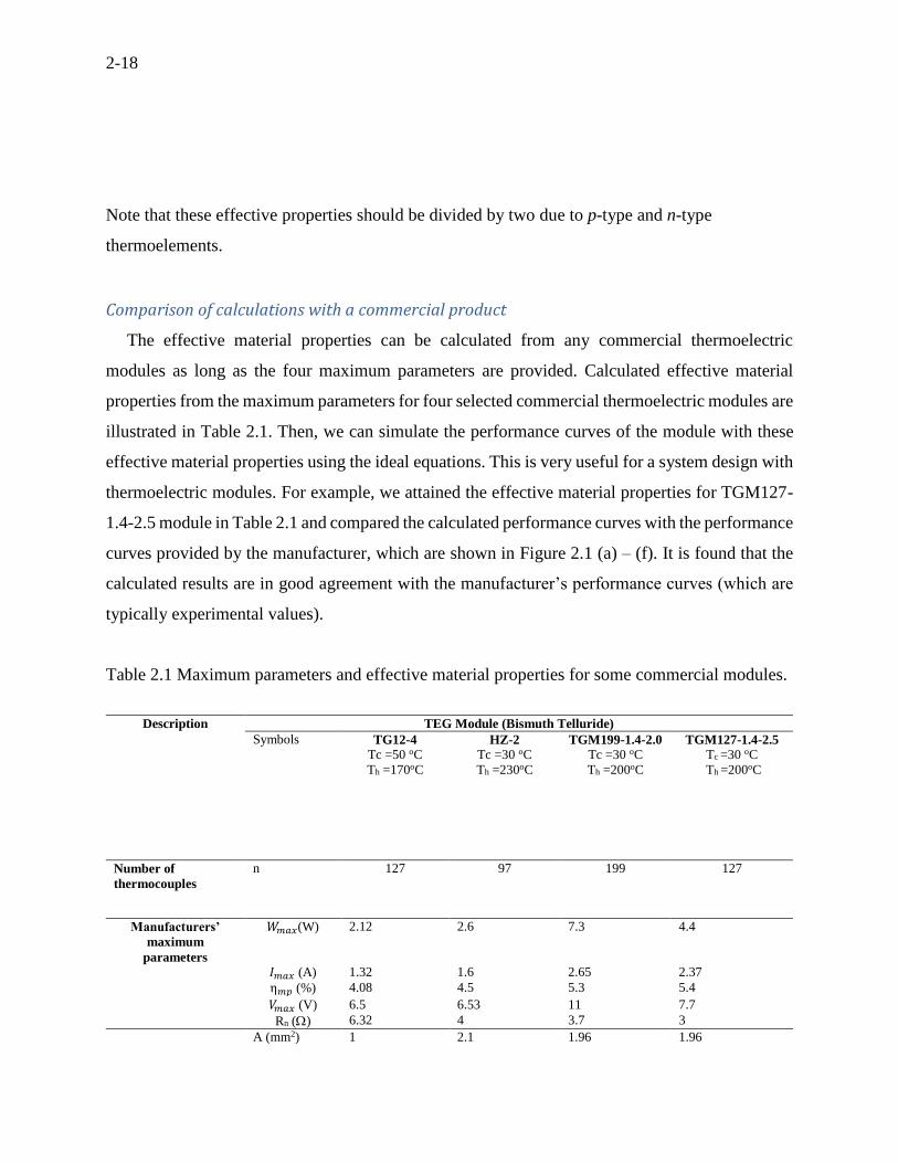
Table 2.1 Maximum parameters and effective material properties for some commercial modules.

Description TEG Module (Bismuth Telluride)

Symbols TG12-4

Tc =50 oC

Th =170oC

HZ-2

Tc =30 oC

Th =230oC

TGM199-1.4-2.0

Tc =30 oC

Th =200oC

TGM127-1.4-2.5

Tc =30 oC

Th =200oC

Number of

thermocouples

n 127 97 199 127

Manufacturers’

maximum

parameters

𝑊𝑚𝑎𝑥(W) 2.12 2.6 7.3 4.4

𝐼𝑚𝑎𝑥 (A) 1.32 1.6 2.65 2.37

η𝑚𝑝 (%) 4.08 4.5 5.3 5.4

𝑉𝑚𝑎𝑥 (V) 6.5 6.53 11 7.7

Rn () 6.32 4 3.7 3

A (mm2) 1 2.1 1.96 1.96

2-19

Measured geometry

of thermoelements

L (mm) 1.17 2.87 2 2.5

G = A/L (cm) 0.085 0.073 0.098 0.078

Dimension (W×L×H) mm 30 × 30 ×3.4 30 × 30 ×4.5 40 × 40 × 4.4 40 × 40 × 4.8

Effective material

properties (calculated

using

commercial(Wmax ,

Imax, and ηmax)

V/K 210.7 167.5 162.8 171.9

cm 1.638 × 10-3 1.532 × 10-3 1.024 × 10-3 0.9672 × 10-3

k(W/cmK) 0.015 0.016 0.015 0.017

ZTavr 0.708 0.456 0.652 0.679

Maximum

parameters using

effective material

properties

Wmax (W) 2.12 2.6 7.3 4.4

Imam (A) 1.32 1.6 2.65 2.37

ηmax (%) 4.1 4.5 5.3 5.4

Vmax (V) 6.4 6.5 11.0 7.4

Rn () 4.86 3.90 3.67 3.13

(a)

(b)

2-20

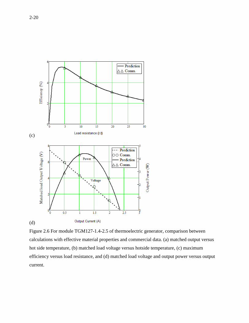
(c)

(d)

Figure 2.6 For module TGM127-1.4-2.5 of thermoelectric generator, comparison between

calculations with effective material properties and commercial data. (a) matched output versus

hot side temperature, (b) matched load voltage versus hotside temperature, (c) maximum

efficiency versus load resistance, and (d) matched load voltage and output power versus output

current.

2-21

Problems

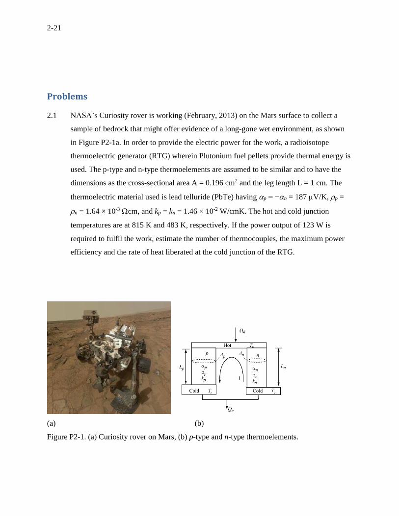
2.1 NASA’s Curiosity rover is working (February, 2013) on the Mars surface to collect a

sample of bedrock that might offer evidence of a long-gone wet environment, as shown

in Figure P2-1a. In order to provide the electric power for the work, a radioisotope

thermoelectric generator (RTG) wherein Plutonium fuel pellets provide thermal energy is

used. The p-type and n-type thermoelements are assumed to be similar and to have the

dimensions as the cross-sectional area A = 0.196 cm2 and the leg length L = 1 cm. The

thermoelectric material used is lead telluride (PbTe) having p = −n = 187 V/K, p =

n = 1.64 × 10-3 cm, and kp = kn = 1.46 × 10-2 W/cmK. The hot and cold junction

temperatures are at 815 K and 483 K, respectively. If the power output of 123 W is

required to fulfil the work, estimate the number of thermocouples, the maximum power

efficiency and the rate of heat liberated at the cold junction of the RTG.

(a) (b)

Figure P2-1. (a) Curiosity rover on Mars, (b) p-type and n-type thermoelements.

2-22

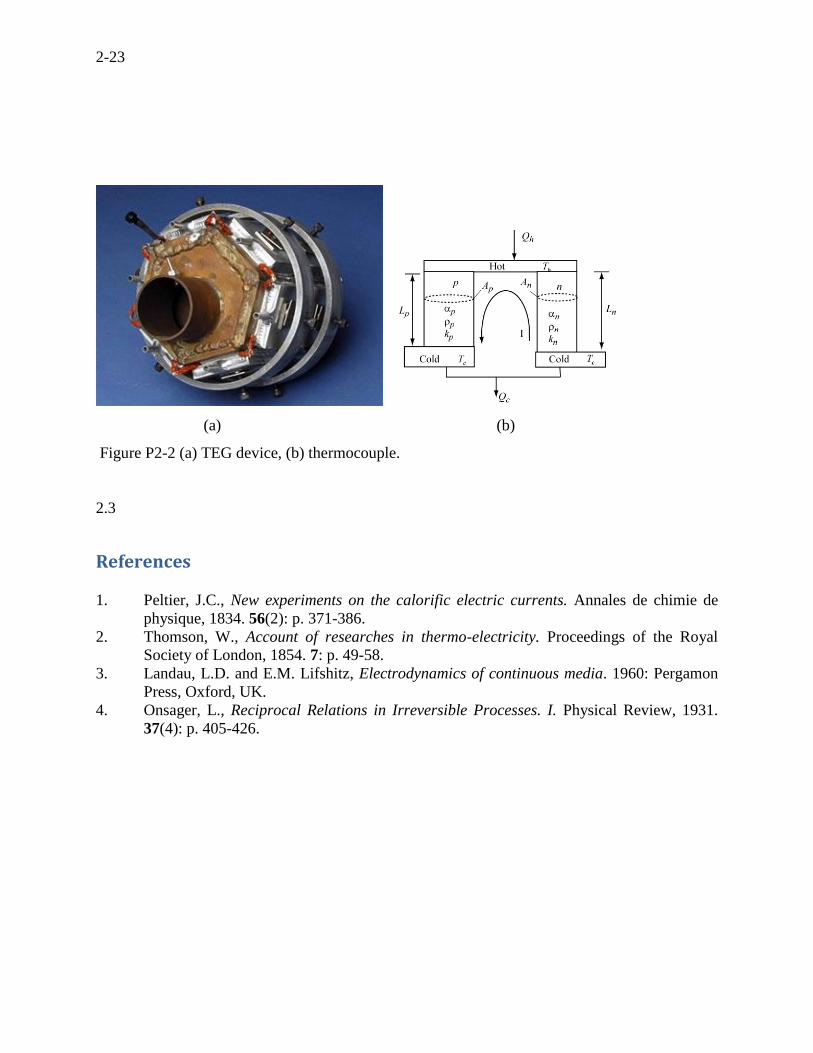
2.2 We want to recover waste heat from the exhaust gas of a car using thermoelectric

generator (TEG) modules as shown in Figure P2-2. An array of N = 36 TEG modules is

installed on the exhaust of the car. Each module has n = 127 thermocouples that consist

of p-type and n-type thermoelements. Exhaust gases flow through the TEG device,

wherein one side of the modules experiences the exhaust gases while the other side of the

modules experiences coolant flows. These cause the hot and cold junction temperatures

of the modules to be at 230 °C and 50 °C, respectively. To maintain the junction

temperatures, the significant amount of heat should be absorbed at the hot junction and

liberated at the cold junction, which usually achieved by heat sinks. The material

properties for the p-type and n-type thermoelements are assumed to be similar. The most

appropriate module of TG12-4 for this work found in the commercial products shows the

maximum parameters rather than the material properties as the number of couples of 127,

the maximum power of 4.05 W, the short circuit current of 1.71 A, the maximum

efficiency of 4.97 %, and the open circuit voltage of 9.45 V. The cross-sectional area and

leg length of the thermoelements are An = Ap = 1.0 mm2 and Ln = Lp = 1.17 mm,

respectively, which are shown in Figure P-1b.

(a) Estimate the effective material properties: the Seebeck coefficient, the electrical

resistivity, and the thermal conductivity.

(b) Per one TEG module, compute the electric current, the voltage, the maximum

power output, and the maximum power efficiency.

(c) For the whole TEG device, compute the maximum power output, the maximum

power efficiency, the maximum conversion efficiency and the total heat absorbed at

the hot junction.

2-23

(a) (b)

Figure P2-2 (a) TEG device, (b) thermocouple.

2.3

References

1. Peltier, J.C., New experiments on the calorific electric currents. Annales de chimie de

physique, 1834. 56(2): p. 371-386.

2. Thomson, W., Account of researches in thermo-electricity. Proceedings of the Royal

Society of London, 1854. 7: p. 49-58.

3. Landau, L.D. and E.M. Lifshitz, Electrodynamics of continuous media. 1960: Pergamon

Press, Oxford, UK.

4. Onsager, L., Reciprocal Relations in Irreversible Processes. I. Physical Review, 1931.

37(4): p. 405-426.