Embed Size (px)
Citation preview
3-1
Chapter 3 Thermoelectric
Coolers This chapter formulates the simplified ideal equations for a thermoelectric cooler with some
assumptions to see the general characteristics of thermoelectric coolers. The maximum parameters
are defined, which are the maximum current, maximum temperature difference, maximum cooling
power, and maximum voltage. Then, the normalized parameters are plotted as general
characteristics for the coolers. The ideal equation is based on three material properties, which are
the Seebeck coefficient, electrical resistivity, and thermal conductivity. These material properties
for commercial thermoelectric cooler modules are not usually provided by the manufacturers as
their proprietary information but the maximum properties. Therefore, the effective material
properties are developed from the available maximum parameters of the product with fair
agreement with the measurements. These are used for prediction of performance and design later.
3.1 Ideal Equations
Since the discovery of thermoelectric effects in the early nineteenth century, a very essential
equation for the rate of heat flow per unit area �⃗� was formulated as shown in Equation (2.3),
which is
q⃗⃗ = 𝛼𝑇𝑗 − 𝑘∇⃗⃗⃗T (3.1)
3-2
where is the Seebeck coefficient, 𝑗 the current density, k the thermal conductivity and ∇⃗⃗⃗ the
gradient. This equation relates the heat flow, the electric current and the thermal conduction,
leading to the steady-state heat diffusion equation as shown in Equation (2.7), which is rewritten
here as
02 TjdT
dTjTk
(3.2)
where is the electrical resistivity. The first term gives the thermal conduction, the second term
gives the Joule heating, and the third term pertains to the Thomson effect which results from the
temperature-dependent Seebeck coefficient. The above two equation governs the thermoelectric
phenomena.
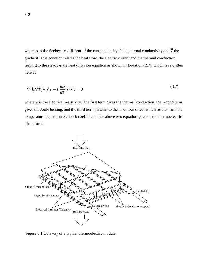
Figure 3.1 Cutaway of a typical thermoelectric module
p
n
p
n
np
p
pn
Positive (+)
Negative (-)
Heat Absorbed
Heat Rejected
Electrical Conductor (copper)Electrical Insulator (Ceramic)
p-type Semiconcuctor
n-type Semiconductor
3-3
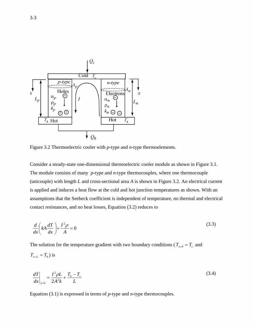
Figure 3.2 Thermoelectric cooler with p-type and n-type thermoelements.
Consider a steady-state one-dimensional thermoelectric cooler module as shown in Figure 3.1.
The module consists of many p-type and n-type thermocouples, where one thermocouple
(unicouple) with length L and cross-sectional area A is shown in Figure 3.2. An electrical current
is applied and induces a heat flow at the cold and hot junction temperatures as shown. With an
assumptions that the Seebeck coefficient is independent of temperature, no thermal and electrical
contact resistances, and no heat losses, Equation (3.2) reduces to
02
A
I
dx
dTkA
dx
d
(3.3)
The solution for the temperature gradient with two boundary conditions ( cx TT 0 and
hLx TT ) is
L
TT
kA
LI
dx
dT ch
x
2
2
0 2
(3.4)
Equation (3.1) is expressed in terms of p-type and n-type thermocouples.
3-4
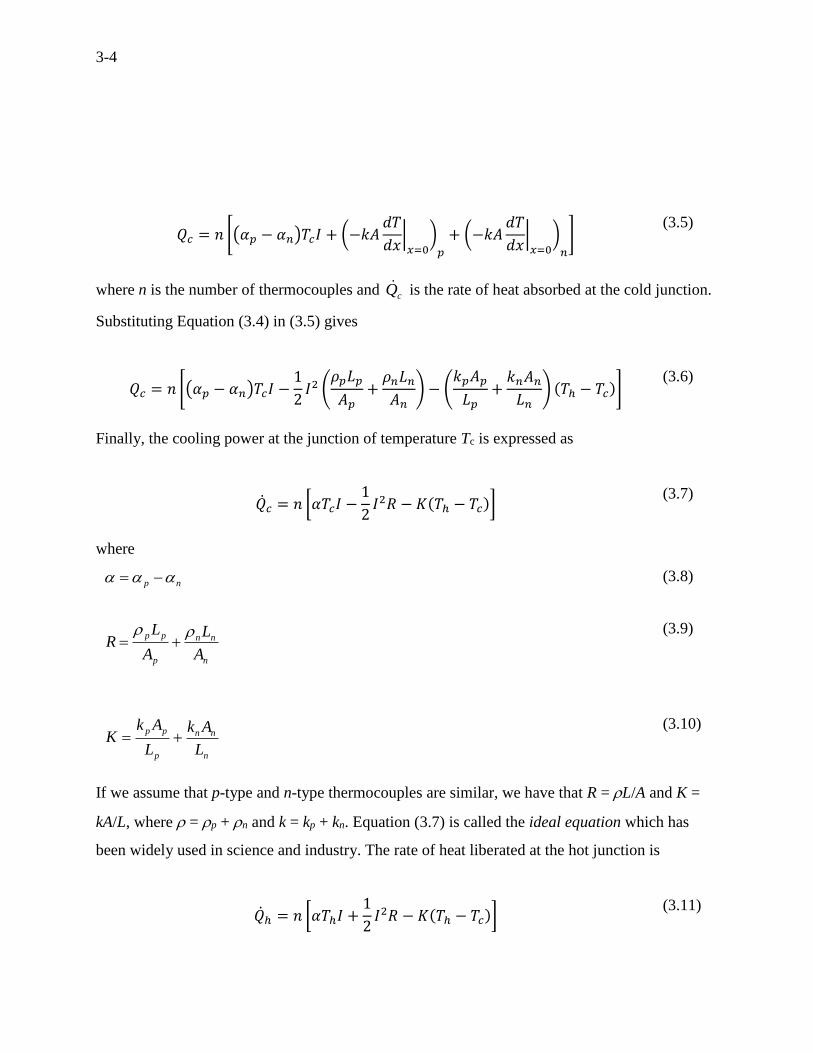
𝑄𝑐 = 𝑛 [(𝛼𝑝 − 𝛼𝑛)𝑇𝑐𝐼 + (−𝑘𝐴𝑑𝑇
𝑑𝑥|𝑥=0
)𝑝
+ (−𝑘𝐴𝑑𝑇
𝑑𝑥|𝑥=0
)𝑛
] (3.5)
where n is the number of thermocouples and cQ is the rate of heat absorbed at the cold junction.
Substituting Equation (3.4) in (3.5) gives
𝑄𝑐 = 𝑛 [(𝛼𝑝 − 𝛼𝑛)𝑇𝑐𝐼 −1
2𝐼2 (
𝜌𝑝𝐿𝑝
𝐴𝑝+𝜌𝑛𝐿𝑛𝐴𝑛
) − (𝑘𝑝𝐴𝑝
𝐿𝑝+𝑘𝑛𝐴𝑛
𝐿𝑛) (𝑇ℎ − 𝑇𝑐)]
(3.6)
Finally, the cooling power at the junction of temperature Tc is expressed as
�̇�𝑐 = 𝑛 [𝛼𝑇𝑐𝐼 −1
2𝐼2𝑅 − 𝐾(𝑇ℎ − 𝑇𝑐)]
(3.7)
where
np (3.8)
n
nn
p
pp
A
L
A
LR
(3.9)
n
nn
p
pp
L
Ak
L
AkK
(3.10)
If we assume that p-type and n-type thermocouples are similar, we have that R = L/A and K =
kA/L, where = p + n and k = kp + kn. Equation (3.7) is called the ideal equation which has
been widely used in science and industry. The rate of heat liberated at the hot junction is
�̇�ℎ = 𝑛 [𝛼𝑇ℎ𝐼 +1
2𝐼2𝑅 − 𝐾(𝑇ℎ − 𝑇𝑐)]
(3.11)
3-5
Considering the 1st law of thermodynamics across the thermoelectric device, we have
�̇� = �̇�ℎ − �̇�𝑐 (3.12)
The amount of work per unit time across the module (rate of work) is obtained substituting
Equations (3.7) and (3.11) in (3.12).
�̇� = 𝑛[𝛼𝐼(𝑇ℎ − 𝑇𝑐) + 𝐼2𝑅] (3.13)
where the first term is the rate of work to overcome the thermoelectric voltage, whereas the
second term is the resistive loss. Since the power is IVW , the voltage across the couple will
be
𝑉 = 𝑛[𝛼(𝑇ℎ − 𝑇𝑐) + 𝐼𝑅] (3.14)
The COP is defined by the ratio of the cooling power to the input electrical power.
𝐶𝑂𝑃 =�̇�𝑐
�̇�=𝑛 [𝛼𝑇𝑐𝐼 −
12𝐼2𝑅 − 𝐾(𝑇ℎ − 𝑇𝑐)]
𝑛[𝛼𝐼(𝑇ℎ − 𝑇𝑐) + 𝐼2𝑅]
(3.15)
There are two values of the current that are of special interest: the current Imp that yields the
maximum cooling power and the current ICOP that yields the maximum COP. The maximum
cooling power can be obtained by differentiating Equation (3.7) and setting it to zero. The
current for the maximum cooling power is found to be
R
TI c
mp
(3.16)
3-6
The optimum COP can be obtained by differentiating Equation (3.15) and setting it to zero
𝑑(𝐶𝑂𝑃)
𝑑𝐼= 0
(3.17)
We finally have
11
TZR
TICOP
(3.18)
where ∆𝑇 = 𝑇ℎ − 𝑇𝑐, kZ 2 and T is the average temperature of cT and hT . On the basis of
Th, TZ is expressed by
h
hT
TZTTZ
21
(3.19)
3.2 Maximum Parameters
Let us consider a thermoelectric module shown in Figure 3.1 for the theoretical maximum
parameters with the ideal equation. The module consists of a number of thermocouples as shown.
The ideal equation assumes that there are no the electrical and thermal contact resistances, no
Thomson effect, and no radiation or convection. It is noted that the theoretical maximum
parameters might differ with the manufacturers’ maximum parameters that are usually obtained
through measurements.
The maximum current Imax is the current that produces the maximum possible temperature
difference Tmax , which always occurs when the cooling power is at zero. This is obtained by
setting cQ = 0 in Equation (3.7), replacing Tc with (Th – T) and taking derivative of T with
respect to I and setting it to zero. The maximum current is finally expressed by
3-7
ZT
ZT
RI hh
11 2
2
max
(3.20)
Or, equivalently in terms of Tmax,
R
TTI h max
max
(3.21)
The maximum temperature difference Tmax is the maximum possible temperature difference
Tmax , which always occurs when the cooling power is at zero and the current is at maximum.
This is obtained by setting cQ = 0 in Equation (3.7), substituting both I and Tc by Imax and Th –
Tmax, respectively, and solving for Tmax. The maximum temperature difference is obtained as
2
2
max
11hhh T
ZT
ZTT
(3.22)
where the figure of merit Z (unit: K-1) is given by
kZ
2
or RK
Z2
(3.23)
The maximum cooling power maxcQ is the maximum thermal load which occurs at T = 0 and I
= Imax. This can be obtained by substituting both I and Tc in Equation (3.7) by Imax and Th,
respectively, and solving for maxcQ . The maximum cooling power for a thermoelectric module
with n thermocouples is
R
TTnQ h
c2
2
max
22
max
(3.24)
3-8
The maximum voltage is the DC voltage which delivers the maximum possible temperature
difference Tmax when I = Imax. The maximum voltage is obtained from Equation (3.14), which is
hTnV max (3.25)
3.3 Normalized Parameters
If we divide the active values by the maximum values, we can normalize the characteristics of
the thermoelectric cooler. The normalized cooling power can be obtained by dividing Equation
(3.7) by Equation (3.24), which is
RTTn
TKRIITTn
Q
Q
h
h
c
c
2
2
1
2
max
22
2
max
(3.26)
which, in terms of the normalized current and normalized temperature difference, reduces to
2
max
max
max
max
2
max
max
max
max
max
max
max
1
2
1
1
1
12
h
h
h
h
h
h
h
c
c
T
TZT
T
T
T
T
T
T
I
I
T
T
T
T
I
I
T
T
T
T
Q
Q
(3.27)
where
11
11
1
2
max
hhh ZTZTT
T
(3.28)
The coefficient of performance in terms of the normalized values is
3-9
2
max
max
max
max
max
max
max
max
2
max
max
max
max
max
1
1
12
11
I
I
T
T
I
I
T
T
T
T
T
TZT
T
T
T
T
I
I
T
T
I
I
T
T
T
T
COP
hh
h
h
h
hh
(3.29)
The normalized voltage is
max
maxmax
maxmax
1I
I
T
T
T
T
T
T
V
V
hh
(3.30)
The normalized current for the optimum COP is obtained from Equation (3.18).
111 max
max
max
max
TZT
T
T
T
T
T
I
I
h
hCOP
(3.31)
where TZ is expressed using Equation (3.19) and Equation (3.28) by
max
max
2
11
T
T
T
TZTTZ
h
h (3.32)
Note that the above normalized values in Equations (3.27), (3.29) and (3.30) are a function of three
parameters, which are maxTT , maxII and ZTh. Figure 3.3 and Figure 3.4 are based on the ideal
equations using the normalized parameters. The three maximum parameters of Tmax, Imax, and
maxcQ are predictable inversely with the effective material properties, we can then use the
normalized charts for estimation of the performance. The solid lines for the both figures indicate
the normalized prediction with ZTh = 0.75 which is approximately an average commercial value
(see Table 3.2).
3-10
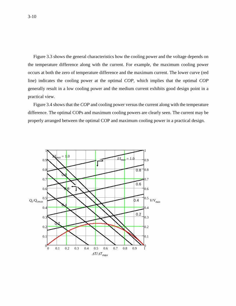
Figure 3.3 shows the general characteristics how the cooling power and the voltage depends on
the temperature difference along with the current. For example, the maximum cooling power
occurs at both the zero of temperature difference and the maximum current. The lower curve (red
line) indicates the cooling power at the optimal COP, which implies that the optimal COP
generally result in a low cooling power and the medium current exhibits good design point in a
practical view.
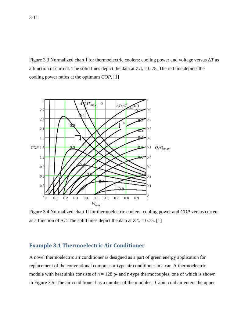
Figure 3.4 shows that the COP and cooling power versus the current along with the temperature
difference. The optimal COPs and maximum cooling powers are clearly seen. The current may be
properly arranged between the optimal COP and maximum cooling power in a practical design.
0 0.1 0.2 0.3 0.4 0.5 0.6 0.7 0.8 0.9 10
0.1
0.2
0.3
0.4
0.5
0.6
0.7
0.8
0.9
1
0
0.1
0.2
0.3
0.4
0.5
0.6
0.7
0.8
0.9
1
I/Imax = 1.0I/Imax = 1.0
0.8
0.8
0.6
0.6
Qc/Qcmax 0.4 V/Vmax
0.4
0.2
0.2
T/Tmax
3-11
Figure 3.3 Normalized chart I for thermoelectric coolers: cooling power and voltage versus T as
a function of current. The solid lines depict the data at ZTh = 0.75. The red line depicts the
cooling power ratios at the optimum COP. [1]
Figure 3.4 Normalized chart II for thermoelectric coolers: cooling power and COP versus current
as a function of T. The solid lines depict the data at ZTh = 0.75. [1]
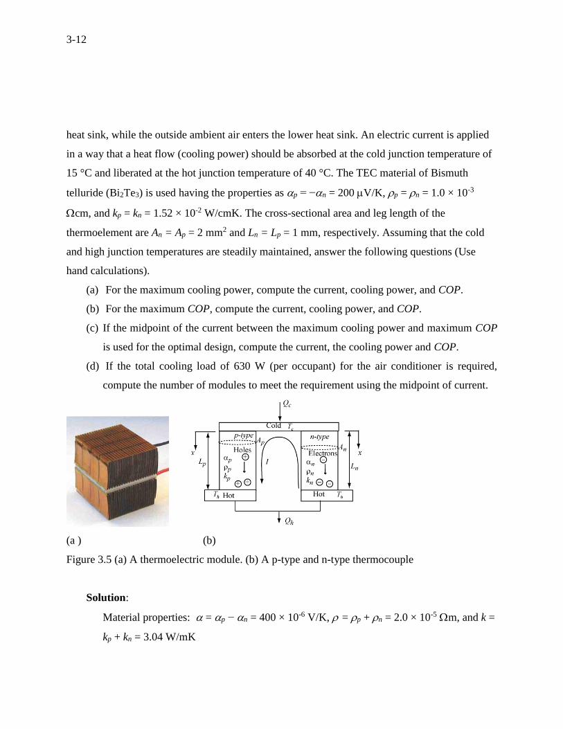
Example 3.1 Thermoelectric Air Conditioner
A novel thermoelectric air conditioner is designed as a part of green energy application for
replacement of the conventional compressor-type air conditioner in a car. A thermoelectric
module with heat sinks consists of n = 128 p- and n-type thermocouples, one of which is shown
in Figure 3.5. The air conditioner has a number of the modules. Cabin cold air enters the upper
0 0.1 0.2 0.3 0.4 0.5 0.6 0.7 0.8 0.9 10
0.3
0.6
0.9
1.2
1.5
1.8
2.1
2.4
2.7
3
0
0.1
0.2
0.3
0.4
0.5
0.6
0.7
0.8
0.9
1T/Tmax = 0
T/Tmax = 0
0.1
0.1
0.2
0.2
0.3
0.4
COP 0.3 0.5 Qc/Qcmax
0.6
0.4
0.5 0.8
0.6
0.8
I/Imax
3-12
heat sink, while the outside ambient air enters the lower heat sink. An electric current is applied
in a way that a heat flow (cooling power) should be absorbed at the cold junction temperature of
15 °C and liberated at the hot junction temperature of 40 °C. The TEC material of Bismuth
telluride (Bi2Te3) is used having the properties as p = −n = 200 V/K, p = n = 1.0 × 10⁻³
cm, and kp = kn = 1.52 × 10⁻² W/cmK. The cross-sectional area and leg length of the
thermoelement are An = Ap = 2 mm2 and Ln = Lp = 1 mm, respectively. Assuming that the cold
and high junction temperatures are steadily maintained, answer the following questions (Use
hand calculations).
(a) For the maximum cooling power, compute the current, cooling power, and COP.
(b) For the maximum COP, compute the current, cooling power, and COP.
(c) If the midpoint of the current between the maximum cooling power and maximum COP
is used for the optimal design, compute the current, the cooling power and COP.
(d) If the total cooling load of 630 W (per occupant) for the air conditioner is required,
compute the number of modules to meet the requirement using the midpoint of current.
(a ) (b)
Figure 3.5 (a) A thermoelectric module. (b) A p-type and n-type thermocouple
Solution:
Material properties: =p − n = 400 × 10-6 V/K, = p + n = 2.0 × 10⁻⁵ m, and k =
kp + kn = 3.04 W/mK
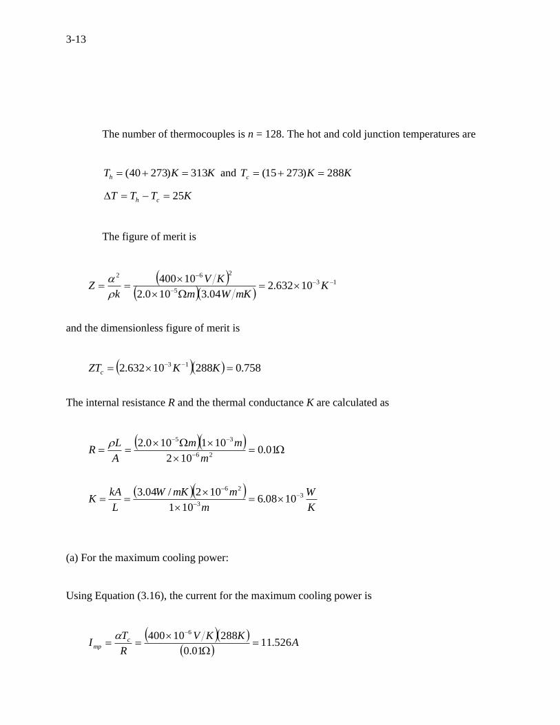
3-13
The number of thermocouples is n = 128. The hot and cold junction temperatures are
KKTh 313)27340( and KKTc 288)27315(
KTTT ch 25
The figure of merit is
13
5
262
10632.204.3100.2
10400
K
mKWm
KV
kZ
and the dimensionless figure of merit is
758.028810632.2 13 KKZTc
The internal resistance R and the thermal conductance K are calculated as
01.0102
101100.226
35
m
mm
A
LR
K
W
m
mmKW
L
kAK 3
3
26
1008.6101
102/04.3
(a) For the maximum cooling power:
Using Equation (3.16), the current for the maximum cooling power is
AKKV
R
TI c
mp 526.1101.0
28810400 6

3-14
Using Equation (3.7), the maximum cooling power is
W
KK
WAAKKV
TKRIITnQ mpmpccmp
567.65
251008.601.0526.112
1526.1128810400128
2
1
326
2
Using Equation (3.13), the power input is
WAKAKV
RITTInW mpchmpnmp
8.18401.0526.1125526.111040012826
2
Using Equation (3.15), the COP at the maximum cooling power is
355.08.184
567.65
W
W
W
QCOP
nmp
cmp
mp
(b) For the maximum COP:
791.02
2510632.2
2
13
KK
TTZTZ ch
Using Equation (3.18), the current for the maximum COP is
AKKV
TZR
TICOP 956.2
1791.0101.0
2510400
11
6
Using Equation (3.7), the maximum cooling power is
3-15
W
KK
WAAKKV
TKRIITnQ copcopcncop
557.18
251008.601.0956.22
1956.228810400128
2
1
326
2
Using Equation (3.13), the maximum power input is
WAKAKV
RITTInW copchcopncop
964.1401.0956.225956.21040012826
2
Using Equation (3.15), the COP is
24.1964.14
557.18max
W
W
W
QCOP
ncop
ncop
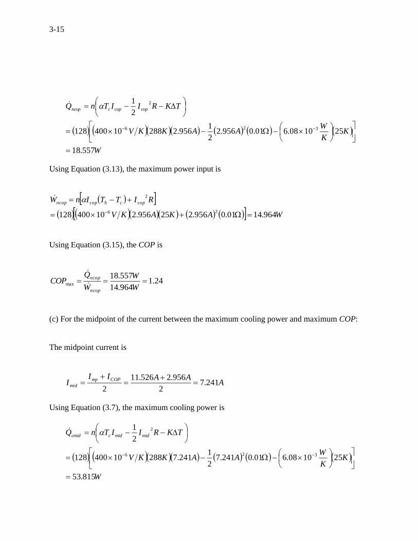
(c) For the midpoint of the current between the maximum cooling power and maximum COP:
The midpoint current is
AAAII
ICOPmp
mid 241.72
956.2526.11
2
Using Equation (3.7), the maximum cooling power is
W
KK
WAAKKV
TKRIITnQ midmidccmid
815.53
251008.601.0241.72
1241.728810400128
2
1
326
2
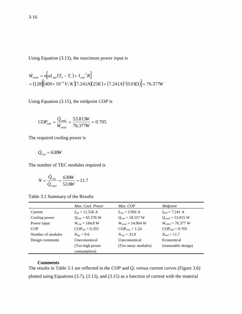
3-16
Using Equation (3.13), the maximum power input is
WAKAKV
RITTInW midchmidnmid
377.7601.0241.725241.71040012826
2
Using Equation (3.15), the midpoint COP is
705.0377.76
815.53
W
W
W
QCOP
nmid
cmidmid
The required cooling power is
WQreq 630
The number of TEC modules required is
7.118.53
630
W
W
Q
QN
cmid
req
Table 3.1 Summary of the Results
Max. Cool. Power Max. COP Midpoint
Current Imp = 11.526 A Icop = 2.956 A Imid = 7.241 A
Cooling power Qcmp = 65.576 W Qcop = 18.557 W Qcmid = 53.815 W
Power input Wcnp = 184.8 W Wncop = 14.964 W Wnmid = 76.377 W
COP COPmp = 0.355 COPmax = 1.24 COPmid = 0.705
Number of modules Nmp = 9.6 Ncop = 33.9 Nmid = 11.7
Design comments Uneconomical
(Too high power
consumption)
Uneconomical
(Too many modules)
Economical
(reasonable design)
Comments
The results in Table 3.1 are reflected in the COP and Qc versus current curves (Figure 3.6)
plotted using Equations (3.7), (3.13), and (3.15) as a function of current with the material
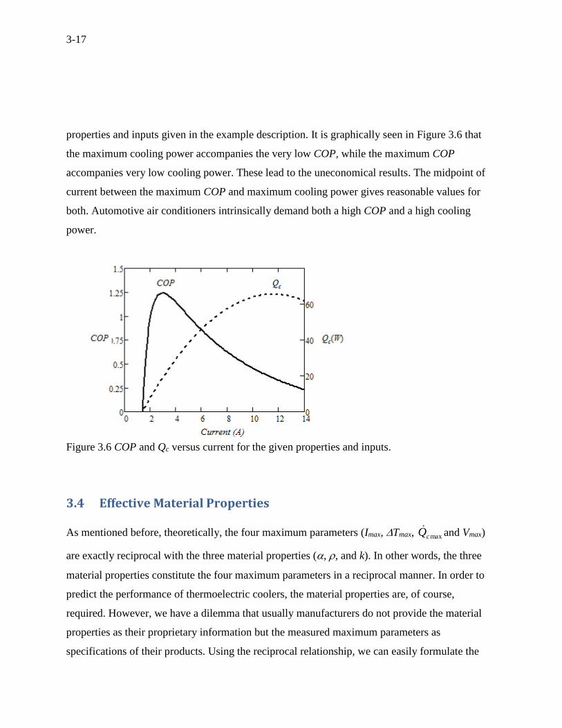
3-17
properties and inputs given in the example description. It is graphically seen in Figure 3.6 that
the maximum cooling power accompanies the very low COP, while the maximum COP
accompanies very low cooling power. These lead to the uneconomical results. The midpoint of
current between the maximum COP and maximum cooling power gives reasonable values for
both. Automotive air conditioners intrinsically demand both a high COP and a high cooling
power.
Figure 3.6 COP and Qc versus current for the given properties and inputs.
3.4 Effective Material Properties
As mentioned before, theoretically, the four maximum parameters (Imax, Tmax, maxcQ and Vmax)
are exactly reciprocal with the three material properties (, , and k). In other words, the three
material properties constitute the four maximum parameters in a reciprocal manner. In order to
predict the performance of thermoelectric coolers, the material properties are, of course,
required. However, we have a dilemma that usually manufacturers do not provide the material
properties as their proprietary information but the measured maximum parameters as
specifications of their products. Using the reciprocal relationship, we can easily formulate the
3-18
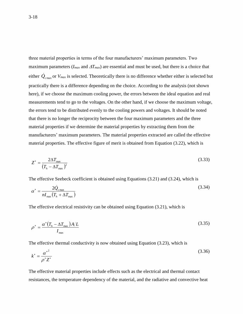
three material properties in terms of the four manufacturers’ maximum parameters. Two
maximum parameters (Imax and Tmax) are essential and must be used, but there is a choice that
either maxcQ or Vmax is selected. Theoretically there is no difference whether either is selected but
practically there is a difference depending on the choice. According to the analysis (not shown
here), if we choose the maximum cooling power, the errors between the ideal equation and real
measurements tend to go to the voltages. On the other hand, if we choose the maximum voltage,
the errors tend to be distributed evenly to the cooling powers and voltages. It should be noted
that there is no longer the reciprocity between the four maximum parameters and the three
material properties if we determine the material properties by extracting them from the
manufacturers’ maximum parameters. The material properties extracted are called the effective
material properties. The effective figure of merit is obtained from Equation (3.22), which is
2max
max2
TT
TZ
h
(3.33)
The effective Seebeck coefficient is obtained using Equations (3.21) and (3.24), which is
maxmax
max2
TTnI
Q
h
c
(3.34)
The effective electrical resistivity can be obtained using Equation (3.21), which is
max
max
I
LATTh
(3.35)
The effective thermal conductivity is now obtained using Equation (3.23), which is
Zk
2
(3.36)
The effective material properties include effects such as the electrical and thermal contact
resistances, the temperature dependency of the material, and the radiative and convective heat
3-19
losses. Hence, the effective figure of merit appears slightly smaller than the intrinsic figure of
merit as shown in Table 1. Since the material properties were obtained for a p-type and n-type
thermocouple, the material properties of a thermoelement (either p-type or n-type) should be
attained by dividing it by 2.
Comparison of Calculations with a Commercial Product
The effective material properties can be calculated from any commercial thermoelectric module
modules as long as the four maximum parameters are provided. Calculated effective material
properties from the maximum parameters for four commercial thermoelectric modules are
illustrated in Table 3.2. Then, we can simulate the performance curves of the module with these
effective material properties using the ideal equations. For example, we obtained the effective
material properties for C2-30-1503 module in Table 3.2 and compared the calculated
performance curves with the commercial performance curves, which are shown in Figure 3.7(a)
–(c). It is found that the calculated results are in good agreement with the manufacturer’s curves
(which are typically experimental values)
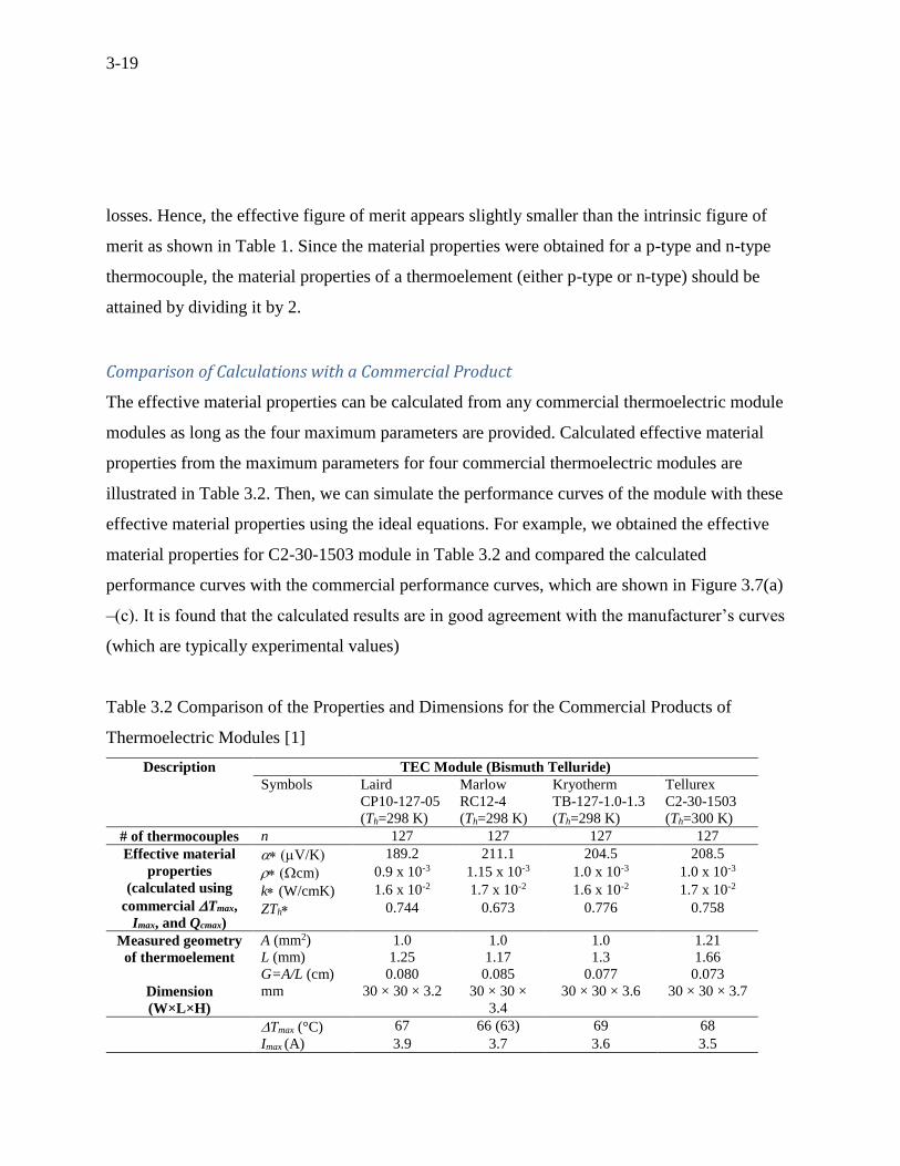
Table 3.2 Comparison of the Properties and Dimensions for the Commercial Products of
Thermoelectric Modules [1]
Description TEC Module (Bismuth Telluride)
Symbols Laird
CP10-127-05
(Th=298 K)
Marlow
RC12-4
(Th=298 K)
Kryotherm
TB-127-1.0-1.3
(Th=298 K)
Tellurex
C2-30-1503
(Th=300 K)
# of thermocouples n 127 127 127 127
Effective material
properties
(calculated using
commercial Tmax,
Imax, and Qcmax)
V/K 189.2 211.1 204.5 208.5
cm 0.9 x 10⁻³ 1.15 x 10⁻³ 1.0 x 10⁻³ 1.0 x 10⁻³
k (W/cmK) 1.6 x 10⁻² 1.7 x 10⁻² 1.6 x 10⁻² 1.7 x 10⁻²
ZTh 0.744 0.673 0.776 0.758
Measured geometry
of thermoelement
A (mm2) 1.0 1.0 1.0 1.21
L (mm) 1.25 1.17 1.3 1.66
G=A/L (cm) 0.080 0.085 0.077 0.073
Dimension
(W×L×H)
mm 30 × 30 × 3.2 30 × 30 ×
3.4
30 × 30 × 3.6 30 × 30 × 3.7
Tmax (°C) 67 66 (63) 69 68
Imax (A) 3.9 3.7 3.6 3.5
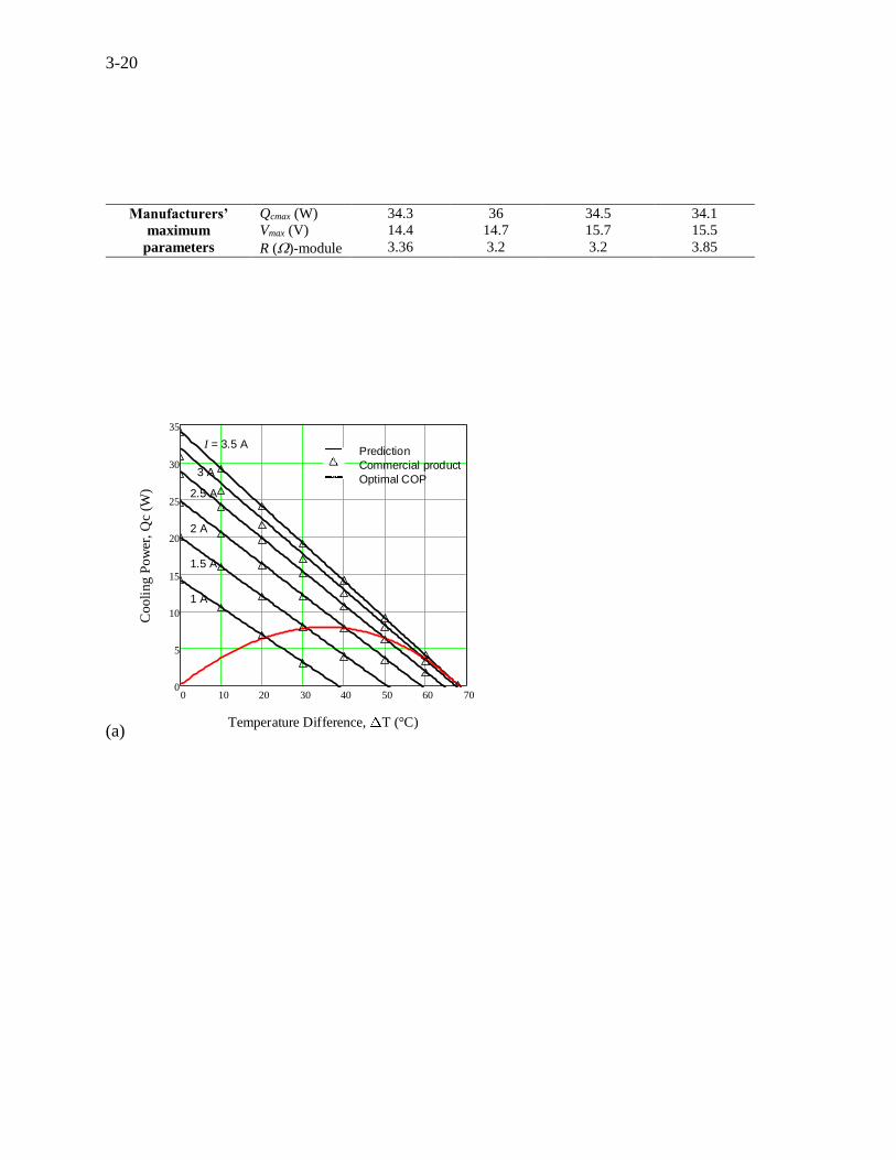
3-20
Manufacturers’
maximum
parameters
Qcmax (W) 34.3 36 34.5 34.1
Vmax (V) 14.4 14.7 15.7 15.5
R ()-module 3.36 3.2 3.2 3.85
(a)
0 10 20 30 40 50 60 700
5
10
15
20
25
30
35
Temperature Difference, T (°C)
Cooli
ng P
ow
er, Q
c (W
)
I = 3.5 APrediction
Commercial product3 A
Optimal COP
2.5 A
2 A
1.5 A
1 A
3-21
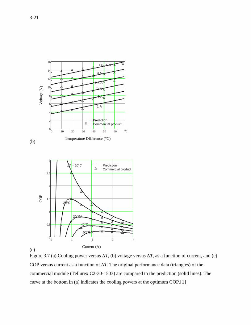
(b)
(c)
Figure 3.7 (a) Cooling power versus T, (b) voltage versus T, as a function of current, and (c)
COP versus current as a function of T. The original performance data (triangles) of the
commercial module (Tellurex C2-30-1503) are compared to the prediction (solid lines). The
curve at the bottom in (a) indicates the cooling powers at the optimum COP.[1]
0 10 20 30 40 50 60 700
2
4
6
8
10
12
14
16
Temperature Difference (°C)
Vol
tage
(V)
I = 3.5 A
3 A
2.5 A
2 A
1.5 A
1 A
Prediction
Commercial product
0 1 2 3 40
0.5
1
1.5
2
2.5
3
Current (A)
CO
P
T = 10°C Prediction
Commercial product
20°C
30°C
40°C
50°C
3-22
Problems
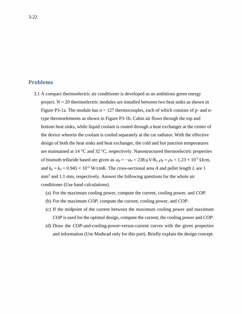
3.1 A compact thermoelectric air conditioner is developed as an ambitious green energy
project. N = 20 thermoelectric modules are installed between two heat sinks as shown in
Figure P3-1a. The module has n = 127 thermocouples, each of which consists of p- and n-
type thermoelements as shown in Figure P3-1b. Cabin air flows through the top and
bottom heat sinks, while liquid coolant is routed through a heat exchanger at the center of
the device wherein the coolant is cooled separately at the car radiator. With the effective
design of both the heat sinks and heat exchanger, the cold and hot junction temperatures
are maintained at 14 °C and 32 °C, respectively. Nanostructured thermoelectric properties
of bismuth telluride based are given as p = −n = 238 V/K, p = n = 1.23 × 10⁻³ cm,
and kp = kn = 0.945 × 10⁻² W/cmK. The cross-sectional area A and pellet length L are 1
mm2 and 1.1 mm, respectively. Answer the following questions for the whole air
conditioner (Use hand calculations).
(a) For the maximum cooling power, compute the current, cooling power, and COP.
(b) For the maximum COP, compute the current, cooling power, and COP.
(c) If the midpoint of the current between the maximum cooling power and maximum
COP is used for the optimal design, compute the current, the cooling power and COP.
(d) Draw the COP-and-cooling-power-versus-current curves with the given properties
and information (Use Mathcad only for this part). Briefly explain the design concept.
3-23
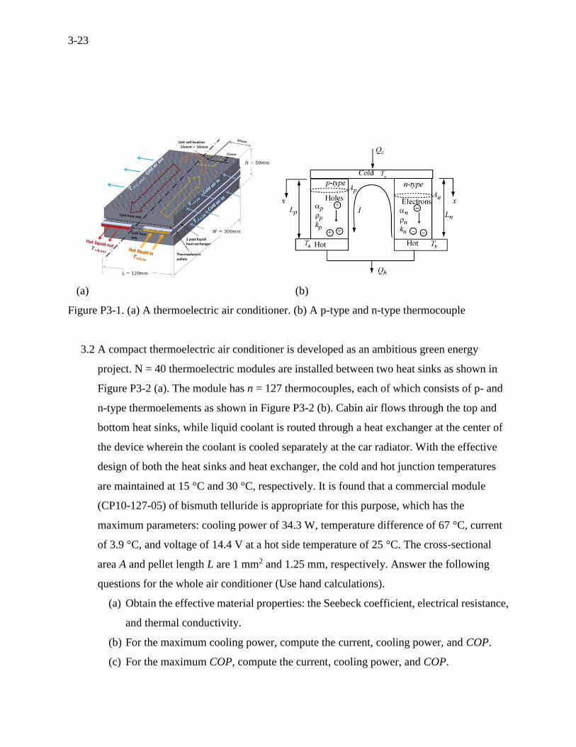
(a) (b)
Figure P3-1. (a) A thermoelectric air conditioner. (b) A p-type and n-type thermocouple
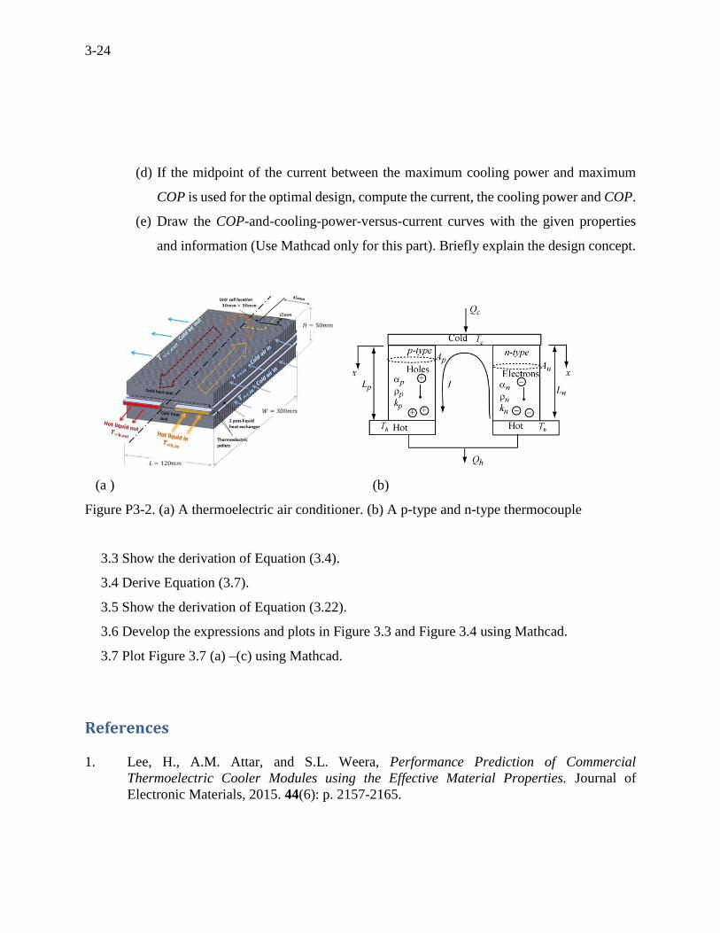
3.2 A compact thermoelectric air conditioner is developed as an ambitious green energy
project. N = 40 thermoelectric modules are installed between two heat sinks as shown in
Figure P3-2 (a). The module has n = 127 thermocouples, each of which consists of p- and
n-type thermoelements as shown in Figure P3-2 (b). Cabin air flows through the top and
bottom heat sinks, while liquid coolant is routed through a heat exchanger at the center of
the device wherein the coolant is cooled separately at the car radiator. With the effective
design of both the heat sinks and heat exchanger, the cold and hot junction temperatures
are maintained at 15 °C and 30 °C, respectively. It is found that a commercial module
(CP10-127-05) of bismuth telluride is appropriate for this purpose, which has the
maximum parameters: cooling power of 34.3 W, temperature difference of 67 °C, current
of 3.9 °C, and voltage of 14.4 V at a hot side temperature of 25 °C. The cross-sectional
area A and pellet length L are 1 mm2 and 1.25 mm, respectively. Answer the following
questions for the whole air conditioner (Use hand calculations).
(a) Obtain the effective material properties: the Seebeck coefficient, electrical resistance,
and thermal conductivity.
(b) For the maximum cooling power, compute the current, cooling power, and COP.
(c) For the maximum COP, compute the current, cooling power, and COP.
3-24
(d) If the midpoint of the current between the maximum cooling power and maximum
COP is used for the optimal design, compute the current, the cooling power and COP.
(e) Draw the COP-and-cooling-power-versus-current curves with the given properties
and information (Use Mathcad only for this part). Briefly explain the design concept.
(a ) (b)
Figure P3-2. (a) A thermoelectric air conditioner. (b) A p-type and n-type thermocouple
3.3 Show the derivation of Equation (3.4).
3.4 Derive Equation (3.7).
3.5 Show the derivation of Equation (3.22).
3.6 Develop the expressions and plots in Figure 3.3 and Figure 3.4 using Mathcad.
3.7 Plot Figure 3.7 (a) –(c) using Mathcad.
References
1. Lee, H., A.M. Attar, and S.L. Weera, Performance Prediction of Commercial
Thermoelectric Cooler Modules using the Effective Material Properties. Journal of
Electronic Materials, 2015. 44(6): p. 2157-2165.