Embed Size (px)
Citation preview

54
CHAPTER 2
MATERIALS AND METHODS
2.1 INTRODUCTION
This section of the research work describes the method of
production of ductile iron and carbidic ductile iron, its heat treatment process
and standards of different characterization. The experimental work and
characterization is done in two phases. An austempered ductile iron is
produced and analyzed in the first phase of the work.
The production of austempered ductile iron is done in two steps.
One is the production of ductile iron castings and the second is the
austempering heat treatment of the specimens. Then the austempered
specimens are subjected to various mechanical tests like tensile, hardness,
impact and abrasion wear test. Microstructure analysis is carried out and SEM
analysis is also carried out on the impact and the wear test specimens.
In the second phase of the research, the carbidic ductile iron is
produced by melting route. Different levels of chromium alloyed carbidic
ductile iron are produced with high chromium ferro-chrome as alloy addition.
Tensile, impact, hardness and wear test specimens are machined from the
casted Y-blocks. The carbidic ductile iron specimens are austempered to form
the carbidic austempered ductile iron. Mechanical properties of the CADI
specimens are measured, SEM analysis of impact fracture and wear surfaces
are also carried out.

55
2.2 PHASE I – PRODUCTION AND CHARACTERIZATION OF
DI AND ADI
2.2.1 Introduction
In the first phase of the experimental work ductile iron is casted and
austempered to get the austempered ductile iron. The base composition of
ductile cast iron is hypereutectic, where the carbon and silicon contents are
typically 3.7 and 2.5 respectively with a carbon equivalent (CE) of 4.5. High
silicon content is to be retained to get the spherical graphite because silicon is
a graphite stabilizer. The graphite nodules increase the mechanical properties
of the materials. Steel scraps, foundry returns and pig iron are melted in a
medium frequency induction furnace; composition is adjusted by adding shell
coke as the carburizer, Fe-Si for silicon increase and superheated to 1590oC.
Thus the first constituents appear during solidification are graphite nodules,
which nucleate and grow, without any martensite, but eventually with
austenite enclosing the graphite nodule.
The processing scheme utilized in the production of ductile iron
using a magnesium ferro-silicon alloy of 6-8% Mg (Fe-Si-Mg) includes the
following steps. The step by step process of the ductile iron production
process is explained in Figure 2.1.
1. Build a charge from steel scrap, foundry returns (risers, gates,
etc.) and pig iron.
2. Melt the charge and superheat to 1590oC.
3. Verify the composition and adjust the carbon and silicon levels.
4. Pour into magnesium treatment ladle covered with Fe-Si-Mgalloy.
5. Transfer into pouring ladle and inoculate with ferrosilicon
based inoculants.
6. Pour the melt into the prepared CO2 mould.

56
Figure 2.1 Flow chart of ductile iron production
2.2.2 Raw Material Selection
The raw materials are important for the production of ductile iron.
Final composition of the melt mainly depends on the raw materials used and
the final properties of the material. The charge consists of low manganese
steel scrap, foundry returns like runners, gates, shell coke, and pig iron.
2.2.3 Melting and Composition Control
An electric induction furnace is used for melting the base metal.
The basic melting processes are furnace operations including charging,
melting, composition analysis, composition adjustment, slag removal and
superheating. The raw materials are added to the melting furnace directly and
heated. The molten metal is tapped by tilting and pouring through the spout
for the magnesium treatment.
Raw Material Selection
Charging and Melting
Inoculation
Composition Control
Magnesium Treatment
Mould Making
Casting knockout
Pouring
Y-Block Casting
Alloy additions

57
2.2.4 Magnesium Treatment
It is the critical step in the ductile iron making. The amount of
residual magnesium present in the melt during solidification is in the range of
0.03 to 0.05 weight percent. Magnesium contents less than this amount will
result in flake graphite, and the amount more than this results in the
appearance of exploded graphite. Either of the type contributes to degradation
of the ductility of the cast iron.
The tundish cover ladle method is suitable for better magnesium
recovery. Figure 2.2 shows the design of a tundish cover ladle suitable for the
magnesium treatment. The use of a refractory dividing wall to form an alloy
pocket in the bottom of the ladle gives an improved Mg recovery. The
diameter of the filling hole is chosen to minimize the generation of fume
while allowing the ladle to be filled quickly without excessive temperature
loss. It is essential that the Fe-Si-Mg alloy is not exposed to the liquid iron
until quite late in the filling procedure, so the filling hole is positioned to
introduce liquid iron away from the alloy pocket in the ladle bottom.
Figure 2.2 Magnesium treatment process

58
The calculated amount of magnesium alloy is kept in the alloy
pocket and covered with steel turnings, Fe-Si pieces of size 25 × 6 mm. When
the melt level in the ladle reaches the dividing wall, iron flows over and forms
a semi-solid mass with the covered material allowing the ladle to be almost
filled before the reaction starts, thus ensuring good recovery of Mg. This is
done primarily to reduce the violence of the reaction that occurs when the
molten iron contacts the magnesium.
In order to minimize temperature losses during treatment, the ladle
and cover should be separately heated with gas burners before assembly. The
common magnesium treatment (Fe-Si-Mg) master alloy which is used in this
process contains approximately 6-wt% Mg, about 45 wt% Si, with the balance
Fe. About twice as much as magnesium is to be added during treatment and is
required in the casting (this represents a 50% recovery) because of the
oxidation losses during the violent treatment reaction.
Amount of melt = 50 kg
Magnesium content of the master alloy = 6 wt%
Expected recovery = 50%
Magnesium master alloy required = 1.5 kg/100 kg of metal.
During this time the magnesium reaction involves production of
bubbles of magnesium vapour which proceeds to rise up through the molten
iron bath which is now covering the pockets in the chamber. For successful
treatment results, there should be a significant portion of the magnesium is
dissolved into the molten iron, so that the correct conditions for graphite
nodule formation are met in the solidifying melt. Typical “recoveries” of
magnesium for the Tundish cover treatment facility are in the range of 50 - 60
percent. Successful nodularization requires a composition of about 0.03 to
0.05 weight percent elemental magnesium in the iron. It is necessary that
sulphur content should be kept below 0.015% for successful treatment,

59
because ability of the sulphur to react with the magnesium (forming Mg2S)
removes elemental magnesium from the melt. Often the melt needs to be
desulphurized before the treatment begins. It usually involves additions of Ca
(calcium) to combine with the sulphur. The calcium sulphide will rise to the
slag layer and be skimmed.
Tapping time is usually around 40 seconds. The temperature loss
during magnesium treatment is around 50°C, so the tapping temperature must
be adjusted accordingly; treatment temperatures around 1540°C are
commonly used. After treatment, the tundish cover is removed; the metal is
transferred to a pouring ladle where inoculation takes place. The liquid metal
must be poured within a short period of time after treatment, usually less than
5 minutes. Longer time may fade the magnesium in the liquid metal and lead
to the formation of vermicular cast iron with poor mechanical properties.
2.2.5 Inoculation
Immediately after magnesium treatment, the iron must be
inoculated. Graphitizing inoculant BACAL 25 is used. The inoculant
manufactured and supplied by M/s SNAM alloy is used. The BACAL
contains 25% barium and remaining calcium. Normally 0.3 wt percentage of
inoculants is added into the melt. Inoculation treatment is not permanent. The
inoculants effect starts to fade from the time it is added. Significant fading
occurs within five minutes of inoculation. As the inoculating effect fades, the
number of nodules formed decreases and the tendency to produce chill and
mottled iron increases. In addition, the quality of the graphite nodules
deteriorates and quasi-flake nodules occur.
2.2.6 Moulding, Pouring and Knockout
CO2 mould with designed runners and risers is prepared for the
Standard Y-block pattern as per the ASTM A 370 standards and the

60
dimensions are shown in Figure 2.3. Casting trials are done by filling the
molten metal through the designed runners and risers and checked for its
filling performance. This trial shows good filling performance of the mould.
The same design of runner and riser is used for the Y-block casting
production. The molten metal after treatment is poured into the mould within
a short span of time to avoid the fading of magnesium. The mould is allowed
to cool for a period of 12 hours and the casting is knocked off from the
mould. The casting is shot blasted to remove the sand particles on it. The
runner and the risers are removed from the casting using arc cutting. After
cleaning, the visual inspection is carried out on the Y- block that reveals
defect free cast surface. Cracks, blow holes, porosities are not observed on the
surfaces.
Figure 2.3 Standard dimensions of Y-block casting
2.2.7 Composition Analysis
The final composition of the specimen is analyzed using a vacuum
spectrometer. The results of the composition are shown in Table 2.1.
Specimens are machined from the lower part of the Y-block (Hatched lines
shown in Figure 2.3) for the characterization. Melt 1 is the common unalloyed
ductile iron (500/7) casting taken for the experimentation. Nodule count 80

61
should be the minimum requirement for effective austempering. Standard
wire cutting, machining and grinding operations are employed for specimen
preparation.
Table 2.1 Composition of melt 1 by wt%
MeltIdentification
C Si Mn P S Mg Cr Cu Mo
Melt 1 3.6840 2.5332 0.4841 0.029 0.010 0.0408 0.0267 0.0341 0.00
The microstructure of the melt 1 specimen is analyzed after
austempering. The microstructure does not reveal any formation of ausferrite
matrix. It contains graphite nodules in the pearlite and ferrite matrix.
Literatures show that small quantities of alloying are necessary for best
austempering. Hardenability elements are to be alloyed for the formation of
ausferrite matrix. Copper, nickel, chromium, titanium and molybdenum are
some of the hardenability agents used in ductile iron. In this study, copper and
molybdenum are added to get the austempered ductile iron.
Table 2.2 Composition of alloyed DI
Composition Melt 2 Melt 3C 3.5862% 3.3652%Si 2.4957% 2.8112%
Mn 0.4681% 0.2657%P 0.0240% 0.0410%S 0.008% 0.0070%
Mg 0.0490% 0.0320%Cr 0.0256% 0.0410%Cu 0.3145% 0.3600%Mo 0.0000% 0.4200%

62
Selection of the raw material and the melting is carried out as in the
previous case. Calculated amount of copper for melt 2, copper and
molybdenum for melt 3 are added in the raw materials. Recovery of 60% of
the alloying elements is considered. Weight of the melt is 50 kg. Addition of
copper turnings for the melt 2 is 300 grams. 300 grams of copper turnings and
700 grams of HCFeMo are added to the melt 3 to increase the content of
copper and molybdenum. The composition of the Y-block castings is checked
using spectrometer and the same has been given in Table 2.2.
Microstructures of the melt 2 and 3 are analyzed after austempering
treatment. The microstructure reveals ausferrite matrix. The fact sheet of
complete experimentation and characterization of austempered ductile iron is
shown in Figure 2.4.
2.2.8 Specimen Preparation
Specimens are machined from the lower part of the Y-block for the
tensile test, hardness test, wear test and impact toughness test. The positions
of the specimens in the Y-block are marked as hatching lines in Figure 2.3.
10mm x10mm size bars are cut from the Y-block casting by hacksaw cutting.
These bars are milled to the Charpy impact test specimen of dimensions
10mmx10mmx55mm as per ASTM A370 standard. The standard tensile test
specimen, hardness test specimen and the wear test specimens are turned in
lathe.
2.2.9 Austempering Heat Treatment Process
Austempered ductile iron is produced by heat-treating the cast
ductile iron alloyed with small amounts of copper and molybdenum. The final
properties of the material are determined by careful choice of heat treatment
parameters. The austempering process improves the strength of the specimens
with minimal distortion and stresses. Austempering heat treatment process is
a two stage process. During the first stage the specimens are heated to
63
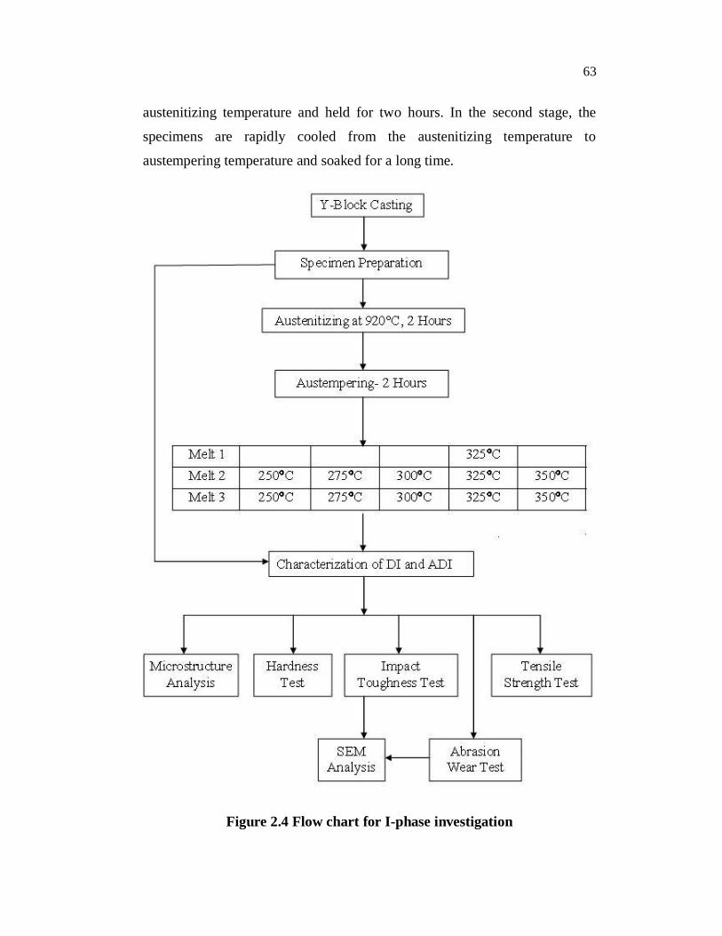
austenitizing temperature and held for two hours. In the second stage, the
specimens are rapidly cooled from the austenitizing temperature to
austempering temperature and soaked for a long time.
Figure 2.4 Flow chart for I-phase investigation

64
The steps followed in the austempering process are:
1. Heating to the austenitizing temperature (A to B) – 920°C.
2. Austenitizing (B to C) at 920°C for two hours.
3. Rapid cooling to the austempering temperatures (C to D) like
250°C, 275°C, 300°C, 325°C and 350°C.
4. Isothermal heat treatment at the austempering temperature for
two hours (D to E).
5. Air cooling to room temperature (E to F).
Figure 2.5 shows a schematic of the austempering process.
Figure 2.5 Schematic of the austempering process
Two electrical resistance type salt bath furnaces (Figure 2.6) are
used for the austempering process. One is for austenitizing and another is for
austempering. Furnace system and process are driven via a state-of-art human
machine interface, which also provides access to the heat treatment
programmes. Flexibility in the furnace and controller configurations allows
the austempering process to be tailored to the part.

65
The specimens are immersed in the crucible containing the molten
salt bath. The mode of heat transfer to the work piece is by convection
through the liquid bath. These salt bath offers certain advantages over other
quench medium.
All work pieces are at uniform temperature and have identical
surroundings. Such a condition results in better surface
conditions and consistent and reproducible results.
Since work piece is in direct contact with the molten bath, there
is no danger of oxidation and/or decarburization.
Salt bath also reduces the fluctuations of temperature.
The commonly used salts are nitrates, carbonates, chlorides,
cyanides and caustic soda. The composition of salt bath used for the
austenization and the austempering process are tabulated in Table 2.3. The
salt is managed and reused to obviate environmental damage.
Table 2.3 Salt bath composition and working temperature
Working Temperature Composition of Salt BathAustenitizationWorking temperature range:650 C -1050 C
Sodium Nitrate = 50%Potassium Nitrate = 50%
AustemperingWorking temperature range:175 – 540 C
Sodium Nitrate =13%Potassium Nitrate = 50%Sodium nitrite = 37%

66
Figure 2.6 Electric resistance furnace (A) Austenitizing (B) Austempering
The choice of austenitizing temperature depends on the chemical
composition of the ductile iron. The time of austenitizing is as important as
the choice of temperature. The austenitizing temperature should be so chosen
that the component is in the austenite + graphite ( + G) phase.
Elements like silicon raise the upper critical temperature (UCT)
while manganese will lower it. If the austenitizing temperature is below the
UCT or in the subcritical range ( + + G), then proeutectoid ferrite will be
present in the final microstructure, resulting in a lower strength and hardness
of the material. Once the proeutectoid ferrite is formed, the only way to
eliminate is reheat it above the UCT. The ductile iron components should be
held for a sufficient time to create an austenite matrix saturated with carbon.
This time is additionally affected by the alloy content of the ductile iron. Iron
with heavily alloyed material takes longer time to austenitizing. In this study,
the samples are austenitised at 920°C for a time of 2 hours and then
austempered.
Cooling from the austenitizing temperature to the austempering
temperature (Figure 2.5 C to D) must be completed rapidly enough to avoid

67
the formation of pearlite. The austenitized specimens are transferred to
austempering salt bath within five seconds. If pearlite is formed, the strength,
elongation and toughness will be reduced.
The formation of pearlite can be caused by several things, most
notably a lack of quench severity or a low hardenability for the effective
section size. The traditional quench media, oil and water are not used so that
the load does not reach the Ms temperature and brittle martensite cannot
develop. It is possible to increase the quench severity of molten salt quench
baths by making water additions. By inoculating the salt bath with water,
quenching rates are enhanced to allow treatment of larger section parts
without adjustment of cast composition. The range of the austempering
temperature for the production of ADI and CADI is 250 to 400°C.
Austempering time also varied between one and four hours in a time interval
of one hour for CADI production. The austempering temperature and time
decides the final properties of the austempered ductile iron and carbidic
austempered ductile iron. Higher grades of ADI are produced at lower quench
temperatures.
Once the austempering process is completed and the ausferrite has
been produced, the components are cooled to room temperature. The cooling
rate will not affect the final microstructure and final properties of ADI as the
carbon content of the austenite is high enough to lower the martensite start
temperature to a temperature significantly below room temperature.
2.2.10 Characterization
2.2.10.1 Metallographic examination
It remains the most important tool for the study of micro-
constitutions in the material. The metallographic sample preparation is carried

68
out by using standard techniques. The specimen for microscopic examination
is made flat using grinding wheel and then polished with various grades of
emery sheets, followed by disc polishing using diamond paste to reveal the
microstructure. The polished samples are etched with 5% nital. The etched
specimen microstructure is analyzed and then photograph is taken using the
Nikon Epiphot-Dx optical microscope (shown in Figure 2.7) equipped with
high resolution digital camera at various magnifications.
Figure 2.7 Metallurgical microscope
2.2.10.2 Hardness test
Brinell hardness is determined by forcing a hard steel ball of
specified diameter under a specified load on the surface of the specimen and
measuring the diameter of the indentation left after the test. The Brinell
hardness number is obtained by dividing the load used, in kilograms, by the
actual surface area of the indentation in square millimeters. The result is a
pressure measurement, but the units are rarely stated. The size of the
specimen used for the hardness test is shown in Figure 2.8.

69
Figure 2.8 Brinell hardness test specimen
The Brinell hardness tester is shown in Figure 2.9. The Brinell
hardness test is conducted as per the ASTM E10 standard and the methodconsists of indenting the test material with a 10 mm (D) diameter hardened
steel ball subjected to a load (P) of 3000 kgf. The full load is applied for 10 to15 seconds on the specimens. The diameter of the indentation (d) left in the
test material is measured using powered microscope with a least count of 0.01mm. The Brinell harness number is calculated by using Equation (2.1).
2 2
2PHBND(D (D d )
(2.1)
Figure 2.9 (A) Indentation (B) Brinell hardness testing machine
All Dimensions are in mm

70
The diameter of the impression is the average of two readings at
right angles of an impression and four impressions per specimen are carried
out. Compared to the other hardness test methods, the Brinell ball makes the
deepest and widest indentation, so the test averages the hardness over a wider
amount of material, which will more accurately account for multiple grain
structures and any irregularities in the uniformity of the material. This method
is the best one for achieving the bulk or macro-hardness of a material,
particularly those materials with heterogeneous structures.
2.2.10.3 Impact toughness test
Impact toughness is a measure of the energy absorbed during the
fracture of a specimen of standard dimensions and geometry when subjected
to impact loading. The Charpy impact test is a standardized high strain-rate
test, which determines the amount of energy absorbed by the material during
fracture. This absorbed energy is the measure of toughness of the given
material.
Figure 2.10 Charpy impact testing machine
Charpy impact toughness test is conducted as per ASTM E 23
standard at room temperature using a charpy impact testing machine with 300

71
joules hammer capacity and 4.5ms-1striking velocity. The pendulum type
charpy impact test equipment set up is shown in Figure 2.10. Tests are
conducted on unnotched test samples of size 10mm x 10mm x 55mm and the
average of the two impact values is considered. The standard charpy impact
test specimen is shown in Figure 2.11. It is widely applied in industry, as it is
easy to prepare and conduct and results can be obtained quickly and cheaply.
Figure 2.11 ASTM standard charpy test specimen
The qualitative results of the impact test can be used to determine
the ductility and strength of the material. Materials with high strength and
high ductility exhibits high toughness and the materials of low strength and
high ductility have low impact toughness. If the material breaks on a flat
plane, the fracture is brittle, and if the material breaks with jagged edges or
shear lips, then the fracture is ductile.
2.2.10.4 Ultimate tensile strength test
The ultimate tensile strength is the maximum stress that can besustained by a structure in gradually increasing tensile load that is applied
uniaxially along the long axis of the specimen. If the stress is applied andmaintained, fracture will be the result. Tensile specimens are machined as per
the standards of ASTM A 370 and heat treated. The standard dimensions ofthe tensile test specimen are shown in Figure 2.12. The tensile test is
conducted in a micro tensile testing machine of 2000 N capacity and theultimate tensile strength of the specimen is calculated. Two tensile samples in
All dimensions are in mm

72
each condition are prepared and tested. Average of these two readings isconsidered for discussion.
Figure 2.12 Tensile test specimen
2.2.10.5 Wear test
Pin-on-disk abrasive test is a commonly used technique for
investigating abrasive wear of the material. Pin-on-disk is an apparatus thatconsists essentially of a “pin” in contact with a rotating disk. The pin can bethe test piece of interest. The contact surface of the pin is flat. A pre-determined load is also applied to the specimen. The disk revolves in a
particular speed, and an appropriate track on the disk is selected based onthe velocity of the travel required. In a typical pin-on-disk experiment,the material removed is determined by weighing and/or measuring the weightof the specimen. The schematic of the abrasive wear test is shown in
Figure 2.13.
Figure 2.13 Schematic diagram of abrasive wear test

73
Figure 2.14 Pin-on-disk machine setup
Figure 2.14 shows the pin-on-disk machine setup. The main
variables that affect friction and wear are the velocity and the normal load. In
addition, specimen orientation can be important if retained wear debris affects
the wear rate. Most commercial pin-on-disk testers use high loads (e.g.100-
1000N) obtained with dead weight and large areas of contact.
Figure 2.15 Wear test specimen
Abrasion wear resistance of the material is measured as per ASTM
standard G99-05 using Pin-on-disk wear testing machine. The material to be
tested is made in the form of a pin with dimensions 10mm diameter and
All dimensions are in mm

74
20mm long cylinder as shown in Figure 2.15. The pin is weighed using the
balance. It is fixed in the specimen holder and kept pressed against the wear
disc in the machine using predetermined load. Disk hardness of HRC – 65,
Load of 98.1N is applied to the specimen, with a travel velocity of one m/s
and a distance of 10,000m is considered for the measurement of weight loss.
The specimen is removed and weighed. The weight loss is noted. The weights
are measured by means of 0.01 mg precision scale.
2.2.10.6 SEM analysis
The scanning electron microscope (SEM) is shown in Figure 2.16,
which provides a valuable combination of high resolution imaging. The big
advantage of SEM is that the sample surface can be examined directly with a
depth of field very much greater than that of the optical microscope at high
magnifications (>100,000x) and in some cases with better resolution.
Figure 2.16 Scanning electron microscope setup
The impact fractured surface is analyzed using Scanning Electron
Microscope of JEOL MODEL JSM 6360 with magnification minimum of 25x
and maximum of 2 lakhs. The result is a television-type image of the portion

75
of the sample surfaces being scanned by the beam. By studying the fracture
surface the mode of fracture is whether ductile or brittle has to be established.
Ductile Fracture: Ductile fracture has been defined rather
ambiguously as fracture occurring with appreciable gross plastic deformation.
Another important characteristic of ductile fracture is that it occurs by a slow
tearing of the metal with the expenditure of considerable energy. Ductile
fracture can take several forms of single crystals of HCP metals and may slip
on successive basal plans until the final crystal separates by shear. A shear
fracture occurs as a result of extensive slip on the active plan. A fractured
surface that is caused by shear appears at low magnifications to be grey and
fibrous. Dimpled rupture is characterized by cup like dispersions. This type of
fractured surface denotes a ductile facture.
Brittle Fracture: Cleavage fracture represents brittle fracture that
occurs along crystallographic planes. The characteristic feature of cleavage
fracture is flat face. The flat faces exhibit river marking. The river marking
are caused by crack moving through the crystal along a number of parallel
planes which forms a series of plateaus and connecting edges. The direction
of river pattern represents the direction of crack propagation.
2.3 PHASE II - PRODUCTION AND CHARACTERIZATION OF
CADI
2.3.1 Introduction
This phase of the experimental work describes the production and
the characterization of Carbidic Austempered Ductile iron. Carbidic ductile
iron is a ductile cast iron containing carbides in the pearlite and ferrite matrix
(they are either thermally or mechanically induced), and that is subsequently
austempered to produce an ausferrite matrix with an engineered amount of
carbides. The final material is called as carbidic austempered ductile iron.

76
Carbides in the ductile iron is induced by
Reducing the graphitizing elements such as silicon.
Increasing the cooling rate of solidification by using chills.
Introducing carbide stabilizing elements like chromium,
manganese, molybdenum and titanium.
The melt with suitable carbide stabilizing elements is treated with
magnesium and/or rare earths result in spheroidal graphite with carbides in
the microstructure. Carbides are stable and tend to retain their as-cast volume
fractions after austenitizing (Hayrynen et al 2003). The carbides produced
from this technique cannot be “dissolved” by subsequent austempering heat
treatment. The carbidic austempered ductile iron is formed by austempering
the produced chromium alloyed ductile iron and characterized. Impact
fractured surface and wear surfaces are analyzed using SEM.
2.3.2 Production of CADI
The charge for the production of carbidic ductile iron consists of
foundry returns like runners, gates, shell coke, ore with 3 to 4.5 % carbon,
50% pig iron ingot and low manganese steel scrap. An electric induction
furnace is used for the melting of base metal. The basic melting process are
furnace operations including charging, melting, composition analysis,
composition adjustment and superheating. The raw materials and fluxes are
added into the melting furnace directly. After melting the slag is removed
from melt.
Now the high-carbon ferro-chromium is added into the melt to
increase the chromium level. The expected amount of chromium in the high
carbon ferrochromium alloy is around 60 %. The amount of chromium alloy

77
added for each 50 kg melt is given in Table 2.4. After the addition of
chromium the molten metal is tapped for magnesium treatment. Now the
melt is magnesium treated by following the standard procedure and then
inoculated. The amount of inoculants added to this melt is reduced by 10%
compared to the regular ductile iron. The inoculants are used as much the
formation of alloy carbide is not effective.
Table 2.4 Amount of chromium alloy added to the melt for CADI
MeltIdentification
Planned ChromiumContent
Alloyused
Amount ofchromium alloy
added (kg)1% Cr 1 wt% HCFeCr 0.83
0.8% Cr 0.8 wt% HCFeCr 0.670.6% Cr 0.6 wt% HCFeCr 0.500.4% Cr 0.4 wt% HCFeCr 0.33
Standard Y-block carbon di-oxide mould is made by machine
moulding. Magnesium treated and inoculated melt is poured into the mould.
After solidification and curing, Y-block is knocked out from the mould,
runners and risers are removed from the casting and afterwards shot blasted.
The material in the as-cast condition is called as carbidic ductile iron. Y-
blocks are macro examined for porosity and blow holes by the naked eye.
Castings without porosity are used for further specimen preparation and
austempering heat treatment. Some of the specimens are tested in the as-cast
condition.
The composition of the Y-blocks after casting is measured using a
vacuum spectrometer. The amount of the other elements is kept constant
except the content of chromium. The amount of chromium is varied from
0.4% to 1.0%. Specimens for metallographic examination, hardness test,

78
impact toughness test, tensile test and wear test from all the compositions of
defect free Y-blocks are machined. Austempering heat treatment is carried out
by following the procedures explained under section 2.2.9. The specimens are
austenitized at 920°C for two hours and austempered at different temperatures
of 250°C, 300°C, 350°C and 400°C. The time of austempering is varied from
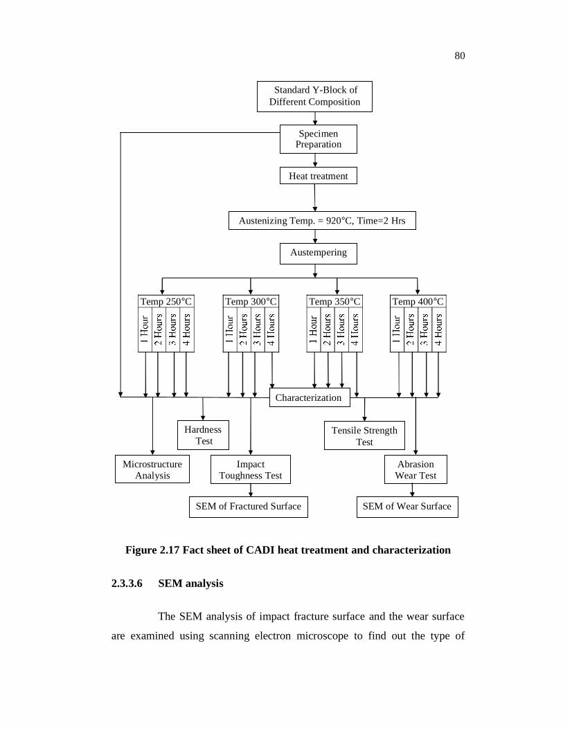
one hour to four hours with an interval of one hour. The heat treatment
process and characterization of the carbidic austempered ductile iron is shown
as fact sheet in Figure 2.17.
2.3.3 Characterization of CADI
Mechanical properties of the carbidic austempered ductile iron like
tensile strength, hardness, impact toughness and wear loss are measured. The
methods of measurement of these mechanical properties are done by
following the standard procedures.
2.3.3.1 Metallographic examination
The metallographic examinations on the carbidic ductile iron and
the carbidic austempered ductile iron are carried out using optical microscope.
The standard specimen preparation procedures are explained in section
2.2.10.1. The specimens are polished, etched in 10 % ammonium persulphate
and the volume percentage of carbide is measured using Neophot microscope
and “Metal Plus Version-1.0” image analysis software. The ASTM
designation E562-89 describes systematically manual point counting
procedure for statistically estimating the volume fraction of an identified
phase from sections through the microstructure. Ammonium persulphate
etchant is used to find the amount of carbides. This ammonium persulphate
tints the matrix dark and leaves the carbides as white. The micro-photographs
of CADI are taken by using 5% nital etching.
79
2.3.3.2 Hardness test
Brinell hardness test is conducted on the as-cast carbidic ductile
iron and the carbidic austempered ductile iron. The standard dimensions of
the specimen and the experiment producers have been explained in section
2.2.10.2.
2.3.3.3 Impact toughness test
Charpy impact toughness test is conducted on the as-cast carbidic
ductile iron and the carbidic austempered ductile iron. The standard
dimensions of the specimen and the experiment producers have been
explained in section 2.2.10.3.
2.3.3.4 Ultimate tensile strength test
Ultimate tensile strength test is conducted on the as-cast carbidic
ductile iron and the carbidic austempered ductile iron. The standard
dimensions of the specimen and the experiment producers have been
explained in section 2.2.10.4.
2.3.3.5 Wear test
Pin-on-disk wear abrasion test is conducted on the as-cast carbidic
ductile iron and the carbidic austempered ductile iron. The standard
dimensions of the specimen and the experiment producers have been
explained in section 2.2.10.5.
80
SpecimenPreparation
Heat treatment
Austenizing Temp. = 920°C, Time=2 Hrs
Austempering
Characterization
Tensile StrengthTest
Hardness Test
AbrasionWear Test
ImpactToughness Test
SEM of Fractured Surface SEM of Wear Surface
MicrostructureAnalysis
Temp 250°C Temp 300°C Temp 350°C Temp 400°C
Standard Y-Block ofDifferent Composition
Figure 2.17 Fact sheet of CADI heat treatment and characterization
2.3.3.6 SEM analysis
The SEM analysis of impact fracture surface and the wear surface
are examined using scanning electron microscope to find out the type of

81
fracture mechanism. The procedure to carry out this examination is explained
in section 2.2.10.6.
2.4 TAGUCHI METHOD
Taguchi method provides a systematic and efficient approach for
conducting experimentation to determine the optimum settings of design
parameters for performance and cost. The Taguchi method utilizes orthogonal
array to study a large number of variables with a small number of
experiments. It can reduce development cost by simultaneously studying a
large number of parameters. Using orthogonal arrays, the method can
significantly reduce the number of experimental configurations. The
conclusions drawn from small scale experiments are valid over the entire
experimental region spanned by the control factors and their settings.
2.4.1 Design of Experiments
Two major steps are involved in the production of carbidic
austempered ductile iron, one is casting and the other one is austempering
heat treatment. Composition of the material is the most important factor when
compared to the other factors like hardness of the mould, the filling velocity
of the melt, gating design etc. So the composition, particularly the chromium
content affects the properties of CADI.
In the heat treatment process, austenitizing temperature and time, as
well as austempering temperature and time are the controllable parameters.
Austempering temperatures and time are taken into account for the present
study. Therefore, three major factors have influence over the production of
the CADI. They are chromium content, austempering temperature and
austempering time. Four levels in each process parameter are selected and the
level values are shown in Table 2.5.

82
Table 2.5 Factors and levels – L16 (43)
LevelsCode Factors
1 2 3 4% Cr Chromium Percentage 0.4 0.6 0.8 1.0
TAAustempering
Temperature (ºC) 250 300 350 400
tAAustempering Time
(Hours) 1 2 3 4
The Taguchi method provides the laying out of the experimental
conditions using specially designed tables called Orthogonal Array (OA).
Taguchi orthogonal array is used for the selection of experiments at different
levels among the entire parameter space. An appropriate orthogonal array of
L16 (43) is selected using the Minitab -15 software based on the number of
factors and its levels. This orthogonal array shown in Table 2.6 gives the
number of experiments to be conducted with their factor levels.
This array consists of 16 rows, each representing an experiment
with factor level; the columns are assigned to the factors. The plan of
experiments is made of 16 tests in which the first column is assigned to the
chromium content (% Cr), second column for the austempering temperature
(TA) and the third column for the austempering time (tA).
After completion of all the experiments, the data are considered as
per the orthogonal array and S/N ratio of individual performance is computed.
A grey relational co-efficient and grey relational grade for all S/N ratios is
calculated. The major influencing parameters on the mechanical properties
are assessed by using ANOVA and optimal parameters are predicted for the
CADI production.

83
Table 2.6 L16 Orthogonal array
Levels of input parametersTrialNo % Cr TA tA
1 1 1 12 1 2 23 1 3 34 1 4 45 2 1 26 2 2 17 2 3 48 2 4 39 3 1 310 3 2 411 3 3 112 3 4 213 4 1 414 4 2 315 4 3 216 4 4 1
2.5 FIELD TEST
Ploughing conditions often cause excessive wear of agriculture
ploughshares. The hard particles like SiO2 and quartz present in the soil cause
high degree of wear on the ploughshares. The hardness of these particles are
beyond 900 HV. The ploughshares are also subjected to very highly
complicated dynamic stresses during ploughing. So far, forged steel (EN 45
steel) has been the material used as ploughshare in Tamilnadu. Often this
forged steel withstands the dynamic stresses developed during ploughing
rather than the wear. The wear resistance of the forged steel is very less.

84
Figure 2.18 Plough point
One of the major expected applications of ADI and the CADI is
agricultural equipments. As infield test, the developed CADI material is used
as plough point and its wear behavior is checked. The used plough point is
shown in Figure 2.18. The plough points are attached to the ploughshare of a
tractor using threaded fasteners. Three types of plough points are prepared.
One is 1% chromium as cast carbidic ductile iron and the other is the 1%
chromium CADI heat treated at 920°C, two hours as austenitizing and 300°C,
2 hour time as austempering conditions. The third is the regularly used forged
steel plough point as reference. The test is conducted at Mettupalayam area
of Coimbatore district. The as-cast material and CADI worked well as plough
point. The material loss is calculated after 40 hours of ploughing.