Embed Size (px)
Citation preview
Chapter 16. Particle Swarm Optimization
Chapter 16: Particle Swarm Optimization
Computational Intelligence: Second Edition
Computational Intelligence: Second Edition Chapter 16: Particle Swarm Optimization
Chapter 16. Particle Swarm Optimization
IntroductionOverview of the basic PSOGlobal Best PSOLocal Best PSOAspects of Basic PSOBasic Variations of PSOPSO ParametersParticle TrajectoriesSingle-Solution Particle Swarm Optimizers
Contents
IntroductionOverview of the basic PSOGlobal Best PSOLocal Best PSOAspects of Basic PSOBasic Variations of PSOPSO ParametersParticle TrajectoriesSingle-Solution Particle Swarm Optimizers
References102
Computational Intelligence: Second Edition Chapter 16: Particle Swarm Optimization
Chapter 16. Particle Swarm Optimization
IntroductionOverview of the basic PSOGlobal Best PSOLocal Best PSOAspects of Basic PSOBasic Variations of PSOPSO ParametersParticle TrajectoriesSingle-Solution Particle Swarm Optimizers
Introduction
Particle swarm optimization (PSO):developed by Kennedy & Eberhart [3, 7],first published in 1995, andwith an exponential increase in the number of publicationssince then.
What is PSO?a simple, computationally efficient optimization methodpopulation-based, stochastic searchbased on a social-psychological model of social influence andsocial learning [8]individuals follow a very simple behavior: emulate the successof neighboring individualsemergent behavior: discovery of optimal regions in highdimensional search spaces
Computational Intelligence: Second Edition Chapter 16: Particle Swarm Optimization

Chapter 16. Particle Swarm Optimization
IntroductionOverview of the basic PSOGlobal Best PSOLocal Best PSOAspects of Basic PSOBasic Variations of PSOPSO ParametersParticle TrajectoriesSingle-Solution Particle Swarm Optimizers
Introduction: What are the origins of PSO?
In the work of Reynolds on “boids” [12]: Flocking is anemergent behavior which arises from the interaction of simplerules:
Collision avoidanceVelocity matchingFlock centering
The work of Heppner and Grenander on using a “rooster” asan attractor [5]
Simplified social model of determining nearest neighbors andvelocity matching
Computational Intelligence: Second Edition Chapter 16: Particle Swarm Optimization
Chapter 16. Particle Swarm Optimization
IntroductionOverview of the basic PSOGlobal Best PSOLocal Best PSOAspects of Basic PSOBasic Variations of PSOPSO ParametersParticle TrajectoriesSingle-Solution Particle Swarm Optimizers
Origins of PSO (cont)
Initial objective: to simulate the graceful, unpredictablechoreography of collision-proof birds in a flock
At each iteration, each individual determines its nearestneighbor and replaces its velocity with that of its neighbor
Resulted in synchronous movement of the flock
Random adjustments to velocities prevented individuals tosettle too quickly on an unchanging direction
Adding roosters as attractors:
personal bestneighborhood best→ particle swarm optimization
Computational Intelligence: Second Edition Chapter 16: Particle Swarm Optimization
Chapter 16. Particle Swarm Optimization
IntroductionOverview of the basic PSOGlobal Best PSOLocal Best PSOAspects of Basic PSOBasic Variations of PSOPSO ParametersParticle TrajectoriesSingle-Solution Particle Swarm Optimizers
Overview of basic PSO
What are the main components?A swarm of particlesEach particle represents a candidate solutionElements of a particle represent parameters to be optimized
The search process:Position updates
xi (t + 1) = xi (t) + vi (t + 1)
wherexij(0) ∼ U(xmin,j , xmax,j)
Velocitydrives the optimization processstep sizereflects experiential knowledge and socially exchangedinformation
Computational Intelligence: Second Edition Chapter 16: Particle Swarm Optimization
Chapter 16. Particle Swarm Optimization
IntroductionOverview of the basic PSOGlobal Best PSOLocal Best PSOAspects of Basic PSOBasic Variations of PSOPSO ParametersParticle TrajectoriesSingle-Solution Particle Swarm Optimizers
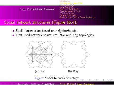
Social network structures (Figure 16.4):
Social interaction based on neighborhoodsFirst used network structures: star and ring topologies
(a) Star (b) Ring
Figure: Social Network Structures
Computational Intelligence: Second Edition Chapter 16: Particle Swarm Optimization

Chapter 16. Particle Swarm Optimization
IntroductionOverview of the basic PSOGlobal Best PSOLocal Best PSOAspects of Basic PSOBasic Variations of PSOPSO ParametersParticle TrajectoriesSingle-Solution Particle Swarm Optimizers
Other social structures (Figure 16.4):
(a) Von Neumann (b) Pyramid
Figure: Advanced Social Network Structures
Computational Intelligence: Second Edition Chapter 16: Particle Swarm Optimization

Chapter 16. Particle Swarm Optimization
IntroductionOverview of the basic PSOGlobal Best PSOLocal Best PSOAspects of Basic PSOBasic Variations of PSOPSO ParametersParticle TrajectoriesSingle-Solution Particle Swarm Optimizers
Other social structures (cont...)
(a) Clusters (b) Wheel
Figure: Advanced Social Network Structures
Computational Intelligence: Second Edition Chapter 16: Particle Swarm Optimization
Chapter 16. Particle Swarm Optimization
IntroductionOverview of the basic PSOGlobal Best PSOLocal Best PSOAspects of Basic PSOBasic Variations of PSOPSO ParametersParticle TrajectoriesSingle-Solution Particle Swarm Optimizers
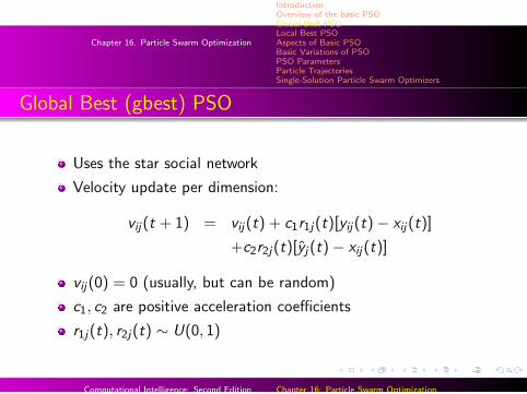
Global Best (gbest) PSO
Uses the star social network
Velocity update per dimension:
vij(t + 1) = vij(t) + c1r1j(t)[yij(t)− xij(t)]
+c2r2j(t)[yj(t)− xij(t)]
vij(0) = 0 (usually, but can be random)
c1, c2 are positive acceleration coefficients
r1j(t), r2j(t) ∼ U(0, 1)
Computational Intelligence: Second Edition Chapter 16: Particle Swarm Optimization
Chapter 16. Particle Swarm Optimization
IntroductionOverview of the basic PSOGlobal Best PSOLocal Best PSOAspects of Basic PSOBasic Variations of PSOPSO ParametersParticle TrajectoriesSingle-Solution Particle Swarm Optimizers
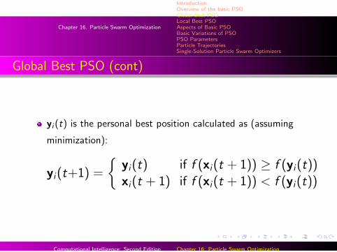
Global Best PSO (cont)
yi (t) is the personal best position calculated as (assuming
minimization):
yi(t+1) =
{yi(t) if f (xi(t + 1)) ≥ f (yi(t))xi(t + 1) if f (xi(t + 1)) < f (yi(t))
Computational Intelligence: Second Edition Chapter 16: Particle Swarm Optimization
Chapter 16. Particle Swarm Optimization
IntroductionOverview of the basic PSOGlobal Best PSOLocal Best PSOAspects of Basic PSOBasic Variations of PSOPSO ParametersParticle TrajectoriesSingle-Solution Particle Swarm Optimizers
Global Best PSO (cont)
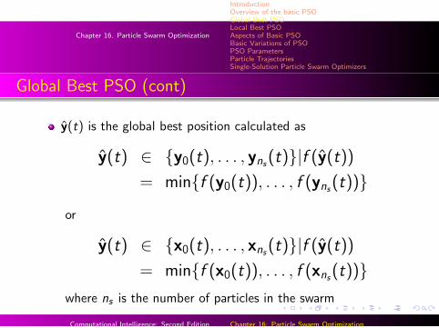
y(t) is the global best position calculated as
y(t) ∈ {y0(t), . . . , yns(t)}|f (y(t))
= min{f (y0(t)), . . . , f (yns(t))}
or
y(t) ∈ {x0(t), . . . , xns(t)}|f (y(t))
= min{f (x0(t)), . . . , f (xns(t))}
where ns is the number of particles in the swarm
Computational Intelligence: Second Edition Chapter 16: Particle Swarm Optimization
Chapter 16. Particle Swarm Optimization
IntroductionOverview of the basic PSOGlobal Best PSOLocal Best PSOAspects of Basic PSOBasic Variations of PSOPSO ParametersParticle TrajectoriesSingle-Solution Particle Swarm Optimizers
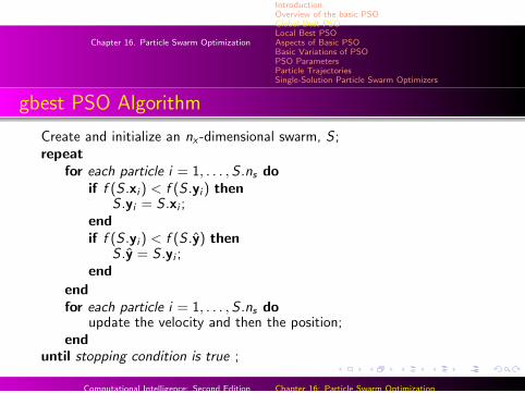
gbest PSO Algorithm
Create and initialize an nx -dimensional swarm, S ;repeat
for each particle i = 1, . . . ,S .ns doif f (S .xi ) < f (S .yi ) then
S .yi = S .xi ;endif f (S .yi ) < f (S .y) then
S .y = S .yi ;end
endfor each particle i = 1, . . . ,S .ns do
update the velocity and then the position;end
until stopping condition is true ;
Computational Intelligence: Second Edition Chapter 16: Particle Swarm Optimization
Chapter 16. Particle Swarm Optimization
IntroductionOverview of the basic PSOGlobal Best PSOLocal Best PSOAspects of Basic PSOBasic Variations of PSOPSO ParametersParticle TrajectoriesSingle-Solution Particle Swarm Optimizers
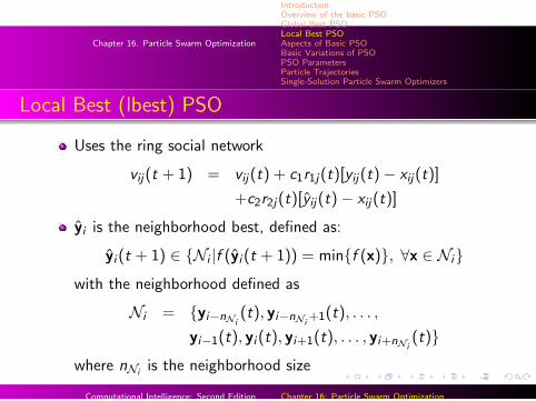
Local Best (lbest) PSO
Uses the ring social network
vij(t + 1) = vij(t) + c1r1j(t)[yij(t)− xij(t)]
+c2r2j(t)[yij(t)− xij(t)]
yi is the neighborhood best, defined as:
yi (t + 1) ∈ {Ni |f (yi (t + 1)) = min{f (x)}, ∀x ∈ Ni}
with the neighborhood defined as
Ni = {yi−nNi(t), yi−nNi
+1(t), . . . ,
yi−1(t), yi (t), yi+1(t), . . . , yi+nNi(t)}
where nNiis the neighborhood size
Computational Intelligence: Second Edition Chapter 16: Particle Swarm Optimization
Chapter 16. Particle Swarm Optimization
IntroductionOverview of the basic PSOGlobal Best PSOLocal Best PSOAspects of Basic PSOBasic Variations of PSOPSO ParametersParticle TrajectoriesSingle-Solution Particle Swarm Optimizers
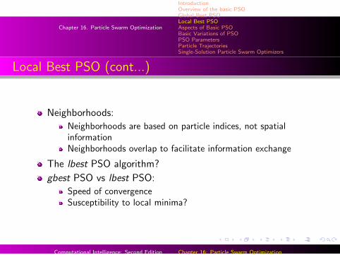
Local Best PSO (cont...)
Neighborhoods:
Neighborhoods are based on particle indices, not spatialinformationNeighborhoods overlap to facilitate information exchange
The lbest PSO algorithm?
gbest PSO vs lbest PSO:
Speed of convergenceSusceptibility to local minima?
Computational Intelligence: Second Edition Chapter 16: Particle Swarm Optimization

Chapter 16. Particle Swarm Optimization
IntroductionOverview of the basic PSOGlobal Best PSOLocal Best PSOAspects of Basic PSOBasic Variations of PSOPSO ParametersParticle TrajectoriesSingle-Solution Particle Swarm Optimizers
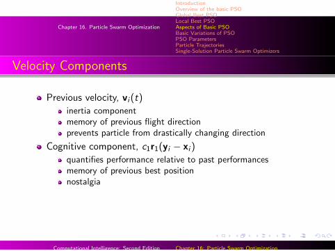
Velocity Components
Previous velocity, vi (t)
inertia componentmemory of previous flight directionprevents particle from drastically changing direction
Cognitive component, c1r1(yi − xi )
quantifies performance relative to past performancesmemory of previous best positionnostalgia
Social component, c2r2(yi − xi )
quantifies performance relative to neighborsenvy
Computational Intelligence: Second Edition Chapter 16: Particle Swarm Optimization
Chapter 16. Particle Swarm Optimization
IntroductionOverview of the basic PSOGlobal Best PSOLocal Best PSOAspects of Basic PSOBasic Variations of PSOPSO ParametersParticle TrajectoriesSingle-Solution Particle Swarm Optimizers
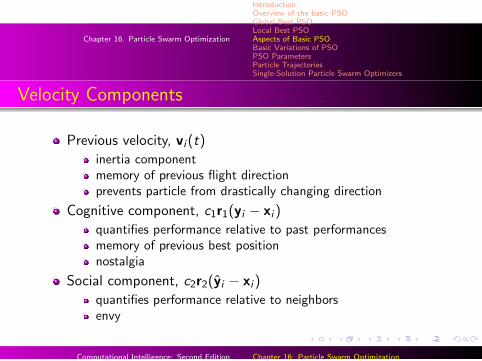
Velocity Components
Previous velocity, vi (t)
inertia componentmemory of previous flight directionprevents particle from drastically changing direction
Cognitive component, c1r1(yi − xi )
quantifies performance relative to past performancesmemory of previous best positionnostalgia
Social component, c2r2(yi − xi )
quantifies performance relative to neighborsenvy
Computational Intelligence: Second Edition Chapter 16: Particle Swarm Optimization
Chapter 16. Particle Swarm Optimization
IntroductionOverview of the basic PSOGlobal Best PSOLocal Best PSOAspects of Basic PSOBasic Variations of PSOPSO ParametersParticle TrajectoriesSingle-Solution Particle Swarm Optimizers
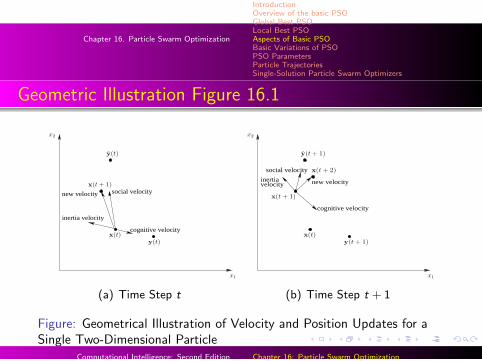
Geometric Illustration Figure 16.1
social velocity
cognitive velocity
inertia velocity
new velocity
x(t)y(t)
x(t + 1)
y(t)
x1
x2
(a) Time Step t
new velocity
cognitive velocity
social velocity
inertiavelocity
x(t)
y(t + 1)
x1
x2
y(t + 1)
x(t + 1)
x(t + 2)
(b) Time Step t + 1
Figure: Geometrical Illustration of Velocity and Position Updates for aSingle Two-Dimensional Particle
Computational Intelligence: Second Edition Chapter 16: Particle Swarm Optimization

Chapter 16. Particle Swarm Optimization
IntroductionOverview of the basic PSOGlobal Best PSOLocal Best PSOAspects of Basic PSOBasic Variations of PSOPSO ParametersParticle TrajectoriesSingle-Solution Particle Swarm Optimizers
Cumulative Effect of Position Updates (Figure 16.2)
x2
x1
y
(a) Time Step t
x2
x1
y
(b) Time Step t + 1
Figure: Multi-particle gbest PSO Illustration
Computational Intelligence: Second Edition Chapter 16: Particle Swarm Optimization
Chapter 16. Particle Swarm Optimization
IntroductionOverview of the basic PSOGlobal Best PSOLocal Best PSOAspects of Basic PSOBasic Variations of PSOPSO ParametersParticle TrajectoriesSingle-Solution Particle Swarm Optimizers
Stopping Conditions
Terminate when a maximum number of iterations, or FEs, hasbeen exceeded
Terminate when an acceptable solution has been found, i.e.when (assuming minimization)
f (xi ) ≤ |f (x∗)− ε|
Terminate when no improvement is observed over a number ofiterations
Computational Intelligence: Second Edition Chapter 16: Particle Swarm Optimization

Chapter 16. Particle Swarm Optimization
IntroductionOverview of the basic PSOGlobal Best PSOLocal Best PSOAspects of Basic PSOBasic Variations of PSOPSO ParametersParticle TrajectoriesSingle-Solution Particle Swarm Optimizers
Stopping Conditions (cont)
Terminate when the normalized swarm radius is close to zero,i.e.
Rnorm =Rmax
diameter(S(0))≈ 0
whereRmax = ||xm − y||, m = 1, . . . , ns
with||xm − y|| ≥ ||xi − y||, ∀i = 1, . . . , ns
Terminate when the objective function slope is approximatelyzero, i.e.
f′(t) =
f (y(t))− f (y(t − 1))
f (y(t))≈ 0
Computational Intelligence: Second Edition Chapter 16: Particle Swarm Optimization

Chapter 16. Particle Swarm Optimization
IntroductionOverview of the basic PSOGlobal Best PSOLocal Best PSOAspects of Basic PSOBasic Variations of PSOPSO ParametersParticle TrajectoriesSingle-Solution Particle Swarm Optimizers
Basic PSO Variations: Introduction
Main objectives of these variations are to improve
Convergence speedQuality of solutionsAbility to converge
Computational Intelligence: Second Edition Chapter 16: Particle Swarm Optimization

Chapter 16. Particle Swarm Optimization
IntroductionOverview of the basic PSOGlobal Best PSOLocal Best PSOAspects of Basic PSOBasic Variations of PSOPSO ParametersParticle TrajectoriesSingle-Solution Particle Swarm Optimizers
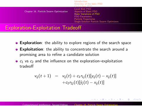
Exploration-Exploitation Tradeoff
Exploration: the ability to explore regions of the search space
Exploitation: the ability to concentrate the search around apromising area to refine a candidate solution
c1 vs c2 and the influence on the exploration–exploitationtradeoff
vij(t + 1) = vij(t) + c1r1j(t)[yij(t)− xij(t)]
+c2r2j(t)[yj(t)− xij(t)]
Computational Intelligence: Second Edition Chapter 16: Particle Swarm Optimization
Chapter 16. Particle Swarm Optimization
IntroductionOverview of the basic PSOGlobal Best PSOLocal Best PSOAspects of Basic PSOBasic Variations of PSOPSO ParametersParticle TrajectoriesSingle-Solution Particle Swarm Optimizers
Exploration-Exploitation Tradeoff
Exploration: the ability to explore regions of the search space
Exploitation: the ability to concentrate the search around apromising area to refine a candidate solution
c1 vs c2 and the influence on the exploration–exploitationtradeoff
vij(t + 1) = vij(t) + c1r1j(t)[yij(t)− xij(t)]
+c2r2j(t)[yj(t)− xij(t)]
Computational Intelligence: Second Edition Chapter 16: Particle Swarm Optimization

Chapter 16. Particle Swarm Optimization
IntroductionOverview of the basic PSOGlobal Best PSOLocal Best PSOAspects of Basic PSOBasic Variations of PSOPSO ParametersParticle TrajectoriesSingle-Solution Particle Swarm Optimizers
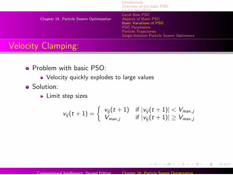
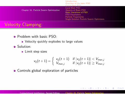
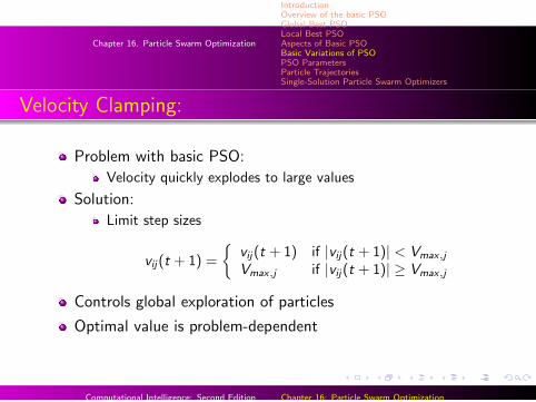
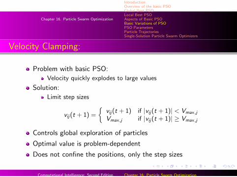
Velocity Clamping:
Problem with basic PSO:
Velocity quickly explodes to large values
Solution:
Limit step sizes
vij(t + 1) =
{vij(t + 1) if |vij(t + 1)| < Vmax,j
Vmax,j if |vij(t + 1)| ≥ Vmax,j
Controls global exploration of particles
Optimal value is problem-dependent
Does not confine the positions, only the step sizes
Computational Intelligence: Second Edition Chapter 16: Particle Swarm Optimization
Chapter 16. Particle Swarm Optimization
IntroductionOverview of the basic PSOGlobal Best PSOLocal Best PSOAspects of Basic PSOBasic Variations of PSOPSO ParametersParticle TrajectoriesSingle-Solution Particle Swarm Optimizers
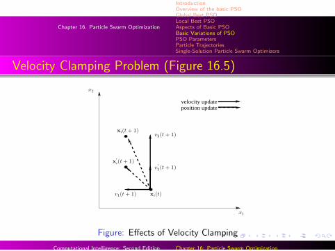
Velocity Clamping Problem (Figure 16.5)
position updatevelocity update
x1
v2(t + 1)
v1(t + 1) xi(t)
v′
2(t + 1)
x
′
i(t + 1)
xi(t + 1)
x2
Figure: Effects of Velocity Clamping
Computational Intelligence: Second Edition Chapter 16: Particle Swarm Optimization
Chapter 16. Particle Swarm Optimization
IntroductionOverview of the basic PSOGlobal Best PSOLocal Best PSOAspects of Basic PSOBasic Variations of PSOPSO ParametersParticle TrajectoriesSingle-Solution Particle Swarm Optimizers
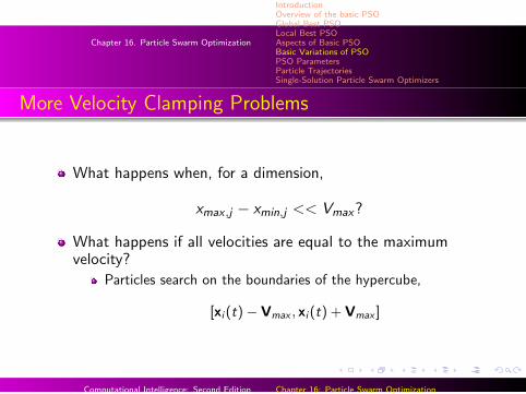
More Velocity Clamping Problems
What happens when, for a dimension,
xmax ,j − xmin,j << Vmax?
What happens if all velocities are equal to the maximumvelocity?
Particles search on the boundaries of the hypercube,
[xi (t)− Vmax , xi (t) + Vmax ]
Computational Intelligence: Second Edition Chapter 16: Particle Swarm Optimization
Chapter 16. Particle Swarm Optimization
IntroductionOverview of the basic PSOGlobal Best PSOLocal Best PSOAspects of Basic PSOBasic Variations of PSOPSO ParametersParticle TrajectoriesSingle-Solution Particle Swarm Optimizers
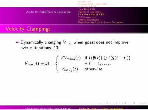
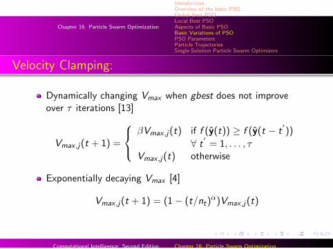
Velocity Clamping:
Dynamically changing Vmax when gbest does not improveover τ iterations [13]
Vmax ,j(t + 1) =
βVmax ,j(t) if f (y(t)) ≥ f (y(t − t
′))
∀ t′= 1, . . . , τ
Vmax ,j(t) otherwise
Exponentially decaying Vmax [4]
Vmax ,j(t + 1) = (1− (t/nt)α)Vmax ,j(t)
Computational Intelligence: Second Edition Chapter 16: Particle Swarm Optimization
Chapter 16. Particle Swarm Optimization
IntroductionOverview of the basic PSOGlobal Best PSOLocal Best PSOAspects of Basic PSOBasic Variations of PSOPSO ParametersParticle TrajectoriesSingle-Solution Particle Swarm Optimizers
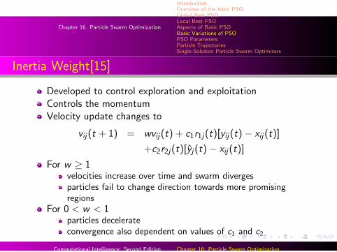
Inertia Weight[15]
Developed to control exploration and exploitationControls the momentumVelocity update changes to
vij(t + 1) = wvij(t) + c1r1j(t)[yij(t)− xij(t)]
+c2r2j(t)[yj(t)− xij(t)]
For w ≥ 1velocities increase over time and swarm divergesparticles fail to change direction towards more promisingregions
For 0 < w < 1particles decelerateconvergence also dependent on values of c1 and c2
Computational Intelligence: Second Edition Chapter 16: Particle Swarm Optimization
Chapter 16. Particle Swarm Optimization
IntroductionOverview of the basic PSOGlobal Best PSOLocal Best PSOAspects of Basic PSOBasic Variations of PSOPSO ParametersParticle TrajectoriesSingle-Solution Particle Swarm Optimizers
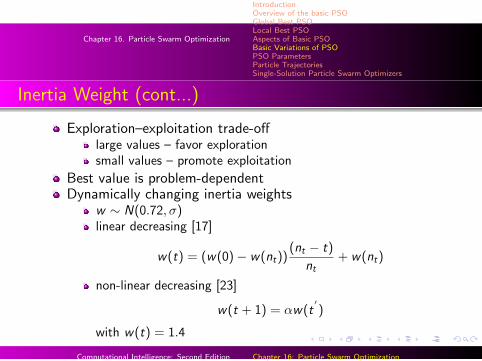
Inertia Weight (cont...)
Exploration–exploitation trade-offlarge values – favor explorationsmall values – promote exploitation
Best value is problem-dependent
Dynamically changing inertia weightsw ∼ N(0.72, σ)linear decreasing [17]
w(t) = (w(0)− w(nt))(nt − t)
nt+ w(nt)
non-linear decreasing [23]
w(t + 1) = αw(t′)
with w(t) = 1.4
Computational Intelligence: Second Edition Chapter 16: Particle Swarm Optimization
Chapter 16. Particle Swarm Optimization
IntroductionOverview of the basic PSOGlobal Best PSOLocal Best PSOAspects of Basic PSOBasic Variations of PSOPSO ParametersParticle TrajectoriesSingle-Solution Particle Swarm Optimizers
Inertia Weight (cont...)
Exploration–exploitation trade-offlarge values – favor explorationsmall values – promote exploitation
Best value is problem-dependentDynamically changing inertia weights
w ∼ N(0.72, σ)linear decreasing [17]
w(t) = (w(0)− w(nt))(nt − t)
nt+ w(nt)
non-linear decreasing [23]
w(t + 1) = αw(t′)
with w(t) = 1.4
Computational Intelligence: Second Edition Chapter 16: Particle Swarm Optimization

Chapter 16. Particle Swarm Optimization
IntroductionOverview of the basic PSOGlobal Best PSOLocal Best PSOAspects of Basic PSOBasic Variations of PSOPSO ParametersParticle TrajectoriesSingle-Solution Particle Swarm Optimizers
Constriction Coefficient [2]
Developed to ensure convergence to a stable point withoutthe need for velocity clamping
vij(t + 1) = χ[vij(t) + φ1(yij(t)− xij(t))
+φ2(yj(t)− xij(t))]
where
χ =2κ
|2− φ−√
φ(φ− 4)|with
φ = φ1 + φ2
φ1 = c1r1, φ2 = c2r2
Computational Intelligence: Second Edition Chapter 16: Particle Swarm Optimization
Chapter 16. Particle Swarm Optimization
IntroductionOverview of the basic PSOGlobal Best PSOLocal Best PSOAspects of Basic PSOBasic Variations of PSOPSO ParametersParticle TrajectoriesSingle-Solution Particle Swarm Optimizers
Constriction Coefficient (cont...)
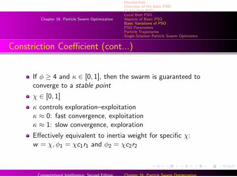
If φ ≥ 4 and κ ∈ [0, 1], then the swarm is guaranteed toconverge to a stable point
χ ∈ [0, 1]
κ controls exploration–exploitationκ ≈ 0: fast convergence, exploitationκ ≈ 1: slow convergence, exploration
Effectively equivalent to inertia weight for specific χ:w = χ, φ1 = χc1r1 and φ2 = χc2r2
Computational Intelligence: Second Edition Chapter 16: Particle Swarm Optimization
Chapter 16. Particle Swarm Optimization
IntroductionOverview of the basic PSOGlobal Best PSOLocal Best PSOAspects of Basic PSOBasic Variations of PSOPSO ParametersParticle TrajectoriesSingle-Solution Particle Swarm Optimizers
Synchronous vs asynchronous updates
Synchronous:
Personal best and neighborhood bests updated separately fromposition and velocity vectorsslower feedbackbetter for gbest
Asynchronous:
new best positions updated after each particle position updateimmediate feedback about best regions of the search spacebetter for lbest
Computational Intelligence: Second Edition Chapter 16: Particle Swarm Optimization
Chapter 16. Particle Swarm Optimization
IntroductionOverview of the basic PSOGlobal Best PSOLocal Best PSOAspects of Basic PSOBasic Variations of PSOPSO ParametersParticle TrajectoriesSingle-Solution Particle Swarm Optimizers
Velocity Models
Cognition-only model:
vij(t + 1) = vij(t) + c1r1j(t)(yij(t)− xij(t))
particles are independent hill-climberslocal search by each particle
Social-only model:
vij(t + 1) = vij(t) + c2r2j(t)(yj(t)− xij(t))
swarm is one stochastic hill-climberSelfless model:
Social model, but nbest solution chosen from neighbors onlyParticle itself is not allowed to become the nbest
Computational Intelligence: Second Edition Chapter 16: Particle Swarm Optimization
Chapter 16. Particle Swarm Optimization
IntroductionOverview of the basic PSOGlobal Best PSOLocal Best PSOAspects of Basic PSOBasic Variations of PSOPSO ParametersParticle TrajectoriesSingle-Solution Particle Swarm Optimizers
Basic Parameters
Swarm size, ns
Particle dimension, nx
Neighborhood size, nNi
Number of iterations, nt
Inertia weight, w
Acceleration coefficients, c1 and c2
Computational Intelligence: Second Edition Chapter 16: Particle Swarm Optimization
Chapter 16. Particle Swarm Optimization
IntroductionOverview of the basic PSOGlobal Best PSOLocal Best PSOAspects of Basic PSOBasic Variations of PSOPSO ParametersParticle TrajectoriesSingle-Solution Particle Swarm Optimizers
Acceleration Coefficients
c1 = c2 = 0?
c1 > 0, c2 = 0: cognition-only model
c1 = 0, c2 > 0: social-only model
c1 = c2 > 0:
particles are attracted towards the average of yi and yi
c2 > c1:
more beneficial for unimodal problems
Computational Intelligence: Second Edition Chapter 16: Particle Swarm Optimization
Chapter 16. Particle Swarm Optimization
IntroductionOverview of the basic PSOGlobal Best PSOLocal Best PSOAspects of Basic PSOBasic Variations of PSOPSO ParametersParticle TrajectoriesSingle-Solution Particle Swarm Optimizers
Acceleration Coefficients (cont)
c1 < c2:more beneficial for multimodal problems
Low c1 and c2:smooth particle trajectories
High c1 and c2:more acceleration, abrupt movements
Adaptive acceleration coefficients
c1(t) = (c1,min − c1,max)t
nt+ c1,max
c2(t) = (c2,max − c2,min)t
nt+ c2,min
Computational Intelligence: Second Edition Chapter 16: Particle Swarm Optimization

Chapter 16. Particle Swarm Optimization
IntroductionOverview of the basic PSOGlobal Best PSOLocal Best PSOAspects of Basic PSOBasic Variations of PSOPSO ParametersParticle TrajectoriesSingle-Solution Particle Swarm Optimizers
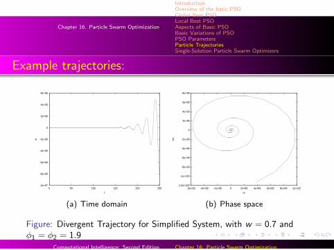
Simplified Particle Trajectories [19, 22]
No stochastic component
Single, one-dimensional particle
Using w
Personal best and global best are fixed:y = 1.0, y = 0.0
φ1 = c1r1 and φ2 = c2r2
Computational Intelligence: Second Edition Chapter 16: Particle Swarm Optimization
Chapter 16. Particle Swarm Optimization
IntroductionOverview of the basic PSOGlobal Best PSOLocal Best PSOAspects of Basic PSOBasic Variations of PSOPSO ParametersParticle TrajectoriesSingle-Solution Particle Swarm Optimizers
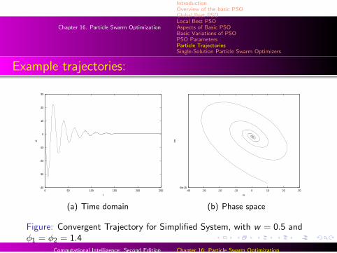
Example trajectories:
-40
-30
-20
-10
0
10
20
30
0 50 100 150 200 250
xt
t
(a) Time domain
-6e-16-40 -30 -20 -10 0 10 20 30
im
re
(b) Phase space
Figure: Convergent Trajectory for Simplified System, with w = 0.5 andφ1 = φ2 = 1.4
Computational Intelligence: Second Edition Chapter 16: Particle Swarm Optimization

Chapter 16. Particle Swarm Optimization
IntroductionOverview of the basic PSOGlobal Best PSOLocal Best PSOAspects of Basic PSOBasic Variations of PSOPSO ParametersParticle TrajectoriesSingle-Solution Particle Swarm Optimizers
Example trajectories:
-500
-400
-300
-200
-100
0
100
200
300
400
500
0 50 100 150 200 250
xt
t
(a) Time domain
-6e-16-500 -400 -300 -200 -100 0 100 200 300 400 500
im
re
(b) Phase space
Figure: Cyclic Trajectory for Simplified System, with w = 1.0 andφ1 = φ2 = 1.999
Computational Intelligence: Second Edition Chapter 16: Particle Swarm Optimization
Chapter 16. Particle Swarm Optimization
IntroductionOverview of the basic PSOGlobal Best PSOLocal Best PSOAspects of Basic PSOBasic Variations of PSOPSO ParametersParticle TrajectoriesSingle-Solution Particle Swarm Optimizers
Example trajectories:
-1e+07
-8e+06
-6e+06
-4e+06
-2e+06
0
2e+06
4e+06
6e+06
0 50 100 150 200 250
xt
t
(a) Time domain
-1.2e+100
-1e+100
-8e+99
-6e+99
-4e+99
-2e+99
0
2e+99
4e+99
6e+99
8e+99
-6e+99 -4e+99 -2e+99 0 2e+99 4e+99 6e+99 8e+99 1e+100
im
re
(b) Phase space
Figure: Divergent Trajectory for Simplified System, with w = 0.7 andφ1 = φ2 = 1.9
Computational Intelligence: Second Edition Chapter 16: Particle Swarm Optimization

Chapter 16. Particle Swarm Optimization
IntroductionOverview of the basic PSOGlobal Best PSOLocal Best PSOAspects of Basic PSOBasic Variations of PSOPSO ParametersParticle TrajectoriesSingle-Solution Particle Swarm Optimizers
Convergence Conditions:
What do we mean by the term convergence?
0 4.0
1
2.0z1phi
wz2
Figure: Convergence Map for Values of w and φ = φ1 + φ2
Computational Intelligence: Second Edition Chapter 16: Particle Swarm Optimization
Chapter 16. Particle Swarm Optimization
IntroductionOverview of the basic PSOGlobal Best PSOLocal Best PSOAspects of Basic PSOBasic Variations of PSOPSO ParametersParticle TrajectoriesSingle-Solution Particle Swarm Optimizers
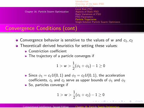
Convergence Conditions (cont)
Convergence behavior is sensitive to the values of w and c1, c2
Theoreticall derived heuristics for setting these values:Constriction coefficientThe trajectory of a particle converges if
1 > w >1
2(φ1 + φ2)− 1 ≥ 0
Since φ1 = c1U(0, 1) and φ2 = c2U(0, 1), the accelerationcoefficients, c1 and c2 serve as upper bounds of φ1 and φ2
So, particles converge if
1 > w >1
2(c1 + c2)− 1 ≥ 0
Computational Intelligence: Second Edition Chapter 16: Particle Swarm Optimization

Chapter 16. Particle Swarm Optimization
IntroductionOverview of the basic PSOGlobal Best PSOLocal Best PSOAspects of Basic PSOBasic Variations of PSOPSO ParametersParticle TrajectoriesSingle-Solution Particle Swarm Optimizers
Convergence Conditions (cont)
It can happen that, for stochastic φ1 and φ2 and a w that violatesthe condition above, the swarm may still converge
-30
-20
-10
0
10
20
30
40
0 50 100 150 200 250
x(t)
t
Figure: Stochastic Particle Trajectory for w = 0.9 and c1 = c2 = 2.0
Computational Intelligence: Second Edition Chapter 16: Particle Swarm Optimization

Chapter 16. Particle Swarm Optimization
IntroductionOverview of the basic PSOGlobal Best PSOLocal Best PSOAspects of Basic PSOBasic Variations of PSOPSO ParametersParticle TrajectoriesSingle-Solution Particle Swarm Optimizers
Guaranteed Convergence PSO
For the basic PSO, what happens when
xi = yi = y
and if this condition persists for a number of iterations?
The problem:wvi → 0
which leads to stagnation, where particles have converged onthe best position found by the swarm
Computational Intelligence: Second Edition Chapter 16: Particle Swarm Optimization
Chapter 16. Particle Swarm Optimization
IntroductionOverview of the basic PSOGlobal Best PSOLocal Best PSOAspects of Basic PSOBasic Variations of PSOPSO ParametersParticle TrajectoriesSingle-Solution Particle Swarm Optimizers
Guaranteed Convergence PSO (cont)
How can we address this problem?
Force the global best position to change when
xi = yi = y
This is what happens in the GCPSO, where the global bestparticle is forced to search in a bounding box around thecurrent position for a better position
Computational Intelligence: Second Edition Chapter 16: Particle Swarm Optimization
Chapter 16. Particle Swarm Optimization
IntroductionOverview of the basic PSOGlobal Best PSOLocal Best PSOAspects of Basic PSOBasic Variations of PSOPSO ParametersParticle TrajectoriesSingle-Solution Particle Swarm Optimizers
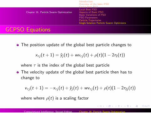
GCPSO Equations
The position update of the global best particle changes to
xτ j(t + 1) = yj(t) + wvτ j(t) + ρ(t)(1− 2r2(t))
where τ is the index of the global best particle
The velocity update of the global best particle then has tochange to
vτ j(t + 1) = −xτ j(t) + yj(t) + wvτ j(t) + ρ(t)(1− 2r2j(t))
where where ρ(t) is a scaling factor
Computational Intelligence: Second Edition Chapter 16: Particle Swarm Optimization
Chapter 16. Particle Swarm Optimization
IntroductionOverview of the basic PSOGlobal Best PSOLocal Best PSOAspects of Basic PSOBasic Variations of PSOPSO ParametersParticle TrajectoriesSingle-Solution Particle Swarm Optimizers
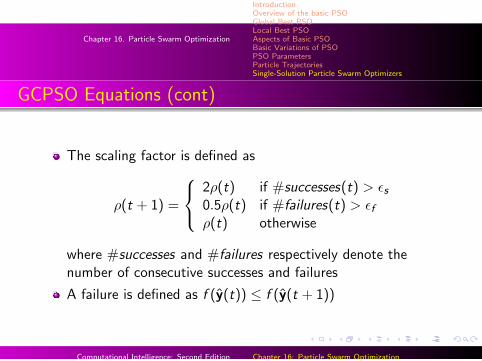
GCPSO Equations (cont)
The scaling factor is defined as
ρ(t + 1) =
2ρ(t) if #successes(t) > εs0.5ρ(t) if #failures(t) > εfρ(t) otherwise
where #successes and #failures respectively denote thenumber of consecutive successes and failures
A failure is defined as f (y(t)) ≤ f (y(t + 1))
Computational Intelligence: Second Edition Chapter 16: Particle Swarm Optimization

Chapter 16. Particle Swarm Optimization
IntroductionOverview of the basic PSOGlobal Best PSOLocal Best PSOAspects of Basic PSOBasic Variations of PSOPSO ParametersParticle TrajectoriesSingle-Solution Particle Swarm Optimizers
Social-Based Particle Swarm Optimization
Spatial neighborhoods
Fitness-Based spatial neighborhoods
Growing neighborhoods
Hypercube structure
Fully informed PSO
Barebones PSO
Computational Intelligence: Second Edition Chapter 16: Particle Swarm Optimization
Chapter 16. Particle Swarm Optimization
IntroductionOverview of the basic PSOGlobal Best PSOLocal Best PSOAspects of Basic PSOBasic Variations of PSOPSO ParametersParticle TrajectoriesSingle-Solution Particle Swarm Optimizers
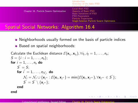
Spatial Social Networks: Algorithm 16.4
Neighborhoods usually formed on the basis of particle indices
Based on spatial neighborhoods:
Calculate the Euclidean distance E(xi1 , xi2),∀i1, i2 = 1, . . . , ns ;S = {i : i = 1, . . . , ns};for i = 1, . . . , ns do
S′= S ;
for i′= 1, . . . , nN
i′ do
Ni = Ni ∪ {xi ′′ : E(xi , xi ′′ ) = min{E(xi , xi ′′′ ),∀xi ′′′ ∈ S′};
S′= S
′ \ {xi ′′};end
end
Computational Intelligence: Second Edition Chapter 16: Particle Swarm Optimization
Chapter 16. Particle Swarm Optimization
IntroductionOverview of the basic PSOGlobal Best PSOLocal Best PSOAspects of Basic PSOBasic Variations of PSOPSO ParametersParticle TrajectoriesSingle-Solution Particle Swarm Optimizers
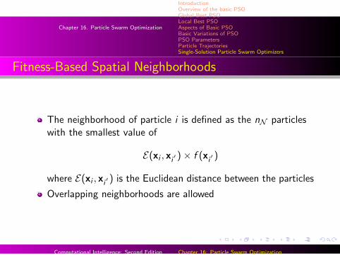
Fitness-Based Spatial Neighborhoods
The neighborhood of particle i is defined as the nN particleswith the smallest value of
E(xi , xi ′ )× f (xi ′ )
where E(xi , xi ′ ) is the Euclidean distance between the particles
Overlapping neighborhoods are allowed
Computational Intelligence: Second Edition Chapter 16: Particle Swarm Optimization
Chapter 16. Particle Swarm Optimization
IntroductionOverview of the basic PSOGlobal Best PSOLocal Best PSOAspects of Basic PSOBasic Variations of PSOPSO ParametersParticle TrajectoriesSingle-Solution Particle Swarm Optimizers
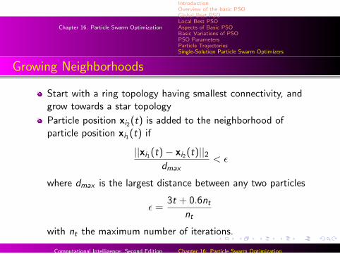
Growing Neighborhoods
Start with a ring topology having smallest connectivity, andgrow towards a star topology
Particle position xi2(t) is added to the neighborhood ofparticle position xi1(t) if
||xi1(t)− xi2(t)||2dmax
< ε
where dmax is the largest distance between any two particles
ε =3t + 0.6nt
nt
with nt the maximum number of iterations.
Computational Intelligence: Second Edition Chapter 16: Particle Swarm Optimization
Chapter 16. Particle Swarm Optimization
IntroductionOverview of the basic PSOGlobal Best PSOLocal Best PSOAspects of Basic PSOBasic Variations of PSOPSO ParametersParticle TrajectoriesSingle-Solution Particle Swarm Optimizers
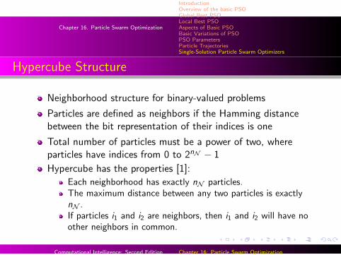
Hypercube Structure
Neighborhood structure for binary-valued problems
Particles are defined as neighbors if the Hamming distancebetween the bit representation of their indices is one
Total number of particles must be a power of two, whereparticles have indices from 0 to 2nN − 1
Hypercube has the properties [1]:
Each neighborhood has exactly nN particles.The maximum distance between any two particles is exactlynN .If particles i1 and i2 are neighbors, then i1 and i2 will have noother neighbors in common.
Computational Intelligence: Second Edition Chapter 16: Particle Swarm Optimization
Chapter 16. Particle Swarm Optimization
IntroductionOverview of the basic PSOGlobal Best PSOLocal Best PSOAspects of Basic PSOBasic Variations of PSOPSO ParametersParticle TrajectoriesSingle-Solution Particle Swarm Optimizers
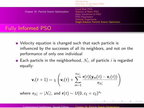
Fully Informed PSO
Velocity equation is changed such that each particle isinfluenced by the successes of all its neighbors, and not on theperformance of only one individual
Each particle in the neighborhood, Ni , of particle i is regardedequally:
vi (t + 1) = χ
(vi (t) +
nNi∑m=1
r(t)(ym(t)− xi (t))
nNi
)
where nNi= |Ni |, and r(t) ∼ U(0, c1 + c2)
nx
Computational Intelligence: Second Edition Chapter 16: Particle Swarm Optimization
Chapter 16. Particle Swarm Optimization
IntroductionOverview of the basic PSOGlobal Best PSOLocal Best PSOAspects of Basic PSOBasic Variations of PSOPSO ParametersParticle TrajectoriesSingle-Solution Particle Swarm Optimizers
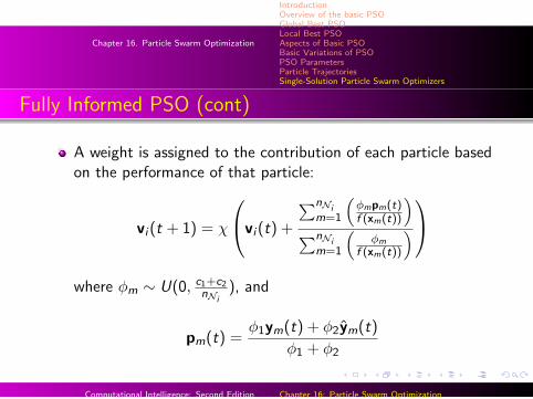
Fully Informed PSO (cont)
A weight is assigned to the contribution of each particle basedon the performance of that particle:
vi (t + 1) = χ
vi (t) +
∑nNim=1
(φmpm(t)f (xm(t))
)∑nNi
m=1
(φm
f (xm(t))
)
where φm ∼ U(0, c1+c2nNi
), and
pm(t) =φ1ym(t) + φ2ym(t)
φ1 + φ2
Computational Intelligence: Second Edition Chapter 16: Particle Swarm Optimization
Chapter 16. Particle Swarm Optimization
IntroductionOverview of the basic PSOGlobal Best PSOLocal Best PSOAspects of Basic PSOBasic Variations of PSOPSO ParametersParticle TrajectoriesSingle-Solution Particle Swarm Optimizers
Fully Informed PSO (cont)
Advantages:
More information is used to decide on the best direction toseachInfluence of a particle on the step size is proportional to theparticle’s fitness
Disadvantages
Influences of multiple particles may cancel each otherWhat happens when all particles are positioned symmetricallyaround the particle being updated?
Computational Intelligence: Second Edition Chapter 16: Particle Swarm Optimization
Chapter 16. Particle Swarm Optimization
IntroductionOverview of the basic PSOGlobal Best PSOLocal Best PSOAspects of Basic PSOBasic Variations of PSOPSO ParametersParticle TrajectoriesSingle-Solution Particle Swarm Optimizers
Barebones PSO
Formal proofs [18, 19, 22] have shown that each particleconverges to a point that is a weighted average between thepersonal best and neighborhood best positions:
yij(t) + yij(t)
2
This behavior supports Kennedy’s proposal to replace theentire velocity by
vij(t + 1) ∼ N
(yij(t) + yij(t)
2, σ
)where
σ = |yij(t)− yij(t)|
Computational Intelligence: Second Edition Chapter 16: Particle Swarm Optimization
Chapter 16. Particle Swarm Optimization
IntroductionOverview of the basic PSOGlobal Best PSOLocal Best PSOAspects of Basic PSOBasic Variations of PSOPSO ParametersParticle TrajectoriesSingle-Solution Particle Swarm Optimizers
Barebones PSO (cont)
The position update is simply
xij(t + 1) = vij(t + 1)
Alternative formulation:
vij(t + 1) =
{yij(t) if U(0, 1) < 0.5
N(yij (t)+yij (t)
2 , σ) otherwise
There is a 50% chance that the j-th dimension of the particledimension changes to the corresponding personal best position
Computational Intelligence: Second Edition Chapter 16: Particle Swarm Optimization
Chapter 16. Particle Swarm Optimization
IntroductionOverview of the basic PSOGlobal Best PSOLocal Best PSOAspects of Basic PSOBasic Variations of PSOPSO ParametersParticle TrajectoriesSingle-Solution Particle Swarm Optimizers
Hybrid Algorithms
Selection-based PSO
Reproduction in PSO
Mutation in PSO
Differential evolution based PSO
Computational Intelligence: Second Edition Chapter 16: Particle Swarm Optimization
Chapter 16. Particle Swarm Optimization
IntroductionOverview of the basic PSOGlobal Best PSOLocal Best PSOAspects of Basic PSOBasic Variations of PSOPSO ParametersParticle TrajectoriesSingle-Solution Particle Swarm Optimizers
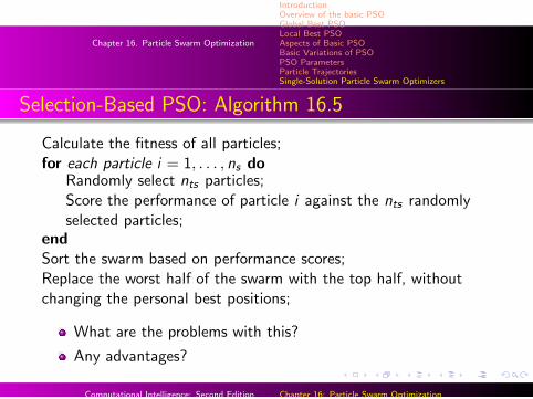
Selection-Based PSO: Algorithm 16.5
Calculate the fitness of all particles;for each particle i = 1, . . . , ns do
Randomly select nts particles;Score the performance of particle i against the nts randomlyselected particles;
endSort the swarm based on performance scores;Replace the worst half of the swarm with the top half, withoutchanging the personal best positions;
What are the problems with this?
Any advantages?
Computational Intelligence: Second Edition Chapter 16: Particle Swarm Optimization
Chapter 16. Particle Swarm Optimization
IntroductionOverview of the basic PSOGlobal Best PSOLocal Best PSOAspects of Basic PSOBasic Variations of PSOPSO ParametersParticle TrajectoriesSingle-Solution Particle Swarm Optimizers
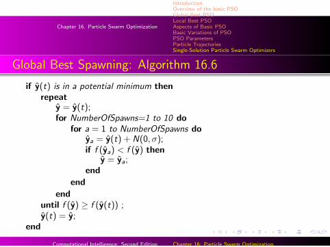
Global Best Spawning: Algorithm 16.6
if y(t) is in a potential minimum thenrepeat
y = y(t);for NumberOfSpawns=1 to 10 do
for a = 1 to NumberOfSpawns doya = y(t) + N(0, σ);if f (ya) < f (y) then
y = ya;end
end
enduntil f (y) ≥ f (y(t)) ;y(t) = y;
end
Computational Intelligence: Second Edition Chapter 16: Particle Swarm Optimization
Chapter 16. Particle Swarm Optimization
IntroductionOverview of the basic PSOGlobal Best PSOLocal Best PSOAspects of Basic PSOBasic Variations of PSOPSO ParametersParticle TrajectoriesSingle-Solution Particle Swarm Optimizers
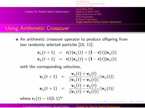
Using Arithmetic Crossover
An arithmetic crossover operator to produce offspring fromtwo randomly selected particles [10, 11]:
xi1(t + 1) = r(t)xi1(t) + (1− r(t))xi2(t)
xi2(t + 1) = r(t)xi2(t) + (1− r(t))xi1(t)
with the corresponding velocities,
vi1(t + 1) =vi1(t) + vi2(t)
||vi1(t) + vi2(t)||||vi1(t)||
vi2(t + 1) =vi1(t) + vi2(t)
||vi1(t) + vi2(t)||||vi2(t)||
where r1(t) ∼ U(0, 1)nx
Computational Intelligence: Second Edition Chapter 16: Particle Swarm Optimization

Chapter 16. Particle Swarm Optimization
IntroductionOverview of the basic PSOGlobal Best PSOLocal Best PSOAspects of Basic PSOBasic Variations of PSOPSO ParametersParticle TrajectoriesSingle-Solution Particle Swarm Optimizers
Using Arithmetic Crossover (cont)
Personal best position of an offspring is initialized to itscurrent position:
yi1(t + 1) = xi1(t + 1)
Particles are selected for breeding at a user-specified breedingprobability
Random selection of parents prevents the best particles fromdominating the breeding process
Breeding process is done for each iteration after the velocityand position updates have been done
Computational Intelligence: Second Edition Chapter 16: Particle Swarm Optimization
Chapter 16. Particle Swarm Optimization
IntroductionOverview of the basic PSOGlobal Best PSOLocal Best PSOAspects of Basic PSOBasic Variations of PSOPSO ParametersParticle TrajectoriesSingle-Solution Particle Swarm Optimizers
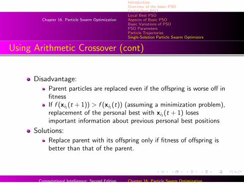
Using Arithmetic Crossover (cont)
Disadvantage:
Parent particles are replaced even if the offspring is worse off infitnessIf f (xi1(t + 1)) > f (xi1(t)) (assuming a minimization problem),replacement of the personal best with xi1(t + 1) losesimportant information about previous personal best positions
Solutions:
Replace parent with its offspring only if fitness of offspring isbetter than that of the parent.
Computational Intelligence: Second Edition Chapter 16: Particle Swarm Optimization
Chapter 16. Particle Swarm Optimization
IntroductionOverview of the basic PSOGlobal Best PSOLocal Best PSOAspects of Basic PSOBasic Variations of PSOPSO ParametersParticle TrajectoriesSingle-Solution Particle Swarm Optimizers
Mutation PSO
Mutate the global best position:
y(t + 1) = y′(t + 1) + η
′N(0, 1)
where y′(t + 1) represents the unmutated global best position,
and η′is referred to as a learning parameter
Mutate the componets of position vectors: For each j , ifU(0, 1) < Pm, then component x
′ij(t + 1) is mutated using [6]
xij(t + 1) = x′ij(t + 1) + N(0, σ)x
′ij(t + 1)
whereσ = 0.1(xmax ,j − xmin,j)
Computational Intelligence: Second Edition Chapter 16: Particle Swarm Optimization

Chapter 16. Particle Swarm Optimization
IntroductionOverview of the basic PSOGlobal Best PSOLocal Best PSOAspects of Basic PSOBasic Variations of PSOPSO ParametersParticle TrajectoriesSingle-Solution Particle Swarm Optimizers
Mutation PSO (cont)
Each xij can have its own deviation:
σij(t) = σij(t − 1) eτ′N(0,1)+τNj (0,1)
with
τ′
=1√
2√
nx
τ =1√2nx
Computational Intelligence: Second Edition Chapter 16: Particle Swarm Optimization

Chapter 16. Particle Swarm Optimization
IntroductionOverview of the basic PSOGlobal Best PSOLocal Best PSOAspects of Basic PSOBasic Variations of PSOPSO ParametersParticle TrajectoriesSingle-Solution Particle Swarm Optimizers
Mutation PSO (cont)
Secrest and Lamont [14] adjust particle positions as follows
xi (t + 1) =
{yi (t) + vi (t + 1) if U(0, 1) > c1
y(t) + vi (t + 1) otherwise
wherevi (t + 1) = |vi (t + 1)|rθ
rθ is a random vector with magnitude of one and angleuniformly distributed from 0 to 2π and
vi (t+1)| ={
N(0, (1− c2)||yi (t)− y(t)||2) if U(0, 1) > c1
N(0, c2||yi (t)− y(t)||2) otherwise
Computational Intelligence: Second Edition Chapter 16: Particle Swarm Optimization
Chapter 16. Particle Swarm Optimization
IntroductionOverview of the basic PSOGlobal Best PSOLocal Best PSOAspects of Basic PSOBasic Variations of PSOPSO ParametersParticle TrajectoriesSingle-Solution Particle Swarm Optimizers
Differential Evolution PSO
After the normal velocity and position updates,
Select x1(t) 6= x2(t) 6= x3(t)Compute offspring:
x′
ij(t + 1) =
x1j(t) + β(x2j(t)− x3j(t)) if U(0, 1) ≤ Pc
or j = U(1, nx)xij(t) otherwise
where Pc ∈ (0, 1) is the probability of crossover, and β > 0 isa scaling factorReplace position of the particle if the offspring is better, i.e.xi (t + 1) = x
′
i (t + 1) only if f (x′
i (t + 1)) < f (xi (t)), otherwisexi (t + 1) = xi (t)
Computational Intelligence: Second Edition Chapter 16: Particle Swarm Optimization
Chapter 16. Particle Swarm Optimization
IntroductionOverview of the basic PSOGlobal Best PSOLocal Best PSOAspects of Basic PSOBasic Variations of PSOPSO ParametersParticle TrajectoriesSingle-Solution Particle Swarm Optimizers
Differential Evolution PSO (cont)
Apply DE crossover on personal best positions only [24]:
y′ij(t + 1) =
{yij(t) + δj if U(0, 1) < Pc and j = U(1, nx)yij(t) otherwise
where δ is the general difference vector defined as,
δj =y1j(t)− y2j(t)
2
and y1j(t) and y2j(t) randomly selected personal bestpositions
yij(t + 1) is set to y′ij(t + 1) only if the new personal best has
a better fitness
Computational Intelligence: Second Edition Chapter 16: Particle Swarm Optimization
Chapter 16. Particle Swarm Optimization
IntroductionOverview of the basic PSOGlobal Best PSOLocal Best PSOAspects of Basic PSOBasic Variations of PSOPSO ParametersParticle TrajectoriesSingle-Solution Particle Swarm Optimizers
Sub-Swarm Based PSO
Cooperative Split PSO
Hybrid Cooperative Split PSO
Predator-Prey PSO
Life-cycle PSO
Attractive and Repulsive PSO
Computational Intelligence: Second Edition Chapter 16: Particle Swarm Optimization
Chapter 16. Particle Swarm Optimization
IntroductionOverview of the basic PSOGlobal Best PSOLocal Best PSOAspects of Basic PSOBasic Variations of PSOPSO ParametersParticle TrajectoriesSingle-Solution Particle Swarm Optimizers
Cooperative Split PSO
Each particle is split into K separate parts of smallerdimension [19, 20, 21]
Each part is then optimized using a separate sub-swarm
If K = nx , each dimension is optimized by a separatesub-swarm, using any PSO algorithm
What are the issues?
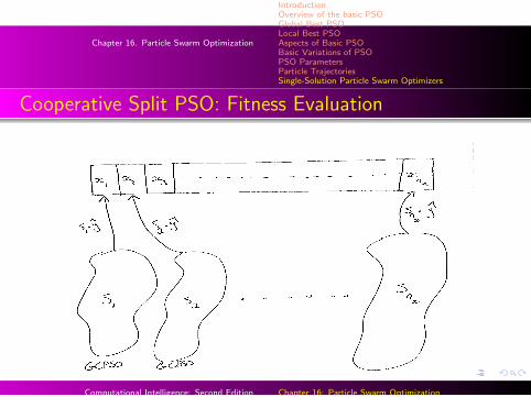
Problem if there are strong dependencies among variablesHow should the fitness of sub-swarm particles be evaluated?
Computational Intelligence: Second Edition Chapter 16: Particle Swarm Optimization
Chapter 16. Particle Swarm Optimization
IntroductionOverview of the basic PSOGlobal Best PSOLocal Best PSOAspects of Basic PSOBasic Variations of PSOPSO ParametersParticle TrajectoriesSingle-Solution Particle Swarm Optimizers
Cooperative Split PSO: Fitness Evaluation
Computational Intelligence: Second Edition Chapter 16: Particle Swarm Optimization
Chapter 16. Particle Swarm Optimization
IntroductionOverview of the basic PSOGlobal Best PSOLocal Best PSOAspects of Basic PSOBasic Variations of PSOPSO ParametersParticle TrajectoriesSingle-Solution Particle Swarm Optimizers
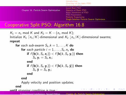
Cooperative Split PSO: Algorithm 16.8
K1 = nx mod K and K2 = K − (nx mod K );Initialize K1 dnx/Ke-dimensional and K2 bnx/Kc-dimensional swarms;repeat
for each sub-swarm Sk ,k = 1, . . . ,K dofor each particle i = 1, . . . ,Sk .ns do
if f (b(k,Sk .xi )) < f (b(k,Sk .yi )) thenSk .yi = Sk .xi ;
endif f (b(k,Sk .yi )) < f (b(k,Sk .y)) then
Sk .y = Sk .yi ;end
endApply velocity and position updates;
enduntil stopping condition is true ;
Computational Intelligence: Second Edition Chapter 16: Particle Swarm Optimization

Chapter 16. Particle Swarm Optimization
IntroductionOverview of the basic PSOGlobal Best PSOLocal Best PSOAspects of Basic PSOBasic Variations of PSOPSO ParametersParticle TrajectoriesSingle-Solution Particle Swarm Optimizers
Cooperative Split PSO (cont)
Advantages:
Instead of solving one large dimensional problem, severalsmaller dimensional problems are now solvedFitness function is evaluated after each subpart of the contextvector is updated, allowing a finer-grained searchImproved accuracies have been obtained for many optimizationproblems
Computational Intelligence: Second Edition Chapter 16: Particle Swarm Optimization

Chapter 16. Particle Swarm Optimization
IntroductionOverview of the basic PSOGlobal Best PSOLocal Best PSOAspects of Basic PSOBasic Variations of PSOPSO ParametersParticle TrajectoriesSingle-Solution Particle Swarm Optimizers
Hybrid Cooperative Split PSO
Hybrid Cooperative Split PSO:
Have subswarm and a main swarmMain swarm solves the complete problemAfter one iteration of the cooperative algoritihm, replace arandomly selected particle from the main swarm with thecontext vectorRandomly selected particle’s personal best should not be aneighborhood bestAfter a GCPSO update of the main swarm, replace a randomlyselected particle from each subswarm with the correspondingelement in the global best position of the main swarmRandomly selected subswarm particle’s personal best shouldnot be the global best for that particle.
Computational Intelligence: Second Edition Chapter 16: Particle Swarm Optimization
Chapter 16. Particle Swarm Optimization
IntroductionOverview of the basic PSOGlobal Best PSOLocal Best PSOAspects of Basic PSOBasic Variations of PSOPSO ParametersParticle TrajectoriesSingle-Solution Particle Swarm Optimizers
Predator-Prey PSO
Competition introduced to balance exploration–exploitationUses a second swarm of predator particles:
Prey particles scatter (explore) by being repelled by thepresence of predator particlesSilva et al. [16] use only one predator to pursue the global bestprey particleThe velocity update for the predator particle is defined as
vp(t + 1) = r(y(t)− xp(t))
where vp and xp are respectively the velocity and positionvectors of the predator particle, pr ∼ U(0,Vmax,p)
nx
Vmax,p controls the speed at which the predator catches thebest prey
Computational Intelligence: Second Edition Chapter 16: Particle Swarm Optimization
Chapter 16. Particle Swarm Optimization
IntroductionOverview of the basic PSOGlobal Best PSOLocal Best PSOAspects of Basic PSOBasic Variations of PSOPSO ParametersParticle TrajectoriesSingle-Solution Particle Swarm Optimizers
Predator-Prey PSO (cont)
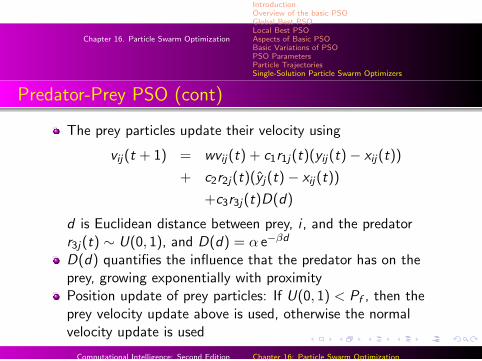
The prey particles update their velocity using
vij(t + 1) = wvij(t) + c1r1j(t)(yij(t)− xij(t))
+ c2r2j(t)(yj(t)− xij(t))
+c3r3j(t)D(d)
d is Euclidean distance between prey, i , and the predatorr3j(t) ∼ U(0, 1), and D(d) = α e−βd
D(d) quantifies the influence that the predator has on theprey, growing exponentially with proximityPosition update of prey particles: If U(0, 1) < Pf , then theprey velocity update above is used, otherwise the normalvelocity update is used
Computational Intelligence: Second Edition Chapter 16: Particle Swarm Optimization
Chapter 16. Particle Swarm Optimization
IntroductionOverview of the basic PSOGlobal Best PSOLocal Best PSOAspects of Basic PSOBasic Variations of PSOPSO ParametersParticle TrajectoriesSingle-Solution Particle Swarm Optimizers
Life-Cycle PSO
Life-cylce PSO is used to change the behavior of individuals[9, 10]
An individual can be in any of three phases:
a PSO particle,a GA individual, ora stochastic hill-climber
All individuals start as PSO particles
If an individual does not show an acceptable improvement infitness, it changes to the next life-cycle
First start with PSO, then GA, then hill-climbing, to havemore exploration initially, moving to more explotation
Computational Intelligence: Second Edition Chapter 16: Particle Swarm Optimization

Chapter 16. Particle Swarm Optimization
IntroductionOverview of the basic PSOGlobal Best PSOLocal Best PSOAspects of Basic PSOBasic Variations of PSOPSO ParametersParticle TrajectoriesSingle-Solution Particle Swarm Optimizers
Attractive and Repulsive PSO (ARPSO)
A single swarm is used, which switch between two phasesdepending on swarm diversity
Diversity is measured using
diversity(S(t)) =1
ns
ns∑i=1
√√√√ nx∑j=1
(xij(t)− x j(t))2
where x j(t) is the average of the j-th dimension over allparticles, i.e.
x j(t) =
∑nsi=1 xij(t)
ns
Computational Intelligence: Second Edition Chapter 16: Particle Swarm Optimization
Chapter 16. Particle Swarm Optimization
IntroductionOverview of the basic PSOGlobal Best PSOLocal Best PSOAspects of Basic PSOBasic Variations of PSOPSO ParametersParticle TrajectoriesSingle-Solution Particle Swarm Optimizers
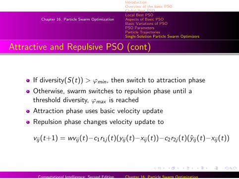
Attractive and Repulsive PSO (cont)
If diversity(S(t)) > ϕmin, then switch to attraction phase
Otherwise, swarm switches to repulsion phase until athreshold diversity, ϕmax is reached
Attraction phase uses basic velocity update
Repulsion phase changes velocity update to
vij(t+1) = wvij(t)−c1r1j(t)(yij(t)−xij(t))−c2r2j(t)(yij(t)−xij(t))
Computational Intelligence: Second Edition Chapter 16: Particle Swarm Optimization
Chapter 16. Particle Swarm Optimization
IntroductionOverview of the basic PSOGlobal Best PSOLocal Best PSOAspects of Basic PSOBasic Variations of PSOPSO ParametersParticle TrajectoriesSingle-Solution Particle Swarm Optimizers
Multi-Start PSO
Major problems with the basic PSO is lack of diversity whenparticles start to converge to the same point
Multi-start methods have as their main objective to increasediversity, whereby larger parts of the search space are explored
This is done by continually inject randomness, or chaos, intothe swarm
Note that continual injection of random positions will causethe swarm never to reach an equilibrium state
Methods should reduce chaos over time to ensure convergence
Computational Intelligence: Second Edition Chapter 16: Particle Swarm Optimization
Chapter 16. Particle Swarm Optimization
IntroductionOverview of the basic PSOGlobal Best PSOLocal Best PSOAspects of Basic PSOBasic Variations of PSOPSO ParametersParticle TrajectoriesSingle-Solution Particle Swarm Optimizers
Craziness PSO
Craziness is the process of randomly initializing some particles[7]
What are the issues in reinitialization?
What should be randomized?When should randomization occur?How should it be done?Which members of the swarm will be affected?What should be done with personal best positions of affectedparticles?
Computational Intelligence: Second Edition Chapter 16: Particle Swarm Optimization
Chapter 16. Particle Swarm Optimization
IntroductionOverview of the basic PSOGlobal Best PSOLocal Best PSOAspects of Basic PSOBasic Variations of PSOPSO ParametersParticle TrajectoriesSingle-Solution Particle Swarm Optimizers
Repelling Methods
The focus of repelling methods is to improve explorationabilities
Charged PSO:
Changes the velocity equation by adding a particleacceleration, ai :
vij(t + 1) = wvij(t) + c1r1(t)[yij(t)− xij(t)]
+ c2r2(t)[yj(t)− xij(t)]
+ aij(t)
Computational Intelligence: Second Edition Chapter 16: Particle Swarm Optimization
Chapter 16. Particle Swarm Optimization
IntroductionOverview of the basic PSOGlobal Best PSOLocal Best PSOAspects of Basic PSOBasic Variations of PSOPSO ParametersParticle TrajectoriesSingle-Solution Particle Swarm Optimizers
Charged PSO (cont)
The acceleration determines the magnitude of inter-particlerepulsion:
ai (t) =ns∑
l=1,i 6=l
ail(t)
The repulsion force between particles i and l defined as
ail(t) =
(
QiQl ((xi (t)−xl (t))||xi (t)−xl (t)||3
)if Rc ≤ ||xi (t)− xl(t)|| ≤ Rp(
QiQl (xi (t)−xl (t))R2
c ||xi (t)−xl (t)||
)if ||xi (t)− xl(t)|| < Rc
0 if ||xi (t)− xl(t)|| > Rp
where Qi is the charged magnitude of particle i
Computational Intelligence: Second Edition Chapter 16: Particle Swarm Optimization
Chapter 16. Particle Swarm Optimization
IntroductionOverview of the basic PSOGlobal Best PSOLocal Best PSOAspects of Basic PSOBasic Variations of PSOPSO ParametersParticle TrajectoriesSingle-Solution Particle Swarm Optimizers
Charged PSO (cont)
Neutral particles have a zero charged magnitude, i.e. Qi = 0
Inter-particle repulsion occurs only when the separationbetween two particles is within the range [Rc ,Rp]
Rc is the core radiusRp is the perception limit
The smaller the separation, the larger the repulsion betweenthe corresponding particles
The acceleration, ai (t), is determined for each particle beforethe velocity update
Computational Intelligence: Second Edition Chapter 16: Particle Swarm Optimization

Chapter 16. Particle Swarm Optimization
IntroductionOverview of the basic PSOGlobal Best PSOLocal Best PSOAspects of Basic PSOBasic Variations of PSOPSO ParametersParticle TrajectoriesSingle-Solution Particle Swarm Optimizers
Binary PSO
PSO was originally developed for continuous-valued searchspaces
Binary PSO was developed for binary-valued domains
Particles represent positions in binary space
xi ∈ Bnx , xij ∈ {0, 1}
Changes in a particle’s position then basically implies amutation of bits, by flipping a bit from one value to the other
Computational Intelligence: Second Edition Chapter 16: Particle Swarm Optimization
Chapter 16. Particle Swarm Optimization
IntroductionOverview of the basic PSOGlobal Best PSOLocal Best PSOAspects of Basic PSOBasic Variations of PSOPSO ParametersParticle TrajectoriesSingle-Solution Particle Swarm Optimizers
Binary PSO
Interpretation of velocity vector:
Velocity may be described by the number of bits that changeper iteration, which is the Hamming distance between xi (t)and xi (t + 1), denoted by H(xi (t), xi (t + 1))If H(xi (t), xi (t + 1)) = 0, zero bits are flipped and the particledoes not move; ||vi (t)|| = 0||vi (t)|| = nx is the maximum velocity, meaning that all bitsare flipped
Computational Intelligence: Second Edition Chapter 16: Particle Swarm Optimization
Chapter 16. Particle Swarm Optimization
IntroductionOverview of the basic PSOGlobal Best PSOLocal Best PSOAspects of Basic PSOBasic Variations of PSOPSO ParametersParticle TrajectoriesSingle-Solution Particle Swarm Optimizers
Binary PSO
Interpretation of velocity for a single dimension:
Velocity is used to calculate a probability of a bit flip:
v′
ij(t) = sig(vij(t)) =1
1 + e−vij (t)
Position update changes to
xij(t + 1) =
{1 if r3j(t) < sig(vij(t + 1))0 otherwise
Computational Intelligence: Second Edition Chapter 16: Particle Swarm Optimization
A.M. Abdelbar and S. Abdelshahid.Swarm Optimization with Instinct-Driven Particles.In Proceedings of the IEEE Congress on EvolutionaryComputation, pages 777–782, 2003.
M. Clerc and J. Kennedy.The Particle Swarm-Explosion, Stability, and Convergence in aMultidimensional Complex Space.IEEE Transactions on Evolutionary Computation, 6(1):58–73,2002.
R.C. Eberhart and J. Kennedy.A New Optimizer using Particle Swarm Theory.In Proceedings of the Sixth International Symposium onMicromachine and Human Science, pages 39–43, 1995.
102
Chapter 16. Particle Swarm Optimization
IntroductionOverview of the basic PSOGlobal Best PSOLocal Best PSOAspects of Basic PSOBasic Variations of PSOPSO ParametersParticle TrajectoriesSingle-Solution Particle Swarm Optimizers
H-Y. Fan.A Modification to Particle Swarm Optimization Algorithm.Engineering Computations, 19(7-8):970–989, 2002.
F. Heppner and U. Grenander.A Stochastic Nonlinear Model for Coordinated Bird Flocks.In S. Krasner, editor, The Ubiquity of Chaos. AAASPublications, 1990.
H. Higashi and H. Iba.Particle Swarm Optimization with Gaussian Mutation.In Proceedings of the IEEE Swarm Intelligence Symposium,pages 72–79, 2003.
J. Kennedy and R.C. Eberhart.
Computational Intelligence: Second Edition Chapter 16: Particle Swarm Optimization
Chapter 16. Particle Swarm Optimization
IntroductionOverview of the basic PSOGlobal Best PSOLocal Best PSOAspects of Basic PSOBasic Variations of PSOPSO ParametersParticle TrajectoriesSingle-Solution Particle Swarm Optimizers
Particle Swarm Optimization.In Proceedings of the IEEE International Joint Conference onNeural Networks, pages 1942–1948, 1995.
J. Kennedy and R. Mendes.Neighborhood Topologies in Fully-Informed andBest-of-Neighborhood Particle Swarms.In Proceedings of the IEEE International Workshop on SoftComputing in Industrial Applications, pages 45–50, 2003.
T. Krink and M. Løvberg.The Life Cycle Model: Combining Particle SwarmOptimisation, Genetic Algorithms and Hill Climbers.
Computational Intelligence: Second Edition Chapter 16: Particle Swarm Optimization
Chapter 16. Particle Swarm Optimization
IntroductionOverview of the basic PSOGlobal Best PSOLocal Best PSOAspects of Basic PSOBasic Variations of PSOPSO ParametersParticle TrajectoriesSingle-Solution Particle Swarm Optimizers
In Proceedings of the Parallel Problem Solving from NatureConference, Lecture Notes in Computer Science, volume 2439,pages 621–630. Springer-Verlag, 2002.
M. Løvberg.Improving Particle Swarm Optimization by Hybridization ofStochastic Search Heuristics and Self-Organized Criticality.Master’s thesis, Department of Computer Science, Universityof Aarhus, Denmark, 2002.
M. Løvberg, T.K. Rasmussen, and T. Krink.Hybrid Particle Swarm Optimiser with Breeding andSubpopulations.In Proceedings of the Genetic and Evolutionary ComputationConference, pages 469–476, 2001.
Computational Intelligence: Second Edition Chapter 16: Particle Swarm Optimization
Chapter 16. Particle Swarm Optimization
IntroductionOverview of the basic PSOGlobal Best PSOLocal Best PSOAspects of Basic PSOBasic Variations of PSOPSO ParametersParticle TrajectoriesSingle-Solution Particle Swarm Optimizers
C.W. Reynolds.Flocks, Herds, and Schools: A Distributed Behavioral Model.Computer Graphics, 21(4):25–34, 1987.
J.F. Schutte and A.A. Groenwold.Sizing Design of Truss Structures using Particle Swarms.Structural and Multidisciplinary Optimization, 25(4):261–269,2003.
B.R. Secrest and G.B. Lamont.Visualizing Particle Swarm Optimization – Gaussian ParticleSwarm Optimization.In Proceedings of the IEEE Swarm Intelligence Symposium,pages 198–204, 2003.
Computational Intelligence: Second Edition Chapter 16: Particle Swarm Optimization

Chapter 16. Particle Swarm Optimization
IntroductionOverview of the basic PSOGlobal Best PSOLocal Best PSOAspects of Basic PSOBasic Variations of PSOPSO ParametersParticle TrajectoriesSingle-Solution Particle Swarm Optimizers
Y. Shi and R.C. Eberhart.A Modified Particle Swarm Optimizer.In Proceedings of the IEEE Congress on EvolutionaryComputation, pages 69–73, 1998.
A. Silva, A. Neves, and E. Costa.An Empirical Comparison of Particle Swarm and Predator PreyOptimisation.In Proceedings of the Thirteenth Irish Conference on ArtificialIntelligence and Cognitive Science, Lecture Notes in ArtificialIntelligence, volume 2464, pages 103–110. Springer-Verlag,2002.
P.N. Suganthan.Particle Swarm Optimiser with Neighborhood Operator.
Computational Intelligence: Second Edition Chapter 16: Particle Swarm Optimization

Chapter 16. Particle Swarm Optimization
IntroductionOverview of the basic PSOGlobal Best PSOLocal Best PSOAspects of Basic PSOBasic Variations of PSOPSO ParametersParticle TrajectoriesSingle-Solution Particle Swarm Optimizers
In Proceedings of the IEEE Congress on EvolutionaryComputation, pages 1958–1962, 1999.
I.C. Trelea.The Particle Swarm Optimization Algorithm: ConvergenceAnalysis and Parameter Selection.Information Processing Letters, 85(6):317–325, 2003.
F. van den Bergh.An Analysis of Particle Swarm Optimizers.PhD thesis, Department of Computer Science, University ofPretoria, Pretoria, South Africa, 2002.
F. van den Bergh and A.P. Engelbrecht.Cooperative Learning in Neural Networks using Particle SwarmOptimizers.
Computational Intelligence: Second Edition Chapter 16: Particle Swarm Optimization
Chapter 16. Particle Swarm Optimization
IntroductionOverview of the basic PSOGlobal Best PSOLocal Best PSOAspects of Basic PSOBasic Variations of PSOPSO ParametersParticle TrajectoriesSingle-Solution Particle Swarm Optimizers
South African Computer Journal, 26:84–90, 2000.
F. van den Bergh and A.P. Engelbrecht.A Cooperative Approach to Particle Swarm Optimization.IEEE Transactions on Evolutionary Computation,8(3):225–239, 2004.
F. van den Bergh and A.P. Engelbrecht.A Study of Particle Swarm Optimization Particle Trajectories.Information Sciences, 176(8):937–971, 2006.
G. Venter and J. Sobieszczanski-Sobieski.Multidisciplinary Optimization of a Transport Aircraft Wingusing Particle Swarm Optimization.Structural and Multidisciplinary Optimization,26(1-2):121–131, 2003.
Computational Intelligence: Second Edition Chapter 16: Particle Swarm Optimization
Chapter 16. Particle Swarm Optimization
IntroductionOverview of the basic PSOGlobal Best PSOLocal Best PSOAspects of Basic PSOBasic Variations of PSOPSO ParametersParticle TrajectoriesSingle-Solution Particle Swarm Optimizers
W-J. Zhang and X-F. Xie.DEPSO: Hybrid Particle Swarm with Differential EvolutionOperator.In Proceedings of the IEEE International Conference onSystem, Man, and Cybernetics, volume 4, pages 3816–3821,2003.
Computational Intelligence: Second Edition Chapter 16: Particle Swarm Optimization