Embed Size (px)
Citation preview
415
15Indicating Forest Ecosystem and Stand Productivity: From Deductive to Inductive Concepts
Hans Pretzsch and Thomas Rötzer
CONTENTS
15.1 Introduction ........................................................................................................................ 41615.2 Relevance of Productivity to Ecological Forest Management ..................................... 416
15.2.1 Definitions and Base Processes of Forest Stand Productivity ......................... 41615.2.2 Relationship between Productivity and Forest Functions and Services ....... 419
15.3 Forest Ecosystem and Stand Productivity Worldwide .................................................42015.3.1 Global Values ..........................................................................................................42015.3.2 Productivity of Forest Ecological Zones .............................................................420
15.4 Indicators for Forest Ecosystem and Stand Productivity ............................................. 42415.4.1 Overall View of Indices for Estimating Site Productivity ................................ 42415.4.2 From Proxy Variables to “Primary” Factors for Explanations and
Estimations of Stand and Tree Growth ..............................................................42615.5 Effect of Forest Management on Forest Ecosystem and Stand Productivity ............428
15.5.1 Continuous versus Cyclic Stand Productivity ...................................................42815.5.2 Species Mixing Can Modify Productivity .........................................................42815.5.3 Relationship between Stand Density and Growth in Dependence on
Forest Structuring ..................................................................................................42915.6 Productivity Changes and Change Detection: Impact of Disturbance Events
and Long-Term Trends on Stand Productivity .............................................................. 43215.6.1 Long-Term Changes in Productivity ................................................................... 43215.6.2 Long-Term Plots as Ultimate Arbiters .................................................................43315.6.3 Current Growth Trends ........................................................................................435
15.7 Integration of Indicator Systems into Forest Management ..........................................43615.7.1 Productivity Regulation as a Basis for Many Other Forest Functions and
Services ....................................................................................................................43615.7.2 Stand Productivity and Sustainable Productivity at the Enterprise Level ..... 43615.7.3 Productivity Regulation in Forest Practices ....................................................... 437
15.8 Perspectives: From Deductive to Inductive and Static to Dynamic Indications of Forest Ecosystem and Stand Productivity .................................................................438
References ..................................................................................................................................... 439
© 2016 Taylor & Francis Group, LLC
416 Ecological Forest Management Handbook
15.1 Introduction
The productivity of forest ecosystems and stands represents their capacity of dry mat-ter synthesis and depends highly on external environmental conditions. Dry matter productivity is essential for ecological forest management as it determines most for-est functions and services. Carbon sequestration, abundance of decomposers, financial income of forest owners, and most other forest functions and services increase with for-est ecosystem and stand productivity. So information on productivity in the narrower sense was pivot for the dominant wood use paradigm but became even more important for ecological forest management because of its strong effect on all achievements in the modern forest basket.
For the purpose of clarity, the chapter starts with definitions of different aspects of pro-ductivity, which are applied for characterizing the world’s forests. Empirical knowledge on productivity comes mostly from long-term plots. However, forest practice cannot start long-term monitoring when information on productivity is required, but needs easy-to-measure indicators. We introduce such indicators for the production that can be realized at a certain site with a given species or genotype. We further show how this potential pro-ductivity can be modified by specified management regimes.
Historic litter raking, acid rain pollutant, and climate change are just a few out of many disturbances that massively modify productivity. We stress long-term survey for quanti-fying such human footprints on forest and for updating the level of productivity of forest ecosystems and stands even in a rapidly changing environment. Beyond their application for monitoring and controlling, indicators of productivity play a crucial role in strate-gic planning and decision making. Finally, it will be emphasized that earlier approaches deduced information about productivity from general models (e.g., yield tables, stand simulators), which were parameterized just by a small number of long-term experimental plots. Present-day inventories with repeated survey provide information on forest struc-ture, growth, yield, and site conditions, which enable site-specific induction of productiv-ity and replacement of the former inductive approaches.
Wood production and harvest were the exclusive purpose of productivity assessment in the past. This chapter will show that the productivity of forest ecosystems and stands determines nearly all sectors of ecological forest management covered in this hand-book, reaching from forest inventory, to planning and decision making, to monitor-ing, certification, conservation, regeneration, and even reclamation of devastated forest ecosystems.
15.2 Relevance of Productivity to Ecological Forest Management
15.2.1 Definitions and Base Processes of Forest Stand Productivity
Productivity of plants in an ecological sense means the fixation of solar energy and is referred to as gross primary productivity (GPP). In other words, GPP denotes the amount of carbon gained through photosynthesis for a given area over a given time. In forestry and ecology, GPP is often calculated as biomass production per hectare and year (Pretzsch 2009; Matyssek et al. 2010).
© 2016 Taylor & Francis Group, LLC
Dow
nloa
ded
by [
Tho
mas
Röt
zer]
at 0
3:18
18
Janu
ary
2016
417Indicating Forest Ecosystem and Stand Productivity
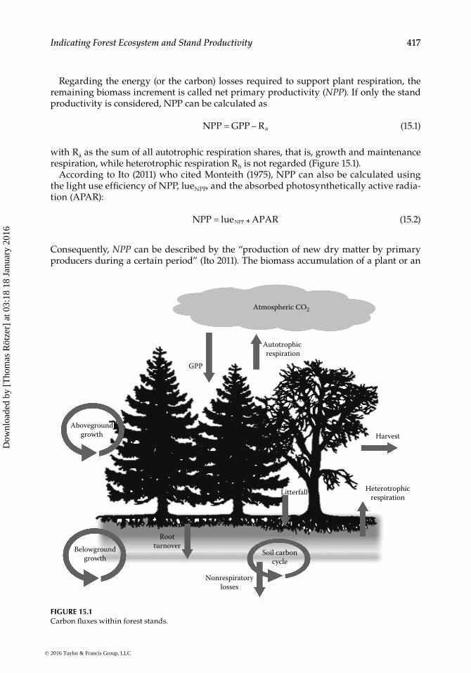
Regarding the energy (or the carbon) losses required to support plant respiration, the remaining biomass increment is called net primary productivity (NPP). If only the stand productivity is considered, NPP can be calculated as
NPP GPP Ra= – (15.1)
with Ra as the sum of all autotrophic respiration shares, that is, growth and maintenance respiration, while heterotrophic respiration Rh is not regarded (Figure 15.1).
According to Ito (2011) who cited Monteith (1975), NPP can also be calculated using the light use efficiency of NPP, lueNPP, and the absorbed photosynthetically active radia-tion (APAR):
NPP lue APARNPP= * (15.2)
Consequently, NPP can be described by the “production of new dry matter by primary producers during a certain period” (Ito 2011). The biomass accumulation of a plant or an
Atmospheric CO2
Heterotrophicrespiration
Harvest
Nonrespiratorylosses
Soil carboncycle
RootturnoverBelowground
growth
GPP
Autotrophic respiration
Abovegroundgrowth
Litterfall
FIGURE 15.1Carbon fluxes within forest stands.
© 2016 Taylor & Francis Group, LLC
Dow
nloa
ded
by [
Tho
mas
Röt
zer]
at 0
3:18
18
Janu
ary
2016
418 Ecological Forest Management Handbook
entire stand includes losses through plant organ turnover that is litterfall and branch, twig and root turnover, and losses through the mortality of the entire plants:
BA NPP losses mortality= - - (15.3)
BA is often called the net growth, which implies that the gross growth is equal to NPP (Pretzsch 2009).
Following Luyssaert et al. (2007), the net primary productivity for the individual com-partments of a tree or a stand can be split up in
NPP NPP NPP NPP NPPfoliage wood root reproduction= + + + (15.4)
where the net primary productivity of foliage, wood (stem and branches), roots (fine as well as coarse roots), and reproduction (flowers, seeds, fruits) is summed up.
According to Ito (2011) and Luyssaert et al. (2007), the NPP estimation can be extended for consumers:
NPP BA C C + l + l Cha he em ex my+ = + + + (15.5)
whereNPP+ is the modified net primary productivityCha and Che are the consumption by human harvest and herbivores, respectivelylem, lex denote losses by emissions such as biogenic volatile organic compounds (BVOCs)
or CH4 and losses by exudation of rootsCmy is the consumption by mycorrhiza
The described equations that can be used at different scales, such as GPP, NPP, and so on. Can be calculated for a single tree not only for an entire forest stand but also for one spe-cies of a given area. In addition, they can be scaled up for an entire ecosystem by including the heterotrophic respiration (Smith and Smith 2009) (Figure 15.1):
NEP GPP R Ra h= – – (15.6)
where NEP is the net ecosystem productivity.Further, if the import from surrounding ecosystems (imse) and nonrespiratory losses
(lnr) such as losses by forest fires, harvest, herbivores, or erosion is known (Buchmann and Schulze 1999; Chapin et al. 2006), the net biome productivity (NBP) can be calculated by
NBP NEP l imnr se= +– (15.7)
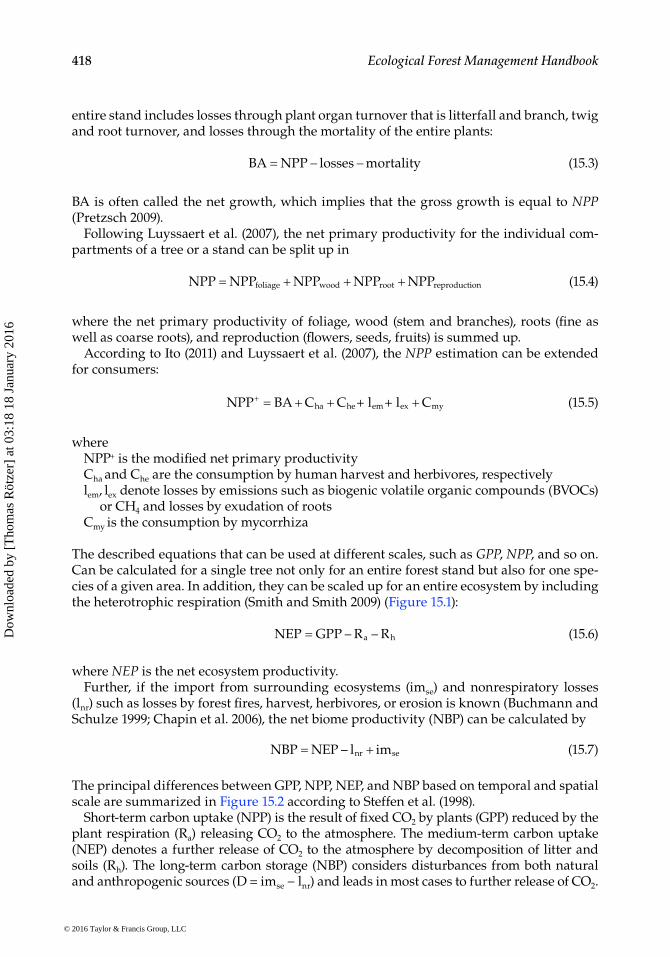
The principal differences between GPP, NPP, NEP, and NBP based on temporal and spatial scale are summarized in Figure 15.2 according to Steffen et al. (1998).
Short-term carbon uptake (NPP) is the result of fixed CO2 by plants (GPP) reduced by the plant respiration (Ra) releasing CO2 to the atmosphere. The medium-term carbon uptake (NEP) denotes a further release of CO2 to the atmosphere by decomposition of litter and soils (Rh). The long-term carbon storage (NBP) considers disturbances from both natural and anthropogenic sources (D = imse − lnr) and leads in most cases to further release of CO2.
© 2016 Taylor & Francis Group, LLC
Dow
nloa
ded
by [
Tho
mas
Röt
zer]
at 0
3:18
18
Janu
ary
2016
419Indicating Forest Ecosystem and Stand Productivity
Consequently, the temporal scale of plant productivity is closely linked with the spatial scale (individual tree, stand, ecosystem) regardless of the climate zone. This is also crucial when analyzing forest functions and services.
15.2.2 Relationship between Productivity and Forest Functions and Services
Information on productivity in the narrower sense was pivot for the dominant wood use paradigm (Yaffee 1999), but became even more important for ecological forest management because of its strong effect on all achievements in the contemporary basket of forest functions and services. The effect of productivity on other forest func-tions and services than wood production can differ a lot. Carbon sequestration and fossil fuel substitution can increase with productivity (Marland and Schlamadinger 1997), but groundwater supply often decreases (Dudley and Stolton 2003; Molden et al. 2003). The abundance of organisms rises (Vile et al. 2006), but the species rich-ness subsides with increasing forest productivity (Waide et al. 1999). While high pro-ductivities mean favorable financial income for the forest owner, it may reduce the aesthetic value and recreation function due to high stocking densities and missing views on the landscape.
Beyond the level of productivity, most forest functions and services are highly deter-mined by the management intensity in terms of wood harvest and removal. Positive effect of high productivity can turn into negative effects by nutrient export, which can be extremely high especially on high-productivity sites with high stocking and removal vol-ume and biomass. A lowering of the stand productivity by stand density reduction in the course of thinning may lower the drought stress of the trees, reduce the water consump-tion of the forest, and improve the recreation and aesthetic value by creating open space lookout points for forest walkers.
Positive effects of low productivity can be spoiled when low-productivity sites with high species richness are fertilized, drained, or transformed into plantations. Negative effects of low productivity, on the other hand, can be remedied by the establishment of species mixtures, among others, with atmospheric nitrogen–fixing species that may improve soil conditions and fertility.
As these examples illustrate, there is a trade-off between many productivity-determined forest functions and services already at the stand level and in a defined period. Including other spatial and temporal scales can further complicate the relationships and trade-offs.
AtmosphericCO2
GPP
Rh D
NBPNEPNPP
Longterm
Mediumterm
Shortterm
Ra
FIGURE 15.2Temporal and spatial scaling of plant productivity. (Adapted from Steffen, W. et al., Science, 280, 1393, 1998.)
© 2016 Taylor & Francis Group, LLC
Dow
nloa
ded
by [
Tho
mas
Röt
zer]
at 0
3:18
18
Janu
ary
2016
420 Ecological Forest Management Handbook
High-productivity plantations exclusively for wood supply may appear negative in terms of biodiversity seen at the stand level. However, if they help to establish conservation areas elsewhere, the assessment may change. How the various forest functions and services depending on and including productivity are weighted and realized ultimately depends on the legal frame and the objective of the forest owner.
15.3 Forest Ecosystem and Stand Productivity Worldwide
15.3.1 Global Values
Global terrestrial gross primary production is reported to be at 133 ± 15 Gt C year−1 (Piao et al. 2013). Global terrestrial NPP, on the other hand, was estimated at a mean value of 56.2 ± 14.3 Gt C year−1 based on 251 estimates published in 178 studies between 1862 and 2011 (Ito 2011). Due to the estimation methods, NPP varies between 46.2 ± 22.3 Gt C year−1 using inventory aggregation and 61.2 ± 9.4 Gt C year−1 using dynamic global vegetation models (Ito 2011). Carvalhais et al. (2014) estimate that the global gross primary production is 126.7 Gt year−1 on average resulting in a net primary production of 54 Gt year−1.
Assuming a total land area of approximately 149 × 106 km² (Saugier et al. 2001 or www.spacenews.de), the area-based GPP is 8.93 ± 1.01 t C ha−1 year−1, while the global average of NPP is 3.77 ± 0.96 t C ha−1 year−1. Higher NPP values were given by Saugier et al. (2001) with 4.19 t C ha−1 year−1.
Based on model simulations, several studies (e.g., Sitch et al. 2003; Ito 2011; Piao et al. 2013) reveal an NPP increase from preindustrial time to present that in most cases ranges between 10% and 30%. Piao et al. (2013), for example, found that NPP rises on average by 16% within simulation scenarios and by 13% within the FACE experiments per 100 ppm increase of atmospheric CO2 concentration.
The carbon use efficiency (cue) can be defined as the ratio between NPP and GPP. Because about 50% of the photosynthesis is spent for plant respiration, cue is commonly assumed to be 0.5. However, global cue values vary to a great extent between 0.33 and 0.88 (Ito 2011). Depending on the forest type, DeLucia et al. (2007) found cue values ranging from 0.23 up to 0.83.
15.3.2 Productivity of Forest Ecological Zones
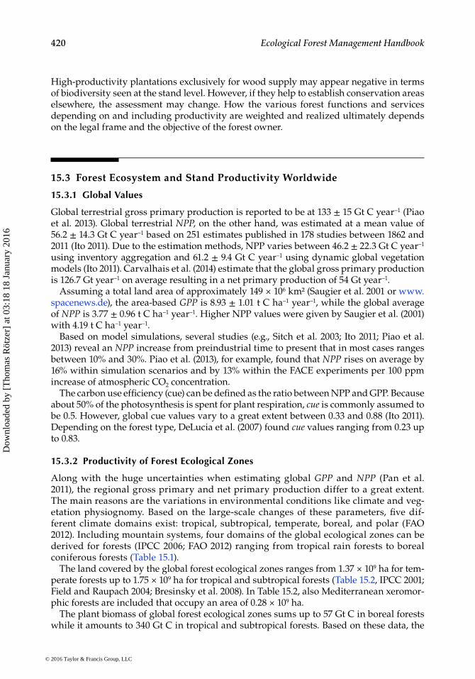
Along with the huge uncertainties when estimating global GPP and NPP (Pan et al. 2011), the regional gross primary and net primary production differ to a great extent. The main reasons are the variations in environmental conditions like climate and veg-etation physiognomy. Based on the large-scale changes of these parameters, five dif-ferent climate domains exist: tropical, subtropical, temperate, boreal, and polar (FAO 2012). Including mountain systems, four domains of the global ecological zones can be derived for forests (IPCC 2006; FAO 2012) ranging from tropical rain forests to boreal coniferous forests (Table 15.1).
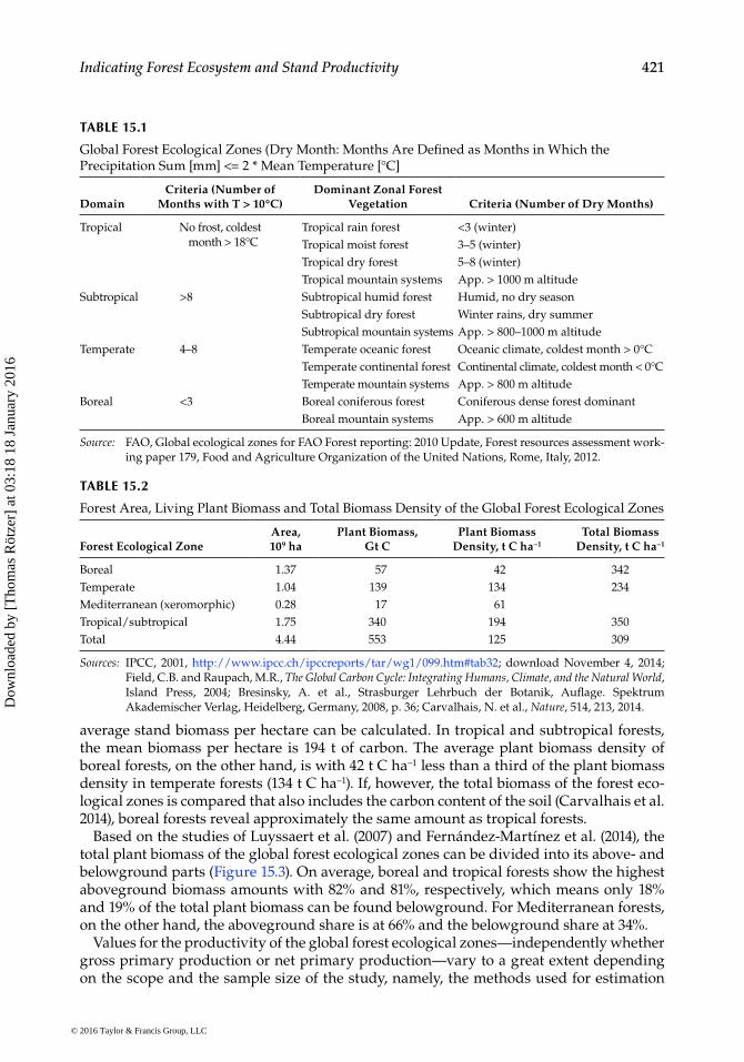
The land covered by the global forest ecological zones ranges from 1.37 × 10⁹ ha for tem-perate forests up to 1.75 × 10⁹ ha for tropical and subtropical forests (Table 15.2, IPCC 2001; Field and Raupach 2004; Bresinsky et al. 2008). In Table 15.2, also Mediterranean xeromor-phic forests are included that occupy an area of 0.28 × 10⁹ ha.
The plant biomass of global forest ecological zones sums up to 57 Gt C in boreal forests while it amounts to 340 Gt C in tropical and subtropical forests. Based on these data, the
© 2016 Taylor & Francis Group, LLC
Dow
nloa
ded
by [
Tho
mas
Röt
zer]
at 0
3:18
18
Janu
ary
2016
421Indicating Forest Ecosystem and Stand Productivity
average stand biomass per hectare can be calculated. In tropical and subtropical forests, the mean biomass per hectare is 194 t of carbon. The average plant biomass density of boreal forests, on the other hand, is with 42 t C ha−1 less than a third of the plant biomass density in temperate forests (134 t C ha−1). If, however, the total biomass of the forest eco-logical zones is compared that also includes the carbon content of the soil (Carvalhais et al. 2014), boreal forests reveal approximately the same amount as tropical forests.
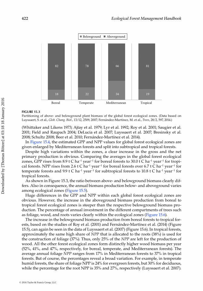
Based on the studies of Luyssaert et al. (2007) and Fernández-Martínez et al. (2014), the total plant biomass of the global forest ecological zones can be divided into its above- and belowground parts (Figure 15.3). On average, boreal and tropical forests show the highest aboveground biomass amounts with 82% and 81%, respectively, which means only 18% and 19% of the total plant biomass can be found belowground. For Mediterranean forests, on the other hand, the aboveground share is at 66% and the belowground share at 34%.
Values for the productivity of the global forest ecological zones—independently whether gross primary production or net primary production—vary to a great extent depending on the scope and the sample size of the study, namely, the methods used for estimation
TABLE 15.1
Global Forest Ecological Zones (Dry Month: Months Are Defined as Months in Which the Precipitation Sum [mm] <= 2 * Mean Temperature [°C]
Domain Criteria (Number of
Months with T > 10°C) Dominant Zonal Forest
Vegetation Criteria (Number of Dry Months)
Tropical No frost, coldest month > 18°C
Tropical rain forest <3 (winter)Tropical moist forest 3–5 (winter)Tropical dry forest 5–8 (winter)Tropical mountain systems App. > 1000 m altitude
Subtropical >8 Subtropical humid forest Humid, no dry seasonSubtropical dry forest Winter rains, dry summerSubtropical mountain systems App. > 800–1000 m altitude
Temperate 4–8 Temperate oceanic forest Oceanic climate, coldest month > 0°CTemperate continental forest Continental climate, coldest month < 0°CTemperate mountain systems App. > 800 m altitude
Boreal <3 Boreal coniferous forest Coniferous dense forest dominantBoreal mountain systems App. > 600 m altitude
Source: FAO, Global ecological zones for FAO Forest reporting: 2010 Update, Forest resources assessment work-ing paper 179, Food and Agriculture Organization of the United Nations, Rome, Italy, 2012.
TABLE 15.2
Forest Area, Living Plant Biomass and Total Biomass Density of the Global Forest Ecological Zones
Forest Ecological ZoneArea, 109 ha
Plant Biomass, Gt C
Plant Biomass Density, t C ha−1
Total Biomass Density, t C ha−1
Boreal 1.37 57 42 342Temperate 1.04 139 134 234Mediterranean (xeromorphic) 0.28 17 61Tropical/subtropical 1.75 340 194 350Total 4.44 553 125 309
Sources: IPCC, 2001, http://www.ipcc.ch/ipccreports/tar/wg1/099.htm#tab32; download November 4, 2014; Field, C.B. and Raupach, M.R., The Global Carbon Cycle: Integrating Humans, Climate, and the Natural World, Island Press, 2004; Bresinsky, A. et al., Strasburger Lehrbuch der Botanik, Auflage. Spektrum Akademischer Verlag, Heidelberg, Germany, 2008, p. 36; Carvalhais, N. et al., Nature, 514, 213, 2014.
© 2016 Taylor & Francis Group, LLC
Dow
nloa
ded
by [
Tho
mas
Röt
zer]
at 0
3:18
18
Janu
ary
2016
422 Ecological Forest Management Handbook
(Whittaker and Likens 1973; Ajtay et al. 1979; Lyr et al. 1992; Roy et al. 2001; Saugier et al. 2001; Field and Raupach 2004; DeLucia et al. 2007; Luyssaert et al. 2007; Bresinsky et al. 2008; Schultz 2008; Beer et al. 2010; Fernández-Martínez et al. 2014).
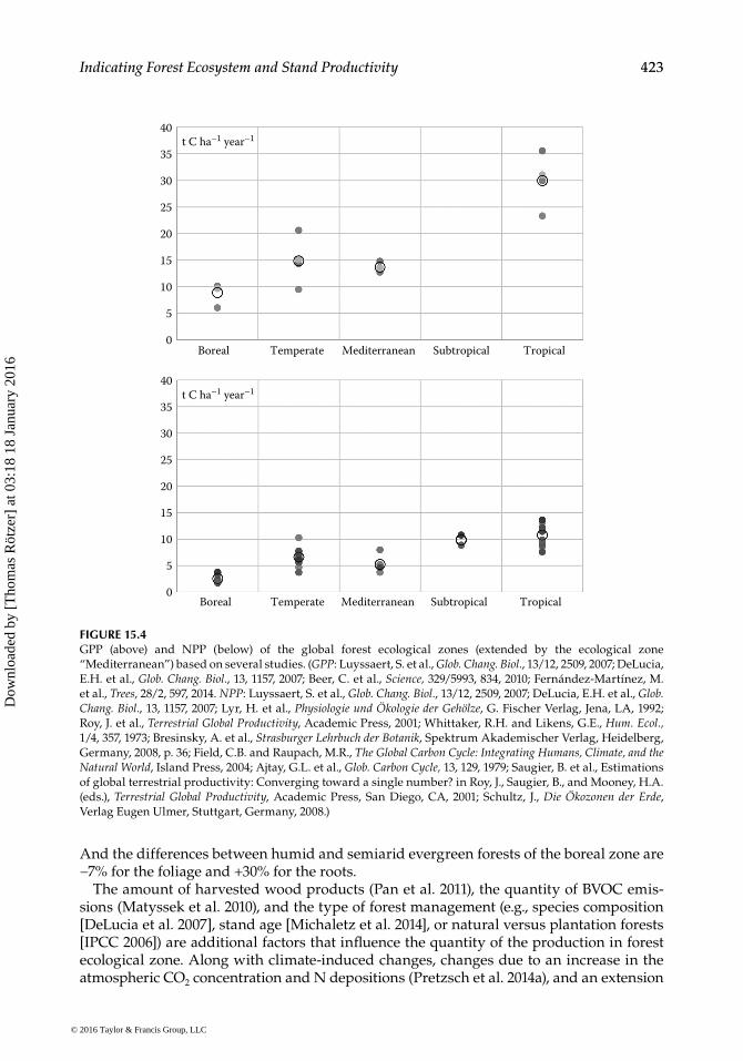
In Figure 15.4, the estimated GPP and NPP values for global forest ecological zones are given enlarged by Mediterranean forests and split into subtropical and tropical forests.
Despite high variations within the zones, a clear increase in the gross and the net primary production is obvious. Comparing the averages in the global forest ecological zones, GPP rises from 8.9 t C ha−1 year−1 for boreal forests to 30.0 t C ha−1 year−1 for tropi-cal forests. NPP rises from 2.6 t C ha−1 year−1 for boreal forests over 6.7 t C ha−1 year−1 for temperate forests and 9.9 t C ha−1 year−1 for subtropical forests to 10.8 t C ha−1 year−1 for tropical forests.
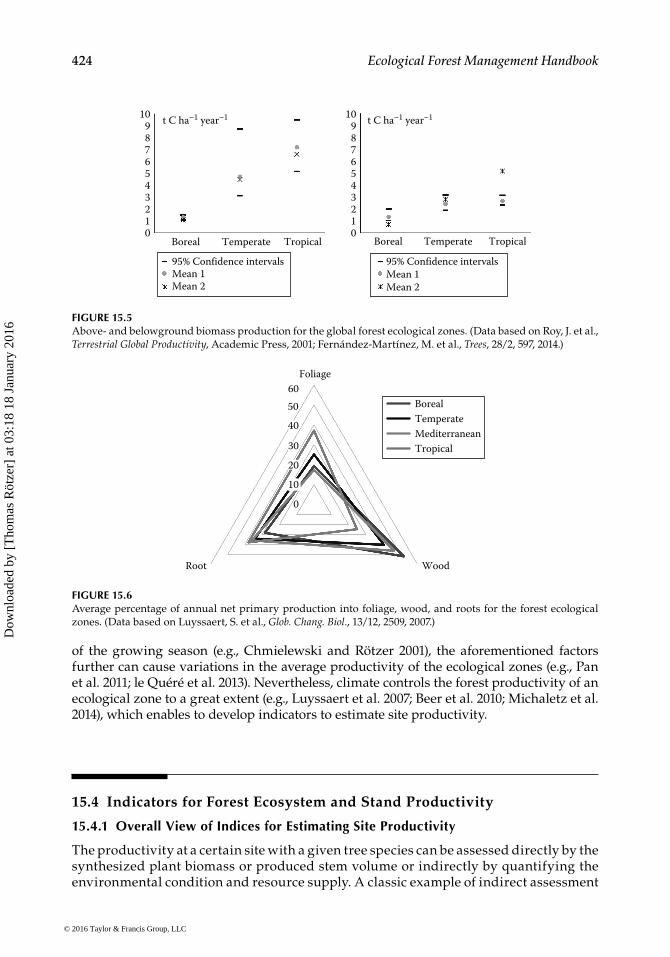
As shown in Figure 15.3, the ratio between above- and belowground biomass clearly dif-fers. Also in consequence, the annual biomass production below- and aboveground varies among ecological zones (Figure 15.5).
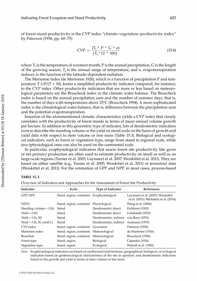
Huge differences in the GPP and NPP within each global forest ecological zones are obvious. However, the increase in the aboveground biomass production from boreal to tropical forest ecological zones is steeper than the respective belowground biomass pro-duction. The percentage of annual investment in the different compartments of trees such as foliage, wood, and roots varies clearly within the ecological zones (Figure 15.6).
The increase in the belowground biomass production from boreal forests to tropical for-ests, based on the studies of Roy et al. (2001) and Fernández-Martínez et al. (2014) (Figure 15.5), can again be seen in the data of Luyssaert et al. (2007) (Figure 15.6). In tropical forests, approximately the same high share of NPP that is allocated to the roots (38%) is used for the construction of foliage (37%). Thus, only 25% of the NPP are left for the production of wood. All the other forest ecological zones form distinctly higher wood biomass per year (52%, 41%, and 47%, respectively, for boreal, temperate, and Mediterranean forests). The average annual foliage NPP ranges from 17% in Mediterranean forests to 37% in tropical forests. But of course, the percentages reveal a broad variation. For example, in temperate humid forests, the share of foliage NPP is 24% for evergreen forests, but 30% for deciduous, while the percentage for the root NPP is 35% and 27%, respectively (Luyssaert et al. 2007).
Belowground Aboveground
82 78 66 81
18 22 34 19
Boreal Temperate TropicalMediterranean
FIGURE 15.3Partitioning of above- and belowground plant biomass of the global forest ecological zones. (Data based on Luyssaert, S. et al., Glob. Chang. Biol., 13/12, 2509, 2007; Fernández-Martínez, M. et al., Trees, 28/2, 597, 2014.)
© 2016 Taylor & Francis Group, LLC
Dow
nloa
ded
by [
Tho
mas
Röt
zer]
at 0
3:18
18
Janu
ary
2016
423Indicating Forest Ecosystem and Stand Productivity
And the differences between humid and semiarid evergreen forests of the boreal zone are −7% for the foliage and +30% for the roots.
The amount of harvested wood products (Pan et al. 2011), the quantity of BVOC emis-sions (Matyssek et al. 2010), and the type of forest management (e.g., species composition [DeLucia et al. 2007], stand age [Michaletz et al. 2014], or natural versus plantation forests [IPCC 2006]) are additional factors that influence the quantity of the production in forest ecological zone. Along with climate-induced changes, changes due to an increase in the atmospheric CO2 concentration and N depositions (Pretzsch et al. 2014a), and an extension
40
35
30
25
20
15
10
5
0
40
35
30
25
20
15
10
5
0
Boreal Temperate Mediterranean Subtropical
t C ha–1 year–1
t C ha–1 year–1
Tropical
Boreal Temperate Mediterranean Subtropical Tropical
FIGURE 15.4GPP (above) and NPP (below) of the global forest ecological zones (extended by the ecological zone “Mediterranean”) based on several studies. (GPP: Luyssaert, S. et al., Glob. Chang. Biol., 13/12, 2509, 2007; DeLucia, E.H. et al., Glob. Chang. Biol., 13, 1157, 2007; Beer, C. et al., Science, 329/5993, 834, 2010; Fernández-Martínez, M. et al., Trees, 28/2, 597, 2014. NPP: Luyssaert, S. et al., Glob. Chang. Biol., 13/12, 2509, 2007; DeLucia, E.H. et al., Glob. Chang. Biol., 13, 1157, 2007; Lyr, H. et al., Physiologie und Ökologie der Gehölze, G. Fischer Verlag, Jena, LA, 1992; Roy, J. et al., Terrestrial Global Productivity, Academic Press, 2001; Whittaker, R.H. and Likens, G.E., Hum. Ecol., 1/4, 357, 1973; Bresinsky, A. et al., Strasburger Lehrbuch der Botanik, Spektrum Akademischer Verlag, Heidelberg, Germany, 2008, p. 36; Field, C.B. and Raupach, M.R., The Global Carbon Cycle: Integrating Humans, Climate, and the Natural World, Island Press, 2004; Ajtay, G.L. et al., Glob. Carbon Cycle, 13, 129, 1979; Saugier, B. et al., Estimations of global terrestrial productivity: Converging toward a single number? in Roy, J., Saugier, B., and Mooney, H.A. (eds.), Terrestrial Global Productivity, Academic Press, San Diego, CA, 2001; Schultz, J., Die Ökozonen der Erde, Verlag Eugen Ulmer, Stuttgart, Germany, 2008.)
© 2016 Taylor & Francis Group, LLC
Dow
nloa
ded
by [
Tho
mas
Röt
zer]
at 0
3:18
18
Janu
ary
2016
424 Ecological Forest Management Handbook
of the growing season (e.g., Chmielewski and Rötzer 2001), the aforementioned factors further can cause variations in the average productivity of the ecological zones (e.g., Pan et al. 2011; le Quéré et al. 2013). Nevertheless, climate controls the forest productivity of an ecological zone to a great extent (e.g., Luyssaert et al. 2007; Beer et al. 2010; Michaletz et al. 2014), which enables to develop indicators to estimate site productivity.
15.4 Indicators for Forest Ecosystem and Stand Productivity
15.4.1 Overall View of Indices for Estimating Site Productivity
The productivity at a certain site with a given tree species can be assessed directly by the synthesized plant biomass or produced stem volume or indirectly by quantifying the environmental condition and resource supply. A classic example of indirect assessment
20
10
0
30
40
50
60Foliage
BorealTemperateMediterraneanTropical
Root Wood
FIGURE 15.6Average percentage of annual net primary production into foliage, wood, and roots for the forest ecological zones. (Data based on Luyssaert, S. et al., Glob. Chang. Biol., 13/12, 2509, 2007.)
109876543210
109876543210
Boreal Temperate
t C ha–1 year–1 t C ha–1 year–1
Tropical
95% Confidence intervalsMean 1Mean 2
Boreal Temperate Tropical
95% Confidence intervalsMean 1Mean 2
FIGURE 15.5Above- and belowground biomass production for the global forest ecological zones. (Data based on Roy, J. et al., Terrestrial Global Productivity, Academic Press, 2001; Fernández-Martínez, M. et al., Trees, 28/2, 597, 2014.)
© 2016 Taylor & Francis Group, LLC
Dow
nloa
ded
by [
Tho
mas
Röt
zer]
at 0
3:18
18
Janu
ary
2016
425Indicating Forest Ecosystem and Stand Productivity
of forest stand productivity is the CVP index “climate–vegetation– productivity index” by Paterson (1956, pp. 68–75)
CVP
T P G eT 12 1v
a=
( )( * * * )
* * 00 (15.8)
where Tv is the temperature of warmest month, P is the annual precipitation, G is the length of the growing season, Ta is the annual range of temperature, and e, evapotranspiration reducer, is the function of the latitude-dependent radiation.
The Martonne index (de Martonne 1926), which is a function of precipitation P and tem-perature T (=P/(T + 10), forms a simplified productivity indicator compared, for instance, to the CVP index. Other productivity indicators that are more or less based on meteoro-logical parameters are the Bruscheck index or the climatic water balance. The Bruscheck index is based on the annual precipitation sum and the number of summer days, that is, the number of days with temperatures above 25°C (Bruscheck 1994). A more sophisticated index is the climatological water balance, that is, difference between the precipitation sum and the potential evapotranspiration.
Insertion of the aforementioned climatic characteristics yields a CVP index that closely correlates with the productivity of forest stands in terms of mean annual volume growth per hectare. In addition to this geocentric type of indicator, lots of dendrometric indicators exist to describe the standing volume or the yield on stand scale on the basis of growth and yield data with respect to stem volume or tree mass (Table 15.3). Biological and ecologi-cal indicators, such as forest or vegetation type, range from stand to regional scale, while (eco-)physiological ones can also be used on the continental scale.
In particular, ecophysiological indicators that assess forest site productivity like gross or net primary production are often used to estimate productivity on small as well as on large-scale regions (Turner et al. 2005; Luyssaert et al. 2007; Weiskittel et al. 2011). They are based on either satellite (e.g., Turner et al. 2005; Weiskittel et al. 2011) or terrestrial data (Weiskittel et al. 2011). For the estimation of GPP and NPP, in most cases, process-based
TABLE 15.3
Overview of Indicators and Approaches for the Assessment of Forest Site Productivity
Indicator Scale Type of Indicator References
GPP, NPP Stand, region, continent Ecophysiological Luyssaert et al. (2007); Weiskittel et al. (2011); Michaletz et al. (2014)
NDVI Stand, region, continent Physiological Wang et al. (2004)Standing volume = f (h) Stand Dendrometric direct Eichhorn (1902)Yield = f (h) Stand Dendrometric direct Gehrhardt (1923)Yield = f (h, SI) Stand Dendrometric, indirect von Baur (1876)Yield = f (h, SI, yield l.) Stand Dendrometric, indirect Assmann (1970)CVP index Stand, region, continent Geocentric Paterson (1956)Martonne index Stand, region, continent Meteorological de Martonne (1926)Bruschek Stand, region, continent Meteorological Bruscheck (1994)Forest type Stand, region Biological Cajander (1926)Vegetation type Stand, region Ecological Wykoff et al. (1982)
Note: Ecophysiological indicators are based on synthesized total biomass; geographical, biological, or ecological indicators based on geobioecological characteristics of the site in question; and dendrometric indicators based on the growth and yield in terms of stem volume or tree mass.
© 2016 Taylor & Francis Group, LLC
Dow
nloa
ded
by [
Tho
mas
Röt
zer]
at 0
3:18
18
Janu
ary
2016
426 Ecological Forest Management Handbook
models form the base of the calculations. Weiskittel et al. (2011), for example, use the 3PG model, while Pretzsch et al. (2012) based their calculations on the model BALANCE, which is able to calculate productivity indicators also for structured forests like mixed stands (Rötzer et al. 2009). If the light use efficiency of a tree species is known, NPP can be derived from the APAR (Ito 2011). Eddy covariance measurements are another way to estimate ecophysiological indicators.
15.4.2 From Proxy Variables to “Primary” Factors for Explanations and Estimations of Stand and Tree Growth
The attempt to assess, classify, understand, and even estimate primary productivity, growth, or yield for a given forest stand from causal variables has been investigated in for-est research since the first experiments in the 18th century (Assmann 1970). However, the approaches have become more and more mechanistic and more focused on the primary resource and environmental variables. Initially, in the 18th century, the standing stem vol-ume of forest stands was used for the classification of a given stand into a site quality system (Pressler 1877):
Site fertility class f standing volume stand age= ( ), (15.9)
And then the site fertility class could be applied to estimate growth and yield, for example,
Volume growth f site class stand age= ( ), (15.10)
This classification was somehow circular; the standing volume must be estimated before determining the site fertility class, after which projections of the future volume productiv-ity could be calculated. This approach only made sense as long as light and moderate thin-nings were common. With the change to more intensive management concepts in the 19th century, the thinning component of total production increased so that standing volume became an increasingly poorer indicator of site fertility class.
As the relationship between stand age and stand height correlates closely with total stand production (Eichhorn 1902) and is less dependent on thinning intensity, it provides an alternative to the former approach. Thus, the use of age and mean height, introduced by von Baur (1876, 1881) and Perthuis de Laillevault (1803),
Site fertility class f mean height stand age= ( ), (15.11)
for the classification of stand growth became recognized despite some reluctance in the beginning (Heyer 1845). Estimates of stand growth and yield result from
Stand growth f site fertility class stand age= ( ), (15.12)
With the intensification of thinning from below, which significantly influences calcula-tions of mean height, another change was made in the mid-20th century toward the use of top height as an indicator of site fertility (Assmann 1970). The idea of using stand volume or height growth as a “phytometer” for the productivity of a site has continued to the present day. However, this approach is again being questioned as forest practice increas-ingly implements thinning from above in management regimes to encourage structurally
© 2016 Taylor & Francis Group, LLC
Dow
nloa
ded
by [
Tho
mas
Röt
zer]
at 0
3:18
18
Janu
ary
2016
427Indicating Forest Ecosystem and Stand Productivity
diverse mixed stands. The more a stand deviates from an even-aged, monolayered struc-ture, the greater the influence of density and competition on the relationships between age and height, and the less suitable the age–height relationship becomes an indicator of site fertility. Especially in highly structured mixed stands, mean and top heights are unsuit-able as site fertility indicators.
Heyer (1845) demanded that yield studies not be directed exclusively toward the vol-ume yield but toward the investigation and measurement of “primary site factors,” such as temperature, nutrient supply, and radiation. One step into this direction was made by Cajander (1926). He developed a classification system for boreal forests that facilitated the growth and yield estimation from the forest floor vegetation as the indicator (species lichens, mosses, grasses, herbs, shrubs). While this method became standard in the rather uniform and undisturbed boreal forests, the heterogeneity of forest types and human influences makes this approach inadequate for central European forests.
However, the core of Cajander’s idea was to combine locally available indicator variables for classifying a particular stand with growth and yield information deduced from site-specific yield tables. The increasing availability of site information and growth and yield data from inventories led to an increased meshing of locally acquired information about site, growth, and yield with general growth and yield relationships deduced from models. Moosmayer and Schöpfer (1972), Wykoff et al. (1982), and Wykoff and Monserud (1988) developed relationships between site conditions and growth at the tree or stand level by regression analysis:
Volume growth f stand attributes site characteristics= ( ), (15.13)
As independent variables, they used metric information (e.g., annual precipitation, mean temperature, slope, exposition) and nominal (e.g., levels of nutrition supply, levels of water supply) and ordinal (e.g., growth region, degree of disturbance of topsoil by machines) variables. To estimate the potential height growth, volume growth, and yield in the forest growth simulator SILVA, Kahn (1994) used a set of nine metric site variables.
Experimental field plots, monitoring plots, and chamber experiments enable the study of metabolic, physiologic, and growth process as well as the factors affecting growth (envi-ronmental conditions, resource supply) at increasingly more refined spatial and temporal resolution. For example, temperature measured per day, hour or minute, and radiation recorded separately for different wavelengths can be used to estimate the net primary production, according to the following approach:
NPP f leaf area radiation temperature nutrient water= ( ), , , , (15.14)
Simultaneously recorded assimilation rate, respiration, height, and diameter enable a refined estimation also of gross production (gC min−1, cm day−1, mm day−1) to be made. The development of inventory monitoring and innovative regionalization tools, which deliver all the relevant variables for such primary variable–based approaches Heyer (1845) already had in mind, is in progress. Knowledge about site–growth relationship forms the backbone of forest growth models, and hence, the availability of site variables is decisive for the applicability of these models. To overcome the lack of knowledge about the relationships between the primary causes affecting tree and stand develop-ment (environmental conditions, resource supply), forest research has gathered much rich experience in the application of “surrogate variables” or “proxy variables” (Oliver and
© 2016 Taylor & Francis Group, LLC
Dow
nloa
ded
by [
Tho
mas
Röt
zer]
at 0
3:18
18
Janu
ary
2016
428 Ecological Forest Management Handbook
Larson 1990; Zeide 2003). Examples for the application of a “surrogate variable” or “proxy variable” include the use of age–height relationships for estimations of stand growth, the area available for the growth or growing space of a tree for estimations of its resource supply, or the application of competition indices for estimations of height and diameter increment of an individual tree in relation to resource supply. In all cases, the primary factors remain unsolved. However, they are replaced by easy-to-measure auxiliary vari-ables although they merely reflect only the hidden relationships.
15.5 Effect of Forest Management on Forest Ecosystem and Stand Productivity
15.5.1 Continuous versus Cyclic Stand Productivity
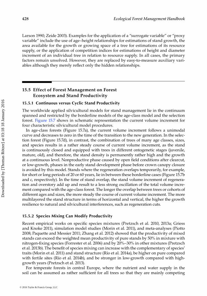
The worldwide applied silvicultural models for stand management lie in the continuum spanned and restricted by the borderline models of the age-class model and the selection forest. Figure 15.7 shows in schematic representation the current volume increment for four characteristic silvicultural model procedures.
In age-class forests (Figure 15.7a), the current volume increment follows a unimodal curve and decreases to zero in the time of the transition to the new generation. In the selec-tion forest (Figure 15.7d), in contrast, the combination of trees of many age classes, sizes, and species results in a rather steady course of current volume increment, as the stand is continuously closed and equipped with trees in different ontogenetic stages (juvenile, mature, old), and therefore, the stand density is permanently rather high and the growth at a continuous level. Nonproductive phase caused by open field conditions after clearcut, or low-growth, phases in the early stand development phase before crown canopy closure is avoided by this model. Stands where the regeneration overlaps temporarily, for example, for short or long periods of 20 or 60 years, lie in between these borderline cases (Figure 15.7b and c, respectively). In the time of stand overlap, the stand volume increment of regenera-tion and overstory add up and result to a less strong oscillation of the total volume incre-ment compared with the age-class forest. The longer the overlap between trees or cohorts of different ages and sizes, the more steady the course of current volume increment. The more multilayered the stand structure in terms of horizontal and vertical, the higher the growth resilience to natural and silvicultural interferences, such as regeneration cuts.
15.5.2 Species Mixing Can Modify Productivity
Recent empirical works on specific species mixtures (Pretzsch et al. 2010, 2013a; Griess and Knoke 2011), simulation model studies (Morin et al. 2011), and meta-analyses (Piotto 2008; Paquette and Messier 2011; Zhang et al. 2012) showed that the productivity of mixed stands can exceed the weighted mean productivity of pure stands by 50% in mixture with nitrogen-fixing species (Forrester et al. 2006) and by 20%–30% in other mixtures (Pretzsch et al. 2013b). The benefit of species mixing can increase with the complementary of species’ traits (Morin et al. 2011) and stand structure (Río et al. 2014a), be higher on pure compared with fertile sites (Río et al. 2014b), and be stronger in low-growth compared with high-growth years (Pretzsch et al. 2013).
For temperate forests in central Europe, where the nutrient and water supply in the soil can be assumed as rather sufficient for all trees so that they are mainly competing
© 2016 Taylor & Francis Group, LLC
Dow
nloa
ded
by [
Tho
mas
Röt
zer]
at 0
3:18
18
Janu
ary
2016
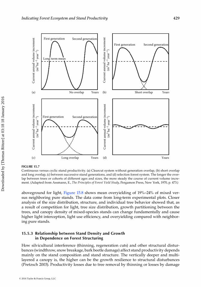
429Indicating Forest Ecosystem and Stand Productivity
aboveground for light, Figure 15.8 shows mean overyielding of 19%–24% of mixed ver-sus neighboring pure stands. The data come from long-term experimental plots. Closer analysis of the size distribution, structure, and individual tree behavior showed that, as a result of competition for light, tree size distribution, growth partitioning between the trees, and canopy density of mixed-species stands can change fundamentally and cause higher light interception, light use efficiency, and overyielding compared with neighbor-ing pure stands.
15.5.3 Relationship between Stand Density and Growth in Dependence on Forest Structuring
How silvicultural interference (thinning, regeneration cuts) and other structural distur-bances (windthrow, snow breakage, bark beetle damage) affect stand productivity depends mainly on the stand composition and stand structure. The vertically deeper and multi-layered a canopy is, the higher can be the growth resilience to structural disturbances (Pretzsch 2003). Productivity losses due to tree removal by thinning or losses by damage
Second generationFirst generation
Long overlap
Cur
rent
ann
ual v
olum
e in
crem
ent
(m3
ha–1
yea
r–1)
Cur
rent
ann
ual v
olum
e in
crem
ent
(m3 h
a–1 y
ear–1
)
(c) (d)Years Years
Cur
rent
ann
ual v
olum
e in
crem
ent
(m3
ha–1
yea
r–1)
Second generationFirst generation
Long-term mean
No overlap(a) Years
Second generationFirst generation
Short overlap
Cur
rent
ann
ual v
olum
e in
crem
ent
(m3 h
a–1 y
ear–1
)
(b) Years
FIGURE 15.7Continuous versus cyclic stand productivity. (a) Clearcut system without generation overlap, (b) short overlap and long overlap, (c) between successive stand generations, and (d) selection forest system. The longer the over-lap between trees or cohorts of different ages and sizes, the more steady the course of current volume incre-ment. (Adapted from Assmann, E., The Principles of Forest Yield Study, Pergamon Press, New York, 1970, p. 473.)
© 2016 Taylor & Francis Group, LLC
Dow
nloa
ded
by [
Tho
mas
Röt
zer]
at 0
3:18
18
Janu
ary
2016
430 Ecological Forest Management Handbook
Spruce–Beech
Relative Difference (95% Cl)
0.87 (0.71, 1.06)0.95 (0.85, 1.06)0.98 (0.93, 1.02)
0.99 (0.81, 1.21)
1.15 (1.03, 1.28)
2.02 (1.51, 2.72)
1.19 (1.08, 1.31)
2.00 (1.68, 2.38)1.70 (1.50, 1.94)1.59 (1.30, 1.95)1.30 (0.98, 1.72)1.25 (1.00, 1.56)1.19 (1.13, 1.26)1.18 (1.03, 1.35)
1.14 (1.05, 1.24)1.14 (0.95, 1.36)1.13 (0.94, 1.37)1.11 (0.94, 1.31)1.07 (0.99, 1.16)1.05 (1.00, 1.11)
0.99 (0.91, 1.07)
Ehingen 51
Experimental Plot
WiedemannMitterteich 101Westerhof 131b37Westerhof 131b31Wieda 114Zwiesel 111Uslar 57Daun 1207Zwiesel 134Knobben 44 1/2NP 602Daun 1206Zwiesel 135Geislingen 76Morbach 1501Freising 813Nordhalben 811Murten 20Schongau 814
RE Model
0.61 1.00 1.65 2.72Mixed Stand/Pure Stand(a)
Relative Difference (95% Cl)Experimental Plot
Concise
Oak–Beech
Waldbrunn 106Gryfino 35DhroneckenGryfino 33Ebrach 132Waldbrunn 105Main-tauber 86Jossgrund 151Ebrach 133Hochstift 619SchluechtemHochstift 618BalmisHochstift 617EichbuehlRothenbuch 801
Rohrbrunn 314Kelheim 804
Re Model
0.73 (0.60, 0.89)0.84 (0.81, 0.87)0.86 (0.78, 0.94)0.95 (0.81, 1.11)0.96 (0.86, 1.07)0.97 (0.75, 1.25)1.00 (0.91, 1.11)1.04 (0.99, 1.10)1.12 (1.02, 1.22)1.23 (0.96, 1.58)1.24 (1.07, 1.43)
1.42 (1.32, 1.52)1.48 (1.35, 1.63)
2.24 (1.88, 2.67)2.43 (1.96, 3.01)2.53 (1.90, 3.37)
1.24 (1.06, 1.45)
0.37
1.80 (1.30, 2.49)
1.30 (1.19, 1.42)1.27 (0.95, 1.69)
0.61 1.00 1.65 2.72Mixed Stand/Pure Stand(b)
4.48
FIGURE 15.8Comparison of the stand productivity of mixed versus pure forest stands based on long-term experimental plots of (a) Norway spruce and European beech; (b) sessile oak and European beech. (Continued)
© 2016 Taylor & Francis Group, LLC
Dow
nloa
ded
by [
Tho
mas
Röt
zer]
at 0
3:18
18
Janu
ary
2016
431Indicating Forest Ecosystem and Stand Productivity
can be better compensated by the presence of a second or third layer of trees that might immediately use the resources not any longer intercepted by the removal of trees.
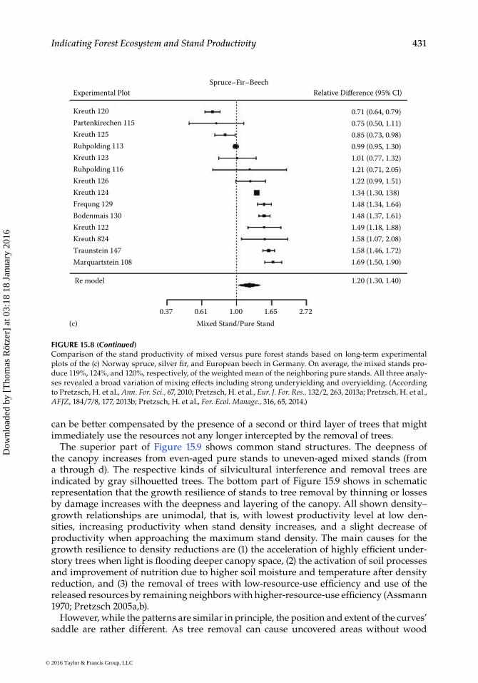
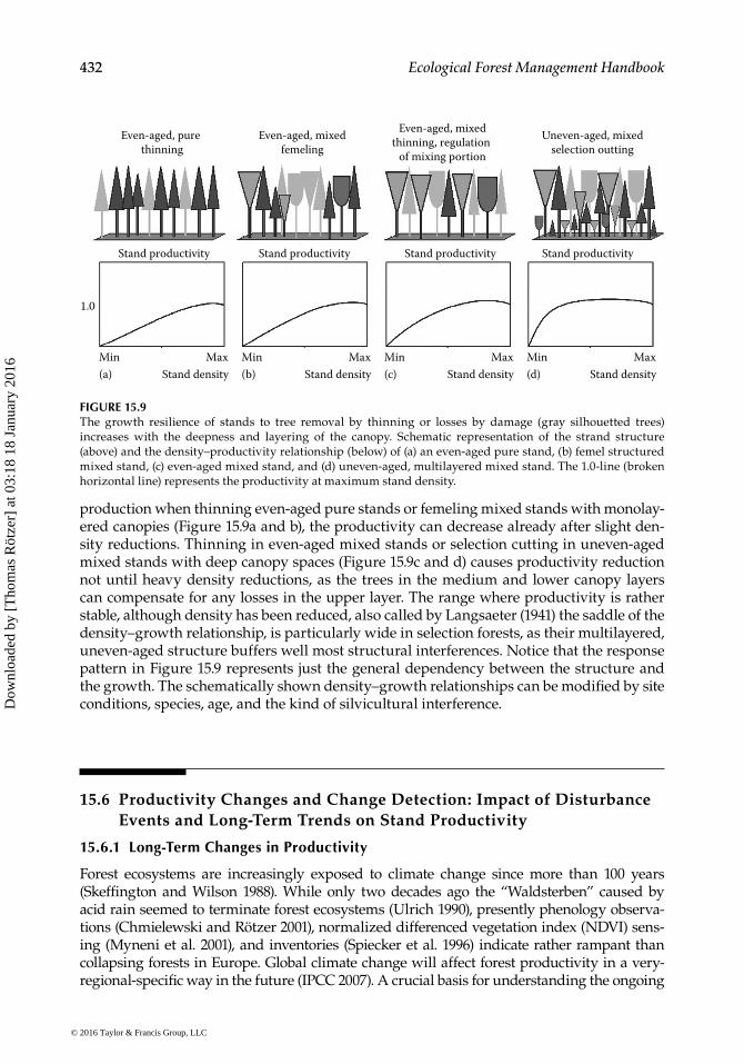
The superior part of Figure 15.9 shows common stand structures. The deepness of the canopy increases from even-aged pure stands to uneven-aged mixed stands (from a through d). The respective kinds of silvicultural interference and removal trees are indicated by gray silhouetted trees. The bottom part of Figure 15.9 shows in schematic representation that the growth resilience of stands to tree removal by thinning or losses by damage increases with the deepness and layering of the canopy. All shown density–growth relationships are unimodal, that is, with lowest productivity level at low den-sities, increasing productivity when stand density increases, and a slight decrease of productivity when approaching the maximum stand density. The main causes for the growth resilience to density reductions are (1) the acceleration of highly efficient under-story trees when light is flooding deeper canopy space, (2) the activation of soil processes and improvement of nutrition due to higher soil moisture and temperature after density reduction, and (3) the removal of trees with low-resource-use efficiency and use of the released resources by remaining neighbors with higher-resource-use efficiency (Assmann 1970; Pretzsch 2005a,b).
However, while the patterns are similar in principle, the position and extent of the curves’ saddle are rather different. As tree removal can cause uncovered areas without wood
Spruce–Fir–BeechExperimental Plot
Kreuth 120 0.71 (0.64, 0.79)
Relative Difference (95% Cl)
Partenkirechen 115Kreuth 125Ruhpolding 113Kreuth 123Ruhpolding 116Kreuth 126Kreuth 124Frequng 129Bodenmais 130Kreuth 122Kreuth 824Traunstein 147Marquartstein 108
Re model
0.37
0.75 (0.50, 1.11)0.85 (0.73, 0.98)0.99 (0.95, 1.30)1.01 (0.77, 1.32)1.21 (0.71, 2.05)1.22 (0.99, 1.51)1.34 (1.30, 138)1.48 (1.34, 1.64)1.48 (1.37, 1.61)1.49 (1.18, 1.88)1.58 (1.07, 2.08)1.58 (1.46, 1.72)1.69 (1.50, 1.90)
1.20 (1.30, 1.40)
0.61 1.00 1.65 2.72Mixed Stand/Pure Stand(c)
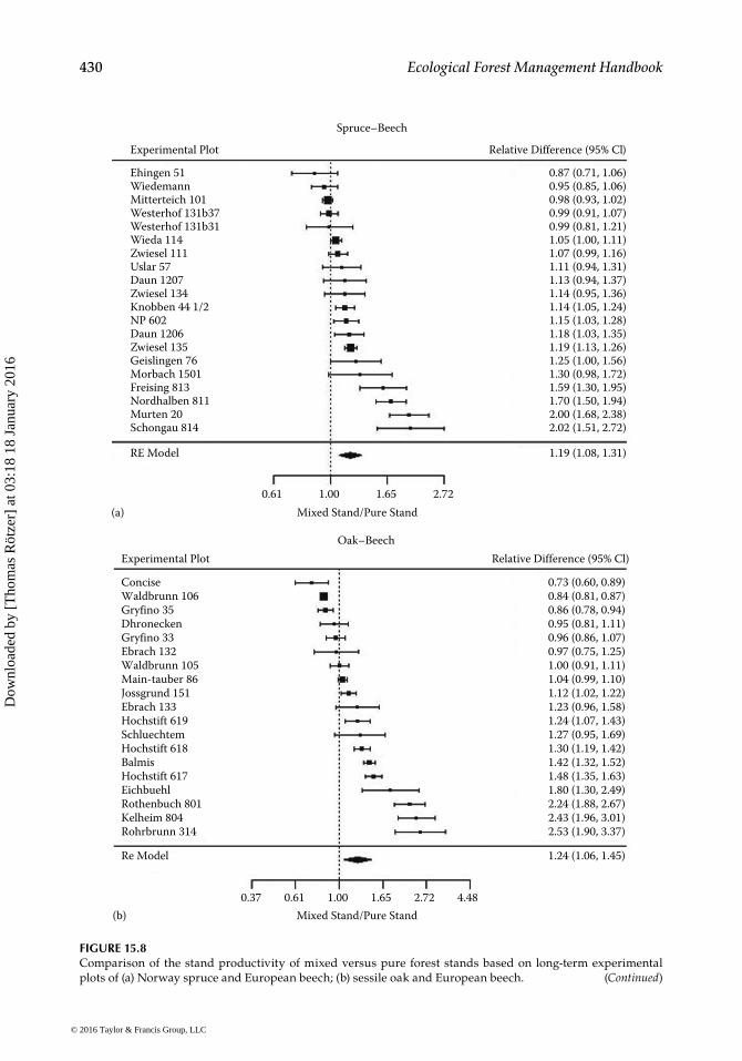
FIGURE 15.8 (Continued)Comparison of the stand productivity of mixed versus pure forest stands based on long-term experimental plots of the (c) Norway spruce, silver fir, and European beech in Germany. On average, the mixed stands pro-duce 119%, 124%, and 120%, respectively, of the weighted mean of the neighboring pure stands. All three analy-ses revealed a broad variation of mixing effects including strong underyielding and overyielding. (According to Pretzsch, H. et al., Ann. For. Sci., 67, 2010; Pretzsch, H. et al., Eur. J. For. Res., 132/2, 263, 2013a; Pretzsch, H. et al., AFJZ, 184/7/8, 177, 2013b; Pretzsch, H. et al., For. Ecol. Manage., 316, 65, 2014.)
© 2016 Taylor & Francis Group, LLC
Dow
nloa
ded
by [
Tho
mas
Röt
zer]
at 0
3:18
18
Janu
ary
2016
432 Ecological Forest Management Handbook
production when thinning even-aged pure stands or femeling mixed stands with monolay-ered canopies (Figure 15.9a and b), the productivity can decrease already after slight den-sity reductions. Thinning in even-aged mixed stands or selection cutting in uneven-aged mixed stands with deep canopy spaces (Figure 15.9c and d) causes productivity reduction not until heavy density reductions, as the trees in the medium and lower canopy layers can compensate for any losses in the upper layer. The range where productivity is rather stable, although density has been reduced, also called by Langsaeter (1941) the saddle of the density–growth relationship, is particularly wide in selection forests, as their multilayered, uneven-aged structure buffers well most structural interferences. Notice that the response pattern in Figure 15.9 represents just the general dependency between the structure and the growth. The schematically shown density–growth relationships can be modified by site conditions, species, age, and the kind of silvicultural interference.
15.6 Productivity Changes and Change Detection: Impact of Disturbance Events and Long-Term Trends on Stand Productivity
15.6.1 Long-Term Changes in Productivity
Forest ecosystems are increasingly exposed to climate change since more than 100 years (Skeffington and Wilson 1988). While only two decades ago the “Waldsterben” caused by acid rain seemed to terminate forest ecosystems (Ulrich 1990), presently phenology observa-tions (Chmielewski and Rötzer 2001), normalized differenced vegetation index (NDVI) sens-ing (Myneni et al. 2001), and inventories (Spiecker et al. 1996) indicate rather rampant than collapsing forests in Europe. Global climate change will affect forest productivity in a very-regional-specific way in the future (IPCC 2007). A crucial basis for understanding the ongoing
Even-aged, pure thinning
Min
Stand productivityStand productivityStand productivityStand productivity
Even-aged, mixedthinning, regulation
of mixing portion
Uneven-aged, mixedselection outting
Even-aged, mixedfemeling
MaxStand density(a)
Min MaxStand density(b)
Min MaxStand density(c)
Min MaxStand density(d)
1.0
FIGURE 15.9The growth resilience of stands to tree removal by thinning or losses by damage (gray silhouetted trees) increases with the deepness and layering of the canopy. Schematic representation of the strand structure (above) and the density–productivity relationship (below) of (a) an even-aged pure stand, (b) femel structured mixed stand, (c) even-aged mixed stand, and (d) uneven-aged, multilayered mixed stand. The 1.0-line (broken horizontal line) represents the productivity at maximum stand density.
© 2016 Taylor & Francis Group, LLC
Dow
nloa
ded
by [
Tho
mas
Röt
zer]
at 0
3:18
18
Janu
ary
2016
433Indicating Forest Ecosystem and Stand Productivity
changes in environmental conditions and their effect on forest stand dynamics and productiv-ity, for avoidance of negative effects by environmental policy, or for mitigating stress effects by management measures is a long-term biomonitoring. Three hundred years ago, von Carlowitz (1713) brought the idea of sustainability into forestry, and Hartig (1791, 1795), Cotta (1828), and Pfeil (1860) developed concepts for establishing this idea in forest management. In order to pro-cure growth and yield data as quantitative basis for sustainable forest management, farsighted researchers in the late 19th century started installing long-term observational and experimen-tal plots (see Verein Deutscher Forstlicher Versuchsanstalten 1873; von Ganghofer 1881).
15.6.2 Long-Term Plots as Ultimate Arbiters
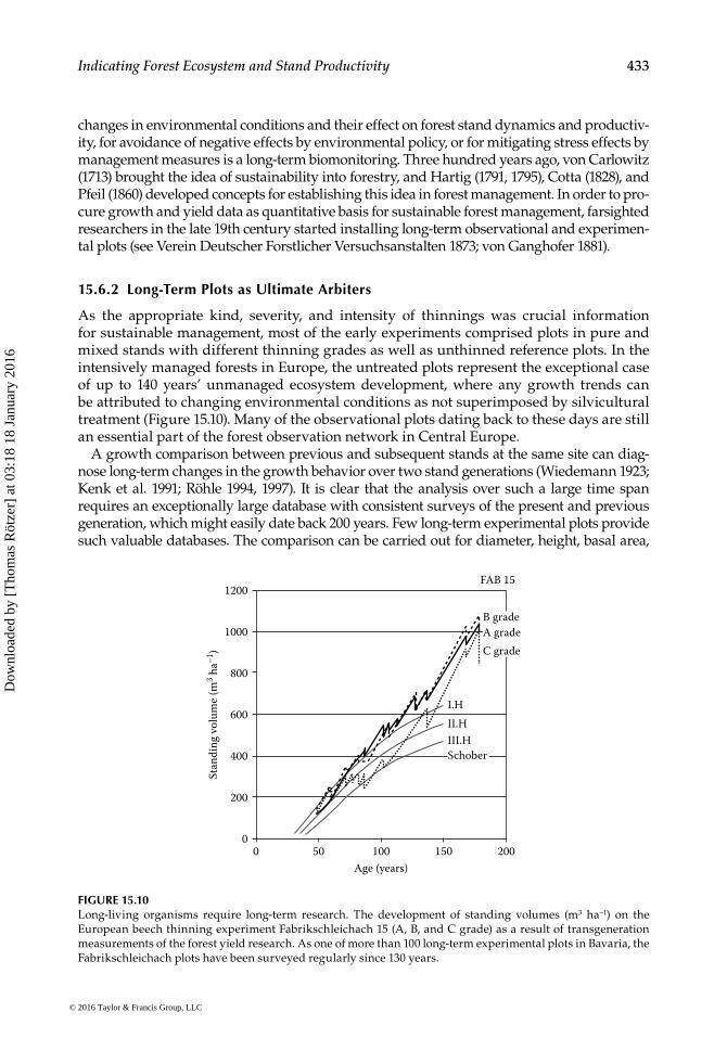
As the appropriate kind, severity, and intensity of thinnings was crucial information for sustainable management, most of the early experiments comprised plots in pure and mixed stands with different thinning grades as well as unthinned reference plots. In the intensively managed forests in Europe, the untreated plots represent the exceptional case of up to 140 years’ unmanaged ecosystem development, where any growth trends can be attributed to changing environmental conditions as not superimposed by silvicultural treatment (Figure 15.10). Many of the observational plots dating back to these days are still an essential part of the forest observation network in Central Europe.
A growth comparison between previous and subsequent stands at the same site can diag-nose long-term changes in the growth behavior over two stand generations (Wiedemann 1923; Kenk et al. 1991; Röhle 1994, 1997). It is clear that the analysis over such a large time span requires an exceptionally large database with consistent surveys of the present and previous generation, which might easily date back 200 years. Few long-term experimental plots provide such valuable databases. The comparison can be carried out for diameter, height, basal area,
00
50 100 150 200
200
Age (years)
400
600
800
1000
1200
Stan
ding
vol
ume
(m3 h
a–1)
FAB 15
B gradeA gradeC grade
I.HII.HIII.HSchober
FIGURE 15.10Long-living organisms require long-term research. The development of standing volumes (m3 ha−1) on the European beech thinning experiment Fabrikschleichach 15 (A, B, and C grade) as a result of transgeneration measurements of the forest yield research. As one of more than 100 long-term experimental plots in Bavaria, the Fabrikschleichach plots have been surveyed regularly since 130 years.
© 2016 Taylor & Francis Group, LLC
Dow
nloa
ded
by [
Tho
mas
Röt
zer]
at 0
3:18
18
Janu
ary
2016
434 Ecological Forest Management Handbook
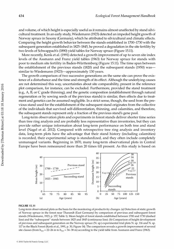
and volume, of which height is especially useful as it remains almost unaffected by stand silvi-cultural treatment. In an early study, Wiedemann (1923) detected an impeded height growth of Norway spruce in Saxony (Germany), which he attributed to silvicultural and climatic effects. Comparing the height growth behavior between the stands established in 1700–1730 with the subsequent generation established in 1825–1845, he proved a degradation in the site fertility by two levels of Schwappach’s (1890) yield tables for Norway spruce (Figure 15.11).
More recently, Kenk et al. (1991) detected a growth improvement of up to seven site index levels of the Assmann and Franz yield tables (1963) for Norway spruce for stands with poor to medium site fertility in Baden-Württemberg (Figure 15.11). The time span between the establishment of the previous stands (1820) and the subsequent stands (1950) was—similar to Wiedemann (1923)—approximately 130 years.
The growth comparison of two successive generations on the same site can prove the exis-tence of a disturbance and the time and strength of its effect. Although the underlying causes are not determined this way, uncertainties about site comparability, present in the reference plot comparison, for instance, can be excluded. Furthermore, provided the stand treatment (e.g., A, B, or C grade thinning), and the genetic composition (establishment through natural regeneration or by sowing seeds of the previous stands) is similar, then effects due to treat-ment and genetics can be assumed negligible. In a strict sense, though, the seed from the pre-vious stand used for the establishment of the subsequent stand originates from the collective of the individuals that survived self-differentiation, thinning, and calamities, and therefore, the subsequent stands represent only a fraction of the previous stand’s gene pool.
Long-term observation plots and experiments in forest stands deliver shorter time series than tree ring analysis and are probably less representative than inventories, but they can provide rather unique information about long-term performance on both tree and stand level (Nagel et al. 2012). Compared with retrospective tree ring analysis and inventory data, long-term plots have the advantage that their stand history (including calamities) is recorded, their experimental setup is standardized, and they often include completely unmanaged variants. Beginning in 1870, many long-term observational plots in Central Europe have been remeasured more than 20 times till present. As this study is based on
65
40
70 75 80 85 90 95Age (years)
1700 – 1730
Succeeding stand
Mea
n he
ight
(m) Previous stand
1825 – 1845
30
20
10
0
(a)0
0
Age (years)25 50 75 100 125 150
5
10
15
20
25
30
35
40
Dom
inan
t hei
ght (
m)
3834302622
N.sp.116
N.sp.116
N.sp.117
N.sp.117
Previous stands
Succeedingstands
(b)
FIGURE 15.11Long-term observational plots as the basis for the monitoring of productivity changes. (a) Detection of static growth of Norway spruce in the forest near Tharandt (East Germany) by comparison of previous and subsequent forest stands (Wiedemann, 1923, p. 157, Table 1). Mean height of forest stands established between 1700 and 1730 (dashed line) and the “subsequent” stands between 1825 and 1845 (continuous line). (b) Comparison of height development of previous and subsequent generation on the Norway spruce (N. sp.) experimental trial plots N. sp. 116 and N. sp. 117 in the Black Forest (Kenk et al., 1991, p. 30, Figure 14). The comparison reveals a growth improvement of several site classes (from h100 = 22–26 m to h100 = 34–38 m) according to the yield table from Assmann and Franz (1963).
© 2016 Taylor & Francis Group, LLC
Dow
nloa
ded
by [
Tho
mas
Röt
zer]
at 0
3:18
18
Janu
ary
2016
435Indicating Forest Ecosystem and Stand Productivity
long-term observational plots and exploits their information for the detection of growth trends, we briefly introduce the concept of these observation plots.
15.6.3 Current Growth Trends
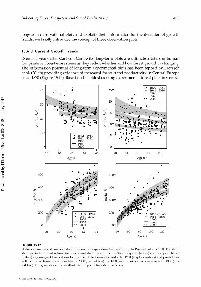
Even 300 years after Carl von Carlowitz, long-term plots are ultimate arbiters of human footprints on forest ecosystems as they reflect whether and how forest growth is changing. The information potential of long-term experimental plots has been tapped by Pretzsch et al. (2014b) providing evidence of increased forest stand productivity in Central Europe since 1870 (Figure 15.12). Based on the oldest existing experimental forest plots in Central
40
30
20
10
0
20 30
iV (m
3 ha–1
a–1)
40 50 60Age (a)
1882 – 1960
19001961– 2012
19602000
iV (m
3 ha–1
a–1)
40Age (a)
1961– 20101870 – 1960
190019602000
60 80 100 120
25
20
15
10
5
0
800
V (m
3 ha–1
)
1882 – 1960
19001961– 2012
19602000
20 30 40 50 60Age (a)
600
400
200
0
800
600
400
200
0
V (m
3 ha–1
)
1961– 20101870 – 1960
190019602000
40Age (a)
60 80 100 120
FIGURE 15.12Statistical analysis of tree and stand dynamic changes since 1870 according to Pretzsch et al. (2014). Trends in stand periodic annual volume increment and standing volume for Norway spruce (above) and European beech (below) age ranges. Observations before 1960 (filled symbols) and after 1960 (empty symbols) and predictions with our fitted linear mixed models for 2000 (dashed line), for 1960 (solid line), and as a reference for 1900 (dot-ted line). The gray-shaded areas illustrate the prediction standard error.
© 2016 Taylor & Francis Group, LLC
Dow
nloa
ded
by [
Tho
mas
Röt
zer]
at 0
3:18
18
Janu
ary
2016
436 Ecological Forest Management Handbook
Europe, this study showed that currently, the dominant tree species Norway spruce and European beech exhibit significantly faster tree growth (+32%–77%), stand volume growth (+10%–30%), and standing stock accumulation (+6%–7%) than in 1960. Stands still follow similar general allometric rules, but proceed more rapidly through usual trajectories. As forest stands develop faster, tree numbers are currently 17%–20% lower than in past same-aged stands. Self-thinning lines remain constant, while growth rates increase indicating that the stock of resources has not changed, while growth velocity and turnover have altered. Statistical analyses of the experimental plots, and application of an ecophysiologi-cal model, suggest that mainly the rise in temperature and extended growing seasons contribute to increased growth acceleration, particularly on fertile sites.
Especially, untreated, so-called 0 plots or reference plots are indispensable as they reflect just the effect of environmental changes on stand dynamics. They exclude silvicultural effects, for example, spacing, thinning, fertilization, and breeding that confound environ-mental effects when studied on the basis of inventories in managed stands. While long-term observational plots served mainly for quantifying growth and yield in the past, they address a much broader scope of forest functions and services at present and in the future (Burkhart and Temesgen 2014). While countries with observational plots dating far back should maintain and update them, countries with sustainable forestry just emerging should establish networks for long-term biomonitoring of forest components, structure, and functioning. Even 300 years after von Carlowitz (1645–1714) proposed the concept of sustainable forests by publishing Sylvicultura Oeconomica (von Carlowitz 1713), long-term plots remain the ultimate arbiters of human footprints on forest ecosystems.
15.7 Integration of Indicator Systems into Forest Management
15.7.1 Productivity Regulation as a Basis for Many Other Forest Functions and Services
Because of their size, firm position, and longevity, trees are the founder species in ecosys-tems (Whitham et al. 2006). Their morphology and structure determine the living condi-tions of many ecosystem characteristics, their functions, and many services beyond the wood and timber quality (Hector and Bagchi 2007). By the shading effect of their crowns and the water uptake of their roots, trees influence the light and water supply and thus the habitats of flora and fauna in their surroundings.
Therefore, forest inventories, especially when based on fixed grid points, including spatial explicit tree and stand records, and when repeated over time, comprise valuable and hardly extracted aspects of functional, compositional, and structural diversity. The commonly mea-sured annual growth rate not only provides information about the allowable cut but also correlates closely with the leaf biomass turnover, which is essential for feeding all herbivores and decomposers. Tree size and structure not only determines the standing stock and wood quality but also forms the habitat of many animals like birds, bats, and spiders.
15.7.2 Stand Productivity and Sustainable Productivity at the Enterprise Level
The mean annual volume increment (MAI) and mean standing volume stock (V) that allows this MAI are the most fundamental indicators for any planning and management. They represent the potential mean productivity and mean standing volume within a
© 2016 Taylor & Francis Group, LLC
Dow
nloa
ded
by [
Tho
mas
Röt
zer]
at 0
3:18
18
Janu
ary
2016
437Indicating Forest Ecosystem and Stand Productivity
time span from stand establishment to culmination of the MAI (rotation period) in age-class forest and the long-term mean productivity and standing stock in uneven-aged forest, such as selection forest systems. Both indicators depend mainly on the prevailing site conditions, the chosen tree species, and occurring disturbances. MAI and V can be derived for both stand and management block level based on, for example, observational plots, yield tables, or stand simulators. MAI indicates the level of the potential sustain-able annual cut.
In contrast, the actually possible annual cut is induced in the course of silvicultural plan-ning by assessing the appropriate treatment and resulting annual cut at the individual stand, stand type, or stratum level. However, this silviculturally derived possible annual cut reflects just the possible quantity of logging that might considerably differ from the long-term sustainable cut aimed at on overall enterprise level. A high stock of old stands may suggest a far-above-average annual cut for the coming planning period, which might be distributed over a longer time span in order to avoid a long time period of under-average annual cut.
15.7.3 Productivity Regulation in Forest Practices
Based on the information about the potential and actual annual cut on the one hand, and the long-term objective on the other hand, forest management deduces a long-term sus-tainable cut that might considerably differ from both potential and annual. The main rea-son for such deviations is, beside any legal, political, or ecological restrictions, that the planning normally aims at achieving a stable annual cut that can be realized continuously over a long or even infinite time span without exploiting, but only sustainably removing the mean annual increment.
Especially when forest management planning aims at equalization of a so far uneven age-class distribution, replacement of pure by mixed-species stands, or transition from age-class to uneven-aged management, simulation models can support the decision mak-ing. They show the long-term effect of various silvicultural options and help to find out which set of silvicultural prescriptions (thinning, mixing, final cutting, regeneration) is necessary for achieving a target long-term annual cut and respective standing stock. The recursive planning process includes the provisional selection of silvicultural measures for all planning units → upscaling of the resulting long-term development and annual cut → comparison of the resulting long-term development and annual cut with the target state of the management block → modification of silvicultural measures for selected planning units in order to better arrive at the target state → upscaling of the modified treatments with respect to the long-term development at the overall management block level. It is much easier and more flexible when based on simulation models compared with classical approaches based on normal forest assumptions, yield tables, and formulas for indicating the sustainable annual cut.
A combined use of simulation models for strategic and recursive planning and long-term permanent inventory plots for model control is common in modern planning. Silvicultural measures, which strongly affect the standing stock, volume growth, and productivity at the individual stand level and the sustainable cut at the enterprise level on the long term, are in particular the amount of final cutting, thinning, and regeneration. Long-term effects have furthermore species and provenance choice, species mixing, mixing regulation, wild repellent, and mechanical stabilization by tending and thinning.
The long-term annual cut as deduced by recursive planning at stand and overall enter-prise level is the most relevant indicator for sustainable forest management.
© 2016 Taylor & Francis Group, LLC
Dow
nloa
ded
by [
Tho
mas
Röt
zer]
at 0
3:18
18
Janu
ary
2016
438 Ecological Forest Management Handbook
15.8 Perspectives: From Deductive to Inductive and Static to Dynamic Indications of Forest Ecosystem and Stand Productivity
Former approaches deduced forest ecosystem and stand productivity from general models, which were based on a rather small number of long-term observational plots. As examples for this approach, we introduced productivity indices, yield tables, individual tree models that were based on long-term experiments.
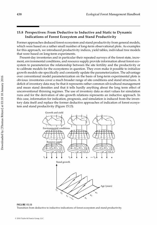
Present-day inventories and in particular their repeated surveys of the forest state, incre-ment, environmental conditions, and resource supply provide information about forest eco-system to parameterize the relationship between the site fertility and the productivity or to calibrate models for the ecosystems in question. They even make it possible to initialize growth models site specifically and constantly update the parameterization. The advantage over conventional model parameterization on the basis of long-term experimental plots is obvious: inventories cover a much broader range of site conditions and stand structures. A deficit of inventory data may be that it represents rather common silvicultural management and mean stand densities and that it tells hardly anything about the long term effect of unconventional thinning regimes. The use of inventory data as start values for simulation runs and for the derivation of site–growth relations represents an inductive approach. In this case, information for indication, prognosis, and simulation is induced from the inven-tory data itself and replace the former deductive approaches of indication of forest ecosys-tem and stand productivity (Figure 15.13).
Growth and yield
Environmental conditions
Rsource supply
Stand growth
Age (years)
tn
tn
t2
t2t3
t1
a1
a3a2
t1
FIGURE 15.13Transition from deductive to inductive indications of forest ecosystem and stand productivity.
© 2016 Taylor & Francis Group, LLC
Dow
nloa
ded
by [
Tho
mas
Röt
zer]
at 0
3:18
18
Janu
ary
2016
439Indicating Forest Ecosystem and Stand Productivity
References
Ajtay, G.L., P. Ketner, and P. Duvigneaud. 1979. Terrestrial primary production and phytomass. Glob. Carbon Cycle 13: 129–182.
Assmann, E. 1970. The Principles of Forest Yield Study. New York: Pergamon Press, p. 473.Assmann, E. and F. Franz. 1963. Vorläufige Fichten-Ertragstafel für Bayern. München, Germany: Forstl
Forschungsanst München, Inst Ertragskd, 104p.Batho, A. and O. Garcia. 2006. De Perthuis and the origins of site index: A historical note. FBMIS
1: 1–10.Baur von, F. 1876. Die Fichte in Bezug auf Ertrag, Zuwachs und Form. Berlin, Germany: Springer-Verlag, 58p.Beer, C., M. Reichstein, E. Tomelleri et al. 2010. Terrestrial gross carbon dioxide uptake: Global dis-
tribution and covariation with climate. Science 329/5993: 834–838.Bettinger, P., K. Boston, J.P. Siry et al. 2009. Forest Management Planning. Amsterdam, the Netherlands:
Elsevier.Bresinsky, A., C. Körner, J.W. Kadereit et al. 2008. Strasburger Lehrbuch der Botanik. Heidelberg,
Germany: Auflage. Spektrum Akademischer Verlag, p. 36.Brünig, E.F. 1971. Forstliche Produktionslehre. Bern, Switzerland: Europ Hochschulschr, Reihe XXV,
Verlag Herbert Lang, Bern und Peter Lang, Frankfurt, 318p.Bruscheck, G.J. 1994. Waldgebiete und Waldbrandgeschehen in Brandenburg im Trockensommer
1992. PIK-Report 2: 245–264.Buchmann, N. and E.D. Schulze. 1999. Net CO2 and H2O fluxes of terrestrial ecosystems. Glob.
Biogeochem. Cycles 13/3: 751–760.Burkhart, H. and H. Temesgen. 2014. Forest observational studies: Data sources for analysing forest
structure and dynamics. For. Ecol. Manage.316: 147.Cajander, A.K. 1926. The theory of forest types. Acta forestalia fennica 29: 108.Carvalhais, N., M. Forkel, M. Khomik et al. 2014. Global co-variation of carbon turnover times in
terrestrial ecosystems with climate. Nature 514: 213–217.Chapin, F.S., G.M. Woodwell, J.T. Randerson et al. 2006. Reconciling carbon-cycle concepts, termi-
nology, and methods. Ecosystems 9/7: 1041–1050.Chmielewski, F.M. and T. Rötzer. 2001. Response of tree phenology to climate change across Europe.
Agric. For. Meteorol. 108(2): 101–112.Crutzen, P.J. 2002. Geology of mankind. Nature 415: 23.Dale, V.H. and S.C. Beyeler. 2001. Challenges in the development and use of ecological indicators.
Ecol. Indic. 1: 3–10.Davis, K.P. 1966. Forest Management. New York McGraw-Hill Book Company.del Río, M., S. Condés, and H. Pretzsch 2014a. Analyzing size-symmetric versus size-asymmetric
and intra-versus inter-specific competition in beech (Fagus sylvatica L.) mixed stands. For. Ecol. Manage. 325: 90–98.
del Río, M., G. Schütze, and H. Pretzsch 2014b. Temporal variation of competition and facilitation in mixed species forests in Central Europe. Plant Biol. 16: 166–176.
Delucia, E.H., J.E. Drake, R.B. Thomas et al. 2007. Forest carbon use efficiency: Is respiration a con-stant fraction of gross primary production? Glob. Change Biol. 13: 1157–1167.
Dobbertin, M. 2005. Tree growth as indicator of tree vitality and of tree reaction to environmental stress: A review. Eur. J. For. Res.124/4: 319–333.
Dudley, N. and S. Stolton. 2003. Running Pure: The Importance of Forest Protected Areas to Drinking Water. Gland, Switzerland: World Bank/WWF Alliance for Forest Conservation and Sustainable Use.
Eichhorn, F. 1902. Ertragstafeln für die Weißtanne. Berlin, Germany: Verlag Julius Springer.Fang, J., T. Kato, Z. Guo et al. 2014. Evidence for environmentally enhanced forest growth. PNAS
111/26: 9527–9532.FAO 2012. Global ecological zones for FAO Forest reporting: 2010 Update. Forest resources assessment
working paper 179. Rome, Italy: Food and Agriculture Organization of the United Nations.
© 2016 Taylor & Francis Group, LLC
Dow
nloa
ded
by [
Tho
mas
Röt
zer]
at 0
3:18
18
Janu
ary
2016
440 Ecological Forest Management Handbook
Fernández-Martínez, M., S. Vicca, I.A. Janssens et al. 2014. Spatial variability and controls over biomass stocks, carbon fluxes, and resource-use efficiencies across forest ecosystems. Trees 28/2: 597–611.
Field, C.B. and M.R. Raupach. 2004. The Global Carbon Cycle: Integrating Humans, Climate, and the Natural World (SCOPE 62). Island Press.
Forrester, D.I., J. Bauhus, A.L. Cowie, and J.K. Vanclay. 2006. Mixed-species plantations of Eucalyptus with nitrogen-fixing trees: A review. For. Ecol. Manage. 233: 211–230.
Gehrhardt, E. 1923. Ertragstafeln für Eiche, Buche, Tanne, Fichte und Kiefer. Berlin, Germany: Verlag Julius Springer.
Gough, A.D., J.L. Innes, and S.D. Allen. 2008. Development of common indicators of sustainable for-est management. Ecol. Indic. 8: 425–430.
Griess, V.C. and T. Knoke. 2011. Growth performance, windthrow, and insects: Meta-analyses of parameters influencing performance of mixed-species stands in boreal and northern temper-ate biomes. Can. J. For. Res 41: 1141–1158.
Hanewinkel, M. 2001. Neuausrichtung der Forsteinrichtung als strategisches Management Instrument. AFJZ 172: 203–211.
Hartig, G.L. 1791. Anweisung zur Holzzucht für Förster. Marburg, Germany: Neue Akademische Buchhandlung.
Hartig, G.L. 1795. Anweisung zur Taxation der Forste oder zur Bestimmung des Holzertrags der Wälder. Wiesbaden, Germany: Georg-Ludwig-Hartig-Stiftung.
Hector, A. and R. Bagchi. 2007. Biodiversity and ecosystem multifunctionality. Nature 448: 188–190.Heyer, G. 1845. Wedekinds Neue Jahrb. Climate Change: The Scientific Basis. Cambridge University
Press, Cambridge. 30: 1–127.Heyer, G. 1852. Über die Ermittlung der Masse, des Alters und des Zuwachses der Holzbestände. Dessau,
Germany: Verlag Katz.Ito, A. 2011. A historical meta‐analysis of global terrestrial net primary productivity: Are estimates
converging? Glob. Chang. Biol. 17/10: 3161–3175.IPCC. 2001. http://www.ipcc.ch/ipccreports/tar/wg1/099.htm#tab32 (accessed November 4,
2014).IPCC. 2006. Guidelines for national greenhouse gas inventories. Vol. 4 Agriculture, Forestry and
Other Land Use, Prepared by the National Greenhouse Gas Inventories Programme. In: Eggleston, S., Buendia, L., Miwa, K., Ngara, T., and Tanabe, K. (eds.). Kanagawa, Japan: Institute for Global Environmental Strategies.
IPCC. 2007. Fourth Assessment Report: Climate Change 2007. Working Group I Report. The Physical Science Basis. Geneva, Switzerland, 104p.
Jørgensen, S.E., B. Burkhard, and F. Müller. 2013. Twenty volumes of ecological indicators - An accounting short review. Ecol. Indic. 28: 4–9.
Judeich, F. 1871. Die Forsteinrichtung. Dresden, Germany: Schönfelds Verlagsbuchhandlung.Kahn, M. 1994. Modellierung der Höhenentwicklung ausgewählter Baumarten in Abhängigkeit
vom Standort. Forstliche Forschungsberichte München 141: 221.Kenk, G., H. Spiecker, and G. Diener. 1991. Referenzdaten zum Waldwachstum. Karlsruhe, Germany:
Kernforschungszentrum Karlsruhe, KfK-PEF 82, 59p.Knoke, T., T. Schneider, A. Hahn et al. 2012. Forstbetriebsplanung als Entscheidungshilfe. Stuttgart,
Germany: Ulmer.Kramer, H. 1988. Waldwachstumslehre. Berlin, Germany: Paul Parey Verlag.Lal, P., J. Alavalapati, M. Marinescu et al. 2011. Developing sustainability indicators for woody bio-
mass harvesting in the United States. J. Sust. For. 30: 736–755.Landsberg, J.J. 1986. Physiological Ecology of Forest Production. London, UK: Academic Press.Landsberg, J.J. and R.H. Waring. 1997. A generalised model of forest productivity using simpli-
fied concepts of radiation-use efficiency, carbon balance and partitioning. For. Ecol. Mod. 95: 209–228.
Langsaeter, A. 1941. Om tynning i enaldret granog furuskog Maddel. Det Norske Skogforoksvesen 8: 131–216.
© 2016 Taylor & Francis Group, LLC
Dow
nloa
ded
by [
Tho
mas
Röt
zer]
at 0
3:18
18
Janu
ary
2016
441Indicating Forest Ecosystem and Stand Productivity
Larcher, W. 2003. Physiological Plant Ecology: Ecophysiology and Stress Physiology of Functional Groups. Berlin, Germany: Springer Verlag.
Luyssaert, S., I. Inglima, M. Jung et al. 2007. CO2 balance of boreal, temperate, and tropical forests derived from a global database. Glob. Chang. Biol. 13/12: 2509–2537.
Lyr, H, H.J. Fiedler, and W. Tranquillini. 1992. Physiologie und Ökologie der Gehölze. Jena, LA: G. Fischer Verlag.
Mantel, W. 1949. Forsteinrichtungslehre. Hamburg, Germany: Neumann-Neudamm.Marland, G. and B. Schlamadinger. 1997. Forests for carbon sequestration or fossil fuel substitution?
A sensitivity analysis. Biomass Bioenergy 13/6: 389–397.Martonne de, E. 1926. Une novelle fonction climatologique: L’indice d’aridité. La Météorologie 21:
449–458.Matyssek, R., J. Fromm, H. Rennenberg et al. 2010. Biologie der Bäume. Stuttgart, Germany: Verlag
Eugen Ulmer.McMahon, S.M., G.G. Parker, and D.R. Miller. 2010. Evidence for a recent increase in forest growth.
PNAS 107/8: 3611–3615.Michaletz, S.T., D. Cheng, A.J. Kerkhoff et al. 2014. Convergence of terrestrial plant production across
global climate gradients. Nature 512: 39–43.Mitscherlich, G. 1970. Wald, Wachstum und Umwelt. 1. Band, Form und Wachstum von Baum und
Bestand. Frankfurt am Main, Germany: JD Sauerländer’s Verlag.Molden, D., H. Murray-Rust, R. Sakthivadivel, and I. Makin. 2003. A water-productivity framework
for understanding and action. Water Prod. Agric.: Limits Opport. Impr. 1: 1–18.Monteith, J.L. 1975. Vegetation and the Atmosphere, Vol. 1, Principles, Vol. 2, Case Studies. London, UK:
Academic Press.Moosmayer, H.U. and W. Schöpfer. 1972. Beziehungen zwischen Standortsfaktoren und
Wuchsleistung der Fichte. AFJZ 143/10: 203–215.Morin, X., L. Fahse, M. Scherer-Lorenzen et al. 2011. Tree species richness promotes produc-
tivity in temperate forests through strong complementarity between species. Ecol. Letters 14: 1211–1219.
Myneni, R.B., J. Dong, C.J. Tucker et al. 2001. A large carbon sink in the woody biomass of northern forests. Proc. Natl. Acad. Sci. 98(26): 14784–14789.
Nagel, J., H. Spellmann, and H. Pretzsch. 2012. Zum Informationspotenzial langfristiger forstli-cher Versuchsflächen und periodischer Waldinventuren für die waldwachstumskundliche Forschung. AFJZ 183, 111–116.
Noss, R.F. 1990. Indicators for monitoring biodiversity: A hierarchical approach. Conserv. Biol. 4/4: 355–364.
Oesten, G. and A. Roeder. 2012. Management von Forstbetrieben, Band I-III, Institut für Forstökonomie der Universität Freiburg, www.ife.uni-freiburg.de/lehre/lehrbuch-1 respec-tively lehrbuch-2 und -3, Volume I-III: 383p, 365p, and 291p.
Oliver, C.D. and B. Larson. 1996. Forest Stand Dynamics. New York: John Wiley & Sons Inc., 520p.Pan, Y., R.A. Birdsey, J. Fang et al. 2011. A large and persistent carbon sink in the world’s forests.
Science 333/6045: 988–993.Paterson, S.S. 1956. The Forest Area of the World and Its Potential Productivity. Sweden: The Royal
University of Göteborg, Sweden, Department of Geography, Lerums Boktryckeri, 216p.Paquette, A. and C. Messier. 2011. The effect of biodiversity on tree productivity: From temperate to
boreal forests. Glob. Ecol. Biogeogr 20/1: 170–180.Perthuis de Laillevault, R. 1803. Traité de l’aménagement et de la restauration des bois et forêts de la France.
Paris, France: Madame Huzard.Pfeil, W. 1860. Die deutsche Holzzucht. Leipzig, Germany: Verlag Baumgartner, 551p.Piao, S., S. Sitch, P. Ciais et al. 2013. Evaluation of terrestrial carbon cycle models for their response
to climate variability and to CO2 trends. Glob. Chang. Biol. 19: 2117–2132.Piotto, D. 2008. A meta-analysis comparing tree growth in monocultures and mixed plantations.
For. Ecol. Manage.255: 781–786.
© 2016 Taylor & Francis Group, LLC
Dow
nloa
ded
by [
Tho
mas
Röt
zer]
at 0
3:18
18
Janu
ary
2016
442 Ecological Forest Management Handbook
Pressler, M. 1877. Forstliche Zuwachs-, Ertrags- und Bonitierungs-Tafeln mit Regeln und Beispielen, 2nd edn. Tharandt, Germany: Selfpubl.
Pretzsch, H. 1995. Zum Einfluß des Baumverteilungsmusters auf den Bestandeszuwachs. AFJZ 166/9/10: 190–201.
Pretzsch, H. 1996. Growth Trends of Forests in Southern Germany: In Growth Trends in European Forests. Berlin, Heidelberg: Springer Verlag.
Pretzsch, H. 2003. The elasticity of growth in pure and mixed stands of Norway spruce (Picea abies (L.) Karst.) and common beech (Fagus sylvatica L.). J. For. Sci. 49(11): 491–501.
Pretzsch, H. 2005a. Diversity and productivity in forests. In: Scherer-Lorenzen, M., Körner, C., and Schulze, E.D. (eds.). Forest Diversity and Function: Ecol Studies. Berlin, Germany: Springer-Verlag, 176p.
Pretzsch, H. 2005b. Stand density and growth of Norway spruce (Picea abies (L.) Karst.) and European beech (Fagus sylvatica L.). Evidence from long-term experimental plots. Eur. J. For. Res124: 193–205.
Pretzsch, H. 2009. Forest Dynamics, Growth and Yield. Berlin, Heidelberg: Springer Verlag.Pretzsch, H., P. Biber, and J. Ďurský. 2002. The single tree based stand simulator SILVA. Construction,
application and evaluation. For. Ecol. Manage.162: 3–21.Pretzsch, H., P. Biber, G. Schütze et al. 2014a. Changes of forest stand dynamics in Europe. Facts
from long-term observational plots and their relevance for forest ecology and management. For. Ecol. Manage.316: 65–77.
Pretzsch, H., P. Biber, G. Schütze et al. 2014b. Forest stand growth dynamics in Central Europe have accelerated since 1870. Nat. Commun. 5: 4967. DOI:10.1038/ncomms5967.
Pretzsch, H., K. Bielak, and J. Block et al. 2013a. Productivity of pure versus mixed stands of oak (Quercus petraea (MATT.) LIEBL. and Quercus robur L.) and European beech (Fagus sylvatica L.) along an ecological gradient. Eur. J. For. Res 132/2: 263–280.
Pretzsch, H., K. Bielak, A. Bruchwald et al. 2013b. Species results from long-term experiments. AFJZ 184/7/8: 177–196. [In German with English summary].
Pretzsch, H., J. Block, J. Dieler et al. 2010. Comparison between the productivity of pure and mixed stands of Norway spruce and European beech along an ecological gradient. Ann. For. Sci. 67(7): 712.
Pretzsch, H., J. Dieler, T. Seifert et al. 2012. Climate effects on productivity and resource use effi-ciency of Norway spruce (Picea abies [L.] Karst.) and European beech (Fagus sylvatica [L.]) in stands with different spatial mixing patterns. Trees 26: 1343–1360.
Pretzsch, H., R. Grote, B. Reineking et al. 2008. Models for forest ecosystem management: A European perspective. Ann. Bot. 101: 1065–1087.
Pretzsch, H., G. Schütze, and E. Uhl. 2013. Resistance of European tree species to drought stress in mixed versus pure forests: Evidence of stress release by inter-specific facilitation. Plant Biol.15: 483–495.
Quéré, C.L., R.J. Andres, T. Boden et al. 2013. The global carbon budget 1959–2011. Earth Syst. Sci. Data 5/1: 165–185.
Röhle, H. 1994. Zum Wachstum der Fichte auf Hochleistungsstandorten in Südbayern. München, Germany: Ertragskundliche Auswertung langfristig beobachteter Versuchsreihen unter besonderer Berücksichtigung von Trendänderungen im Wuchsverhalten. Habil Forstwiss Fak, LMU München, 249p.
Röhle, H. 1997. Änderung von Bonität und Ertragsniveau in südbayerischen Fichtenbeständen. AFJZ 168(6/7): 110–114.
Rötzer, T., T. Seifert, and H. Pretzsch 2009. Modelling above and below ground carbon dynamics in a mixed beech and spruce stand influenced by climate. Eur. J. For. Res. 128: 171–182.
Roy, J., H.A. Mooney, and B. Saugier. 2001. Terrestrial Global Productivity. Academic Press.Saugier, B., J. Roy, and H.A. Mooney. 2001. Estimations of global terrestrial productivity: Converging
toward a single number? In: Roy, J., Saugier, B., Mooney, H.A. (eds.). Terrestrial Global Productivity. San Diego, CA: Academic Press.
© 2016 Taylor & Francis Group, LLC
Dow
nloa
ded
by [
Tho
mas
Röt
zer]
at 0
3:18
18
Janu
ary
2016
443Indicating Forest Ecosystem and Stand Productivity
Schellnhuber, H.J. 1999. ‘Earth system’ analysis and the second Copernican revolution, Nature 402: 19–23.
Schultz, J. 2008. Die Ökozonen der Erde, Vol. 4, völlig neu bearbeitete Auflage. Stuttgart, Germany: Ulmer.
Schwappach, A. 1890. Wachstum und Ertrag normaler Fichtenbestände. Berlin, Germany: Verlag Julius Springer, 100p.
Sitch, S., B. Smith, I.C. Prentice et al. 2003. Evaluation of ecosystem dynamics, plant geography and terrestrial carbon cycling in the LPJ dynamic global vegetation model. Glob. Chang. Biol. 9: 161–185.
Skeffington, R.A. and E.J. Wilson. 1988. Excess nitrogen deposition: Issues for consideration. Environ. Poll. 54: 159–184.
Smith, T.M. and R.L. Smith. 2009. Ökologie. München, Germany: Addison-Wesley Verlag; 6. Auflage.Speidel, G. 1972. Planung im Forstbetrieb. Hamburg, Germany: Verlag Paul Parey.Spiecker, H., K. Mielikäinen, M. Köhl et al. 1996. Growth Trends in European Forests. Europ For Inst,
Res Rep 5, Heidelberg, Germany: Springer-Verlag.Steffen, W., I. Noble, J. Canadell et al. 1998. The terrestrial carbon cycle: Implications for the Kyoto
Protocol. Science 280: 1393–1394.Turner, D.P., W.D. Ritts, W.B. Cohen et al. 2005. Site‐level evaluation of satellite‐based global ter-
restrial gross primary production and net primary production monitoring. Glob. Chang. Biol. 11/4: 666–684.
Ulrich, B. 1990. Waldsterben: Forest decline in West Germany. Environ. Sci. Technol. 24(4): 436–441.Vanclay, J.K. 1994. Modelling Forest Growth and Yield: Applications to Mixed Tropical Stands. Wallingford,
UK: CAB International.Verein Deutscher Forstlicher Versuchsanstalten. 1873. Anleitung für Durchforstungsversuche. In:
von Ganghofer, A. (ed.) (1884) Das Forstliche Versuchswesen. Augsburg, Germany: Schmid‘sche Buchhandlung, vol. 2, pp. 247–253.
Vile, D., B. Shipley, and E. Garnier. 2006. Ecosystem productivity can be predicted from potential relative growth rate and species abundance. Ecol. Lett. 9/9: 1061–1067.
von Baur, F. 1876. Die Fichte in Bezug auf Ertrag, Zuwachs und Form. Berlin, Germany: Springer-Verlag, 58p.von Carlowitz, H.C. 1713. Sylvicultura Oekonomica oder Haußwirthliche Nachricht und Naturmäßige
Anweisung zur wilden Baum-Zucht. Leipzig, Germany: JF Braun.von Cotta, H. 1828. Anweisung zum Waldbau. Leipzig, Germany: Arnoldische Buchhandlung.von Gadow, K. 2005. Forsteinrichtung. Analyse und Entwurf der Waldentwicklung. Göttingen, Germany:
Univ-Verlag Göttingen, 342p.von Gadow, K. 2013. Messung und Modellforschung-Grundlagen der Forsteinrichtung. AFJZ
184/7/8: 143–158.von Ganghofer, A. 1881. Das Forstliche Versuchswesen. Augsburg, Germany, 505p.Waide, R.B., M.R. Willig, C.F. Steiner et al. 1999. The relationship between productivity and species
richness. Ann. Rev. Ecol. Syst. 257–300.Wang, J., P.M. Rich, K.P. Price et al. 2004. Relations between NDVI and tree productivity in the cen-
tral Great Plains. Int. J. Remote Sens.25/16: 3127–3138.Weiskittel, A.R., N.L. Crookston, and P.J. Radtke. 2011. Linking climate, gross primary productivity,
and site index across forests of the western United States. Can. J. For. Res 41: 1710–1721.Wiedemann, E. 1923. Zuwachsrückgang und Wuchsstockungen der Fichte in den mittleren und
unteren Höhenlagen der sächsischen Staatsforsten. Tharandt, Germany: Kommissionsverlag W Laux, 181p.
Wiedemann, E. 1943. Kiefern-Ertragstafel für mäßige Durchforstung, starke Durchforstung und Lichtung, In: Wiedemann E (1948) Die Kiefer 1948. Hannover, CO: Verlag M and H Schaper.
Whitham, T.G., J.K. Bailey, J.A. Schweitzer et al. 2006. A framework for community and ecosystem genetics: From genes to ecosystems. Nat. Gen. 7: 510–523.
Whittaker, R.H. and G.E. Likens. 1973. Primary production: The biosphere and man. Human Ecology 1/4: 357–369.
© 2016 Taylor & Francis Group, LLC
Dow
nloa
ded
by [
Tho
mas
Röt
zer]
at 0
3:18
18
Janu
ary
2016

444 Ecological Forest Management Handbook
Wykoff, W.R., N.L. Crookston, and A.R. Stage. 1982. User’s guide to the stand prognosis model. Ogden, UT: U.S. Forest Serv, Gen Techn Rep INT-133.
Wykoff, W.R. and R.A. Monserud. 1988. Representing site quality in increment models: A com-parison of methods. In: Ek, A.R., Shifley, S.R, and Burk, T.E. (eds.) Proceedings of the IUFRO Conference, August 1987, Gen Tech Rep NC-120, Minneapolis, MN.
Yaffee, S.L. 1999. Three faces of ecosystem management. Conser. Biol. 13: 713–725.Zhang, Y., H.Y. Chen, and P.B. Reich. 2012. Forest productivity increases with evenness, species rich-
ness and trait variation: A global meta-analysis. J. Ecol. 100/3: 742–749.Zeide, B. 2001. Thinning and growth: A full turnaround. J. For. 99: 20–25.Zeide, B. 2002. Density and the growth of even-aged stands. For. Sci. 48: 743–754.Zeide, B. 2003. The U-approach to forest modeling. Can. J. For. Res 33: 480–489.
© 2016 Taylor & Francis Group, LLC
Dow
nloa
ded
by [
Tho
mas
Röt
zer]
at 0
3:18
18
Janu
ary
2016