Embed Size (px)
Citation preview
Chapter 12
SUPERVISED LEARNINGCategorization, Decision Trees
Part 1
Cios / Pedrycz / Swiniarski / KurganCios / Pedrycz / Swiniarski / Kurgan

© 2007 Cios / Pedrycz / Swiniarski /
Kurgan
Outline
• What is Inductive Machine Learning?- Categorization of ML Algorithms
- Generation of Hypotheses
• Decision Trees
• Rule Algorithms - DataSqueezer
• Hybrid Algorithms - CLIP4- Set Covering algorithm

© 2007 Cios / Pedrycz / Swiniarski /
Kurgan
What is Inductive Machine Learning?
How do we understand learning?
We define it as the ability of an agent (like an algorithm) to improve its own performance based on past experience.

© 2007 Cios / Pedrycz / Swiniarski /
Kurgan
What is Inductive Machine Learning?
Machine Learning (ML) can be also defined as the ability of a computer program:
• to generate a new data structure that is different from an old one, like production if…then… rules from input numerical or nominal data
© 2007 Cios / Pedrycz / Swiniarski /
Kurgan
What is Inductive Machine Learning?
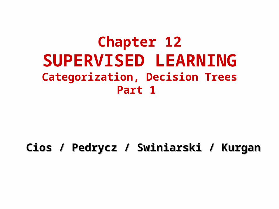
• The key concept in inductive ML is that of a hypothesis, which is generated by a given algorithm
• A hypothesis approximates some concept • We assume that only a teacher/oracle knows the true
meaning of a concept and describes the concept, via means of examples, to a learner whose task is to generate a hypothesis that best approximates the concept
Example: concept of a “pneumonia” can be described by (high fever, pneumonia)(weak, pneumonia)

© 2007 Cios / Pedrycz / Swiniarski /
Kurgan
What is Inductive Machine Learning?
Inductive ML algorithms generate hypotheses that approximate concepts;
hypotheses are often expressed in the form of production rules, and we say that
the rules “cover” the examples.
An example is covered by a rule when it satisfies all conditions of the IF part of the rule.

© 2007 Cios / Pedrycz / Swiniarski /
Kurgan
What is Inductive Machine Learning?
Any inductive ML process is broken into two phases:
• Learning phase, where the algorithm analyzes the training data and recognizes similarities among data objects. The result of this analysis is. For example, generation of a tree, or a set of production rules.
• Testing phase, where the rules are evaluated on new data, and when some performance measures may be computed.

© 2007 Cios / Pedrycz / Swiniarski /
Kurgan
What is Inductive Machine Learning?
Some ML algorithms, such as decision trees or rule learners, are able to generate explicit rules, which can be inspected, learned from, or modified by users
This is an important advantage of this type of ML algorithms over many other data mining methods.
© 2007 Cios / Pedrycz / Swiniarski /
Kurgan
What is Inductive Machine Learning?
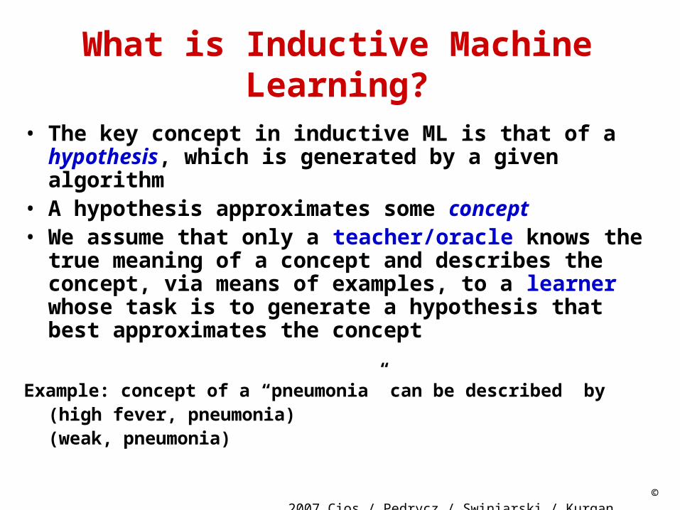
There are several levels (a pyramid) of knowledge:• Data• Warehouse
(carry original information)• (Extracted) Databases
(contain only useful information)• Knowledge / Information
(generated from a database, e.g. a set of rules)• Meta-knowledge
(knowledge about knowledge)

© 2007 Cios / Pedrycz / Swiniarski /
Kurgan
Categorization of ML algorithms
ML algorithms operate in one of two modes:
1. Supervised Learning / learning from examples (all examples have the corresponding target class)
2. Unsupervised Learning / learning from observation (examples/patterns/instances do not have target class)

© 2007 Cios / Pedrycz / Swiniarski /
Kurgan
Categorization of ML algorithms
Unsupervised Learning: learning system on its own needs to discover “classes” in the data by discovering common unifying properties (with none, or minimal help from the user)
• Clustering – finding groups of “similar” examples
• Association Rules - generation of rules describing frequently co-occurring items

© 2007 Cios / Pedrycz / Swiniarski /
Kurgan
Categorization of ML algorithms
Incremental vs. non-incremental
In non-incremental learning all of the training examples are presented simultaneously (as a batch file) to the algorithm.
In incremental learning the examples are presented one at a time (or in groups) and the algorithm improves its performance based on the new examples without the need of re-training.
Most ML algorithms are non-incremental.

© 2007 Cios / Pedrycz / Swiniarski /
Kurgan
Categorization of ML algorithms
Any supervised learning algorithm must be provided with a training data set. Let us assume that such a set S consists of M training data pairs, belonging to C classes:
S = {(xi cj) | i = 1,...,M; j = 1,...,C}
the training data pairs are often called examples, where xi is an n-dimensional pattern vector whose components are its features/attributes, and cj is a known class.
The mapping function f, c = f(x), is not known.

© 2007 Cios / Pedrycz / Swiniarski /
Kurgan
Categorization of ML algorithms
Supervised Learning: known as inductive ML or learning from examples. The user, serving role of the teacher, provides examples describing each class/concept.
• Rote learning – the system is “told” the correct rules
• Learning by analogy – system is taught the correct
response to a similar task; system needs to adapt to the new situation
© 2007 Cios / Pedrycz / Swiniarski /
Kurgan
Categorization of ML algorithms
Case-based learning - the learning system stores all the cases it has studied so far along with their outcomes. When a new case is encountered the system tries to adapt to this new case by comparing with the stored previous behavior.
Explanation-based learning - the system analyzes a set of example solutions in order to determine why each was successful (or not).

© 2007 Cios / Pedrycz / Swiniarski /
Kurgan
Categorization of ML algorithms
Conceptual clustering – is different from classical clustering because it is able to deal with nominal data.
Conceptual clustering consists of two tasks:
1) finding clusters in a given data set, and
2) characterization (labeling) that generates a concept
description for each cluster found by clustering.

© 2007 Cios / Pedrycz / Swiniarski /
Kurgan
Categorization of ML algorithms
Inductive vs Deductive Learning
• Deduction infers information that is a logical consequence of the information stored in the data. It is provably correct - if the data describing some domain are correct.
• Induction infers generalized information, or knowledge, from the data, by searching for regularities among the data.
It is correct for the given data but only plausible outside of the data.

© 2007 Cios / Pedrycz / Swiniarski /
Kurgan
Categorization of ML algorithms
Structured vs Unstructured Algorithms
• In learning hypotheses (approximations of concepts) there is a need to choose a description language.
• There are two basic types of domains: structured and unstructured.
An example belonging to an unstructured domain is usually described by an <attribute, value> pair. Description languages applicable to unstructured domains are: decision trees, production rules, and decision tables (used in rough sets).
For domains having an internal structure, a first-order calculus language is often used.

© 2007 Cios / Pedrycz / Swiniarski /
Kurgan
Generation of Hypotheses
DECISION CONDITION1 CONDITION2 INDEXA low normal 2A low normal 3A normal normal 3A normal low 2A normal low 1B low high 4B low low 4B high normal 4A normal low 2A normal normal 2A normal normal 2A normal normal 3A low normal 1B normal high 4B high low 4B high normal 4A normal low 4A low normal 2A low normal 2A normal normal 4A normal normal 2B low high 4B high low 4B high normal 4
target
© 2007 Cios / Pedrycz / Swiniarski /
Kurgan
Generation of Hypotheses
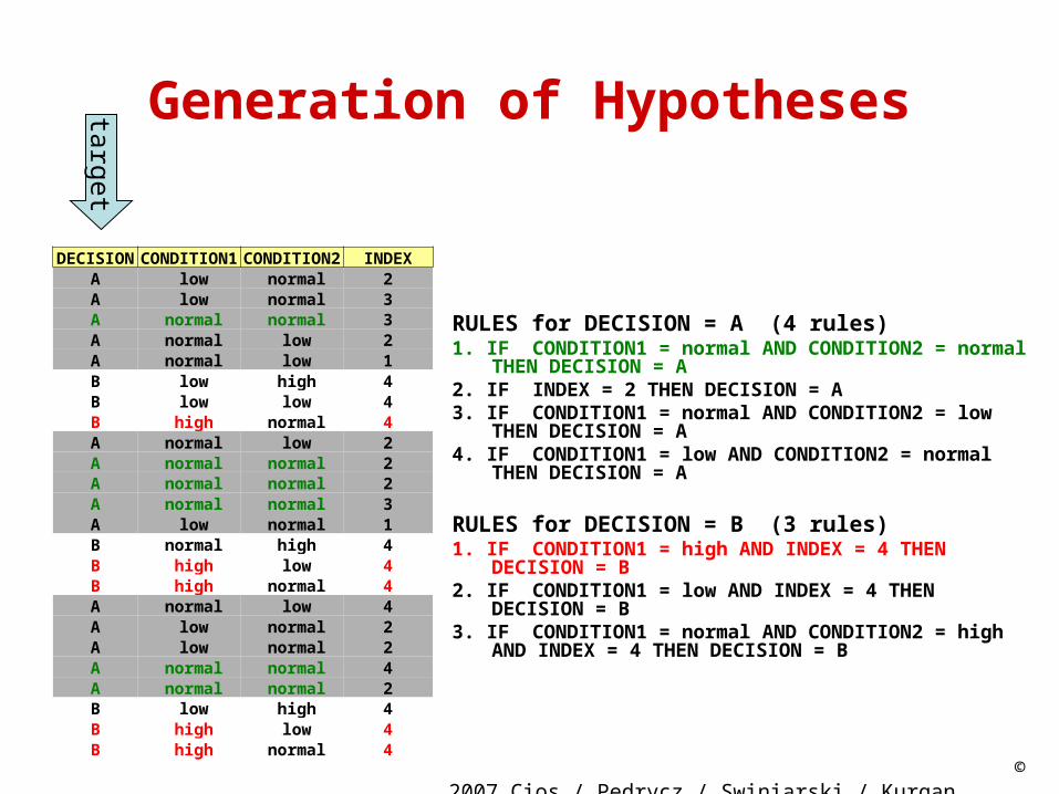
DECISION CONDITION1 CONDITION2 INDEXA low normal 2A low normal 3A normal normal 3A normal low 2A normal low 1B low high 4B low low 4B high normal 4A normal low 2A normal normal 2A normal normal 2A normal normal 3A low normal 1B normal high 4B high low 4B high normal 4A normal low 4A low normal 2A low normal 2A normal normal 4A normal normal 2B low high 4B high low 4B high normal 4
RULES for DECISION = A (4 rules)1. IF CONDITION1 = normal AND CONDITION2 = normal THEN
DECISION = A2. IF INDEX = 2 THEN DECISION = A3. IF CONDITION1 = normal AND CONDITION2 = low THEN
DECISION = A4. IF CONDITION1 = low AND CONDITION2 = normal THEN
DECISION = A
RULES for DECISION = B (3 rules)1. IF CONDITION1 = high AND INDEX = 4 THEN DECISION = B2. IF CONDITION1 = low AND INDEX = 4 THEN DECISION = B3. IF CONDITION1 = normal AND CONDITION2 = high AND
INDEX = 4 THEN DECISION = B
target

© 2007 Cios / Pedrycz / Swiniarski /
Kurgan
Generation of Hypotheses
DECISION CONDITION1 CONDITION2 INDEXA low normal 2A low normal 3A normal normal 3A normal low 2A normal low 1B low high 4B low low 4B high normal 4A normal low 2A normal normal 2A normal normal 2A normal normal 3A low normal 1B normal high 4B high low 4B high normal 4A normal low 4A low normal 2A low normal 2A normal normal 4A normal normal 2B low high 4B high low 4B high normal 4
ASSOCIATION RULES (no “decision” target)
1. DECISION = B AND INDEX = 42. CONDITION1 = normal AND CONDITION2 = normal AND
INDEX = 23. CONDITION2 = normal AND INDEX = 34. DECISION = A AND INDEX = 2etc.

© 2007 Cios / Pedrycz / Swiniarski /
Kurgan
Generation of HypothesesInformation System
IS = < S, Q, V, f >where
S is a finite set of examples S = {e1, ..., ei, ..., eM} M is the number of examples
Q is a finite set of features Q = {F1, ..., Fj, ..., Fn}n is the number of features
is a set of feature values
is the domain of feature
a value of feature
is an information function such that for every and
jFVV
jFV QF j
jFi Vv jF
VQSf
jFii VFef ),( Sei QF j
© 2007 Cios / Pedrycz / Swiniarski /
Kurgan
Generation of Hypotheses
Information System
The set S is often called the learning/training data set.
It is a subset of the entire universe, which is known only to the teacher/oracle,
and is defined as a Cartesian product of all feature domains (j=1,2…n)jF
V
© 2007 Cios / Pedrycz / Swiniarski /
Kurgan
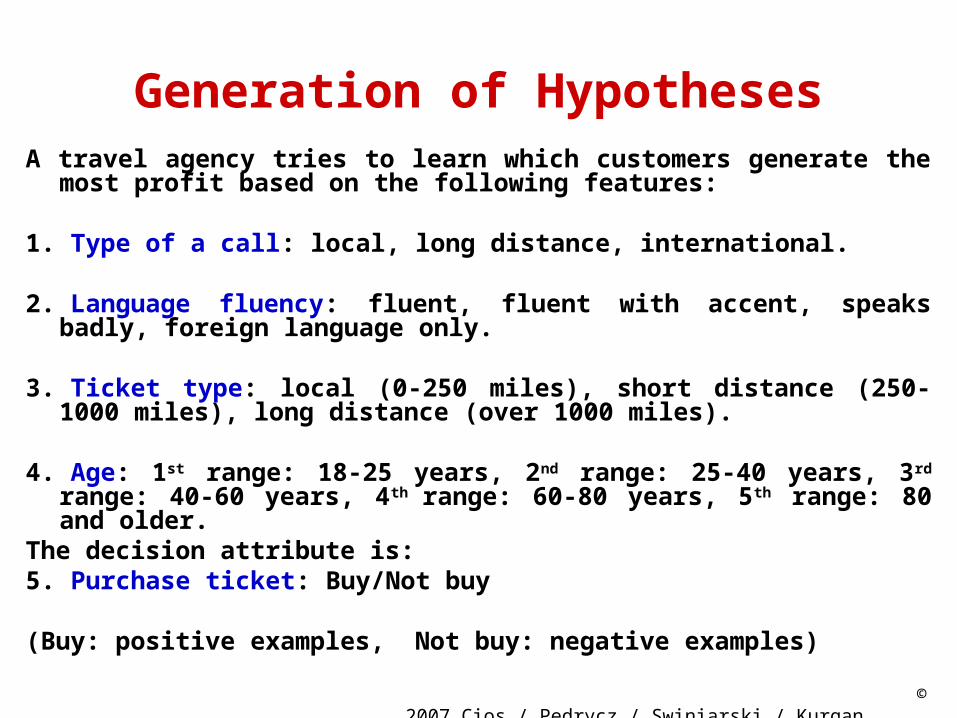
Generation of HypothesesA travel agency tries to learn which customers generate the most profit
based on the following features:
1. Type of a call: local, long distance, international.
2. Language fluency: fluent, fluent with accent, speaks badly, foreign language only.
3. Ticket type: local (0-250 miles), short distance (250-1000 miles), long distance (over 1000 miles).
4. Age: 1st range: 18-25 years, 2nd range: 25-40 years, 3rd range: 40-60 years, 4th range: 60-80 years, 5th range: 80 and older.
The decision attribute is:5. Purchase ticket: Buy/Not buy
(Buy: positive examples, Not buy: negative examples)
© 2007 Cios / Pedrycz / Swiniarski /
Kurgan
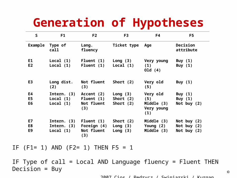
Generation of HypothesesS F1 F2 F3 F4 F5
Example Type of call Lang. fluency Ticket type Age Decision attribute
E1E2
Local (1)Local (1)
Fluent (1)Fluent (1)
Long (3)Local (1)
Very young (1)Old (4)
Buy (1)Buy (1)
E3 Long dist. (2) Not fluent (3) Short (2) Very old (5) Buy (1)
E4E5E6
Intern. (3)Local (1)Local (1)
Accent (2)Fluent (1)Not fluent (3)
Long (3)Short (2)Short (2)
Very old (5)Middle (3)Very young (1)
Buy (1)Buy (1)Not buy (2)
E7E8E9
Intern. (3)Intern. (3)Local (1)
Fluent (1)Foreign (4)Not fluent (3)
Short (2)Long (3)Long (3)
Middle (3)Young (2)Middle (3)
Not buy (2)Not buy (2)Not buy (2)
IF (F1= 1) AND (F2= 1) THEN F5 = 1
IF Type of call = Local AND Language fluency = Fluent THEN Decision = Buy

© 2007 Cios / Pedrycz / Swiniarski /
Kurgan
Generation of Hypotheses
Information System for the example:
S = {e1,…e9}, M = 9
Q = {F1, …F5}, n = 5
VF1= {Local, Long dist., International}
VF2 = {Fluent, Accent, Not fluent, Foreign}
VF3 = {Local, Short, Long}
VF4 = {Very young, Young, Middle, Old, Very old}
VF5 = {Buy, Not buy}

© 2007 Cios / Pedrycz / Swiniarski /
Kurgan
Generation of Hypotheses
It is important to establish a balance between the rules’ generalization and specialization ability
to generate a set of rules that have good predictive power.
A general rule is one that covers many training (positive) examples.
A specialized rule, may cover, in an extreme case, only one example.

© 2007 Cios / Pedrycz / Swiniarski /
Kurgan
Generation of Hypotheses
The rules can be generalized/specialized using the following techniques:
Replace constants with variables: a more general rule is obtained by replacing constants
in rules that have the same IF part, by a variable and thus merging them into one rule
IF F1= krystyna THEN studentIF F1= konrad THEN studentIF F1= karol THEN student can be replaced by a more general rule:IF F1= Soic THEN student

© 2007 Cios / Pedrycz / Swiniarski /
Kurgan
Generation of Hypotheses
Use disjuncts for rule generalization, and conjuncts for rule specialization:
IF F1= 1 AND F2= 5 THEN class1is a more specialized rule (uses conjunct AND) than
IF F1= 1 THEN class1 (OR)IF F2= 5 THEN class1
The last two rules are in implied disjunction, i.e., are connected by a disjunct OR
(any collection of production rules is always OR-ed)

© 2007 Cios / Pedrycz / Swiniarski /
Kurgan
Generation of HypothesesMove up in a hierarchy for generalizationIf there is a known hierarchy the generalization can be done by
replacing the conditions involving the knowledge at the lower level by the common conditions involving the knowledge at the higher level.
IF F1= canary THEN class = sing IF F1= nightingale THEN class = singcan be replaced (if hierarchy of “singbirds” exists) by IF F1= singbird THEN class = sing
ChunkingIs based on the assumption that given the goal every problem
encountered on the way to this goal can be treated as a sub-goal.Then we can generate rules for each of the sub-goals, and put them
together.

© 2007 Cios / Pedrycz / Swiniarski /
Kurgan
Decision Trees
Decision tree consists of nodes and branches connecting the nodes. The nodes located at the bottom of the tree are called leaves, and indicate classes.
The top node in the tree, called the root, contains all training examples that are to be divided into classes.
All nodes, but leaves, in the tree are called decision nodes since they specify a specific decision to be performed at this node based on a single feature.
Each decision node has a number of children nodes, equal to the number of values a given feature assumes.
© 2007 Cios / Pedrycz / Swiniarski /
Kurgan
Decision Trees
© 2007 Cios / Pedrycz / Swiniarski /
Kurgan
Decision Trees
All decision tree algorithms are based on Hunt’s fundamental concept learning algorithm.
It is an embodiment of a method used by humans when learning simple concepts:
it is done by finding key distinguishing features between two categories, represented by the positive and negative (training) examples.
© 2007 Cios / Pedrycz / Swiniarski /
Kurgan
Decision TreesHunt’s algorithm
Given: A set of training examples, S
1. Select the most discriminatory / significant feature
2. Split the entire set, S, located at the root of the tree, into several subsets using the selected feature. The number of children nodes originating from the root is equal to the number of values the selected feature takes on.
3. Recursively find the most significant feature for each subset generated in step 2 and top-down split it into subsets. If each subset (a leaf node) contains examples belonging to one class only then stop, otherwise go to step 3.
Result: The decision tree (from which classification rules can be written out)

© 2007 Cios / Pedrycz / Swiniarski /
Kurgan
Decision Trees
Shannon’s entropy is most often used as a criterion for selecting the most significant/discriminatory feature for splitting the data on:
c
iii ppSEntropy
12 )(log)(
where: pi – probability/proportion of the examples belonging to the ith class
If there were only 2 classes:and the probabilities (pi) were equal (1/2) then Entropy (S) = 1If p1 = 1 (or p2 = 1) then Entropy (S) = 0
In general:0<= Entropy (S) <= log C

© 2007 Cios / Pedrycz / Swiniarski /
Kurgan
Decision Trees
Information Gain measures expected reduction in entropy caused by knowing the value of a feature Fj :
jFi
ii
Vvv
vi SEntropy
S
SSEntropyFSGainnInformatio )()(),(
where
jFV is a set of all possible values of feature jF
ivS is a subset of S, for which feature
jF has value vi.
InfoGain is used to select the best (reducing the entropy by the largest amount) feature at each step of growing a decision tree.

© 2007 Cios / Pedrycz / Swiniarski /
Kurgan
Decision Trees
To eliminate bias in calculating the InfoGain, namely, in a situation when two or more features have the same value of InfoGain the feature that has less number of values is selected, we use a measure called Gain Ratio:
),(
),(),(
j
jj FSnInformatioSplit
FSGainnInformatioFSRatioGain where:
C
i
iij S
S
S
SFSnInformatioSplit
12 )(log),(
Split Information is the entropy of S with respect to values of feature Fj.
Using gain ratio results in generation of smaller trees.

© 2007 Cios / Pedrycz / Swiniarski /
Kurgan
Decision Trees
ID3 algorithmGiven: A set of training examples, S1. Create the root node containing the entire set S2. If all examples are positive (or negative) then stop: decision tree
has one node3. Otherwise (general case)
3.1 Select feature Fj that has the largest Information Gain value3.2 For each value vi from the domain of feature Fj:
a) add a new branch corresponding to this feature value vi and a new node, which stores all the examples that have value vi for feature Fj
b) if the node stores examples belonging to one class only then it becomes a leaf node, else add below this node a new sub-tree, and go to step 3
Result: A decision tree
© 2007 Cios / Pedrycz / Swiniarski /
Kurgan
Decision Trees
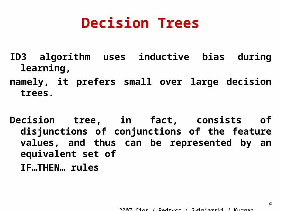
ID3 algorithm uses inductive bias during learning,
namely, it prefers small over large decision trees.
Decision tree, in fact, consists of disjunctions of conjunctions of the feature values, and thus can be represented by an equivalent set of
IF…THEN… rules

© 2007 Cios / Pedrycz / Swiniarski /
Kurgan
Decision TreesOther measures for finding the most discriminatory feature for building decision trees are:
21
( ) ( | ) log ( | )c
i
Entropy n p i n p i n
where p(i│n) denotes fraction of examples from class i at node n.
Instead of entropy we can use misclassification error:
( ) 1 max ( ( | )iMissclassError n p i n
or Gini:2
21
( ) 1 ( | ) log ( | )c
i
Gini n p i n p i n
© 2007 Cios / Pedrycz / Swiniarski /
Kurgan
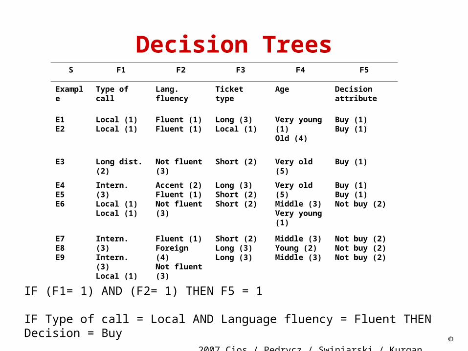
Decision TreesS F1 F2 F3 F4 F5
Example Type of call Lang. fluency Ticket type Age Decision attribute
E1E2
Local (1)Local (1)
Fluent (1)Fluent (1)
Long (3)Local (1)
Very young (1)Old (4)
Buy (1)Buy (1)
E3 Long dist. (2) Not fluent (3) Short (2) Very old (5) Buy (1)
E4E5E6
Intern. (3)Local (1)Local (1)
Accent (2)Fluent (1)Not fluent (3)
Long (3)Short (2)Short (2)
Very old (5)Middle (3)Very young (1)
Buy (1)Buy (1)Not buy (2)
E7E8E9
Intern. (3)Intern. (3)Local (1)
Fluent (1)Foreign (4)Not fluent (3)
Short (2)Long (3)Long (3)
Middle (3)Young (2)Middle (3)
Not buy (2)Not buy (2)Not buy (2)
IF (F1= 1) AND (F2= 1) THEN F5 = 1
IF Type of call = Local AND Language fluency = Fluent THEN Decision = Buy
© 2007 Cios / Pedrycz / Swiniarski /
Kurgan
Decision Trees
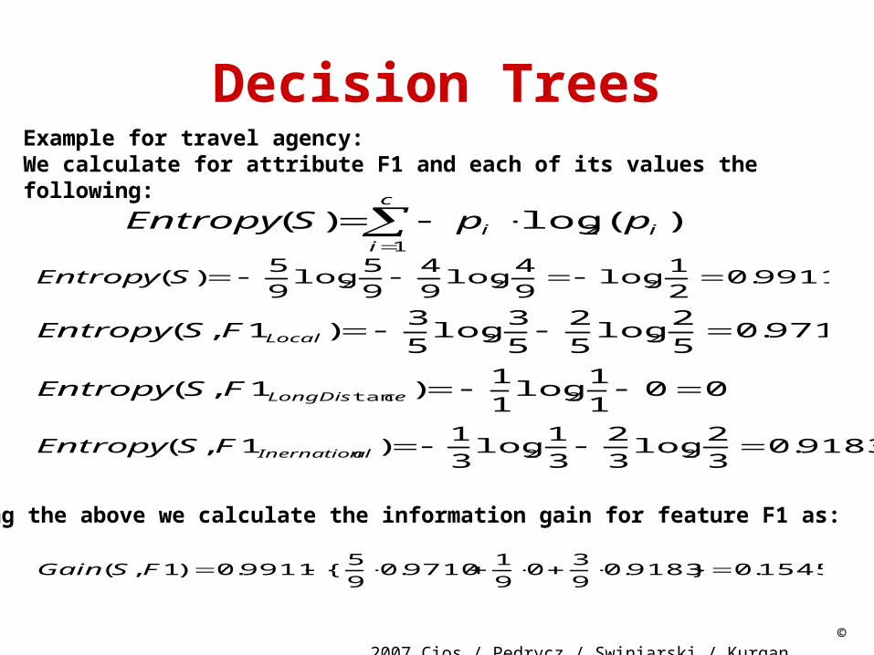
971.05
2log
5
2
5
3log
5
3)1,( 22 LocalFSEntropy
001
1log
1
1)1,( 2tan ceLongDisFSEntropy
9183.03
2log
3
2
3
1log
3
1)1,( 22 alInernationFSEntropy
1545.0}9183.09
30
9
19710.0
9
5{9911.0)1,( FSGain
9911.02
1log
9
4log
9
4
9
5log
9
5)( 222 SEntropy
c
iii ppSEntropy
12 )(log)(
Example for travel agency:We calculate for attribute F1 and each of its values the following:
Having the above we calculate the information gain for feature F1 as:

© 2007 Cios / Pedrycz / Swiniarski /
Kurgan
Decision Trees
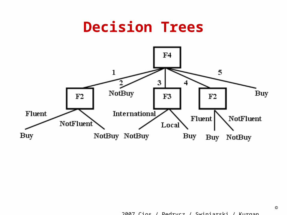
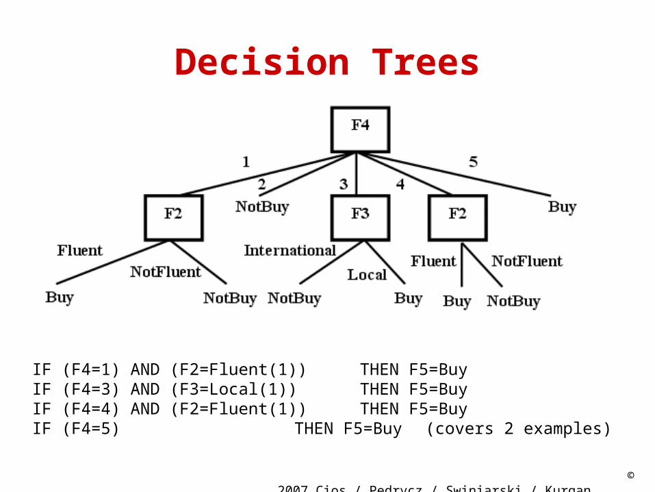
We perform similar calculations for features F2, F3, and F4, and choose the “best” (in terms of the largest value of the information gain) feature.
This feature is F4, and is used at the root of the tree to split the examples into subsets, which are stored at the children nodes.
Next, at each child node we perform the same calculations to find the best feature, at this level of the decision tree, to split the examples on, until the leaf nodes contain examples belonging to one class only
© 2007 Cios / Pedrycz / Swiniarski /
Kurgan
Decision Trees
IF (F4=1) AND (F2=Fluent(1)) THEN F5=BuyIF (F4=3) AND (F3=Local(1)) THEN F5=BuyIF (F4=4) AND (F2=Fluent(1)) THEN F5=BuyIF (F4=5) THEN F5=Buy (covers 2 examples)
© 2007 Cios / Pedrycz / Swiniarski /
Kurgan
Decision Trees
Methods to overcome overfitting in decision tree algorithms:
• Generation of several decision trees instead of one
• Windowing
• Pruning After pruning there should be no significant loss of the classification accuracy; pruning helps to generate more general rules.

© 2007 Cios / Pedrycz / Swiniarski /
Kurgan
Decision Trees
Pruning can be done during the process of tree growing - pre-pruning:
we stop tree-growing when it is determined that no attribute will significantly increase the Gain.
Pruning also can be also done after the entire tree is grown –
post-pruning: some of the branches are removed according to criterion of no significant loss of the rules
accuracy on the training data.
© 2007 Cios / Pedrycz / Swiniarski /
Kurgan
Decision Trees
The extreme case of pre-pruning was introduced by Holte who proposed an algorithm called 1RD for building decision trees that are only one-level deep.
He has shown that the classification performance of such trees is comparable with other more complex algorithms.

© 2007 Cios / Pedrycz / Swiniarski /
Kurgan
Decision TreesWindowing
is a technique to deal with large data
Windowing divides training data into subsets (windows) from which several decision trees are grown.
Then the best rules extracted from these trees are chosen - according to the lowest error-rate on the validation data set.

© 2007 Cios / Pedrycz / Swiniarski /
Kurgan
Decision Trees
C4.5 algorithm is an extension of ID3 that allows for:
• using continuous input values, by using build-in front-end discretization algorithm
• growing trees on data with missing features values

© 2007 Cios / Pedrycz / Swiniarski /
Kurgan
Decision TreesAdvantages and disadvantages of decision trees:
• they reveal relationships between the rules (that can be written out from the tree). Because of this it is easy to see the structure of the data,
• produce rules that best describe all the classes in the training data set,
• are computationally simple,• may generate very complex (long) rules, which are very hard to
prune,• generate large number of corresponding rules. Their number can
become excessively large unless pruning techniques are used to make them more comprehensible,
• require large amounts of memory to store the entire tree for deriving the rules.

© 2007 Cios / Pedrycz / Swiniarski /
Kurgan
Decision Trees
• Decision trees and rule algorithms always create decision boundaries that are parallel to the coordinate axes defined by the features
• In other words, they create hypercube decision regions in high-dimensional spaces
• An obvious remedy for this shortcoming is to have an algorithm that is able to place a decision boundary at any angle. This idea is used in the Continuous ID3 (CID3) neural network algorithm

© 2007 Cios / Pedrycz / Swiniarski /
Kurgan
Decision Trees


![Kedarisetti KD, Mizianty MJ, Dick S, and Kurgan LAbiomine.cs.vcu.edu/papers/posterISMB2009.pdf · Microsoft PowerPoint - Ppt0000007.ppt [Read-Only] Author: Lukasz Kurgan Created Date:](https://img.pdfslide.us/doc/110x75/5fece322269ad6467032ed1f/kedarisetti-kd-mizianty-mj-dick-s-and-kurgan-microsoft-powerpoint-ppt0000007ppt.jpg)