Chapter 1 Algorithms with numbers - Seidenberg School of ...csis.pace.edu/~benjamin/teaching/cs242/webfiles/Book/Chapter1.pdf · Chapter 1 Algorithms with numbers One of the main

P1: OSO/OVY P2: OSO/OVY QC: OSO/OVY T1: OSO

das23402 Ch01 GTBL020-Dasgupta-v10 July 5, 2006 18:4

Chapter 1

Algorithms with numbers

One of the main themes of this chapter is the dramatic contrast between two ancient

problems that at first seem very similar:

FACTORING: Given a number N, express it as a product of its prime factors.

PRIMALITY: Given a number N, determine whether it is a prime.

Factoring is hard. Despite centuries of effort by some of the world’s smartest math-

ematicians and computer scientists, the fastest methods for factoring a number Ntake time exponential in the number of bits of N.

On the other hand, we shall soon see that we can efficiently test whether N is

prime! And (it gets even more interesting) this strange disparity between the two

intimately related problems, one very hard and the other very easy, lies at the heart

of the technology that enables secure communication in today’s global information

environment.

En route to these insights, we need to develop algorithms for a variety of com-

putational tasks involving numbers. We begin with basic arithmetic, an especially

appropriate starting point because, as we know, the word algorithms originally ap-

plied only to methods for these problems.

1.1 Basic arithmetic

1.1.1 Addition

We were so young when we learned the standard technique for addition that we

would scarcely have thought to ask why it works. But let’s go back now and take a

closer look.

It is a basic property of decimal numbers that

The sum of any three single-digit numbers is at most two digits long.

Quick check: the sum is at most 9 + 9 + 9 = 27, two digits long. In fact, this rule

holds not just in decimal but in any base b ≥ 2 (Exercise 1.1). In binary, for instance,

the maximum possible sum of three single-bit numbers is 3, which is a 2-bit number.

11



12 1.1 Basic arithmetic

Bases and logs

Naturally, there is nothing special about the number 10—we just happen to have 10 fingers,and so 10 was an obvious place to pause and take counting to the next level. The Mayansdeveloped a similar positional system based on the number 20 (no shoes, see?). And of coursetoday computers represent numbers in binary.

How many digits are needed to represent the number N ≥ 0 in base b? Let’s see—with kdigits in base b we can express numbers up to bk − 1; for instance, in decimal, three digitsget us all the way up to 999 = 103 − 1. By solving for k, we find that �logb(N + 1)� digits(about logb N digits, give or take 1) are needed to write N in base b.

How much does the size of a number change when we change bases? Recall the rule forconverting logarithms from base a to base b: logb N = (loga N)/(loga b). So the size ofinteger N in base a is the same as its size in base b, times a constant factor loga b. In big-Onotation, therefore, the base is irrelevant, and we write the size simply as O(log N). Whenwe do not specify a base, as we almost never will, we mean log2 N.

Incidentally, this function log N appears repeatedly in our subject, in many guises. Here’s asampling:

1. log N is, of course, the power to which you need to raise 2 in order to obtain N.2. Going backward, it can also be seen as the number of times you must halve N to get

down to 1. (More precisely: �log N�.) This is useful when a number is halved at eachiteration of an algorithm, as in several examples later in the chapter.

3. It is the number of bits in the binary representation of N. (More precisely: �log(N + 1)�.)4. It is also the depth of a complete binary tree with N nodes. (More precisely: �log N�.)

5. It is even the sum 1 + 1

2+ 1

3+ · · · + 1

N, to within a constant factor (Exercise 1.5).

This simple rule gives us a way to add two numbers in any base: align their right-

hand ends, and then perform a single right-to-left pass in which the sum is computed

digit by digit, maintaining the overflow as a carry. Since we know each individual

sum is a two-digit number, the carry is always a single digit, and so at any given

step, three single-digit numbers are added. Here’s an example showing the addition

53 + 35 in binary.

Carry: 1 1 1 1

1 1 0 1 0 1 (53)

1 0 0 0 1 1 (35)

1 0 1 1 0 0 0 (88)

Ordinarily we would spell out the algorithm in pseudocode, but in this case it is so

familiar that we do not repeat it. Instead we move straight to analyzing its efficiency.

Given two binary numbers x and y, how long does our algorithm take to add them?This is the kind of question we shall persistently be asking throughout this book.

We want the answer expressed as a function of the size of the input: the number of

bits of x and y, the number of keystrokes needed to type them in.



Chapter 1 Algorithms 13

Suppose x and y are each n bits long; in this chapter we will consistently use the

letter n for the sizes of numbers. Then the sum of x and y is n + 1 bits at most, and

each individual bit of this sum gets computed in a fixed amount of time. The total

running time for the addition algorithm is therefore of the form c0 + c1n, where c0

and c1 are some constants; in other words, it is linear. Instead of worrying about the

precise values of c0 and c1, we will focus on the big picture and denote the running

time as O(n).

Now that we have a working algorithm whose running time we know, our thoughts

wander inevitably to the question of whether there is something even better.

Is there a faster algorithm? (This is another persistent question.) For addition, the

answer is easy: in order to add two n-bit numbers we must at least read them

and write down the answer, and even that requires n operations. So the addition

algorithm is optimal, up to multiplicative constants!

Some readers may be confused at this point: Why O(n) operations? Isn’t binary

addition something that computers today perform by just one instruction? There

are two answers. First, it is certainly true that in a single instruction we can add

integers whose size in bits is within the word length of today’s computers—32

perhaps. But, as will become apparent later in this chapter, it is often useful and

necessary to handle numbers much larger than this, perhaps several thousand bits

long. Adding and multiplying such large numbers on real computers is very much

like performing the operations bit by bit. Second, when we want to understand

algorithms, it makes sense to study even the basic algorithms that are encoded in

the hardware of today’s computers. In doing so, we shall focus on the bit complexityof the algorithm, the number of elementary operations on individual bits—because

this accounting reflects the amount of hardware, transistors and wires, necessary

for implementing the algorithm.

1.1.2 Multiplication and division

Onward to multiplication! The grade-school algorithm for multiplying two numbers

x and y is to create an array of intermediate sums, each representing the product of

x by a single digit of y. These values are appropriately left-shifted and then added

up. Suppose for instance that we want to multiply 13 × 11, or in binary notation,

x = 1101 and y = 1011. The multiplication would proceed thus.

1 1 0 1

× 1 0 1 1

1 1 0 1 (1101 times 1)

1 1 0 1 (1101 times 1, shifted once)

0 0 0 0 (1101 times 0, shifted twice)

+ 1 1 0 1 (1101 times 1, shifted thrice)

1 0 0 0 1 1 1 1 (binary 143)



14 1.1 Basic arithmetic

In binary this is particularly easy since each intermediate row is either zero or xitself, left-shifted an appropriate amount of times. Also notice that left-shifting is

just a quick way to multiply by the base, which in this case is 2. (Likewise, the

effect of a right shift is to divide by the base, rounding down if needed.)

The correctness of this multiplication procedure is the subject of Exercise 1.6; let’s

move on and figure out how long it takes. If x and y are both n bits, then there are

n intermediate rows, with lengths of up to 2n bits (taking the shifting into account).

The total time taken to add up these rows, doing two numbers at a time, is

O(n) + O(n) + · · · + O(n)︸︷︷︸n − 1 times

,

which is O(n2), quadratic in the size of the inputs: still polynomial but much slower

than addition (as we have all suspected since elementary school).

But Al Khwarizmi knew another way to multiply, a method which is used today in

some European countries. To multiply two decimal numbers x and y, write them

next to each other, as in the example below. Then repeat the following: divide the

first number by 2, rounding down the result (that is, dropping the .5 if the number

was odd), and double the second number. Keep going till the first number gets down

to 1. Then strike out all the rows in which the first number is even, and add up

whatever remains in the second column.

11 13

5 26

2 52 (strike out)

1 104

143 (answer)

But if we now compare the two algorithms, binary multiplication and multiplication

by repeated halvings of the multiplier, we notice that they are doing the same thing!

The three numbers added in the second algorithm are precisely the multiples of 13

by powers of 2 that were added in the binary method. Only this time 11 was not

given to us explicitly in binary, and so we had to extract its binary representation

by looking at the parity of the numbers obtained from it by successive divisions

by 2. Al Khwarizmi’s second algorithm is a fascinating mixture of decimal and

binary!

The same algorithm can thus be repackaged in different ways. For variety we

adopt a third formulation, the recursive algorithm of Figure 1.1, which directly

implements the rule

x · y ={

2(x · �y/2�) if y is even

x + 2(x · �y/2�) if y is odd.

Is this algorithm correct? The preceding recursive rule is transparently correct; so




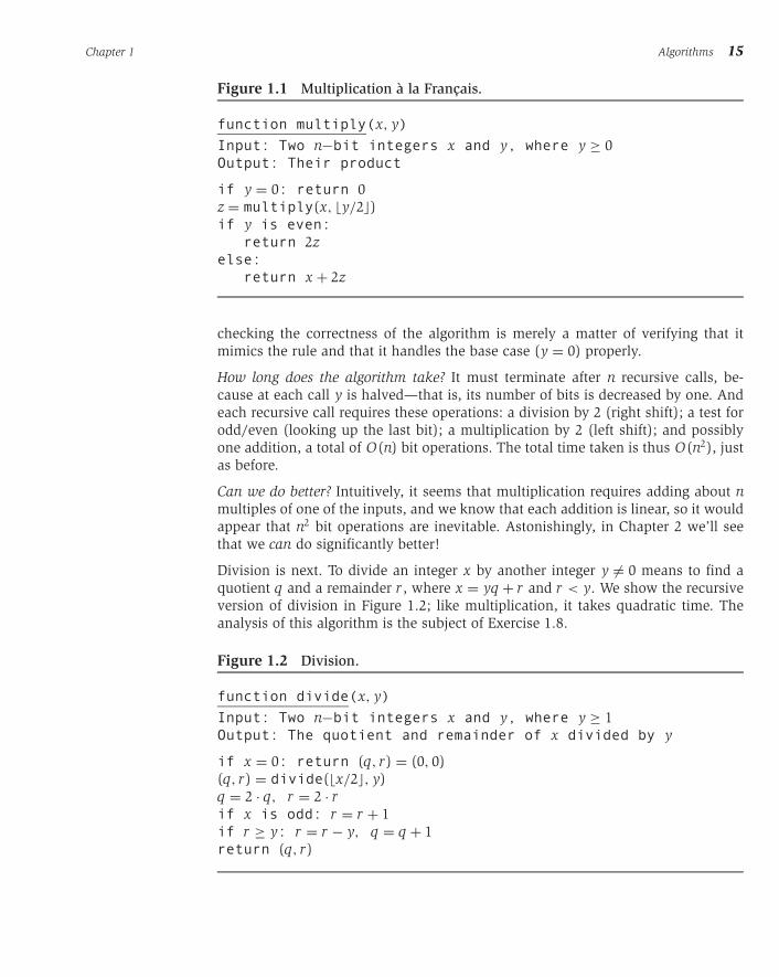
Figure 1.1 Multiplication a la Francais.

function multiply(x, y)

Input: Two n−bit integers x and y, where y ≥ 0

Output: Their product

if y = 0: return 0

z = multiply(x, �y/2�)if y is even:

return 2zelse:

return x + 2z

checking the correctness of the algorithm is merely a matter of verifying that it

mimics the rule and that it handles the base case (y = 0) properly.

How long does the algorithm take? It must terminate after n recursive calls, be-

cause at each call y is halved—that is, its number of bits is decreased by one. And

each recursive call requires these operations: a division by 2 (right shift); a test for

odd/even (looking up the last bit); a multiplication by 2 (left shift); and possibly

one addition, a total of O(n) bit operations. The total time taken is thus O(n2), just

as before.

Can we do better? Intuitively, it seems that multiplication requires adding about nmultiples of one of the inputs, and we know that each addition is linear, so it would

appear that n2 bit operations are inevitable. Astonishingly, in Chapter 2 we’ll see

that we can do significantly better!

Division is next. To divide an integer x by another integer y �= 0 means to find a

quotient q and a remainder r , where x = yq + r and r < y. We show the recursive

version of division in Figure 1.2; like multiplication, it takes quadratic time. The

analysis of this algorithm is the subject of Exercise 1.8.

Figure 1.2 Division.

function divide(x, y)

Input: Two n−bit integers x and y, where y ≥ 1

Output: The quotient and remainder of x divided by y

if x = 0: return (q, r ) = (0, 0)

(q, r ) = divide(�x/2�, y)

q = 2 · q, r = 2 · rif x is odd: r = r + 1

if r ≥ y: r = r − y, q = q + 1

return (q, r )



16 1.2 Modular arithmetic

1.2 Modular arithmeticWith repeated addition or multiplication, numbers can get cumbersomely large. So

it is fortunate that we reset the hour to zero whenever it reaches 24, and the month

to January after every stretch of 12 months. Similarly, for the built-in arithmetic

operations of computer processors, numbers are restricted to some size, 32 bits say,

which is considered generous enough for most purposes.

For the applications we are working toward—primality testing and cryptography—

it is necessary to deal with numbers that are significantly larger than 32 bits, but

whose range is nonetheless limited.

Modular arithmetic is a system for dealing with restricted ranges of integers. We

define x modulo N to be the remainder when x is divided by N; that is, if x = qN + rwith 0 ≤ r < N, then x modulo N is equal to r . This gives an enhanced notion of

equivalence between numbers: x and y are congruent modulo N if they differ by a

multiple of N, or in symbols,

x ≡ y (mod N) ⇐⇒ N divides (x − y).

For instance, 253 ≡ 13 (mod 60) because 253 − 13 is a multiple of 60; more famil-

iarly, 253 minutes is 4 hours and 13 minutes. These numbers can also be negative,

as in 59 ≡ −1 (mod 60): when it is 59 minutes past the hour, it is also 1 minute

short of the next hour.

Figure 1.3 Addition modulo 8.

0 00

+ =6

3

1

One way to think of modular arithmetic is that it limits numbers to a predefined

range {0, 1, . . . , N − 1} and wraps around whenever you try to leave this range—like

the hand of a clock (Figure 1.3).

Another interpretation is that modular arithmetic deals with all the integers, but

divides them into N equivalence classes, each of the form {i + kN : k ∈ Z} for some

i between 0 and N − 1. For example, there are three equivalence classes modulo 3:

· · · −9 −6 −3 0 3 6 9 · · ·· · · −8 −5 −2 1 4 7 10 · · ·· · · −7 −4 −1 2 5 8 11 · · ·

Any member of an equivalence class is substitutable for any other; when viewed

modulo 3, the numbers 5 and 11 are no different. Under such substitutions, addition

and multiplication remain well-defined:




Two’s complement

Modular arithmetic is nicely illustrated in two’s complement, the most common format forstoring signed integers. It uses n bits to represent numbers in the range [−2n−1, 2n−1 − 1]and is usually described as follows:

� Positive integers, in the range 0 to 2n−1 − 1, are stored in regular binary and have aleading bit of 0.

� Negative integers −x , with 1 ≤ x ≤ 2n−1, are stored by first constructing x in binary,then flipping all the bits, and finally adding 1. The leading bit in this case is 1.

(And the usual description of addition and multiplication in this format is even morearcane!)

Here’s a much simpler way to think about it: any number in the range −2n−1 to 2n−1 − 1 isstored modulo 2n . Negative numbers −x therefore end up as 2n − x . Arithmetic operationslike addition and subtraction can be performed directly in this format, ignoring any overflowbits that arise.

Substitution rule If x ≡ x′ (mod N) and y ≡ y′ (mod N), then:

x + y ≡ x′ + y′ (mod N) and xy ≡ x′y′ (mod N).

(See Exercise 1.9.) For instance, suppose you watch an entire season of your favorite

television show in one sitting, starting at midnight. There are 25 episodes, each

lasting 3 hours. At what time of day are you done? Answer: the hour of completion is

(25 × 3) mod 24, which (since 25 ≡ 1 mod 24) is 1 × 3 = 3 mod 24, or three o’clock

in the morning.

It is not hard to check that in modular arithmetic, the usual associative, commu-

tative, and distributive properties of addition and multiplication continue to apply,

for instance:

x + (y + z) ≡ (x + y) + z (mod N) Associativity

xy ≡ yx (mod N) Commutativity

x(y + z) ≡ xy + yz (mod N) Distributivity

Taken together with the substitution rule, this implies that while performing a se-

quence of arithmetic operations, it is legal to reduce intermediate results to their

remainders modulo N at any stage. Such simplifications can be a dramatic help in

big calculations. Witness, for instance:

2345 ≡ (25)69 ≡ 3269 ≡ 169 ≡ 1 (mod 31).

1.2.1 Modular addition and multiplication

To add two numbers x and y modulo N, we start with regular addition. Since x and

y are each in the range 0 to N − 1, their sum is between 0 and 2(N − 1). If the sum




exceeds N − 1, we merely need to subtract off N to bring it back into the required

range. The overall computation therefore consists of an addition, and possibly a

subtraction, of numbers that never exceed 2N. Its running time is linear in the sizes

of these numbers, in other words O(n), where n = �log N� is the size of N; as a

reminder, our convention is to use the letter n to denote input size.

To multiply two mod-N numbers x and y, we again just start with regular multi-

plication and then reduce the answer modulo N. The product can be as large as

(N − 1)2, but this is still at most 2n bits long since log(N − 1)2 = 2 log(N − 1) ≤ 2n.

To reduce the answer modulo N, we compute the remainder upon dividing it by N,

using our quadratic-time division algorithm. Multiplication thus remains a quadratic

operation.

Division is not quite so easy. In ordinary arithmetic there is just one tricky case—

division by zero. It turns out that in modular arithmetic there are potentially other

such cases as well, which we will characterize toward the end of this section.

Whenever division is legal, however, it can be managed in cubic time, O(n3).

To complete the suite of modular arithmetic primitives we need for cryptography, we

next turn to modular exponentiation, and then to the greatest common divisor, which

is the key to division. For both tasks, the most obvious procedures take exponentially

long, but with some ingenuity polynomial-time solutions can be found. A careful

choice of algorithm makes all the difference.

1.2.2 Modular exponentiation

In the cryptosystem we are working toward, it is necessary to compute xy mod N for

values of x, y, and N that are several hundred bits long. Can this be done quickly?

The result is some number modulo N and is therefore itself a few hundred bits long.

However, the raw value of xy could be much, much longer than this. Even when xand y are just 20-bit numbers, xy is at least (219)(219) = 2(19)(524288), about 10 million

bits long! Imagine what happens if y is a 500-bit number!

To make sure the numbers we are dealing with never grow too large, we need

to perform all intermediate computations modulo N. So here’s an idea: calculate

xy mod N by repeatedly multiplying by x modulo N. The resulting sequence of

intermediate products,

x mod N → x2 mod N → x3 mod N → · · · → xy mod N,

consists of numbers that are smaller than N, and so the individual multiplications

do not take too long. But there’s a problem: if y is 500 bits long, we need to perform

y − 1 ≈ 2500 multiplications! This algorithm is clearly exponential in the size of y.

Luckily, we can do better: starting with x and squaring repeatedly modulo N, we

get

x mod N → x2 mod N → x4 mod N → x8 mod N → · · · → x2�log y�mod N.




Each takes just O(log2 N) time to compute, and in this case there are only log ymultiplications. To determine xy mod N, we simply multiply together an appropriate

subset of these powers, those corresponding to 1’s in the binary representation of

y. For instance,

x25 = x110012 = x100002 · x10002 · x12 = x16 · x8 · x1.

A polynomial-time algorithm is finally within reach!

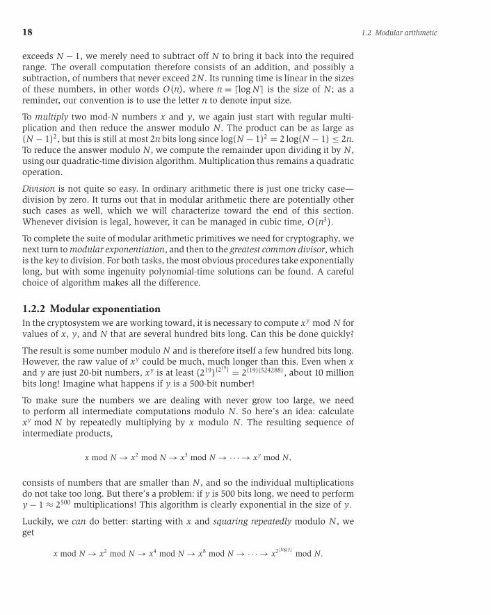
Figure 1.4 Modular exponentiation.

function modexp(x, y, N)

Input: Two n−bit integers x and N, an integer exponent yOutput: xy mod N

if y = 0: return 1

z = modexp(x, �y/2�, N)

if y is even:return z2 mod N

else:return x · z2 mod N

We can package this idea in a particularly simple form: the recursive algorithm of

Figure 1.4, which works by executing, modulo N, the self-evident rule

xy ={ (

x�y/2�)2if y is even

x · (x�y/2�)2

if y is odd.

In doing so, it closely parallels our recursive multiplication algorithm (Figure 1.1).

For instance, that algorithm would compute the product x · 25 by an analogous

decomposition to the one we just saw: x · 25 = x · 16 + x · 8 + x · 1. And whereas

for multiplication the terms x · 2i come from repeated doubling, for exponentiation

the corresponding terms x2i

are generated by repeated squaring.

Let n be the size in bits of x, y, and N (whichever is largest of the three). As with

multiplication, the algorithm will halt after at most n recursive calls, and during

each call it multiplies n-bit numbers (doing computation modulo N saves us here),

for a total running time of O(n3).

1.2.3 Euclid’s algorithm for greatest common divisor

Our next algorithm was discovered well over 2000 years ago by the mathematician

Euclid, in ancient Greece. Given two integers a and b, it finds the largest integer

that divides both of them, known as their greatest common divisor (gcd).

The most obvious approach is to first factor a and b, and then multiply together

their common factors. For instance, 1035 = 32 · 5 · 23 and 759 = 3 · 11 · 23, so their




gcd is 3 · 23 = 69. However, we have no efficient algorithm for factoring. Is there

some other way to compute greatest common divisors?

Euclid’s algorithm uses the following simple formula.

Euclid of Alexandria

BC 325–265

Euclid’s rule If x and y are positive integers with x ≥ y, then gcd(x, y) =gcd(x mod y, y).

Proof. It is enough to show the slightly simpler rule gcd(x, y) = gcd(x − y, y) from

which the one stated can be derived by repeatedly subtracting y from x.

Here it goes. Any integer that divides both x and y must also divide x − y, so

gcd(x, y) ≤ gcd(x − y, y). Likewise, any integer that divides both x − y and y must

also divide both x and y, so gcd(x, y) ≥ gcd(x − y, y).

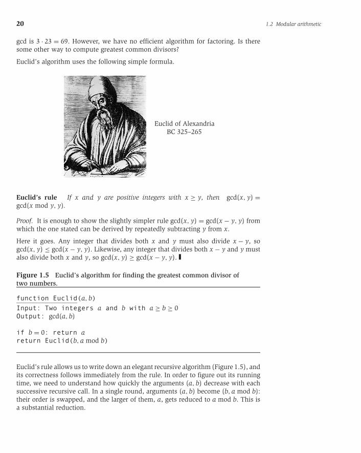
Figure 1.5 Euclid’s algorithm for finding the greatest common divisor oftwo numbers.

function Euclid(a, b)

Input: Two integers a and b with a ≥ b ≥ 0

Output: gcd(a, b)

if b = 0: return areturn Euclid(b, a mod b)

Euclid’s rule allows us to write down an elegant recursive algorithm (Figure 1.5), and

its correctness follows immediately from the rule. In order to figure out its running

time, we need to understand how quickly the arguments (a, b) decrease with each

successive recursive call. In a single round, arguments (a, b) become (b, a mod b):

their order is swapped, and the larger of them, a, gets reduced to a mod b. This is

a substantial reduction.




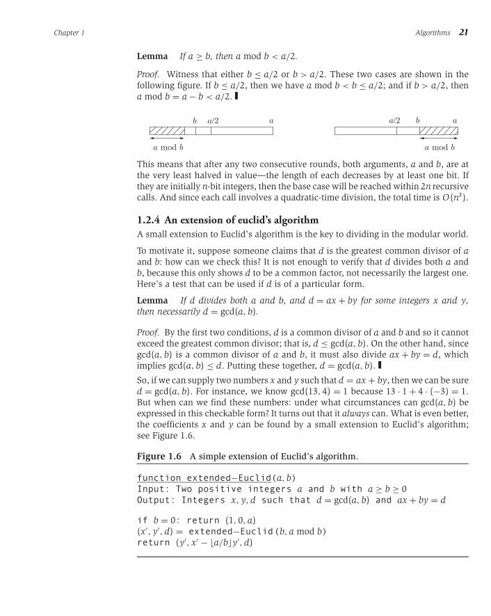
Lemma If a ≥ b, then a mod b < a/2.

Proof. Witness that either b ≤ a/2 or b > a/2. These two cases are shown in the

following figure. If b ≤ a/2, then we have a mod b < b ≤ a/2; and if b > a/2, then

a mod b = a − b < a/2.

a a/2 b a

a mod b

b

a mod b

a/2

This means that after any two consecutive rounds, both arguments, a and b, are at

the very least halved in value—the length of each decreases by at least one bit. If

they are initially n-bit integers, then the base case will be reached within 2n recursive

calls. And since each call involves a quadratic-time division, the total time is O(n3).

1.2.4 An extension of euclid’s algorithm

A small extension to Euclid’s algorithm is the key to dividing in the modular world.

To motivate it, suppose someone claims that d is the greatest common divisor of aand b: how can we check this? It is not enough to verify that d divides both a and

b, because this only shows d to be a common factor, not necessarily the largest one.

Here’s a test that can be used if d is of a particular form.

Lemma If d divides both a and b, and d = ax + by for some integers x and y,then necessarily d = gcd(a, b).

Proof. By the first two conditions, d is a common divisor of a and b and so it cannot

exceed the greatest common divisor; that is, d ≤ gcd(a, b). On the other hand, since

gcd(a, b) is a common divisor of a and b, it must also divide ax + by = d, which

implies gcd(a, b) ≤ d. Putting these together, d = gcd(a, b).

So, if we can supply two numbers x and y such that d = ax + by, then we can be sure

d = gcd(a, b). For instance, we know gcd(13, 4) = 1 because 13 · 1 + 4 · (−3) = 1.

But when can we find these numbers: under what circumstances can gcd(a, b) be

expressed in this checkable form? It turns out that it always can. What is even better,

the coefficients x and y can be found by a small extension to Euclid’s algorithm;

see Figure 1.6.

Figure 1.6 A simple extension of Euclid’s algorithm.

function extended−Euclid(a, b)Input: Two positive integers a and b with a ≥ b ≥ 0

Output: Integers x, y, d such that d = gcd(a, b) and ax + by = d

if b = 0: return (1, 0, a)

(x′, y′, d) = extended−Euclid(b, a mod b)return (y′, x′ − �a/b�y′, d)




Lemma For any positive integers a and b, the extended Euclid algorithm returnsintegers x, y, and d such that gcd(a, b) = d = ax + by.

Proof. The first thing to confirm is that if you ignore the x’s and y’s, the extended

algorithm is exactly the same as the original. So, at least we compute d = gcd(a, b).

For the rest, the recursive nature of the algorithm suggests a proof by induction. The

recursion ends when b = 0, so it is convenient to do induction on the value of b.

The base case b = 0 is easy enough to check directly. Now pick any larger value of

b. The algorithm finds gcd(a, b) by calling gcd(b, a mod b). Since a mod b < b, we

can apply the inductive hypothesis to this recursive call and conclude that the x′

and y′ it returns are correct:

gcd(b, a mod b) = bx′ + (a mod b)y′.

Writing (a mod b) as (a − �a/b�b), we find

d = gcd(a, b) = gcd(b, a mod b) = bx′ + (a mod b)y′

= bx′ + (a − �a/b�b)y′ = ay′ + b(x′ − �a/b�y′).

Therefore d = ax + by with x = y′ and y = x′ − �a/b�y′, thus validating the algo-

rithm’s behavior on input (a, b).

Example. To compute gcd(25, 11), Euclid’s algorithm would proceed as follows:

25 = 2 · 11 + 3

11 = 3 · 3 + 2

3 = 1 · 2 + 1

2 = 2 · 1 + 0

(at each stage, the gcd computation has been reduced to the underlined numbers).

Thus gcd(25, 11) = gcd(11, 3) = gcd(3, 2) = gcd(2, 1) = gcd(1, 0) = 1.

To find x and y such that 25x + 11y = 1, we start by expressing 1 in terms of the

last pair (1, 0). Then we work backwards and express it in terms of (2, 1), (3, 2),

(11, 3), and finally (25, 11). The first step is:

1 = 1 − 0.

To rewrite this in terms of (2, 1), we use the substitution 0 = 2 − 2 · 1 from the last

line of the gcd calculation to get:

1 = 1 − (2 − 2 · 1) = −1 · 2 + 3 · 1.

The second-last line of the gcd calculation tells us that 1 = 3 − 1 · 2. Substituting:

1 = −1 · 2 + 3(3 − 1 · 2) = 3 · 3 − 4 · 2.

Continuing in this same way with substitutions 2 = 11 − 3 · 3 and 3 = 25 − 2 · 11

gives:

1 = 3 · 3 − 4(11 − 3 · 3) = −4 · 11 + 15 · 3 = −4 · 11 + 15(25 − 2 · 11) = 15 · 25 − 34 · 11.

We’re done: 15 · 25 − 34 · 11 = 1, so x = 15 and y = −34.




1.2.5 Modular division

In real arithmetic, every number a �= 0 has an inverse, 1/a, and dividing by a is the

same as multiplying by this inverse. In modular arithmetic, we can make a similar

definition.

We say x is the multiplicative inverse of a modulo N if ax ≡ 1 (mod N).

There can be at most one such x modulo N (Exercise 1.23), and we shall denote it

by a−1. However, this inverse does not always exist! For instance, 2 is not invertible

modulo 6: that is, 2x �≡ 1 mod 6 for every possible choice of x. In this case, a and

N are both even and thus then a mod N is always even, since a mod N = a − kNfor some k. More generally, we can be certain that gcd(a, N) divides ax mod N,

because this latter quantity can be written in the form ax + kN. So if gcd(a, N) > 1,

then ax �≡ 1 mod N, no matter what x might be, and therefore a cannot have a

multiplicative inverse modulo N.

In fact, this is the only circumstance in which a is not invertible. When gcd(a, N) = 1

(we say a and N are relatively prime), the extended Euclid algorithm gives us

integers x and y such that ax + Ny = 1, which means that ax ≡ 1 (mod N). Thus

x is a’s sought inverse.

Example. Continuing with our previous example, suppose we wish to compute

11−1 mod 25. Using the extended Euclid algorithm, we find that 15 · 25 − 34 · 11 = 1.

Reducing both sides modulo 25, we have −34 · 11 ≡ 1 mod 25. So −34 ≡ 16 mod 25

is the inverse of 11 mod 25.

Modular division theorem For any a mod N, a has a multiplicative inverse mod-ulo N if and only if it is relatively prime to N. When this inverse exists, it can befound in time O(n3) (where as usual n denotes the number of bits of N) by runningthe extended Euclid algorithm.

This resolves the issue of modular division: when working modulo N, we can divide

by numbers relatively prime to N—and only by these. And to actually carry out the

division, we multiply by the inverse.

1.3 Primality testingIs there some litmus test that will tell us whether a number is prime without actually

trying to factor the number? We place our hopes in a theorem from the year 1640.

Fermat’s little theorem If p is prime, then for every 1 ≤ a < p,

ap−1 ≡ 1 (mod p).

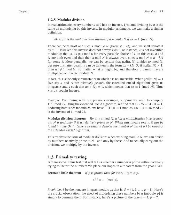
Proof. Let S be the nonzero integers modulo p; that is, S = {1, 2, . . . , p − 1}. Here’s

the crucial observation: the effect of multiplying these numbers by a (modulo p) is

simply to permute them. For instance, here’s a picture of the case a = 3, p = 7:



24 1.3 Primality testing

Is your social security number a prime?

The numbers 7, 17, 19, 71, and 79 are primes, but how about 717-19-7179? Telling whethera reasonably large number is a prime seems tedious because there are far too many candidatefactors to try. However, there are some clever tricks to speed up the process. For instance, youcan omit even-valued candidates after you have eliminated the number 2. You can actuallyomit all candidates except those that are themselves primes.

In fact, a little further thought will convince you that you can proclaim N a prime as soon

as you have rejected all candidates up to√

N, for if N can indeed be factored as N = K · L ,

then it is impossible for both factors to exceed√

N.

We seem to be making progress! Perhaps by omitting more and more candidate factors, atruly efficient primality test can be discovered.

Unfortunately, there is no fast primality test down this road. The reason is that we havebeen trying to tell if a number is a prime by factoring it. And factoring is a hard problem!

Modern cryptography, as well as the balance of this chapter, is about the following importantidea: factoring is hard and primality is easy. We cannot factor large numbers, but we can easilytest huge numbers for primality! (Presumably, if a number is composite, such a test willdetect this without finding a factor.)

6

5

4

3

2

1 1

2

3

4

5

6

Let’s carry this example a bit further. From the picture, we can conclude

{1, 2, . . . , 6} = {3 · 1 mod 7, 3 · 2 mod 7, . . . , 3 · 6 mod 7}.

Multiplying all the numbers in each representation then gives 6! ≡ 36 · 6! (mod 7),

and dividing by 6! we get 36 ≡ 1 (mod 7), exactly the result we wanted in the case

a = 3, p = 7.

Now let’s generalize this argument to other values of a and p, with S= {1, 2, . . . , p − 1}. We’ll prove that when the elements of S are multiplied by amodulo p, the resulting numbers are all distinct and nonzero. And since they lie in

the range [1, p − 1], they must simply be a permutation of S.




The numbers a · i mod p are distinct because if a · i ≡ a · j (mod p), then dividing

both sides by a gives i ≡ j (mod p). They are nonzero because a · i ≡ 0 similarly

implies i ≡ 0. (And we can divide by a, because by assumption it is nonzero and

therefore relatively prime to p.)

We now have two ways to write set S:

S = {1, 2, . . . , p − 1} = {a · 1 mod p, a · 2 mod p, . . . , a · (p − 1) mod p}.

We can multiply together its elements in each of these representations to get

(p − 1)! ≡ ap−1 · (p − 1)! (mod p).

Dividing by (p − 1)! (which we can do because it is relatively prime to p, since pis assumed prime) then gives the theorem.

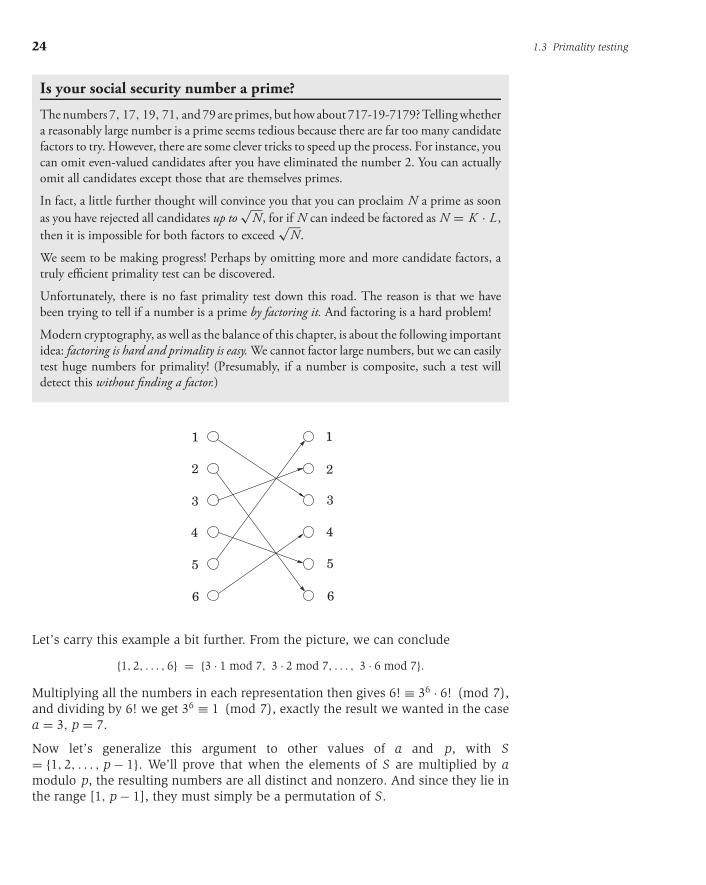
This theorem suggests a “factorless” test for determining whether a number N is

prime:

Is aN−1 ≡ 1 mod N?Pick some a“prime”

“composite”

Fermat’s test

Pass

Fail

The problem is that Fermat’s theorem is not an if-and-only-if condition; it doesn’t

say what happens when N is not prime, so in these cases the preceding diagram is

questionable. In fact, it is possible for a composite number N to pass Fermat’s test

(that is, aN−1 ≡ 1 mod N) for certain choices of a. For instance, 341 = 11 · 31 is not

prime, and yet 2340 ≡ 1 mod 341. Nonetheless, we might hope that for composite N,

most values of a will fail the test. This is indeed true, in a sense we will shortly make

precise, and motivates the algorithm of Figure 1.7: rather than fixing an arbitrary

value of a in advance, we should choose it randomly from {1, . . . , N − 1}.

Figure 1.7 An algorithm for testing primality.

function primality(N)

Input: Positive integer NOutput: yes/no

Pick a positive integer a < N at randomif aN−1 ≡ 1 (mod N):

return yeselse:

return no




Hey, that was group theory!

For any integer N, the set of all numbers mod N that are relatively prime to N constitutewhat mathematicians call a group:

� There is a multiplication operation defined on this set.� The set contains a neutral element (namely 1: any number multiplied by this remains

unchanged).� All elements have a well-defined inverse.

This particular group is called the multiplicative group of N, usually denoted Z∗N .

Group theory is a very well developed branch of mathematics. One of its key concepts is thata group can contain a subgroup—a subset that is a group in and of itself. And an importantfact about a subgroup is that its size must divide the size of the whole group.

Consider now the set B = {b : bN−1 ≡ 1 mod N}. It is not hard to see that it is a subgroupof Z

∗N (just check that B is closed under multiplication and inverses). Thus the size of B

must divide that of Z∗N . Which means that if B doesn’t contain all of Z

∗N , the next largest

size it can have is |Z∗N|/2.

In analyzing the behavior of this algorithm, we first need to get a minor bad case

out of the way. It turns out that certain extremely rare composite numbers N, called

Carmichael numbers, pass Fermat’s test for all a relatively prime to N. On such

numbers our algorithm will fail; but they are pathologically rare, and we will later

see how to deal with them (page 28), so let’s ignore these numbers for the time

being.

In a Carmichael-free universe, our algorithm works well. Any prime number N will

of course pass Fermat’s test and produce the right answer. On the other hand, any

non-Carmichael composite number N must fail Fermat’s test for some value of a;

and as we will now show, this implies immediately that N fails Fermat’s test for atleast half the possible values of a!

Lemma If aN−1 �≡ 1 mod N for some a relatively prime to N, then it must hold forat least half the choices of a < N.

Proof. Fix some value of a for which aN−1 �≡ 1 mod N. The key is to notice that every

element b < N that passes Fermat’s test with respect to N (that is, bN−1 ≡ 1 mod N)

has a twin, a · b, that fails the test:

(a · b)N−1 ≡ aN−1 · bN−1 ≡ aN−1 �≡ 1 mod N.

Moreover, all these elements a · b, for fixed a but different choices of b, are distinct,

for the same reason a · i �≡ a · j in the proof of Fermat’s test: just divide by a.




The one-to-one function b �→ a · b shows that at least as many elements fail the test

as pass it.

FailPass

The set {1, 2, . . . , N−1}

ba · b

We are ignoring Carmichael numbers, so we can now assert

If N is prime, then aN−1 ≡ 1 mod N for all a < N.If N is not prime, then aN−1 ≡ 1 mod N for at most half the values of a < N.

The algorithm of Figure 1.7 therefore has the following probabilistic behavior.

Pr(Algorithm 1.7 returns yes when N is prime) = 1

Pr(Algorithm 1.7 returns yes when N is not prime) ≤ 1

2

We can reduce this one-sided error by repeating the procedure many times, by ran-

domly picking several values of a and testing them all (Figure 1.8).

Pr(Algorithm 1.8 returns yes when N is not prime) ≤ 1

2k

This probability of error drops exponentially fast, and can be driven arbitrarily low

by choosing k large enough. Testing k = 100 values of a makes the probability of

failure at most 2−100, which is miniscule: far less, for instance, than the probability

that a random cosmic ray will sabotage the computer during the computation!

Figure 1.8 An algorithm for testing primality, with low error probability.

function primality2(N)

Input: Positive integer NOutput: yes/no

Pick positive integers a1, a2, . . . , ak < N at randomif aN−1

i ≡ 1 (mod N) for all i = 1, 2, . . . , k:

return yeselse:

return no




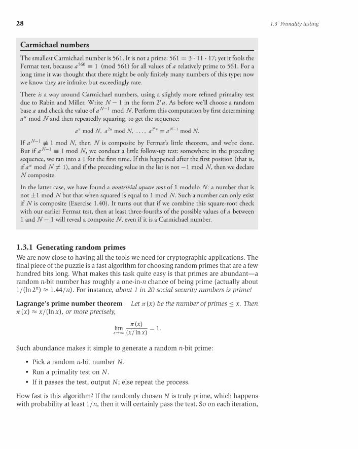
Carmichael numbers

The smallest Carmichael number is 561. It is not a prime: 561 = 3 · 11 · 17; yet it fools theFermat test, because a560 ≡ 1 (mod 561) for all values of a relatively prime to 561. For along time it was thought that there might be only finitely many numbers of this type; nowwe know they are infinite, but exceedingly rare.

There is a way around Carmichael numbers, using a slightly more refined primality testdue to Rabin and Miller. Write N − 1 in the form 2t u. As before we’ll choose a randombase a and check the value of a N−1 mod N. Perform this computation by first determiningau mod N and then repeatedly squaring, to get the sequence:

au mod N, a 2u mod N, . . . , a 2t u = a N−1 mod N.

If a N−1 �≡ 1 mod N, then N is composite by Fermat’s little theorem, and we’re done.But if a N−1 ≡ 1 mod N, we conduct a little follow-up test: somewhere in the precedingsequence, we ran into a 1 for the first time. If this happened after the first position (that is,if au mod N �= 1), and if the preceding value in the list is not −1 mod N, then we declareN composite.

In the latter case, we have found a nontrivial square root of 1 modulo N: a number that isnot ±1 mod N but that when squared is equal to 1 mod N. Such a number can only existif N is composite (Exercise 1.40). It turns out that if we combine this square-root checkwith our earlier Fermat test, then at least three-fourths of the possible values of a between1 and N − 1 will reveal a composite N, even if it is a Carmichael number.

1.3.1 Generating random primes

We are now close to having all the tools we need for cryptographic applications. The

final piece of the puzzle is a fast algorithm for choosing random primes that are a few

hundred bits long. What makes this task quite easy is that primes are abundant—a

random n-bit number has roughly a one-in-n chance of being prime (actually about

1/(ln 2n) ≈ 1.44/n). For instance, about 1 in 20 social security numbers is prime!

Lagrange’s prime number theorem Let π(x) be the number of primes ≤ x. Thenπ(x) ≈ x/(ln x), or more precisely,

limx→∞

π(x)

(x/ ln x)= 1.

Such abundance makes it simple to generate a random n-bit prime:

� Pick a random n-bit number N.� Run a primality test on N.� If it passes the test, output N; else repeat the process.

How fast is this algorithm? If the randomly chosen N is truly prime, which happens

with probability at least 1/n, then it will certainly pass the test. So on each iteration,




Randomized algorithms: a virtual chapter

Surprisingly—almost paradoxically—some of the fastest and most clever algorithms we haverely on chance: at specified steps they proceed according to the outcomes of random cointosses. These randomized algorithms are often very simple and elegant, and their output iscorrect with high probability. This success probability does not depend on the randomnessof the input; it only depends on the random choices made by the algorithm itself.

Instead of devoting a special chapter to this topic, in this book we intersperse randomizedalgorithms at the chapters and sections where they arise most naturally. Furthermore, nospecialized knowledge of probability is necessary to follow what is happening. You justneed to be familiar with the concept of probability, expected value, the expected numberof times we must flip a coin before getting heads, and the property known as “linearity ofexpectation.”

Here are pointers to the major randomized algorithms in this book: One of the earliestand most dramatic examples of a randomized algorithm is the randomized primality test ofFigure 1.8. Hashing is a general randomized data structure that supports inserts, deletes, andlookups and is described later in this chapter, in Section 1.5. Randomized algorithms forsorting and median finding are described in Chapter 2. A randomized algorithm for the mincut problem is described in the box on page 139. Randomization plays an important rolein heuristics as well; these are described in Section 9.3. And finally the quantum algorithmfor factoring (Section 10.7) works very much like a randomized algorithm, its output beingcorrect with high probability—except that it draws its randomness not from coin tosses, butfrom the superposition principle in quantum mechanics.

this procedure has at least a 1/n chance of halting. Therefore on average it will halt

within O(n) rounds (Exercise 1.34).

Next, exactly which primality test should be used? In this application, since the

numbers we are testing for primality are chosen at random rather than by an ad-

versary, it is sufficient to perform the Fermat test with base a = 2 (or to be really

safe, a = 2, 3, 5), because for random numbers the Fermat test has a much smaller

failure probability than the worst-case 1/2 bound that we proved earlier. Numbers

that pass this test have been jokingly referred to as “industrial grade primes.” The

resulting algorithm is quite fast, generating primes that are hundreds of bits long in

a fraction of a second on a PC.

The important question that remains is: what is the probability that the output of the

algorithm is really prime? To answer this we must first understand how discerning

the Fermat test is. As a concrete example, suppose we perform the test with base a= 2 for all numbers N ≤ 25 × 109. In this range, there are about 109 primes, and

about 20,000 composites that pass the test (see the following figure). Thus the

chance of erroneously outputting a composite is approximately 20,000/109 = 2 ×10−5. This chance of error decreases rapidly as the length of the numbers involved

is increased (to the few hundred digits we expect in our applications).



30 1.4 Cryptography

Fermat test(base a = 2)

Composites

Pass

Fail

≈ 109 primes

≈ 20,000 composites

Before primality test:all numbers After primality test

Primes

≤ 25×109

1.4 CryptographyOur next topic, the Rivest-Shamir-Adelman (RSA) cryptosystem, uses all the ideas

we have introduced in this chapter! It derives very strong guarantees of security by

ingeniously exploiting the wide gulf between the polynomial-time computability of

certain number-theoretic tasks (modular exponentiation, greatest common divisor,

primality testing) and the intractability of others (factoring).

The typical setting for cryptography can be described via a cast of three characters:

Alice and Bob, who wish to communicate in private, and Eve, an eavesdropper

who will go to great lengths to find out what they are saying. For concreteness,

let’s say Alice wants to send a specific message x, written in binary (why not),

to her friend Bob. She encodes it as e(x), sends it over, and then Bob applies his

decryption function d(·) to decode it: d(e(x)) = x. Here e(·) and d(·) are appropriate

transformations of the messages.

Eve

BobAlice

Encoder Decoderx x = d(e(x))e(x)

Alice and Bob are worried that the eavesdropper, Eve, will intercept e(x): for in-

stance, she might be a sniffer on the network. But ideally the encryption function

e(·) is so chosen that without knowing d(·), Eve cannot do anything with the infor-

mation she has picked up. In other words, knowing e(x) tells her little or nothing

about what x might be.

For centuries, cryptography was based on what we now call private-key protocols.In such a scheme, Alice and Bob meet beforehand and together choose a secret

codebook, with which they encrypt all future correspondence between them. Eve’s

only hope, then, is to collect some encoded messages and use them to at least

partially figure out the codebook.




An application of number theory?

The renowned mathematician G. H. Hardy once declared of his work: “I have never doneanything useful.” Hardy was an expert in the theory of numbers, which has long beenregarded as one of the purest areas of mathematics, untarnished by material motivationand consequence. Yet the work of thousands of number theorists over the centuries, Hardy’sincluded, is now crucial to the operation of Web browsers and cell phones and to the securityof financial transactions worldwide.

Public-key schemes such as RSA are significantly more subtle and tricky: they allow

Alice to send Bob a message without ever having met him before. This almost sounds

impossible, because in this scenario there is a symmetry between Bob and Eve: why

should Bob have any advantage over Eve in terms of being able to understand Alice’s

message? The central idea behind the RSA cryptosystem is that using the dramatic

contrast between factoring and primality, Bob is able to implement a digital lock, to

which only he has the key. Now by making this digital lock public, he gives Alice

a way to send him a secure message, which only he can open. Moreover, this is

exactly the scenario that comes up in Internet commerce, for example, when you

wish to send your credit card number to some company over the Internet.

In the RSA protocol, Bob need only perform the simplest of calculations, such as

multiplication, to implement his digital lock. Similarly Alice and Bob need only per-

form simple calculations to lock and unlock the message respectively—operations

that any pocket computing device could handle. By contrast, to unlock the message

without the key, Eve must perform operations like factoring large numbers, which

requires more computational power than would be afforded by the world’s most

powerful computers combined. This compelling guarantee of security explains why

the RSA cryptosystem is such a revolutionary development in cryptography.

1.4.1 Private-key schemes: one-time pad and AES

If Alice wants to transmit an important private message to Bob, it would be wise of

her to scramble it with an encryption function,

e : 〈messages〉 → 〈encoded messages〉.

Of course, this function must be invertible—for decoding to be possible—and is

therefore a bijection. Its inverse is the decryption function d(·).In the one-time pad, Alice and Bob meet beforehand and secretly choose a bi-

nary string r of the same length—say, n bits—as the important message x that

Alice will later send. Alice’s encryption function is then a bitwise exclusive-or, er (x)

= x ⊕ r : each position in the encoded message is the exclusive-or of the correspond-

ing positions in x and r . For instance, if r = 01110010, then the message 11110000 is

scrambled thus:

er (11110000) = 11110000 ⊕ 01110010 = 10000010.



32 1.4 Cryptography

This function er is a bijection from n-bit strings to n-bit strings, as evidenced by the

fact that it is its own inverse!

er (er (x)) = (x ⊕ r ) ⊕ r = x ⊕ (r ⊕ r ) = x ⊕ 0 = x,

where 0 is the string of all zeros. Thus Bob can decode Alice’s transmission by

applying the same encryption function a second time: dr (y) = y ⊕ r .

How should Alice and Bob choose r for this scheme to be secure? Simple: they should

pick r at random, flipping a coin for each bit, so that the resulting string is equally

likely to be any element of {0, 1}n. This will ensure that if Eve intercepts the encoded

message y = er (x), she gets no information about x. Suppose, for example, that Eve

finds out y = 10; what can she deduce? She doesn’t know r , and the possible values

it can take all correspond to different original messages x:

00

01

10

11

x

10

e11

e01

e00

y

e10

So given what Eve knows, all possibilities for x are equally likely!

The downside of the one-time pad is that it has to be discarded after use, hence the

name. A second message encoded with the same pad would not be secure, because

if Eve knew x ⊕ r and z ⊕ r for two messages x and z, then she could take the

exclusive-or to get x ⊕ z, which might be important information—for example, (1)

it reveals whether the two messages begin or end the same, and (2) if one message

contains a long sequence of zeros (as could easily be the case if the message is an

image), then the corresponding part of the other message will be exposed. Therefore

the random string that Alice and Bob share has to be the combined length of all the

messages they will need to exchange.

The one-time pad is a toy cryptographic scheme whose behavior and theoretical

properties are completely clear. At the other end of the spectrum lies the advancedencryption standard (AES), a very widely used cryptographic protocol that was

approved by the U.S. National Institute of Standards and Technologies in 2001. AES

is once again private-key: Alice and Bob have to agree on a shared random string

r . But this time the string is of a small fixed size, 128 to be precise (variants with

192 or 256 bits also exist), and specifies a bijection er from 128-bit strings to 128-bit

strings. The crucial difference is that this function can be used repeatedly, so for

instance a long message can be encoded by splitting it into segments of 128 bits

and applying er to each segment.




The security of AES has not been rigorously established, but certainly at present

the general public does not know how to break the code—to recover x from er (x)—

except using techniques that are not very much better than the brute-force approach

of trying all possibilities for the shared string r .

1.4.2 RSA

Unlike the previous two protocols, the RSA scheme is an example of public-keycryptography: anybody can send a message to anybody else using publicly available

information, rather like addresses or phone numbers. Each person has a public

key known to the whole world and a secret key known only to him- or herself.

When Alice wants to send message x to Bob, she encodes it using his public key.

He decrypts it using his secret key, to retrieve x. Eve is welcome to see as many

encrypted messages for Bob as she likes, but she will not be able to decode them,

under certain simple assumptions.

The RSA scheme is based heavily upon number theory. Think of messages from Alice

to Bob as numbers modulo N; messages larger than N can be broken into smaller

pieces. The encryption function will then be a bijection on {0, 1, . . . , N − 1}, and

the decryption function will be its inverse. What values of N are appropriate, and

what bijection should be used?

Property Pick any two primes p and q and let N = pq. For any e relatively primeto (p − 1)(q − 1):

1. The mapping x �→ xe mod N is a bijection on {0, 1, . . . , N − 1}.2. Moreover, the inverse mapping is easily realized: let d be the inverse of e modulo

(p − 1)(q − 1). Then for all x ∈ {0, . . . , N − 1},

(xe)d ≡ x mod N.

The first property tells us that the mapping x �→ xe mod N is a reasonable way to

encode messages x; no information is lost. So, if Bob publishes (N, e) as his publickey, everyone else can use it to send him encrypted messages. The second property

then tells us how decryption can be achieved. Bob should retain the value d as

his secret key, with which he can decode all messages that come to him by simply

raising them to the dth power modulo N.

Example. Let N = 55 = 5 · 11. Choose encryption exponent e = 3, which satisfies

the condition gcd(e, (p − 1)(q − 1)) = gcd(3, 40) = 1. The decryption exponent is

then d = 3−1 mod 40 = 27. Now for any message x mod 55, the encryption of xis y = x3 mod 55, and the decryption of y is x = y27 mod 55. So, for example, if

x = 13, then y = 133 = 52 mod 55 and 13 = 5227 mod 55.

Let’s prove the assertion above and then examine the security of the scheme.



34 1.4 Cryptography

Proof. If the mapping x �→ xe mod N is invertible, it must be a bijection; hence

statement 2 implies statement 1. To prove statement 2, we start by observing that e is

invertible modulo (p − 1)(q − 1) because it is relatively prime to this number. To see

that (xe)d ≡ x mod N, we examine the exponent: since ed ≡ 1 mod (p − 1)(q − 1),

we can write ed in the form 1 + k(p − 1)(q − 1) for some k. Now we need to show

that the difference

xed − x = x1+k(p−1)(q−1) − x

is always 0 modulo N. The second form of the expression is convenient because

it can be simplified using Fermat’s little theorem. It is divisible by p (since xp−1

≡ 1 mod p) and likewise by q. Since p and q are primes, this expression must also

be divisible by their product N. Hence xed − x = x1+k(p−1)(q−1) − x ≡ 0 (mod N),

exactly as we need.

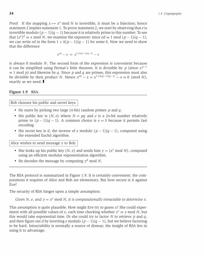
Figure 1.9 RSA.

Bob chooses his public and secret keys.

� He starts by picking two large (n-bit) random primes p and q.� His public key is (N, e) where N = pq and e is a 2n-bit number relatively

prime to (p − 1)(q − 1). A common choice is e = 3 because it permits fast

encoding.� His secret key is d, the inverse of e modulo (p − 1)(q − 1), computed using

the extended Euclid algorithm.

Alice wishes to send message x to Bob.

� She looks up his public key (N, e) and sends him y = (xe mod N), computed

using an efficient modular exponentiation algorithm.� He decodes the message by computing yd mod N.

The RSA protocol is summarized in Figure 1.9. It is certainly convenient: the com-

putations it requires of Alice and Bob are elementary. But how secure is it against

Eve?

The security of RSA hinges upon a simple assumption:

Given N, e, and y = xe mod N, it is computationally intractable to determine x.

This assumption is quite plausible. How might Eve try to guess x? She could exper-

iment with all possible values of x, each time checking whether xe ≡ y mod N, but

this would take exponential time. Or she could try to factor N to retrieve p and q,

and then figure out d by inverting e modulo (p − 1)(q − 1), but we believe factoring

to be hard. Intractability is normally a source of dismay; the insight of RSA lies in

using it to advantage.




1.5 Universal hashingWe end this chapter with an application of number theory to the design of hashfunctions. Hashing is a very useful method of storing data items in a table so as to

support insertions, deletions, and lookups.

Suppose, for instance, that we need to maintain an ever-changing list of about

250 IP (Internet protocol) addresses, perhaps the addresses of the currently active

customers of a Web service. (Recall that an IP address consists of 32 bits encoding

the location of a computer on the Internet, usually shown broken down into four

8-bit fields, for example, 128.32.168.80.) We could obtain fast lookup times if we

maintained the records in an array indexed by IP address. But this would be very

wasteful of memory: the array would have 232 ≈ 4 × 109 entries, the vast majority

of them blank. Or alternatively, we could use a linked list of just the 250 records.

But then accessing records would be very slow, taking time proportional to 250, the

total number of customers. Is there a way to get the best of both worlds, to use an

amount of memory that is proportional to the number of customers and yet also

achieve fast lookup times? This is exactly where hashing comes in.

1.5.1 Hash tables

Here’s a high-level view of hashing. We will give a short “nickname” to each of the

232 possible IP addresses. You can think of this short name as just a number between

1 and 250 (we will later adjust this range very slightly). Thus many IP addresses

will inevitably have the same nickname; however, we hope that most of the 250 IP

addresses of our particular customers are assigned distinct names, and we will store

their records in an array of size 250 indexed by these names. What if there is more

than one record associated with the same name? Easy: each entry of the array points

to a linked list containing all records with that name. So the total amount of storage

is proportional to 250, the number of customers, and is independent of the total

number of possible IP addresses. Moreover, if not too many customer IP addresses

are assigned the same name, lookup is fast, because the average size of the linked

list we have to scan through is small.

But how do we assign a short name to each IP address? This is the role of a hashfunction: in our example, a function h that maps IP addresses to positions in a table

of length about 250 (the expected number of data items). The name assigned to an

x

y

z

x y

z

Space of all 232 IP addresses

250 IPs

Hash table

h

of size ≈ 250



36 1.5 Universal hashing

IP address x is thus h(x), and the record for x is stored in position h(x) of the table.

As described before, each position of the table is in fact a bucket, a linked list that

contains all current IP addresses that map to it. Hopefully, there will be very few

buckets that contain more than a handful of IP addresses.

1.5.2 Families of hash functions

Designing hash functions is tricky. A hash function must in some sense be “ran-

dom” (so that it scatters data items around), but it should also be a function and

therefore “consistent” (so that we get the same result every time we apply it). And

the statistics of the data items may work against us. In our example, one possi-

ble hash function would map an IP address to the 8-bit number that is its last

segment: h(128.32.168.80) = 80. A table of n = 256 buckets would then be required.

But is this a good hash function? Not if, for example, the last segment of an IP

address tends to be a small (single- or double-digit) number; then low-numbered

buckets would be crowded. Taking the first segment of the IP address also invites

disaster—for example, if most of our customers come from Asia.

There is nothing inherently wrong with these two functions. If our 250 IP addresses

were uniformly drawn from among all N = 232 possibilities, then these functions

would behave well. The problem is we have no guarantee that the distribution of

IP addresses is uniform.

Conversely, there is no single hash function, no matter how sophisticated, that

behaves well on all sets of data. Since a hash function maps 232 IP addresses to

just 250 names, there must be a collection of at least 232/250 ≈ 224 ≈ 16,000,000 IP

addresses that are assigned the same name (or, in hashing terminology, “collide”).

If many of these show up in our customer set, we’re in trouble.

Obviously, we need some kind of randomization. Here’s an idea: let us pick a

hash function at random from some class of functions. We will then show that, no

matter what set of 250 IP addresses we actually care about, most choices of the

hash function will give very few collisions among these addresses.

To this end, we need to define a class of hash functions from which we can pick

at random; and this is where we turn to number theory. Let us take the number

of buckets to be not 250 but n = 257—a prime number! And we consider every IP

address x as a quadruple x = (x1, . . . , x4) of integers modulo n—recall that it is in

fact a quadruple of integers between 0 and 255, so there is no harm in this. We can

define a function h from IP addresses to a number mod n as follows: fix any four

numbers mod n = 257, say 87, 23, 125, and 4. Now map the IP address (x1, . . . , x4)

to h(x1, . . . , x4) = (87x1 + 23x2 + 125x3 + 4x4) mod 257. Indeed, any four numbers

mod n define a hash function.

For any four coefficients a1, . . . , a4 ∈ {0, 1, . . . , n − 1}, write a = (a1, a2, a3, a4) and

define ha to be the following hash function:

ha(x1, . . . , x4) =4∑

i=1

ai · xi mod n.




We will show that if we pick these coefficients a at random, then ha is very likely

to be good in the following sense.

Property Consider any pair of distinct IP addresses x = (x1, . . . , x4) and y= (y1, . . . , y4). If the coefficients a = (a1, a2, a3, a4) are chosen uniformly at randomfrom {0, 1, . . . , n − 1}, then

Pr {ha(x1, . . . , x4) = ha(y1, . . . , y4)} = 1

n.

In other words, the chance that x and y collide under ha is the same as it would

be if each were assigned nicknames randomly and independently. This condition

guarantees that the expected lookup time for any item is small. Here’s why. If we

wish to look up x in our hash table, the time required is dominated by the size of

its bucket, that is, the number of items that are assigned the same name as x. But

there are only 250 items in the hash table, and the probability that any one item

gets the same name as x is 1/n = 1/257. Therefore the expected number of items

that are assigned the same name as x by a randomly chosen hash function ha is

250/257 ≈ 1, which means the expected size of x’s bucket is less than 2.1

Let us now prove the preceding property.

Proof. Since x = (x1, . . . , x4) and y = (y1, . . . , y4) are distinct, these quadruples

must differ in some component; without loss of generality let us assume that x4 �= y4.

We wish to compute the probability Pr[ha(x1, . . . , x4) = ha(y1, . . . , y4)], that is, the

probability that∑4

i=1 ai · xi ≡ ∑4i=1 ai · yi mod n. This last equation can be rewritten

as

3∑i=1

ai · (xi − yi) ≡ a4 · (y4 − x4) mod n. (1)

Suppose that we draw a random hash function ha by picking a = (a1, a2, a3, a4) at

random. We start by drawing a1, a2, and a3, and then we pause and think: What

is the probability that the last drawn number a4 is such that equation (1) holds? So

far the left-hand side of equation (1) evaluates to some number, call it c. And since

n is prime and x4 �= y4, (y4 − x4) has a unique inverse modulo n. Thus for equation

(1) to hold, the last number a4 must be precisely c · (y4 − x4)−1 mod n, out of its n

possible values. The probability of this happening is 1/n, and the proof is complete.

Let us step back and see what we just achieved. Since we have no control over

the set of data items, we decided instead to select a hash function h uniformly at

1When a hash function ha is chosen at random, let the random variable Yi (for i = 1, . . . , 250) be 1 if

item i gets the same name as x and 0 otherwise. So the expected value of Yi is 1/n. Now,

Y = Y1 + Y2 + · · · + Y250 is the number of items which get the same name as x, and by linearity of

expectation, the expected value of Y is simply the sum of the expected values of Y1 through Y250. It is

thus 250/n = 250/257.



38 Exercises

random from among a family H of hash functions. In our example,

H = {ha : a ∈ {0, . . . , n − 1}4}.

To draw a hash function uniformly at random from this family, we just draw four

numbers a1, . . . , a4 modulo n. (Incidentally, notice that the two simple hash func-

tions we considered earlier, namely, taking the last or the first 8-bit segment, belong

to this class. They are h(0,0,0,1) and h(1,0,0,0), respectively.) And we insisted that the

family have the following property:

For any two distinct data items x and y, exactly |H|/n of all the hash functionsin H map x and y to the same bucket, where n is the number of buckets.

A family of hash functions with this property is called universal. In other words, for

any two data items, the probability these items collide is 1/n if the hash function

is randomly drawn from a universal family. This is also the collision probability if

we map x and y to buckets uniformly at random—in some sense the gold standard

of hashing. We then showed that this property implies that hash table operations

have good performance in expectation.

This idea, motivated as it was by the hypothetical IP address application, can of

course be applied more generally. Start by choosing the table size n to be some

prime number that is a little larger than the number of items expected in the table

(there is usually a prime number close to any number we start with; actually, to

ensure that hash table operations have good performance, it is better to have the

size of the hash table be about twice as large as the number of items). Next assume

that the size of the domain of all data items is N = nk, a power of n (if we need to

overestimate the true number of data items, so be it). Then each data item can be

considered as a k-tuple of integers modulo n, and H = {ha : a ∈ {0, . . . , n − 1}k} is

a universal family of hash functions.

Exercises

1.1. Show that in any base b ≥ 2, the sum of any three single-digit numbers is at

most two digits long.

1.2. Show that any binary integer is at most four times as long as the corresponding

decimal integer. For very large numbers, what is the ratio of these two lengths,

approximately?

1.3. A d-ary tree is a rooted tree in which each node has at most d children. Show

that any d-ary tree with n nodes must have a depth of �(log n/ log d). Can you

give a precise formula for the minimum depth it could possibly have?

1.4. Show that

log(n!) = �(n log n).

(Hint: To show an upper bound, compare n! with nn. To show a lower bound,

compare it with (n/2)n/2.)




1.5. Unlike a decreasing geometric series, the sum of the harmonic series

1, 1/2, 1/3, 1/4, 1/5, . . . diverges; that is,

∞∑i=1

1

i= ∞.

It turns out that, for large n, the sum of the first n terms of this series can be well

approximated as

n∑i=1

1

i≈ ln n + γ,

where ln is natural logarithm (log base e = 2.718 . . .) and γ is a particular

constant 0.57721 . . .. Show that

n∑i=1

1

i= �(log n).

(Hint: To show an upper bound, decrease each denominator to the next power

of two. For a lower bound, increase each denominator to the next power of 2.)

1.6. Prove that the grade-school multiplication algorithm (page 13), when applied to

binary numbers, always gives the right answer.

1.7. How long does the recursive multiplication algorithm (page 15) take to multiply

an n-bit number by an m-bit number? Justify your answer.

1.8. Justify the correctness of the recursive division algorithm given in page 15, and

show that it takes time O(n2) on n-bit inputs.

1.9. Starting from the definition of x ≡ y mod N (namely, that N divides x − y),

justify the substitution rule

x ≡ x′ mod N, y ≡ y′ mod N ⇒ x + y ≡ x′ + y′ mod N,

and also the corresponding rule for multiplication.

1.10. Show that if a ≡ b (mod N) and if M divides N then a ≡ b (mod M).

1.11. Is 41536 − 94824 divisible by 35?

1.12. What is 222006

(mod 3)?

1.13. Is the difference of 530,000 and 6123,456 a multiple of 31?

1.14. Suppose you want to compute the nth Fibonacci number Fn, modulo an integer

p. Can you find an efficient way to do this? (Hint: Recall Exercise 0.4.)

1.15. Determine necessary and sufficient conditions on x and c so that the following

holds: for any a, b, if ax ≡ bx mod c, then a ≡ b mod c.

1.16. The algorithm for computing ab mod c by repeated squaring does not necessarily

lead to the minimum number of multiplications. Give an example of b >10

where the exponentiation can be performed using fewer multiplications, by

some other method.



40 Exercises

1.17. Consider the problem of computing xy for given integers x and y: we want the

whole answer, not modulo a third integer. We know two algorithms for doing

this: the iterative algorithm which performs y − 1 multiplications by x; and the

recursive algorithm based on the binary expansion of y.

Compare the time requirements of these two algorithms, assuming that the time

to multiply an n-bit number by an m-bit number is O(mn).

1.18. Compute gcd(210, 588) two different ways: by finding the factorization of each

number, and by using Euclid’s algorithm.

1.19. The Fibonacci numbers F0, F1, . . . are given by the recurrence Fn+1 = Fn + Fn−1,

F0 = 0, F1 = 1. Show that for any n ≥ 1, gcd(Fn+1, Fn) = 1.

1.20. Find the inverse of: 20 mod 79, 3 mod 62, 21 mod 91, 5 mod 23.

1.21. How many integers modulo 113 have inverses? (Note: 113 = 1331.)

1.22. Prove or disprove: If a has an inverse modulo b, then b has an inverse modulo a.

1.23. Show that if a has a multiplicative inverse modulo N, then this inverse is unique

(modulo N).

1.24. If p is prime, how many elements of {0, 1, . . . , pn − 1} have an inverse modulo

pn?

1.25. Calculate 2125 mod 127 using any method you choose. (Hint: 127 is prime.)

1.26. What is the least significant decimal digit of 171717

? (Hint: For distinct primes

p, q, and any a relatively prime to pq, we proved the formula a(p−1)(q−1) ≡ 1

(mod pq) in Section 1.4.2.)

1.27. Consider an RSA key set with p = 17, q = 23, N = 391, and e = 3 (as in

Figure 1.9). What value of d should be used for the secret key? What is the

encryption of the message M = 41?

1.28. In an RSA cryptosystem, p = 7 and q = 11 (as in Figure 1.9). Find appropriate

exponents d and e.

1.29. Let [m] denote the set {0, 1, . . . , m− 1}. For each of the following families of

hash functions, say whether or not it is universal, and determine how many

random bits are needed to choose a function from the family.

(a) H = {ha1,a2: a1, a2 ∈ [m]}, where m is a fixed prime and

ha1,a2(x1, x2) = a1x1 + a2x2 mod m.

Notice that each of these functions has signature ha1,a2: [m]2 → [m], that

is, it maps a pair of integers in [m] to a single integer in [m].

(b) H is as before, except that now m = 2k is some fixed power of 2.

(c) H is the set of all functions f : [m] → [m− 1].

1.30. The grade-school algorithm for multiplying two n-bit binary numbers x and y

consists of adding together n copies of x, each appropriately left-shifted. Each

copy, when shifted, is at most 2n bits long.




In this problem, we will examine a scheme for adding n binary numbers, each m

bits long, using a circuit or a parallel architecture. The main parameter of interest

in this question is therefore the depth of the circuit or the longest path from the

input to the output of the circuit. This determines the total time taken for

computing the function.

To add two m-bit binary numbers naively, we must wait for the carry bit from

position i − 1 before we can figure out the ith bit of the answer. This leads to a

circuit of depth O(m). However carry lookahead circuits (see wikipedia.com if

you want to know more about this) can add in O(log m) depth.

(a) Assuming you have carry lookahead circuits for addition, show how to

add n numbers each m bits long using a circuit of depth

O((log n)(log m)).

(b) When adding three m-bit binary numbers x + y + z, there is a trick we

can use to parallelize the process. Instead of carrying out the addition

completely, we can re-express the result as the sum of just two binary

numbers r + s, such that the ith bits of r and s can be computed

independently of the other bits. Show how this can be done. (Hint: One

of the numbers represents carry bits.)

(c) Show how to use the trick from the previous part to design a circuit of

depth O(log n) for multiplying two n-bit numbers.

1.31. Consider the problem of computing N! = 1 · 2 · 3 · · · N.

(a) If N is an n-bit number, how many bits long is N!, approximately (in

�(·) form)?

(b) Give an algorithm to compute N! and analyze its running time.

1.32. A positive integer N is a power if it is of the form qk, where q, k are positive

integers and k > 1.

(a) Give an efficient algorithm that takes as input a number N and

determines whether it is a square, that is, whether it can be written as q2

for some positive integer q. What is the running time of your algorithm?

(b) Show that if N = qk (with N, q, and k all positive integers), then either

k ≤ log N or N = 1.

(c) Give an efficient algorithm for determining whether a positive integer N

is a power. Analyze its running time.

1.33. Give an efficient algorithm to compute the least common multiple of two n-bit

numbers x and y, that is, the smallest number divisible by both x and y. What is

the running time of your algorithm as a function of n?

1.34. On page 29, we claimed that since about a 1/n fraction of n-bit numbers are

prime, on average it is sufficient to draw O(n) random n-bit numbers before

hitting a prime. We now justify this rigorously.

Suppose a particular coin has a probability p of coming up heads. How many

times must you toss it, on average, before it comes up heads? (Hint: Method 1:

start by showing that the correct expression is∑∞

i=1 i(1 − p)i−1 p. Method 2: if E

is the average number of coin tosses, show that E = 1 + (1 − p)E .)



42 Exercises

1.35. Wilson’s theorem says that a number N is prime if and only if

(N − 1)! ≡ −1 (mod N).

(a) If p is prime, then we know every number 1 ≤ x < p is invertible

modulo p. Which of these numbers are their own inverse?

(b) By pairing up multiplicative inverses, show that (p − 1)! ≡ −1 (mod p)

for prime p.

(c) Show that if N is not prime, then (N − 1)! �≡ −1 (mod N). (Hint:

Consider d = gcd(N, (N − 1)!).)

(d) Unlike Fermat’s Little theorem, Wilson’s theorem is an if-and-only-if

condition for primality. Why can’t we immediately base a primality test

on this rule?

1.36. Square roots. In this problem, we’ll see that it is easy to compute square roots

modulo a prime p with p ≡ 3 (mod 4).

(a) Suppose p ≡ 3 (mod 4). Show that (p + 1)/4 is an integer.

(b) We say x is a square root of a modulo p if a ≡ x2 (mod p). Show that if

p ≡ 3 (mod 4) and if a has a square root modulo p, then a(p+1)/4 is such

a square root.

1.37. The Chinese remainder theorem.

(a) Make a table with three columns. The first column is all numbers from 0

to 14. The second is the residues of these numbers modulo 3; the third

column is the residues modulo 5.

(b) Prove that if p and q are distinct primes, then for every pair ( j, k) with

0 ≤ j < p and 0 ≤ k < q, there is a unique integer 0 ≤ i < pq such that

i ≡ j mod p and i ≡ k mod q. (Hint: Prove that no two different i’s in

this range can have the same ( j, k), and then count.)

(c) In this one-to-one correspondence between integers and pairs, it is easy

to go from i to ( j, k). Prove that the following formula takes you the

other way:

i = { j · q · (q−1 mod p) + k · p · (p−1 mod q)} mod pq.

(d) Can you generalize parts (b) and (c) to more than two primes?

1.38. To see if a number, say 562437487, is divisible by 3, you just add up the digits of

its decimal representation, and see if the result is divisible by 3.

(5 + 6 + 2 + 4 + 3 + 7 + 4 + 8 + 7 = 46, so it is not divisible by 3.)

To see if the same number is divisible by 11, you can do this: subdivide the

number into pairs of digits, from the right-hand end (87, 74, 43, 62, 5), add these

numbers, and see if the sum is divisible by 11 (if it’s too big, repeat).

How about 37? To see if the number is divisible by 37, subdivide it into triples

from the end (487, 437, 562) add these up, and see if the sum is divisible by 37.

This is true for any prime p other than 2 and 5. That is, for any prime p �= 2, 5,

there is an integer r such that in order to see if p divides a decimal




number n, we break n into r -tuples of decimal digits (starting from the

right-hand end), add up these r -tuples, and check if the sum is divisible

by p.

(a) What is the smallest such r for p = 13? For p = 17?

(b) Show that r is a divisor of p − 1.

1.39. Give a polynomial-time algorithm for computing abc

mod p, given a, b, c, and

prime p.

1.40. Show that if x is a nontrivial square root of 1 modulo N, that is, if x2 ≡ 1 mod N

but x �≡ ±1 mod N, then N must be composite. (For instance, 42 ≡ 1 mod 15 but

4 �≡ ±1 mod 15; thus 4 is a nontrivial square root of 1 modulo 15.)

1.41. Quadratic residues. Fix a positive integer N. We say that a is a quadratic residue

modulo N if there exists x such that a ≡ x2 mod N.

(a) Let N be an odd prime and a be a non-zero quadratic residue modulo N.

Show that there are exactly two values in {0, 1, . . . , N − 1} satisfying

x2 ≡ a mod N.

(b) Show that if N is an odd prime, there are exactly (N + 1)/2 quadratic

residues in {0, 1, . . . , N − 1}.(c) Give an example of positive integers a and N such that x2 ≡ a mod N

has more than two solutions in {0, 1, . . . , N − 1}.1.42. Suppose that instead of using a composite N = pq in the RSA cryptosystem

(Figure 1.9), we simply use a prime modulus p. As in RSA, we would have an

encryption exponent e, and the encryption of a message m mod p would be

me mod p. Prove that this new cryptosystem is not secure, by giving an efficient

algorithm to decrypt: that is, an algorithm that given p, e, and me mod p as

input, computes m mod p. Justify the correctness and analyze the running time

of your decryption algorithm.

1.43. In the RSA cryptosystem, Alice’s public key (N, e) is available to everyone.

Suppose that her private key d is compromised and becomes known to Eve.

Show that if e = 3 (a common choice) then Eve can efficiently factor N.

1.44. Alice and her three friends are all users of the RSA cryptosystem. Her friends

have public keys (Ni , ei = 3), i = 1, 2, 3, where as always, Ni = piqi for

randomly chosen n-bit primes pi , qi . Show that if Alice sends the same n-bit

message M (encrypted using RSA) to each of her friends, then anyone who

intercepts all three encrypted messages will be able to efficiently recover M.

(Hint: It helps to have solved problem 1.37 first.)

1.45. RSA and digital signatures. Recall that in the RSA public-key cryptosystem, each

user has a public key P = (N, e) and a secret key d. In a digital signature

scheme, there are two algorithms, sign and verify. The sign procedure takes

a message and a secret key, then outputs a signature σ . The verify procedure

takes a public key (N, e), a signature σ , and a message M, then returns “true” if

σ could have been created by sign (when called with message M and the secret

key corresponding to the public key (N, e)); “false” otherwise.



44 Exercises

(a) Why would we want digital signatures?

(b) An RSA signature consists of sign(M, d) = Md (mod N), where d is a

secret key and N is part of the public key. Show that anyone who knows

the public key (N, e) can perform verify((N, e), Md, M), i.e., they can

check that a signature really was created by the private key. Give an

implementation and prove its correctness.

(c) Generate your own RSA modulus N = pq, public key e, and private key

d (you don’t need to use a computer). Pick p and q so you have a 4-digit

modulus and work by hand. Now sign your name using the private

exponent of this RSA modulus. To do this you will need to specify some

one-to-one mapping from strings to integers in [0, N − 1]. Specify any

mapping you like. Give the mapping from your name to numbers

m1, m2, . . . mk, then sign the first number by giving the value md1

(mod N), and finally show that (md1)e = m1 (mod N).

(d) Alice wants to write a message that looks like it was digitally signed by

Bob. She notices that Bob’s public RSA key is (17, 391). To what

exponent should she raise her message?

1.46. Digital signatures, continued. Consider the signature scheme of Exercise 1.45.

(a) Signing involves decryption, and is therefore risky. Show that if Bob

agrees to sign anything he is asked to, Eve can take advantage of this and

decrypt any message sent by Alice to Bob.

(b) Suppose that Bob is more careful, and refuses to sign messages if their

signatures look suspiciously like text. (We assume that a randomly

chosen message—that is, a random number in the range

{1, . . . , N − 1}—is very unlikely to look like text.) Describe a way in

which Eve can nevertheless still decrypt messages from Alice to Bob, by

getting Bob to sign messages whose signatures look random.

Documents

Chapter 1 Algorithms with numbers - Seidenberg School of ...csis.pace.edu/~benjamin/teaching/cs242/webfiles/Book/Chapter1.pdf · Chapter 1 Algorithms with numbers One of the main