Embed Size (px)
Citation preview

AN ABSTRACT OF THE THESIS OF
James L. Holloway for the degree of Master of Science in
Computer Science presented on May 10, 1988.
Title: Algorithms for Computing Fibonacci Numbers Quickly
Redacted for PrivacyAbstract approved:_
Paul Cull.
A study of the running time of several known algorithms and several new
algorithms to compute the nth element of the Fibonacci sequence is presented.
Since the size of the nth Fibonacci number grows exponentially with n, the number
of bit operations, instead of the number of integer operations, was used as the
unit of time. The number of bit operations used to compute fn is reduced to less
than a of the number of bit operations used to multiply two n bit numbers. The
algorithms were programmed in Ibuki Common Lisp and timing runs were made
on a Sequent Balance 21000. Multiplication was implemented using the standard
n2 algorithm. Times for the various algorithms are reported as various constants
times n2. An algorithm based on generating factors of Fibonacci numbers had the
smallest constant. The Fibonacci sequence, arranged in various ways, is searched for
redundant information that could be eliminated to reduce the number of operations.
Cycles in the M' bit of fn were discovered but are not yet completely understood.

Algorithms for Computing
Fibonacci Numbers Quickly
By J. L. Holloway
A Thesis submitted to
Oregon State University
in partial fulfillment of the
requirements for the degree of
Master of Science
Completed June 2, 1988
Commencement June 1989.

Approved:
Redacted for Privacy
Professor of Computer Science in charge of major
Redacted for Privacy
Head of Department of Computer Science
Redacted for Privacy
Dean of Gradu chool 4
Date thesis presented May 10, 1988

ACKNOWLEDGEMENTS
I wish to thank:
Dr. Paul Cull for his seemingly unending patience, guidance in studying algorithms
to compute Fibonacci numbers and the eight (fifteen) puzzle, and teaching the
computer science theory classes in a most unique and interesting manner.
Nick Flann and Russell Ruby for their careful reading of this thesis. Their comments
have directly lead to the clarification of many points that would have been even more
abstruse.
Judy and David Kelble, and also Mildred and David Chapin, who have, perhaps
unwittingly, taught me what is important and what is not.
Thank you.
This thesis is dedicated to the memory of Almon Chapin:
He would have enjoyed the trip.

Table of Contents
1 Introduction 1
1.1 Problem Definition 1
1.2 History 2
1.3 Applications 2
1.4 The Model of Computation 4
1.5 A guide to this Thesis 4
2 Methods of Computation 6
2.1 Natural recursive 6
2.2 Repeated addition 7
2.3 Binet's formula 9
2.4 Matrix Methods of Gries, Levin and Others 12
2.5 Matrix Methods 14
2.5.1 Three Multiply Matrix Method 15
2.5.2 Two Multiply Matrix Method 17
2.6 Extending N. N. Vorob'ev's methods 18
2.7 Binomial Coefficients 21
2.8 Generating function 25
2.9 Product of Factors 25
3 Results and Analysis 31
3.1 Natural recursive 32
3.2 Repeated addition 33

3.3 Binet's Formula 34
3.4 Matrix Multiplication Methods 35
3.4.1 Three Multiply Matrix Method 37
3.4.2 Two Multiply Matrix Method 37
3.5 Extended N. N. Vorob'ev's Method 38
3.6 Product of Factors 38
3.7 fn for any n using Product of Factors 39
3.8 Matrix Method of Gries and Levin 40
3.9 Binomial Coefficients 41
3.10 Actual running times 45
4 Redundant Information 49
4.1 Compression 50
4.1.1 Ziv Lempel Compression 51
4.1.2 Dynamic Huffman Codes 55
4.2 Testing for Randomness 57
4.2.1 Equidistribution 58
4.2.2 Serial Test 61
4.2.3 Wald-Wolfowitz Total Number of Runs Test 61
4.3 Cycles in the b Bit of fn 62
5 Conclusions and Future Research
Bibliography
Appendices
68
71
74
A List of Fibonacci Relations 74

B Lisp Functions 75
B.1 Natural Recursion 75
B.2 Repeated Addition 75
B.3 Binet's Formula 75
B.4 N. N. Vorob'ev's Methods 76
B.5 Matrix Methods 77
B.5.1 Three Multiply Matrix Method 77
B.5.2 Two Multiply Matrix Method 77
B.6 Generating Function 77
B.7 Binomial Coefficients 79
B.8 Generalized Fibonacci Numbers 79

List of Figures
2.1 Recursive algorithm to compute fn 7
2.2 Repeated addition algorithm 8
2.3 Addition algorithm for f,/,` 9
2.4 Approximation of Binet's formula 11
2.5 Recursive Binet's approximation 11
2.6 Three multiply matrix algorithm 16
2.7 Two multiply matrix algorithm 17
2.8 Extended N. N. Vorob'ev algorithm to compute fn 20
2.9 Call tree for 116 20
2.10 Goetgheluck's algorithm 24
2.11 Algorithm to compute 0 27
2.12 Algorithm to compute f2, using 0 27
2.13 Product of factors algorithm to compute any fn 29
2.14 Recursive section of algorithm to compute any fn 30
3.1 Elements of Pascal's triangle used to compute a binomial coef-
ficient 42
4.1 Pseudo-code for ZL compression algorithm 53
4.2 Huffman's algorithm to compute letter frequencies 56

List of Tables
2.1 Running times of algorithms to compute f,/,` 13
2.2 Pascal's triangle 22
3.1 Constants for algorithms to compute fn 45
3.2 Running time to compute fn for any n in CPU seconds 46
3.3 Running time to compute fn, n = 2k, in CPU seconds, part 1 47
3.4 Running time to compute fn, n = 2k, in CPU seconds, part 2 48
4.1 Compression ratios of Ziv-Lempel for various sources 51
4.2 Compression ratios of the modified Lempel-Ziv-Welch algorithm 52
4.3 Compression ratios for Unix Ziv-Lempel implementation . . 52
4.4 Compression ratios of the dynamic Huffman code algorithm 55
4.5 Equidistribution test for randomness 58
4.6 Serial test for randomness 59
4.7 Wald-Wolfowitz test for randomness 60
4.8 Repeated patterns in L3 65
5.1 Summary of bit operation complexity using n2 multiply 69

Algorithms for Computing Fibonacci Numbers Quickly
Chapter 1
Introduction
1.1 Problem Definition
In the year 1202 Leonardo Pisano, sometimes referred to as Leonardo Fibonacci,
proposed a model of the growth of a rabbit population to be used as an exercise
in addition. The student is told that rabbits are immortal, rabbits mature at the
age of one month, and all pairs of fertile rabbits produce one pair of offspring each
month. The question "Starting with one fertile pair of rabbits, how many pairs of
rabbits will there be after one year?" is then posed. [9,19]
Initially there is one pair of rabbits, after the first month there will be two
pairs of rabbits, the second month three pair, the third month five pairs, the fourth
month eight pairs, the fifth month thirteen pairs and so on. The sequence of numbers
0, 1, 1, 2, 3, 5, 8, 13, ... where each number is the sum of the previous two numbers
is referred to as the Fibonacci sequence. The sequence is formally defined as:
fn-F2 = fn-F1 fn, n f3 =0, f1 =1
The Fibonacci numbers may be generalized to allow the nth number to be the
sum of the previous k numbers in the sequence. The sequence of order-k Fibonacci
numbers is defined by [15,25,33] as:
and
k 1fk= = k-3 k-2 07 fk-1J1
k
fnk = E fn-ii =1
for n > k.

2
Unless explicitly specified otherwise the term "Fibonacci numbers" refers to the
order-2 sequence of Fibonacci numbers and fn will refer to the nth element of the
order-2 Fibonacci sequence.
1.2 History
Leonardo Fibonacci first proposed the sequence of numbers named in his honor in
his book Liber Abbaci (Book of the Abacus). The rabbit problem was an exercise
in addition and not an attempt to accurately model a rabbit population. It appears
that the relation fn+2 = fn+i fn was not recognized by Fibonacci but was first
noted by Albert Girard in 1634. In 1844 G. Lame became the first person to use
the Fibonacci numbers in a "practical" application when he used the Fibonacci
sequence to prove the number of divisions needed to find the greatest common
divisor of two positive integers using the Euclidean algorithm does not exceed five
times the number of digits in the smaller of the two integers. 1 The use of the
term "Fibonacci numbers" was initiated by E. Lucas in the 1870's. Many relations
among the Fibonacci and related numbers are due to Lucas and a recurring series
first proposed by Lucas has taken his name. The Lucas numbers are defined as:
1,1+2 = 4,4_1 ln, n > 0 /0 = 2, /1 = 1
Another series, that appears later in this thesis, first described by Lucas is:
/3T1+1 = Qn 2, p = 3
giving the series 3, 7, 47, .... A more complete history of Fibonacci numbers can
be found in chapter 17 of [9].
1.3 Applications
Applications for large Fibonacci numbers do arise in computer science and routinely
appear in undergraduate data structure texts in chapters on searching, sorting,
1This proof may be found on page 62 of [29].

3
and memory management [16,22,27]. Fibonacci search assumes that the list being
searched is fn 1 elements long and we know the numbers fn and In_i. The method
of dividing the list into two parts and choosing the upper or lower part depending on
a comparison is the same as the binary search. The difference is that the Fibonacci
search, instead of bisecting the list being searched at the n/2 element as the binary
search does, bisects the list at the (I:5 1)/2 element by adding or subtracting
In_i, where this is the ith split. No multiplications or divisions are required, only
additions and subtractions, to find the next bisection point. The complete algorithm
can be found in [16]. The buddy system of memory management can be generalized
to divide a block of memory of size fn+2 into two blocks of memory of sizes fn+1 and
h. It is clear that this could be further generalized to order-k Fibonacci numbers
so the division of a block of memory would yield k, instead of two, smaller blocks of
memory [22]. Polyphase merging is a method of merging large files on various tape
drives into one file. The generalized Fibonacci numbers give the optimal number
of files that should be on each tape drive for before merging begins. The order of
the Fibonacci numbers best suited for the problem depends on the number of tape
drives used to merge the files. In practice this is used to create, by internal sort
routines, the proper number of files to place on the tape drive initially to make
optimal use of the tape drives [27].
Fibonacci numbers appear in disciplines other than computer science as well.
Peter Anderson has described a family of polycSrclic aromatic hydrocarbons ( ben-
zene, naphthalene, phenanthrene, ), such that the nth member has fn_i Kekule
structures. Definitions of Kekule structures, the specific hydrocarbons under con-
sideration and the recurrence relations used appear in [2]. Joseph Lahr in his paper
"Fibonacci and Lucas numbers and the Morgan-Voyce polynomials in ladder net-
works and in electric line theory" presents an application and cites several references
of Fibonacci numbers to electrical engineering [21]. Fibonacci numbers appeared in
biology as early as 1611 in the work of Kepler on phyllotaxis and more recently Roger
Jean in his book Mathematical Approach to Pattern and Form in Plant Growth [17]
makes extensive use of the Fibonacci sequence.

4
1.4 The Model of Computation
The previous work on fast algorithms to compute the Fibonacci numbers used the
standard straight line code model of computation. [10,11,15,25,32,33]. The standard
straight line model of computation uses the unifoiin cost function, that is, it assumes
that the cost of an operation is the same regardless of the size of its operands. When
the size of the operands becomes large the uniform cost assumption is no longer
valid and the variable time required to operate on large operands must be taken
into account. Since fn grows exponentially (see theorem 2.2 of [29]) with n, fn is
large for reasonable size n.
Therefore the uniform cost function is unsuitable as a measure of the time
used to compute Fibonacci numbers. The bitwise model is used to analyize and
compare the various algorithms used to compute Fibonacci numbers since the bit-
wise model reflects the logarithmic cost of operations on variable sized operands [1].
The bitwise model is used to analyize and compare the various algorithms used to
compute Fibonacci numbers. In this model all variables are assumed to be one bit
in length and all operations are logical instead of arithmetic. Under the the bitwise
model, operations on the integers i and j require at least the log i -I- log j time units
to execute.
1.5 A guide to this Thesis
Chapter two presents several methods of computing Fibonacci numbers found in
the literature and several methods that do not, as yet, appear in the literature.
Each section of the chapter will present one algorithm, a proof of correctness of
that algorithm, and possible variations of the algorithm. Chapter three presents
an analysis of the running time of each algorithm and actual running times of the
implementation of each algorithm.
In an attempt to find redundant information in the binary representation of
the Fibonacci numbers an analysis of the structure of the bits in fn was undertaken.
The methods and results of this analysis are presented in chapter four. The final

5
chapter summarizes the results of this thesis and proposes future areas of research.
Appendix A contains a list of the important equations with equations numbers
where appropriate. Appendix B presents the lisp functions that implement the
major algorithms discussed in this thesis. Many variations of the algorithms and
the supporting functions are not given but are available upon request from the
author.

6
Chapter 2
Methods of Computation
There are many ways to compute Fibonacci numbers. Each section of this chapter
will describe one method (and closely related methods) of computing the Fibonacci
numbers.
The following algorithms in this chapter have been seen in print: natural re-
cursive in section 2.1, repeated addition in sectior, 2.2, Binet's formula in section 2.3,
the matrix methods of Gries, Levin and Others in section 2.4, three multiply matrix
method in section 2.5.1, and binomial coefficients in section 2.7. The remaining al-
gorithms have been developed by the author and Dr. Paul Cull and are believed to
be original: extended N. N. Vorob'evs Method in section 2.6, two multiply matrix
method in section 2.5.2, generating function in section 2.8, Product of factors in
section 2.9.
2.1 Natural recursive
Several introductory programming texts introduce recursion by computing the Fi-
bonacci numbers. The function fib(n) that computes fn will return zero if n = 0,
one if n = 1 and the sum of fib(n 1) and fib(n 2) if n > 2, is proposed as the
solution. More succinctly,
fib(n) =
0
1
fib(n 1) + fib(n 2)
if0<n=0ifn=1if n > 2
(2.1)

fib (n)
if n = 0 return 0
else if n = 1 return 1
else return fib(n-1) fib(n-2)
Figure 2.1: Recursive algorithm to compute ffi
Order-k Fibonacci numbers can be computed using a similar method:
0 if0<n<kkb(n) = 1 if n = k
V...i. kfib(n 0 if n > k
(2.2)
Theo'rem 2.1 The algorithm presented in figure 2.1, when given a non-negative
integer n, will correctly compute fn.
Proof Using induction on n. Base: when n = 0 the function will take the first if
and return 0 = 10. When n = 1 the function will take the second if and return 1
= fi. For the inductive step assume n > 2 and the algorithm correctly computes
fib(n 2) and fib(n 1) and show that it correctly computes fib(n). Since n > 2
the last else statement will be executed and by the assumption above fib(n 2) =
fn-2 and fib(n 1) = fn_i. The function fib(n) will return fn-2 fn_i which is the
definition of fn.
The results of each call to fib(n) could be cached to avoid the redundant com-
putations. This algorithm could easily be modified to compute order-k Fibonacci
numbers, see equation 2.2.
2.2 Repeated addition
If, instead of first computing 1,1 and fn_2 as was done in the recursive solution,
each element of the sequence fo, fi, 12, , fn was computed in order, the number

'8
fib (n)
previous = 0
fibonacci = 1
for loop = 2 to n
temp = fibonacci
fibonacci = fibonacci previous
previous = temp
return fibonacci
Figure 2.2: Repeated addition algorithm
of operations could be reduced. The algorithm presented in figure 2.2 computes
Fibonacci numbers in this manner.
Theorem 2.2 The algorithm presented in figure 2.2 will, when given a positive
integer n, correctly compute fn.
Proof Using induction on n. Base: when n = 1, previous will be assigned fo = 0
and fibonacci will be assigned fi = 1. The loop is not executed since n < 2 and the
value of fibonacci is returned. For the inductive step assume the algorithm correctly
computes fn_i and show that it correctly computes fn. Immediately before the last
iteration of the loop, by the assumption, fibonacci is equal to fn_i and previous is
equal to fn....2. In the last iteration of the loop the value of fn_i is stored in temp,
fibonacci is assigned the value of fn-1 + fn-21 and previous gets the value stored in
temp = fn_i. Since that was the last iteration of the loop the value of fibonacci =
fn -1 fn -2 = fn is returned.
This algorithm can easily be extended to compute order-k Fibonacci numbers
by adding the previous k numbers instead the previous two numbers. Another
addition algorithm for order-k Fibonacci numbers can be created by noticing
fn9 fk fk
J n = 4'./ n-1 J (2.3)

9
kfib (n, k)
if n < k 1 return 0
else if n < k return 1
else
kunstore fo = 0, fi 0, 0,
for loop = k+1 to n
let ftoopk = Atop-k-i
store Akoop
remove Atop..." from storage
return Akoop
Since adding f!_i. to
we get
= 1, Ai: =1
Figure 2.3: Addition algorithm for J.!,
fn-1 fn-2 fn-3 fn-4 +
k 1 = k-k kfn-1 + A-2 + A-3 + + fn fn-k-12fn-
and subtracting f!_k_l we get
kfn-1
fin
which is equation 2.3. This algorithm is presented in figure 2.3.
2.3 Binet's formula
While the following is usually called Binet's formula for fn, Knuth [19] credits A.
de Moivre with discovering that a closed form for fn, is:
fn =1/5
(2.4)

where
and
= 1 +'2
A2=1
2
From equation 1.1 we can get the characteristic polynomial
with roots
SO
SO
fn =
A2 = A + 1
1 +Al = A2 =
2 2
.fn = aA7 + bA'2'
fi = 1 = aAi + bA2
= a(Ai A2)
1a
Al A2
1
1-hig 1---&2 2
1
-[(1+Vg)n (1 112 2
10
(2.5)
which is the result we wanted.
Since A2 is approximately equal to 0.61803, IA 31 gets small as n increases.
Knuth [19] states that
I 1 (1 + + 0.5] , n > 0{.M 2 ) (2.6)
Capocelli and Cull [8] extend this result and show that the generalized Fibonacci
numbers are also rounded powers.

11
fib (n)
compute the Nn + log n most significant bits of
0.5ireturn
Figure 2.4: Approximation of Binet's formula
fib (n)
if n = 1 fi 4 1
else fn i(fib(n/2))2
return fn
,N
Figure 2.5: Recursive Binet's approximation
Theorem 2.3 The algorithm presented in figure 2.4 correctly computes fn for the
non-negative integer n.
Proof. If log2 fn = Arn for some constant N. 1 then the result of equation 2.6 must
be correct to at least Nn bits. The first line of the algorithm computes the first
Nn + log n bits of \15-. At most, log n bits will be lost computing the nth power
since no more than one bit is lost for each multiplication and exponentiation can
be done using log n squarings. So, the first Nn bits of the result will be correct and
all but the first Nn bits are truncated.
A recursive version of the approximation of Binet's formula is given in fig-
ure 2.5.
Theorem 2.4 The algorithm presented in figure 2.5 correctly computes fn such
that n = 2k for the non-negative integer k.
Proof.
fn = (A7
1See Chapter 3 introduction for the definition of N.

12
1 / 9
UO2 r- Oin 2( Al )1/42 rv 5v 5
1 /AV5(fn)2r- 2( 1)n + An)v5
2
(12n 2n),/ '12
1f2n Afn )2
/+ 2(-1)n
6 = f2n AM2
2= (--An 1r)
0 < E<1
SO
f2n = Afn)2 +
= lAfn)21
I
)2n)
2.4 Matrix Methods of Gries, Le,rin and Others
In the late 1970's and early 1980's several papers were published on the number of
operations needed to compute generalized Fibonacci numbers [10,11,15,32,33]. The
problem addressed in these papers was to find a fast method of computing the nth el-
ement of the order-k Fibonacci sequence or, more succinctly, f k. All of these papers
used the uniform cost criteria allowing them to perform multiplication and addition
on any size operands in a constant amount of time, therefore these papers report
the running time of their algorithms as the number of multiplies, and additions
instead, as will be done here, in the number of bit operations. Table 2.1, compiled
from information by [10,12], shows the running dime, number of multiplies and the
number of additions for the algorithms presented' by [10,12,15,32,33]. Fiduccia's al-
gorithm uses the term p(k) to be the total number of arithmetic operations required

13
Time to compute f!
Author Running time Multiplies Additions
Gries 0(1.5k2 log n) 0(1.5k2) 0(3k2)
Shortt e(k2 log n) 0(k2) 0(k3)
Pettrossi 0(1.50 log n) 0(1.5k3) 0(1.5k3)
Urbanek 0(10 log n) 0(k3 + 0.5k2) 0(k3 -F 0.5k2)
Fiduccia 0(1(k) log n) 0(2(k) log n) 0(p(k) log n)
Table 2.1: Running times of algorithms to compute fn
to multiply two polynomials of degree k 1. If the fast Fourier transform can be
used, the number of arithmetic operations used by Fiduccia's algorithm would be
0(k log k log n).
The algorithm that is presented by Gries and Levin [15] will be presented
here, the methods of [10,32,33] are similar.
Let
A=
and use the recurrence relation
1 1 1 1
1 0 0 0
0 1 0 0
0 0 1 0
fine,
fkn-1
fkn -2
f k +1
=A
fkn-1
fn-2
fkn-3
fnk

So, to compute fn we only need to compute An : +1 since
fnk1
fn-1- =An-k+1
fn-2k
ficc-3 = °f
fnk +1 f(1; = 0
14
By noticing that any row, except the first, of Ai is the same as the previous row
of Ai-1 Gries and Levin were able to construct an algorithm that computes Ai+1
from A and Ai by computing the bottom row of Ai+1 and copying the remaining
rows from Ai. This reduced the number of multiplies from 0(k3) to 0(k2) to do the
matrix multiply. Since An-k can be computed using 0(log n) matrix multiplies by
using repeated squaring, the time to compute Ai: using Gries and Levin's algorithm is
0(k2 log n). In the following section we will examine the order-2 Fibonacci numbers
1 1and let the array A = which has the same form as the matrix A above.
1 0
2.5 Matrix Methods
The matrix identity
(1 1 fn÷i
1 0 In
fn
fn -1
can be used to compute Fibonacci numbers. The identity is proven by induction
on n. The base case, when n = 1, is true: fn +1 = 12 = 1, fn = f1 = 1 and
In-i = fo = 0. Assume that
and show that
0
1
n+1( 1 1
1 0
fn+i fn
fn fn -1
(In+2 In+i
In+i In

is true.
15
(1 1 1 1 fni-1 + fn fn + fn-1
1 0 ) 1 0 fn
fn+2 fn+1
fn +1 In
By the assumption above and matrix multiplication it can be seen that
( n+11 1 ) fni-2 fn+1
1 0 fn+i fn
is true. 1
By using repeated squarings, fn could be computed using about log n matrix
multiplies. One method of computing the matrix f2ni-1 f2n
f2n f2n-1from
( fn+i In
fn fn-1is to compute the top row of the new matrix using four multiplies. Using equations
2.7, 2.12 and 1.1
f2n4-1 fn2+1 fn2
f2n = fn+1 fn fnfn-1
f2n-1 = f2n
all of the elements of the matrix can be computed. The following two methods will
use three and two multiplies, respectively, to compute each succeeding matrix.
2.5.1 Three Multiply Matrix Method
The three multiply matrix method is shown in Figure 2.6. The following
derivation, along with equation 2.13 below, show that f2n+1 = L2,+1+ fn2 and f2n-1 =f72 fn_1.
12n+1 = fn+1 fn-1 + fnfn-1-2
= fn-1-1(fn-1-1 In) + In(fn+i + In)2 f2+1
which is the result wanted.
(2.7)

16
fib (n)
if n = 1 return the matrix
else
fn/2-1-1 .f./2
fn/2 fn/2-1
a +-- (fn/2+1)2
b 4 (fn/2 )2
C 4 (A/2-1)2
return the matrix
4 fib (n/2)
a +b a cac bd-c
Figure 2.6: Three multiply matrix algorithm
Theorem 2.5 The three multiply matrix algorithm, given a positive integer n such
that n = 2k for some non-negative integer k, correctly computes the matrix (fn-1-1 in
A A-1
(1 1Proof. Using induction on n. Base: when n = 1 the matrix returned.
Since 12 = fi = 1 and fo = 0 the base case is correct. For the inductive step
assume that the algorithm correctly computesfn+i A
and show that itIn Ini
correctly computesf2n+1 f2n
Equation 2.7 shows, given n, and fn2+1,f2n f2n-1
that fj 2n-F1 and f2n -1 can be computed. Equation 1.1 shows that = f2n
or, rearranging, f2n = 12741J.2n-1 so the three multiply matrix algorithm is correct.

17
fib (n)
if n = 1 return the matrix
else
(In/ 2+1 In/2
In/2 fn/2-1fib (n/2)
fn +2 4 In/ 2+1(In/ 2+1 + 2In/ 2)
In 4-- In/2(2In/2+1 fn /2)
return the matrixfn+2 fn fn
)fn fn+2 2fn
Figure 2.7: Two multiply matrix algorithm
2.5.2 Two Multiply Matrix Method
These matrices can be multiplied using only two multiplications using the two mul-
tiply algorithm is given in figure 2.7. To prove the two multiply matrix algorithm
is correct we need to show that f2n-F2 = fn-Fi(fn+i 2h) and f2n = fn(2/n-Fi In).
Using equation 2.12
In+1(In+1 2In) = In+i (fn fn+2)
fnfn+1 fn+1 fn+2
f2n-1-, !
and, remembering that f,+1 = fn fn -1,
fn(2fn-Fi In) = fn(fn-Ft + fn -1)
= fnIn-1-1 + fn fn -1
= f2n
(2.8)
(2.9)

18
Theorem 2.6 The two multiply matrix algorithm given in figure 2.7 correctly com-
putesputes the matrix when given a positive integer n such that n = 2k.fn fn -1
Proof Using induction on n. Base: when n = 1 the algorithm returns the matrix( 1 1
. Since f2 = fl = 1 and fo = 0 the base case is correct. For the inductive1 0
step assume that, when given n, the algorithm correctly computes
and show that it correctly computes (f2n+i f2n
f2n f2n-1have f,n+1) LI) and fn_i. From equation 2.8 we can compute f2n4-2 from fn+1 and fn.
From equation 2.9 we can compute f2n given fn+i and fn. Since f2n-i-1 = f2n-I-2 f2n
and f2n-1 = f2n-F2 2f2n the two multiply matrix algorithm correctly computes
(fn+1 fn
In fni
) . From the assumption we
( 12,2+1 f2n1
h. hn-i
2.6 Extending N. N. Vorob'ev's methods
N. N. Vorob'ev, in his book Fibonacci Numbers presents several methods of com-
puting fn. The following relationships, although surely developed many years ago
by others, are now standard relationships between Fibonacci numbers. They are
presented with Vorob'ev's name because his book [36] presents a clear and concise
derivation of the following important relationship:
fn+k = fn -1 fk + fnfk-Fi. (2.10)
This relationship will be proven by induction on k. Let the inductive hypothesis,
H(k), be: fn+k = fn-lfk fk+1. For the first base case let k = 1 giving fni-i =
fn-1 + In 12. Since fl = f2 = 1 we get fn+1 In-1 + fn which is true. For the
second base case let k = 2 giving f n+2 = fn-i f2 f3 Since f2 = 1 and *A = 2 we
get fn+2 = In-1
which is true.
2fn. By replacing In-1 fn with fn+i we get fn+2 = fn -F1 + fn

19
For the inductive step assume H(k) and H(k +1) are true and prove H(k+2)
is true. This gives the two equations:
fn +k = fn--ifk + fnfk-1-1
fn +k +1 = fn-ifk+i + fnfk+2
Adding these two equations gives:
fn+k + fn +k +1 = fn lfk + frifk+i + fn lfk+1 + fn fk+2
fn+k+2 = fn -1(fk fk+1) fn(fk+1 fk+2)
fn+k+2 = fn-1 fk+2 fn fk+3
The last equation is the result we are trying to prove. I
If we let k = n in equation 2.10 above we get
f2n = fn -1 fn + fnfn+4
= fn(fn-1 fn+1) (2.11)
(fn+1 fn-1)(fn-1 fn+1)
= fr2I+1 .et-1 (2.12)
This gives an interesting relationship but is not of much use, alone, in com-
puting Fibonacci numbers since it requires fn+i and fn_i, to compute f2n, and if 72
is even we can not use equation 2.12 to compute fn_1 and fn+1. By letting k = n +1
we will get a relation that will compute f2n +1 and allow us to compute both even
and odd Fibonacci numbers.
f2n+1 = fn-lfn-1-1 fnfn-1-2
= Inifn+i + In(fn-Fi + In) (2.13)
To compute f2n, n = 2k, we compute In and fn+1 using equation 2.12 and
equation 2.13. Equation 2.12 was chosen because it uses only one multiply and
equation 2.13 was chosen since it uses three Fibonacci numbers instead of four.
Figure 2.8 gives an algorithm to compute f2i using equation 2.12 and equa-
tion 2.13. The call to fib(n) will recursively compute fn/4, fn /4 +1 and fn12 and with

20
fib (n)
if n = 4 return f2 = 1, = 2, f4 =3
else
fn/4) fn/4-1-15 fn/2 4 fib (n/2)
fn/2+1 fn /4- lfn /4+1 fn/4(in/4+1 fn/4)
fn 4-- in/2(fn/2-1 fn/2+1)
return fn/27 fn/2+1, fn
Figure 2.8: Extended N. N. Vorob'ev algorithm to compute fn
Figure 2.9: Call tree for 116
21
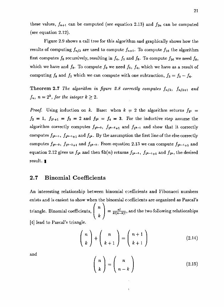
these values, fn+1 can be computed (see equation 2.13) and f2 can be computed
(see equation 2.12).
Figure 2.9 shows a call tree for this algorithm and graphically shows how the
results of computing fn/2 are used to compute /n+1. To compute f16 the algorithm
first computes 18 recursively, resulting in h, h and f8. To compute f16 we need f8,
which we have and f9. To compute f9 we need h, 14, which we have as a result of
computing f8 and h which we can compute with one subtraction, 13 = f5 14.
Theorem 2.7 The algorithm in figure 2.8 correctly computes fro, A/2+1 and
n = 2k, for the integer k > 2.
Proof. Using induction on k. Base: when k 2 the algorithm returns 121 =
12 = 1, 121+1 = h = 2 and 122 = h = 3. For the inductive step assume the
algorithm correctly computes f2k-2, f2k_2+1 and f2k-i and show that it correctly
computes f2k -,, f2k-1+1 and f2k. By the assumption the first line of the else correctly
computes f2k_2, f2k-2+1 and f2k-i. From equation 2.13 we can compute f2k_14.1 and
equation 2.12 gives us f2k and then fib(n) returns f2k -1, f2k-1+1 and f2k, the desired
result. I
2.7 Binomial Coefficients
An interesting relationship between binomial coefficients and Fibonacci numbers
exists and is easiest to show when the binomial coefficients are organized as Pascal's
triangle. Binomial coefficients,
[4] lead to Pascal's triangle.
and
n!
kk!(n-k)!, and the two following relationships
n n +1
k +1 k +1
) n:
(2.14)
(2.15)
22
n
0 1
1 1 1
2 1 2 1
3 1 3 3 1
4 1 4 6 4 1
5 1 5 10 10 5 1
k 0 1 2 3 4 5
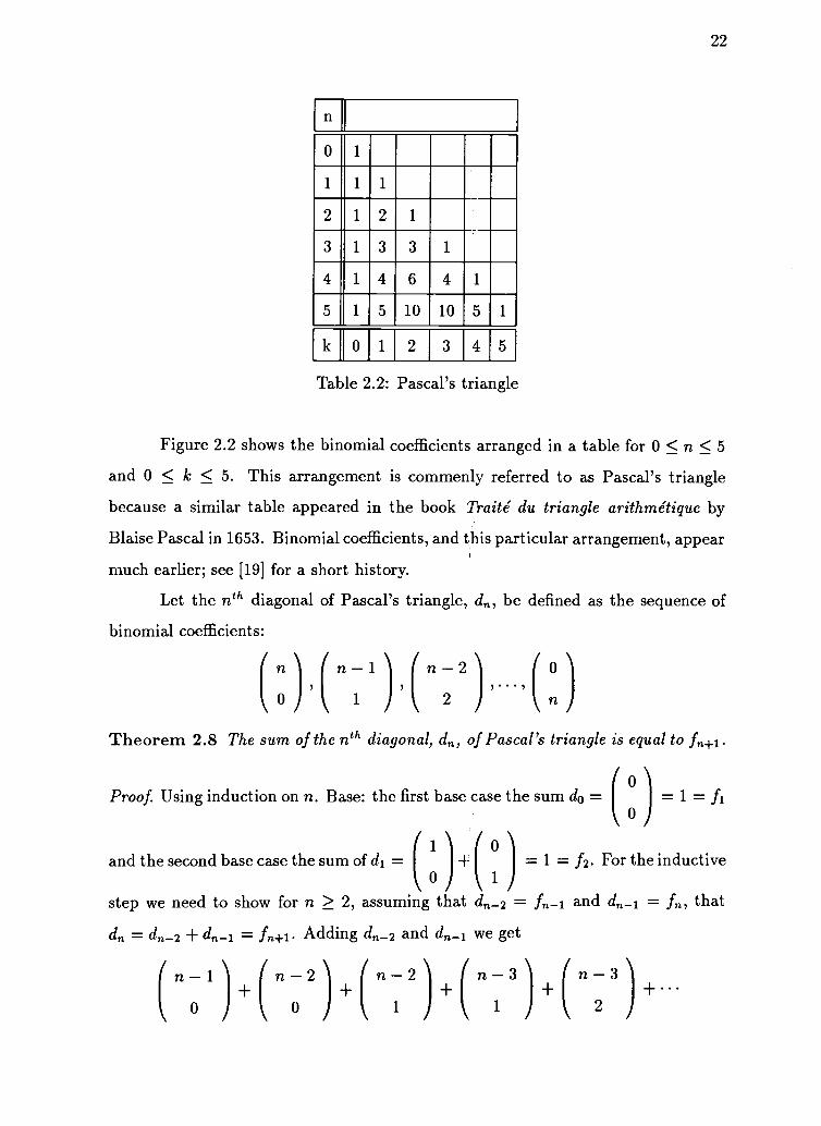
Table 2.2: Pascal's triangle
Figure 2.2 shows the binomial coefficients arranged in a table for 0 < n < 5
and 0 < k < 5. This arrangement is commenly referred to as Pascal's triangle
because a similar table appeared in the book Traite du triangle arithmetique by
Blaise Pascal in 1653. Binomial coefficients, and this particular arrangement, appear
much earlier; see [19] for a short history.
Let the nth diagonal of Pascal's triangle, dn, be defined as the sequence of
binomial coefficients:
n n 1 ) n 2 ) 0
2 n
Theorem 2.8 The sum of the nth diagonal, d, of Pascal's triangle is equal to ffl+1.
Proof Using induction on n. Base: the first base case the sum do = =1 =fi
1 0and the second base case the sum of d1 = + = 1 = 12. For the inductive(
0 1
step we need to show for n > 2, assuming that dn_2 = fn_i and dn_1 = fn, that
do = dn_2 dn_1 = fn+1. Adding dn_2 and dn_1 we get

Since
23
( 0 0
n 2 ) n 1
( (
n 1
0
(we can replace the first term with
pairs of terms to get
n n 1
1
n
0 )
=1O
and apply equation 2.14 to all subsequent
n 2 ) ( 1
2 n 1
( 0Since n > 2 and = 0, the sum of do is equal to the sum of dn_2 plus the
n 1
sum of dn_i. So, since dn_2 = fn-1 and dn_2 = fn, do = 4-2 + 4-1 = In-1 + =
In+1 I
The algorithm to compute In is to take the sum of dn_1. The interesting
question is "Is there a fast way to compute binomial coefficients?". The standard
method of computing binomial coefficients is [lit]:
and
and if n < k
k)=-(;c1
=1
=0
P. Goetgheluck [14] presents an algorithm to
torization ofn
. His algorithm is presented in
1(2.16)
1
compute the prime power fac-
figure 2.10, E is the power of

24
input n, k and p
E 4 0, r 4-- 0
if p > n k then E 4 1; end.
if p > n/2 then E 4 0; end.
if p * p > n then if n mod p < k mod p then E 4 1; end.
Repeat
a 4 n mod p
n I pi
b 4 (k mod p) r
k 4 Yelp]
if a < b then E 4 E 1,r 4- 1
else r 4- 0
until n = 0
Figure 2.10: Goetgheluck'3 algorithm

the prime p in the factorization of
25
n.
nKnowing the factors of for all
p < n the binomial coefficient can be computed by taking the product of pr. for all
pi < n.
2.8 Generating function
We can use a generating function, G(z), to represent the entire Fibonacci sequence.
Let
G(z) = fo fiz f2z2 + = E fnzn.n>0
zG(z) = foz1 + fiz2 f2z3
z2G(z) = foz2 fiz3 f2z4
By computing G(z) zG(z) z2G(z) we get
G(z) zG(x) z2G(z) = foz° + (fi fo)? + (12 fi fo)z2 +
(f3 f2 ft )z3 +
G(z)(1 z z2) = z +0z2 0z3 +
G(z) = z /(1 z z2)
(2.17)
(2.18)
We can evaluate the polynomial G(z) = z /(1 z z2) at the roots ofunity up 4.01 w2, ,.", getting the values vo, v1, v2, , vn_i. To find the
coefficients, the Fibonacci numbers, perform the inverse Fourier transformation. To
find a specific coefficient, fk, use only the k 1 row of the Fourier matrix, _F.
n-1fn = E Vi
i=0
2.9 Product of Factors
The evaluation of the generating function above produced approximations of fn.
Several small terms were involved in computing the approximation and they were

26
eliminated one by one since they became very small as n grew. From empirical
observations eliminating the small terms seemed to improve the approximation and
when all of the small terms were gone the results seemed to be exact Fibonacci
numbers.
The formula that was suggested is
f2' =HNi
where
= 2, /(31 = 3- (2.19)
The numbers th , , A are a factorization, although not necessarily prime, of
f2s. The Fibonacci relationship this suggests is
(Ln 2
2( -1)'
To show this is true, by equation 2.4,
f4n
f2n
and, remembering that Al A2 = 12
(ff2nn)
1
= A??1
2
A2n )2n ) 22(-1)n = Ar221, 2(-1)n
= (A7 A2)2 2(-1)n
= A?n 2(A1A2)n ,1n 2(-1)"
= An +
So, equation 2.20 is correct.
(2.20)
Lemma 2.1 The algorithm in figure 2.11, when given a positive integer i, correctly
computes a factorization of f21 +1.
Proof Using induction on i. Base: when i = 1 the algorithm returns a list with the
one element f2T+1 = f4 = 3 so the base case is correct. For the inductive step assume

27
beta (i)
if i = 1 return the list (3)
else
temp 4 beta (i - 1)
last 4- last element of temp
newbeta 4 temp * temp - 2
return the list temp with newbeta appended to the end.
Figure 2.11: Algorithm to compute /3
fib (i)
if i = 0 return 1
else if i = 1 return 1
else
let temp = beta (i - 1)
return the product of all elements in temp
Figure 2.12: Algorithm to compute f2, using 3

28
that the algorithm correctly computes a factorization of f2. and show that for i it
correctly computes a factorization of f2,+1. Since n = 2i, i > 1, n is even and, by the2
assumption, 7,t-;2 is computed correctly, 2.20 tells us that (I:it-112) 2( -1)n =
Since n is even (-1)n = 1 and 2( -1)n becomes -2 so the step in the algorithm
that computes newbeta is correct. So .9u- can be computed and is added as the
last element in the list temp and since the list temp, by the assumption, already
contains a factorization of fn and fn ,tja = f2n the algorithm correctly computes a
factorization of f2.+1. 1
Theorem 2.9 The algorithm in figure 2.12 corg.ectly computes fn, n = 2i, for the
non-negative integer i.
Proof If i = 0 the algorithm correctly returns f2° = f1 = 1, if i = 1 the algorithm
correctly returns f21 = f2 = 1. For i > 2 the algorithm returns the product of
the elements returned by the call to beta (i-1). By lemma 2.1 beta (j) correctly
computes a factorization of fv+i so this algorithm correctly computes fr.
The algorithm in figure 2.12 could generate the sequence of Fibonacci num-
bers
f4, fs, f16, , frby printing the results of each multiplication. This can be generalized to generate
the sequence
f4+k)fs+k, fie+k, , f2' +k
for any integer k using the relation
f2j+k = fk
To show this is true, by equation 2.4,
12j-Fk(X2' A3i)
= (Ari+k- A2`-' +k) (Ar Ari)
Or-1+k (AT1 A22.1 -2
(2.21)
2` A2i-1 12i-l-f-k 12i-11-k 12i-1 2i-j-kA2 (a1 Ak)= Al '2 f 1 2
2i+kA1
2'+kA2 ()1A2) A2 (Ai A2)22 k Oki A2)

fib (n)
sI 4 [log n] 1
/3-sequence N, /31, /32, , 081-1
fl-sequence 4-- fl, f3, f7, ,
f2-sequence 4 / 2 f4 /8, , f231
fib-help (n sI fl-sequence f2-sequence)
Figure 2.13: Product of factors algorithm to compute any fn
since A1 )12 = 1
= A?i +k +k a2 + a1 (Ak1 A2)
29
By choosing k = 0 we get the sequence generated by the algorithm in fig-
ure 2.12
12, 14, 18, 116,
and by choosing k = 1 we get the sequence
13, 17, 115,
The sequences
11, 13, 17, , (2.22)
and
12, ft, 18, , hi (2.23)
and equation 2.10 lead to the algorithm presented in figure 2.13
Lemma 2.2 The algorithm presented in figure 2.14 will, when given a non-negative
integer n, expo = [log ni 1, the sequence f1i 13, 17, . , f2expo_i, and the sequence
12,14, 18, , f2e., correctly compute fn.

30
fib-help (n expo flseq f2seq)
if n = 0 return 0
else if n = 1 return 1
else if n = 2 return 1
else
return flseq[expo] fib-help (n 2"P°, rog(n 2"P°)1 1, flseq, f2seq)
f2seq[expo] fib-help (n 2"P° + 1 Flog(n 2"P°)1 1, flseq, f2seq)
Figure 2.14: Recursive section of algorithm to compute any fn
Proof. Using induction on n. Base: when n = 0, fo = 0 is returned, when n = 1,
fl = 1 is returned, and when n = 2, 12 = 1 is returned. For the inductive step
assume that the algorithm correctly computes fi for all 0 < j < n and show that
the algorithm correctly computes fn+1. Since the ith element of fl-sequence is f2i_1,
the ith element of the f2-sequence is f2i, and the assumption; the algorithm will
return the value f2exP°-1 fn-2exP° f2exP° fri-2exP°4-1 By equation 2.10 this is fn. I
Theorem 2.10 The algorithm presented in figure 2.13, when given an integer n,
3 < n, will corectly compute h.
Proof. The three sequences /3-sequence, fl-sequence, and f2-sequence can be correctly
computed using equations 2.19 and 2.21. By lemma 2.2, the algorithm correctly
computes h.
31
Chapter 3
Results and Analysis
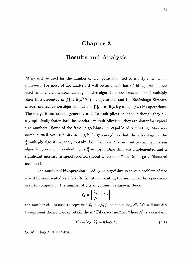
M (n) will be used for the number of bit operations used to multiply two n bit
numbers. For most of the analysis it will be assumed that n2 bit operations are
used to do multiplication although better algorithms are known. The I multiply
algorithm presented in [1] is 0(7/10423) bit operations and the Schiinhage-Strassen
integer multiplication algorithm, also in [1], uses 0(n log n log log n) bit operations.
These algorithms are not generally used for multiplication since, although they are
asymptotically faster than the standard n2 multiplication, they are slower for typical
size numbers. Some of the faster algorithms are capable of computing Fibonacci
numbers well over 105 bits in length, large enough so that the advantage of the
Imultiply algorithm, and probably the Schonhage-Strassen integer multiplication
algorithm, would be evident. The a multiply algorithm was implemented and a
significant increase in speed resulted (about a factor of 7 for the largest Fibonacci
numbers).
The number of bit operations used by an algorithm to solve a problem of size
n will be represented as T (n). To facilitate counting the number of bit operations
used to compute fn the number of bits in fn must be known. Since
Anfn=
the number of bits used to represent fn is log2 fn or about log2 Ali. We will use Nn
to represent the number of bits in the nth Fibonacci number where N. is a constant.
Nn = log2 Ai = n log2 Ai (3.1)
So Ar = log2 Al ti 0.69424.

32
3.1 Natural recursive
The number of bit operations required to compute fn using the algorithm in fig-
ure 2.1 is the sum of the number of bit operations to compute fn_1 plus the number
of bit operations to compute fn_2 plus the number of bit operations to add f.--1
and fn_2. This gives the recurrence relation
with initial conditions
Tn = Tn-1 Tn-2 N.12
To = 0
= 0
Since this is a linear constant coefficient difference equation the general solution can
be writtenk
X = V + E ai Ari`
i=i
where v is the particular solution, Ai is the ith root of the characteristic polynomial
of the difference equation, and the a's are constants.
Solving the recurrence relation, we find the roots of the characteristic poly-
nomial.
A2 1 = 01 +
2
1 -V75A2
2
Find the particular solution
Vn = CiArn + C2
(Ci.A.rn + C2) (CiAr(n 1) + C2) (CiAl (n 2) + C2) = Nn
Cl = 1C2 = -3Ar

Solve the following two equations for al and a2
To Vo = ai A? + a2A2°
a2A1
Giving
(3 4 3A1
A2 - Al
N (4 3A1)o2 =112
Let /3 = Ar (3 If .11,) So
33
Tn = + (3.Al #),V22. Arn 3.Ar (3.2)
Since 0 < /3 < 3 both al and a2 are positive. Since 0 < al, 0 < a2, 1 < A2 < 0,and 1.5 < < 2 the number of bit operations used by the algorithm in figure 2.1
is 0(An. Since Al > 1.5 and this algorithm is exponential in n, it is unlikely to be
useful for large n.
3.2 Repeated addition
Using the algorithm presented in Figure 2.2 each 2 < i < n, is computed with
the addition fi = fi-i + fi_2. Each of these additions uses Ar(n 1) bit operations
so the total number of bit operations needed to compute fn is
T(n) = T(n 1) + Ar(n 1), T(0) = 0, T(1) = 0
E Ar(i 1)i=2
n-2= + 1)
i=0
((n 2)2 (n 1)).Ar(n 1)
= Ar n2 n)2 2) (3.3)

34
For the generalized Fibonacci numbers, fn, a similar algorithm using k ad-
ditions at each step will use about Ari-cf'2 bit operations.2
Tk(n) = Tk(n 1) (k 1)Ar(n 1), T(0) = 0, T(1) = 0
1)i=2
((k 1)(n2
2)(n+ 1)
((k 21)n2 (k 1)n)2
(3.4)
When k = 2 (the Fibonacci numbers) we get
T2(n) = Ar(n2 n)
2 2
the same as equation 3.3 above.
The algorithm presented in Figure 2.3 for computation of f4e decreases the
number of bit operations by a factor of (k 1)/2. The value of .Ar will be different
for different values of k so when k 2 the constant will be denoted NI. Ark will
always be less than one. Since the multiply is by two, a shift can be used instead
and the computation of the next Alf will use two /1/1(n 1) bit instructions, a shift
and a subtract.
Tk(n) Tk(n 1) + 2.1111(n 1), T(0) = 0, T(1) = 0
= 2Ark(i 1)i=2n-2
2.Ark(i + 1)i=0
n-2= 2Nk(n- 1) +2Nk >i
i=o
(n 2)(n 1))= 2 A r k 1 +
2
= Ark(n2
3.3 Binet's Formula
(3.5)
There are three operations that must be considered to count the bits operations
needed to compute fn using the algorithm presented in figure 2.4. The Ain + log n

35
bits of the square root of five must be computed, an Ain + log n bit number must
be exponentiated to the nth power, and a Nn + log n bit division must be done.
The can be computed using log Ain-Flog n iterations of Newton's method
[13]. Each iteration of Newton's method requires a division and the length of the
significant result doubles with each iteration. It will be assumed that a division
requires n2 bit operations, denoted as D(n).
T(n) = T(n12)-F D(Ain12)(Nn)2 (Nn)2 (Ain)2
4 16 64(Ain)2
221
= (Nn)2 t (1)8
(Ain)23
(3.6)
During each log i iterations of the exponentiation, only the most significant
Nn + log n bits need be kept. Therefore the time needed to perform the exponen-
tiation is log n(Afn + log n)2 bit operations.
The operands for the final division are Ain bits and Ain + log n bits so the
division will take less than (\n + log n)2 bit ope7ations.
the total number of bit operations using the algorithm presented in figure 2.4
will be dominated by the log n(Ain + log n)2 bit operations used by the exponenti-
ation giving O(log n M(n)) bit operations.
3.4 Matrix Multiplication Methods
In this section, and the next, the matrix algorithms and the extended N. N. Vorob'ev
algorithm will be analyzed producing a sequence of the number of bit operations
to compute fn from 8(n3 )2 down to 5( 1N)2. Similar methods are used to find the
running time for each of the algorithms in this section and the next so one general
introduction is presented here and the specifics' for each algorithm is presented in
the appropriate sections.

36
All of the algorithms use some number of additions and some other number
of multiplications. Since the additions can be done in time linear with respect to the
size of the operands and it will be assumed that multiplication requires n2 time for
operands of size n, the bit operations resulting :rom the additions will be ignored
and only those resulting from multiplications will be counted.
The simple matrix multiplication algorithm introduced in the first course in
linear algebra requires row column multiplications of size n/2 for a resulting matrix
with elements of size n. In the case of computing
An =( 1 1 ) fn+i fn
1 0 fn -1
this method would require eight multiplications of size n/2 to compute the matrix
(In+i In
fn fn -1
from the matrix
(fn/2+1 fn/ 2
fn/2 fn/2-1
by squaring the second matrix. The number of bit operations needed to compute
the matrix containing fn using the above method with eight multiplies is 8.M(nAr)3
T (n) = T (n /2) + 8M (Ar n / 2)
= 8M(A1 n/2) 8M(Afn /4) 8M(JVn /8) +8(Nn)2 8(Nn)2 8(.?1in)2
4 16 64
= 8(Nn)24
= 8(Nn)2
8(Arn)2
3(3.7)
Since we can compute the first row of An+1 from An using four multiplications
and the second row can be computed using only an addition and four multiplications

37
are needed. Using a sequence of operations similar to those above we get 4.m(nAr)3
bit operations.
T(n) = T(n12)-1- 4M(Arn/ 2)4(Arn)2
3
3.4.1 Three Multiply Matrix Method
(3.8)
The three multiply matrix method presented in figure 2.6 performs three half size
multiplies, three additions, and calls itself recursively with half size arguments.
Since we are ignoring the additions we get M(nAr) bit operations.
T(n) = T(n12)+3M(Arn12)
= 3M(Ain/2) 3M(Arn1 4) + 3M(Arn/8) +3(Nn)2 3(Ain)2 3(Nn)2
4 16 643(Ain)2=
2211=1
= 3(Nn) (1)14
= 3(.Arn)2 13
(./Vn)2 (3.9)
3.4.2 Two Multiply Matrix Method
The two multiply matrix method presented in figure 2.7 does two half size multiplies,
four additions, one shift, and calls itself recursively with a half size argument. The2 M(Arn)number of bit operations used by this algorithm is 3
T(n) = T(n /2) 2M(Arn/2)
= 2M(Ain/2) 2M(Ain/4) 2M(Arn/8) +2(Arn)2 2(Ain)2 2(.Afn)2
4 16 642(Arn)2= - 2211=1

(1)'= 2(.Arn)2E4
= 2(Nn)2
32(.Afn)2
3
3.5 Extended N. N. Vorob'ev's Method
38
(3.10)
By using the results of computing f21 to compute f2i+1 the algorithm presented in
figure 2.8 is able to replace one 2 bit multiply with two a bit multiplies each time
it is called. The extended N. N. Vorob'ev algorithm uses m(Ar2 n) bit operations.
T(n) = T(n/2) M(Arn/2) 2M(Ain/4)
111 (Ain/2) 3M(Arn/4) 3M(Arn/8) +(Nn)2 3(Nn)2 3(Nn)2
4 16 64(Nn)2 cx, 3(Nn)2
4 1=2 22s
43(Nn)2 (1)i(Nn)2
(Arn)2 3(Nn)24 I 12
(Nn )2
2
3.6 Product of Factors
(3.11)
The product of factors algorithm presented in section 2.9 uses two multiplies at each
recursive call. One multiply is to compute Oi_i by squaring a n/4 bit number and
the other is to compute fit by multiplying Oi_i by the product of /31,02, , 0i-2
both n/2 bit numbers. The number of bit operations this algorithm uses to compute
the nth Fibonacci number is 5.111(Arn)12
T(n) = T (n I 2) + (.Ar n 12) + AI (N. 7 11 4)

= M(Ain12)+2M(Arn14) +2M(Arn18) +(Ar n)2 2(JVn)2 2(JVn)2. + -I- +
4 16 64(Ar
4
n)2. + 2(Nn)2 2 E (4)i=2
\ 2 (Ain)2= kjv4n)
12+ 2 '
5(Ain)212
3.7 fn for any n using Product of Factors
The algorithm in Figure 2.13 computes the three sequences
01, 021 /331 13i
13, 17, 115, , f2,--1
ft, 18, 116, , hi
39
(3.12)
for i = rlog2 n1 1. The worst case for computing these sequences is n = 2` + 1
where the size of i3i is about half of the size of fn with /2. -1 and f2. about the same
size as fn. The best case for this computation is n = 2i, where is about one
fourth the size of fn with f2.-1 and f2. half of the size of fn. We will see that the
best and worst cases are switched for the second phase of this algorithm.
In the worst case the number of bit operations for the the first phase, com-
puting the three sequences, of the algorithm presented in figure 2.13 is
T(n) = T(n12)+2M(Arn) M(Ain12)
2M(.Arn) 3M(Arn12) + 3M(Ain14) +3(Air)2 3(Nn)2
= 2(Arn)2 +16
2(Arn)2 E) 3(Ar2:)2
= 2(.Arn)2 3(A1n)2 t= 2(A.rn)2 + (N.n)2

40
= 3(Nn)2 (3.13)
In the second phase of the algorithm (the call to fib-help) the various values
of the two sequences are multiplied together to get fn. In this phase the worst case
will be when the numbers being multiplied together are about the same size, or
about one half the length of fn. The number of bit operations for the second phase
is at most
T(n) T(n /2) 2M(Ain/2)
= 2M(.Arn/2) 2M(Arn/4) 2M(Arn/8) +2(Ain)2 2(Nn)2 2(Nn)2
4 16 642(Nn)2=
4-4 22ii=1
= 20(.71)2 ct° (1)ii=i 4
= 2(Nn)2.1
2(Nn)23
(3.14)
So, the worst case number of bit operations for the algorithm presented in figure 2.13
is certainly less than 11(ji(lit 23
3.8 Matrix Method of Gries and Levin
The algorithm of Gries and Levin presented in section 2.4 exponentiates the k x k
matrix A using only k2 multiplications at each step. Each iteration of the algorithm
doubles n so only log n iterations are required to compute fn. This leads to the
equation
Tk(n) = Tk(n 12) k2 M(Arn 12)
= k2M(ArnI2)+ k2111(Ain14)-F k2M(ArnI8) +k2(Nn)2 k2(A/72)2 k2(Ain)2
4 16 64(1 y
= k2(Nn)2 4/

k2(Ain)23
For k = 2 (the fibonacci sequence)
T2(n) =4( Arn)2
Or4.M (N n)
3
3.9 Binomial Coefficients
41
(3.15)
(3.16)
Computing fn+i by taking the sum of the nth diagonal of Pascal's triangle requires
computing the n +1 binomial coefficients in the nth diagonal. The two methods pre-
sented in section 2.7 will be analyized, but since the optimal method of computing
binomial coefficients is not known there may be better algorithms.
Using the standard method of computing binomial coefficients, see equa-
tion 2.16, requires computing k(n k) ii2- elements of Pascal's triangle. There are
k(n k) elements added to compute but since Pascal's triangle is symmet-
rical, Equation 2.15 only the elements on one side of the center of Pascal's triangle
need to be computed. From the diagram in figure 3.1 it can be seen that the largest
number of elements will need to be computed when k = 'it. These elements also
have the largest values since they are closest to the center of Pascal's triangle. The
total number of elements of Pascal's triangle that need to be computed in order ton
compute( )
isk
and when k =2
12'-
n(n k)(n In/2 ki)2
4
n2 (n Li 1)
2
2 4
=
=
n2 n2
2 4n2
4

1n2
n
n
42
Figure 3.1: Elements of Pascal's triangle used to compute a binomial coefficient

43
So, in the worst case, there are 74 elements to be added and each of these elements
must be less than n bits long since the sum of the nth row of Pascal's triangle is
equal to 2n or
tz. n =k
therefore at most 11: bit operations need to be done to compute
nk
To compute fn a complete diagonal of Pascal's triangle must be computed.
Since the diagonal rises to the right all of the elements in the nth diagonal will be
computed if2n
is computed. This will take, at most, IV = n3 bit operations
to compute. Clearly, this is a gross overestimate of the time required to compute
f by taking the sum of the nth diagonal of Pascal's triangle.
A different way to compute binomial coefficients is with Goetgheluck's al-
gorithm. Each call to the function given in figure 2.10 performs logy n iterations.
During each iteration two divisions of the same size are done, the size decreasing
by a factor of p each iterations. The number of bit operations done by one call is
less than
log,, n
E2 -7 P= Pt
logy n
E 2 n.pi 1
n n nn + + + + + 1pl p2 p3
Since the sum will be the largest when the prime number, p = 2, a call to the
function in figure 2.10 will take no more than
n n n+
2+
4+
8+ 1
= 2n
bit operations. There will be at most n 1 calls made to the function, so the resulting
number of bit operations is < n2.
1The actual number is the number of primes < n or about iongn calls, but this is a slight under-
estimate and using n will not change the order.

44
Once the factors are computed they must be multiplied together to form
the binomial coefficient. In the worst case we would have to multiply two half size
numbers to get the result, and four quarter size numbers to get the two half size
numbers and so on.
T(n) = 2T(n/2) M(n/2)
M(n/2) 2M(n/4) 4M(n/8) +n2 n2 n2
4+
16+
32+
n2 (4 )i
n2
3
Adding the time to compute the factors and the time to multiply the factors, we
get the time to compute a binomial coefficient < 4+2.
To compute fn+i, the N1 binomial coefficients of the dth diagonal need to
be computed.
T(n) La 3i=n/2
n/2 /1) 2
3 2)4 71/2 n2
3 4-4 4
4 0(2 +1)('21+1) n3\3 6 2
n3 5n2n
Again, this is gross overestimate of the number of bit operations needed to
compute fro.i and is not useful to compare with number of bit operations needed
to compute fn+i using the standard method.
45
Algorithm Constant
Repeated Addition 4.223 E -6
Product of Factors (any fn) 3.273 E -8
Binet's Formula (any fn,) 1.06 E -1
Binet's formula (fn, n = 2k) 7.038 E 5
Product of Factors (A, n = 2k) 1.633 E 8
3 Multiply Matrix 3.950 E 8
2 Multiply Matrix 2.667 E 8
Extended Vorob'ev 1.983 E 8
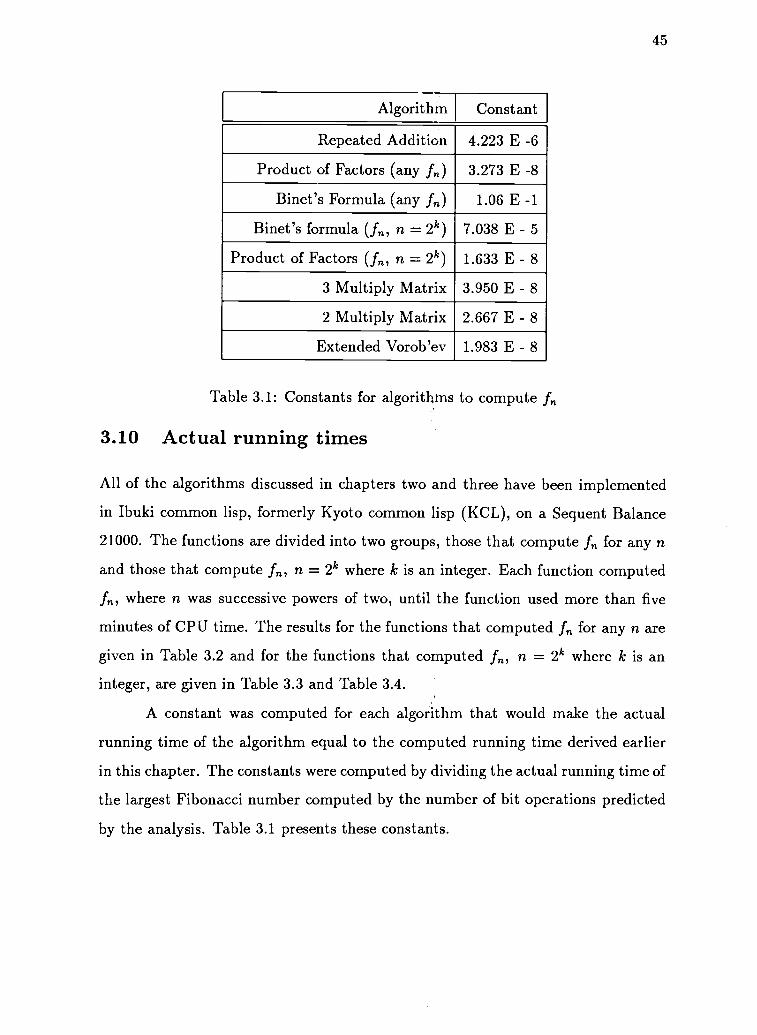
Table 3.1: Constants for algorithms to compute fn
3.10 Actual running times
All of the algorithms discussed in chapters two and three have been implemented
in Ibuki common lisp, formerly Kyoto common lisp (KCL), on a Sequent Balance
21000. The functions are divided into two groups, those that compute fn for any n
and those that compute fn, n = 2k where k is an integer. Each function computed
fn, where n was successive powers of two, until the function used more than five
minutes of CPU time. The results for the functions that computed fn for any n are
given in Table 3.2 and for the functions that computed fn, n = 2k where k is an
integer, are given in Table 3.3 and Table 3.4.
A constant was computed for each algorithm that would make the actual
running time of the algorithm equal to the computed running time derived earlier
in this chapter. The constants were computed by dividing the actual running time of
the largest Fibonacci number computed by the number of bit operations predicted
by the analysis. Table 3.1 presents these constants.

46
log n
Repeated
Addition
Product; of
Factors
comp r act
Binet's
Formula
comp actcomp act
2 0.00-0.00 0.00-0.00 3.82-0.08
3 0.00-0.00 0.00-0.02 12.82-0.13
4 0.00-0.02 0.00-0.02 42.40-1.60
5 0.00-0.00 0.00-0.02 145.11-44.28
6 0.02-0.03 0.00-0.03 519.43-519.43
7 0.07-0.07 0.00-0.05 na-na
8 0.28-0.22 0.00-0,05 na-na
9 1.10-0.62 0.01-0,08 na-na
10 4.42-5.17 0.03-0.17 na-na
11 17.71-16.73 0.14-3.28 na-na
12 70.84-71.30 0.55-6.97 na-na
13 283.39-279.52 2.20-9.60 na-na
14 1133.62-1133.62 8.79-17.45 na-na
15 na-na 35.14-49.92 na-na
16 na-na 140.57-154.40 na-na
17 na-na 562.28-562.28 na-na
Table 3.2: Running time to compute fn for any n in CPU seconds

47
log n
Binet's
formula
Product of
Factors
comp act comp act
2 0.00-0.02 0.00-0.00
3 0.01-0.02 0.00-0.02
4 0.03-0.03 0.00-0.00
5 0.10-0.05 0.00-0.00
6 0.34-0.13 0.00-0.00
7 1.28-0.75 0.00-0.00
8 4.91-14.83 0.00-0.02
9 19.10-11.10 0.00-0.02
10 75.25-77.82 0.01-0.05
11 298.38-287.70 0.07-0.12
12 1187.73-1187.73 0.27-0.37
13 na-na 1.10-1.23
14 na-na 4.38-4.60
15 na-na 17.53-17.77
16 na-na 70.12-73.98
17 na-na 280.47-280.22
18 na-na 1121.88-1121.87
Table 3.3: Running time to compute fn, n = 2k, in CPU seconds, part 1

48
log n
3 Multiply
Matrix
2 Multiply
Matrix
Extended
Vorob'ev
comp act comp act comp act
2 0.00-0.02 0.00-0.02 0.00-0.00
3 0.00-0.02 0.00-0.00 0.00-0.00
4 0.00-0.00 0.00-0.02 0.00-0.02
5 0.00-0.00 0.00-0.00 0.00-0.00
6 0.00-0.02 0.00-0.02 0.00-0.00
7 0.00-0.03 0.00-0.03 0.00-0.02
8 0.00-0.05 0.00-0.05 0.00-0.03
9 0.01-0.05 0.01-0.05 0.01-0.03
10 0.04-0.10 0.03-0.10 0.02-0.07
11 0.17-0.28 0.11-0.25 0.08-0.18
12 0.66-0.83 0.45-0.70 0.33-0.47
13 2.65-2.92 1.79-5.62 1.33-1.58
14 10.60-14.52 7.16-7.77 5.32-9.23
15 42.41-42.85 28.63-29.35 21.29-21.63
16 169.66-172.65 114.54-117.97 85.17-84.98
17 678.63-678.63 458.15-458.15 340.68-340.68
Table 3.4: Running time to compute fn, n = 2k, in CPU seconds, part 2

49
Chapter 4
Redundant Information
Since so few of the integers are Fibonacci numbers we would expect redundant
information in the integer representation of the Fibonacci numbers. If we could
understand the structure of this redundancy, we could take advantage of it in com-
puting fn by using a representation using fewer bits than the integers. This chapter
will present three compression methods that were run on a string of bits represent-
ing the sequence of ascending Fibonacci numbers. The results of compressing the
Fibonacci sequence yielded no insights into any redundant structure that might ex-
ist in the Fibonacci sequence. The compression algorithms behaved as they would
if given a random sequence of bits to compress, so the bits of the Fibonacci se-
quence were tested as a random sequence. The three tests for randomness that
were performed indicated that the sequence of bits was random.
The final section of this chapter looks at the Fibonacci numbers in a different
arrangement, instead of placing the binary representation of the Fibonacci numbers
end to end, a binary sequence was constructed from the bth bit of each Fibonacci
number. Arranging the Fibonacci numbers in this manner shows that the bth bit
forms a cycle of length 3 2b. Unfortunately, the cycle length is exponential in b,
the bit position, and since the number of bits in fn grows linearly with n, the cycles
seem to only be useful in computing the lower bits in fn. If we could compute
the value of the mth bit in the bth cycle quickly (i.e., without computing the entire
cycle) we might be able to compute fn quickly. Redundancy in the bth cycle was
investigated and found but efforts to explain it have not yet been successful. This
is described in the final section of this chapter.

50
4.1 Compression
The sequence of bits that will be compressed is obtained by writing, in binary, each
Fibonacci number end to end. The bits of each ff, are written in reverse order, that
is the most significant bit is to the right. The start of the sequence would be
fl f2 13 f4 15 f6
1 1 2 3 5 8
1 1 01 11 101 0001
1101111010001
The bits of the individual fn are in reverse order so that when the sequence is read
from left to right the low order bit of fn will be read first, but the order should not
be important as long as it is consistent.
The sequence of Fibonacci numbers were made available to the data com-
pression algorithms in two forms, one bit at a time or one byte at a time. When
a compression function requests the next source character, the leftmost unused bit
(byte) in the sequence is removed from the sequence and is returned to the calling
function. The next Fibonacci number is computed when the current source of bits
(bytes) have been exhausted. This allows the possibility of analyzing very long
sequences.
Terry Welch [38] discusses four types of redundancy: character distribution,
character repetition, high usage patterns, and positional. If some characters appear
more frequently than others in a sequence that ; equence is said to have character
distribution redundancy. For example, in the English language the characters 'e'
and ' occur with greater frequency than the character 'z'. Character repetition
redundancy occurs when the same character appears several times in succession.
Frequently, files with fixed size records will use a blank, or some other distinguished
character, to fill the records; these filler blanks are frequently a source of character
repetition redundancy. High usage pattern redundancy is an extension of character
distribution redundancy, instead of noting that some individual characters appear

51
Compression Ratio
k integer r Fibonacci random
128 0.508 0.821 0.533 0.533
256 0.577 2.667 0.520 0.561
512 0.569 2.510 0.520 0.547
1024 0.580 2.081 0.527 0.537
2048 0.616 2.216 0.524 0.532
4096 0.639 2.306 0.531 0.527
8192 0.680 2.421 0.530 0.534
16384 0.712 2.447 0.531 0.530
32768 0.747 2.496 0.532 0.531
Table 4.1: Compression ratios of Ziv-Lempel for various sources
more frequently than others, it is noted that some groups of characters appears more
frequently than other groups of characters. A sequence is positionally redundant
when the same character appears at the same position in each block of data. An
example of positional redundancy would be a file containing a list of numbers of the
form "XXXX.YY" since the '.' always appears as the fifth character. Positional
redundancy will be important in section 4.3.
4.1.1 Ziv Lempel Compression
The Ziv Lempel (ZL) compression algorithm, [40,41,42], along with the LZW com-
pression algorithm, [38], will be considered and the results of applying them to the
sequence of Fibonacci bits will be discussed in this section.
A formal description and analysis of the Ziv Lempel compression algorithm
is in [41], what follows is an informal presentaton of the algorithm. If we have a
array of characters, S, of length k and an integer j, 1 < j < k, then we can match,
character by character, the string at S[1] with the string starting at S[j]. Let L(i)

52
Compression Ratio
k integer 2' Fibonacci random
128 0.731 1.438 0.677 0.703
256 0.776 2.393 0.753 0.755
512 0.806 3.483 0.791 0.782
1024 0.861 4.697 0.811 0.811
2048 0.838 6.564 0.841 0.830
4096 0.848 8.480 0.842 0.842
8192 0.854 11.977 0.851 0.849
16384 0.866 15.326 0.859 0.858
32768 0.870 21.530 0.868 0.867
Table 4.2: Compression ratios of the modified Lempel-Ziv-Welch algorithm
Compression Ratio
k integer 2' Fibonacci random
128 0.871 1.707 0.871 0.871
256 0.880 3.413 0.880 0.880
512 0.838 5.069 0.839 0.845
1024 0.815 7.758 0.809 0.805
2048 0.783 11.253 0.763 0.765
4096 0.749 16.190 0.725 0.725
8192 0.721 22.506 0.698 0.694
16384 0.718 30.972 0.678 0.678
32768 na 43.691 na na
Table 4.3: Compression ratios for Unix Ziv-Lempel implementation
53
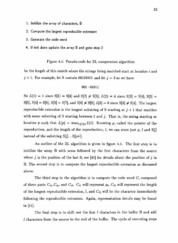
1. Initilize the array of characters, B
2. Compute the largest reproducible extension
3. Generate the code word
4. If not done update the array B and goto step 2
Figure 4.1: Pseudo-code for ZL compression algorithm
be the length of this match where the strings being matched start at location i and
j 1. For example, let S contain 00101011 and let j = 3 so we have
001 01011
So L(1) = 1 since S[1] = S[4] and S[2] S[5]; L(2) = 4 since S[2] = S[4], S[3] =
S[5], S[4] = S[6], S[5] = S[7], and S[6] 0 S[8]; L[3] = 0 since S[3] 0 S[4]. The largest
reproducible extension is the longest substring of S starting at j 1 that matches
with some substring of S starting between 1 and j. That is, the string starting at
location p such that L(p) = maxi<i<p L(i). Knowing p, called the pointer of the
reproduction, and the length of the reproductio:1, 1, we can store just p, 1 and S[j]
instead of the substring S[j]...S[j+1].
An outline of the ZL algorithm is given in figure 4.1. The first step is to
initilize the array B with zeros followed by the first characters from the source
where j is the position of the last 0, see [41] for details about the position of j in
B. The second step is to compute the largest reproducible extension as discussed
above.
The third step in the algorithm is to compute the code word Ci composed
of three parts Cil, Ci2, and Ci3. Cal will represent pi, Cie will represent the length
of the longest reproducible extension, 1, and C'13 will be the character immediately
following the reproducible extension. Again, representation details may be found
in [41].
The final step is to shift out the first 1 characters in the buffer B and add
1 characters from the source to the end of the buffer. The cycle of executing steps

54
two, three, and four continues until there are no more characters from the source.
Various sequences were compressed: the sequence formed by concatenating
the binary representation of the non-negative integers, the sequence formed by con-
catenating the binary representations of 2' for i = 0, i = 1, i = 2, ..., the sequence
formed by concatenating the binary representation of fn for n = 0, n = 1, n = 2, ...,
and the sequence formed by concatenating the binary representation of the num-
bers generated by the random number generator in Ibuki common lisp. In Table 4.1
through Table 4.4, k is the number of bits in the sequence that were compressed.
The compression ratio is the size of the input file divided by the size of the resulting
compressed file. A compression ratio that is greater than one indicates the com-
pressed file is smaller than the original file. A compression ration that is less than
one indicates that the compressed file is larger than the original file.
Three versions of the Ziv-Lempel algorithm we used to compress the four
sequences. The first version is a direct implementation of the Ziv-Lempel algorithm
presented in [41]. There are several parameters that need to be set for this algorithm,
two that have a large effect on the compression ration are the size of the array B,
and j, the position in B to start looking for the reproducible extension. The size of
B was 96 and j was 32. Since a pointer into the first [B1 j elements of B must be
stored in binary IBI j should be a power of two and since the length of the longest
possible extension, 1, must be less than or equal to j, j should also be a power of
two. The values of 96 and 32 were selected from all of the reasonable combinations
of j = 2' and IBI j = 2v for 2 < x, y < 12, x < y. The results of running the
Ziv-Lempel compression program using other values for x and y are available upon
request.
The compression ratios for the direct implementation of the Ziv-Lempel
algorithm are presented in figure 4.1. The integers do not compress well, they
actually expand, but as k increases the compression ratio improves. This is because
the leading bits of the successive numbers remain the same for some time and the
algorithm exploits this high usage redundancy. Since the sequence of 2n is mostly
zeros, it should be easily compressible. The results show that the compression ratio

55
Compression Ratio
k integer 2" Fibonacci random
128 0.908 2.723 0.914 0.914
256 0.911 4.491 0.921 0.911
512 0.961 5.447 0.919 0.919
1024 0.985 6.206 0.923 0.921
2048 1.009 6.759 0.938 0.941
4096 0.998 7.186 0.957 0.958
8192 1.008 7.441 0.972 0.972
16384 1.026 7.620 0.983 0.984
32768 na 7.743 na na
Table 4.4: Compression ratios of the dynamic Huffman code algorithm
does not get much higher than 2.5 due to the choice of the parameters s and y that
was made above. The Fibonacci sequence and random number sequence behave
remarkably similarly, neither compressing well.
The modified Lempel-Ziv-Welch implementation and the Unix Ziv-Lempel
implementation both showed similar compression ratio patterns as above. The
results are presented in table 4.2 and table 4.3. Since neither of these algorithms
use a static buffer they are capable of taking better advantage of the long strings of
zeros in the sequence of 2n. Again, note the similarity of compression ratios of the
Fibonacci sequence and the random sequence.
4.1.2 Dynamic Huffman Codes
The standard Huffman encoding algorithm scans the data twice, the first time to
find the frequencies of each of the characters in the message, and a second time to
encode the message. First, a tree is constructed with each of the characters in the
message assigned to a leaf with the leaf is assigned a weight proportional to the

store the k leaves in a list L
While L contains at least two nodes do
remove the two nodes x and y of smallest weight from 1
create a new node p and make p the parent of x and y
p's weight 4-- x's weight + y's weight
insert p into L
end
Figure 4.2: Huffman's algorithm to compute letter frequencies
56
frequency that character appeared in the message. An algorithm to construct this
Huffman tree from [35] is given in figure 4.2. The result of this algorithm is a single
node that is a root of a binary tree with minimum weighted external path length
among all binary trees for the given leaves [35].
When traversing the Huffman tree choosing a branch to the left is represented
by a zero and choosing a branch to the right is represented by a one. The second
pass over the data creates the coded message by emitting the path that would be
traversed in the Huffman tree from the root to the leaf representing the character.
To use this algorithm the encoder first transmits the Huffman tree and then
the encoded message. The decoder, or receiver, will construct the tree sent to it
and then follow the string of zeros and ones going left or right in the Huffman
tree as appropriate until reaching a leaf and emitting the character associated with
that leaf. The decoder then starts at the root of the tree again to decode the next
character and so on until the entire message is decoded.
A disadvantage to this two pass Huffman compression algorithm is the ne-
cessity to first transmit the Huffman tree and then encode the text. A dynamic
Huffman compression algorithm will create the Huffman tree on the fly as the mes-
sage is being encoded. The frequencys used to encode the kth character are the
frequencies of the previous k 1 characters. The encoder and decoder of the mes-

57
sage both build the tree at the same time, as the text is sent. A disadvantage of
using the one pass Huffman compression algorithm is that the beginning of the mes-
sage is not encoded efficiently since there is little information about the distribution
of the characters in the text. For long sequences of uniformly distributed characters
this is not a problem since the algorithm relatively quickly "learns" the distribution
of the characters, but, if the message is short or the character distribution changes
in the message then the compression will be poor since the algorithm never has an
accurate Huffman tree to work from.
For the purpose of extracting redundant information in a long sequence,
either method will be satisfactory. The compact command in the BSD 4.2 Unix
operating system compresses file using the dynamic Huffman compression algorithm
briefly described above. The sequences were written to a file and then used as input
to compact. The results of this type of compression on the sequences are presented
in table 4.4. Again, as with the various version of ZivLempel compression, the
compression ratios of the Fibonacci numbers and the random numbers are very
close.
4.2 Testing for Randomness
Compression of the Fibonacci sequence using the standard methods that were tried
did not reveal any redundant information in the binary representation of the Fi-
bonacci numbers. Since the methods of compression that were used were designed to
remove redundant information from non-random sequences (there is no redundant
information in a random sequence) and no compression was found, the sequence
of Fibonacci numbers was tested for randomness. Three tests were chosen: the
equidistribution test, the serial test, and the Wald-Wolfowitz test. Each method
was implemented and at least three sequences were tested: a sequence of pseudo-
random numbers generated by the random function of Ibuki Common Lisp using
the linear congruential method, a sequence consisting of a single character, and a
sequence of Fibonacci numbers. The results are presented in table 4.5, table 4.6,

58
Equidistribution
X2/di
k Fibonacci Random Non-Random
1000 0.995 0.901 1000
1500 1.115 0.846 1500
2000 1.033 1.049 2000
2500 0.893 0.985 2500
3000 0.979 1.048 3000
3500 0.953 0.903 3500
4000 1.034 0.974 4000
4500 0.974 0.914 4500
5000 0.968 0.980 5000
5500 1.010 1.194 5500
6000 1.027 1.002 6000
Table 4.5: Equidistribution test for randomness
and table 4.7.
4.2.1 Equidistribution
The equidistribution test or frequency test, tests the sequence of numbers for uni-
form distribution between 0 and d. For each number r, 0 < r < d, a count, Cr,
of the number of occurrences of r in the sequence is kept and should be evenly
distributed. To test the evenness of the distribution, apply the chi-square test with
the probability of forfor each r.
Table 4.5 gives the value of x21 df where df equals the degrees of freedom for
the number of occurrences each of the 256 possible eight bit words using n, from 1000
to 6000. The hypothesis that we are testing is that each of the 256 possible eight bit
words is equally likely to occur. For n = 1000 if 0.899 < x2/df < 1.11 then we can

59
Serial test
x2/4f
k Fibonacci Random Non-Random
300 0.952 0.921 90820
600 0.921 0.905 big
900 0.937 0.952 big
1200 0.937 0.889 big
1500 0.921 0.937 big
1800 0.937 0.905 big
2100 0.952 0.937 big
2400 0.873 0.857 big
2700 0.921 0.937 big
3000 0.937 0.921 big
3300 0.921 0.921 big
Table 4.6: Serial test for randomness
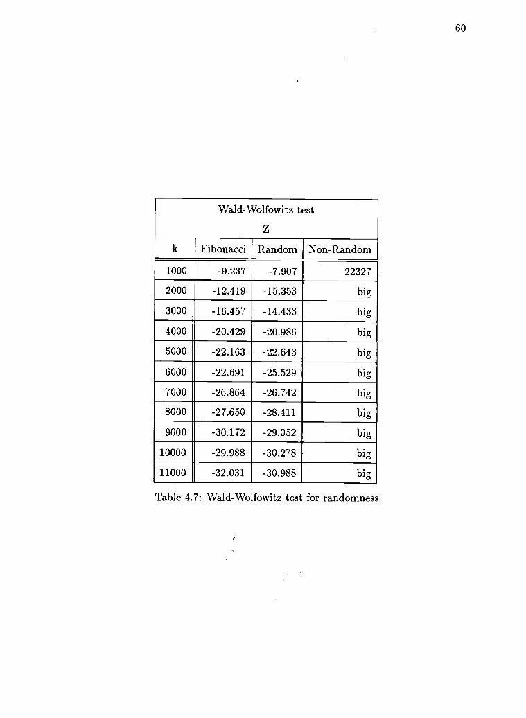
60
Wald-Wolfowitz test
Z
k Fibonacci Random Non-Random
1000 -9.237 -7.907 22327
2000 -12.419 -15.353 big
3000 -16.457 -14.433 big
4000 -20.429 -20.986 big
5000 -22.163 -22.643 big
6000 -22.691 -25.529 big
7000 -26.864 -26.742 big
8000 -27.650 -28.411 big
9000 -30.172 -29.052 big
10000 -29.988 -30.278 big
11000 -32.031 -30.988 big
Table 4.7: Wald-Wolfowitz test for randomness

61
not reject the hypothesis at the 99% level that the words are equally distributed.
The hypothesis can be rejected, that is, the words are not equally distributed, for
several entries in the table at the 99% level. The Fibonacci sequence when n =
1500 and n = 2500 and the random sequence when n = 1500, n = 3500, n = 4500,
and n = 5500.
4.2.2 Serial Test
Equal distribution is not enough to be reasonably sure that a sequence of numbers
is random. The sequence of numbers 1, 2, 3, 1, 2, 3, 1, 2, 3, is equally
distributed but not random. The serial test will measure the frequency of pairs of
numbers following one another. For each pair of numbers r1 and r2, 0 < r1, r2 < d
a count Cr1, of the number of occurrences of r1 immediately followed by r2 is kept
and should be evenly distributed over the d2 pairs of r1 and r2. To test the evenness
of the distribution, the chi-square test was applied with the probability of 17 for
each category. Similar tests can be conducted using triples or quadruples of numbers
instead of pairs, but the number of categories quickly becomes unmanageable.
Table 4.6 gives the value of x2/df for the number of occurrences of each pair
of words that appear in order. The number of words examined ranged from 300 to
3300 in increments of 300. Again, the hypothesis that the number of occurrences
of word pairs is equally distributed, can be rejected at the 99% level in only a few
entries of table 4.6. The hypothesis can be rejected in the Fibonacci column when
n = 2400 and in the random column when n = 1200 and n = 2400.
4.2.3 Wald-Wolfowitz Total Number of Runs Test
The Wald-Wolfowitz total number of runs test, [28], examines the grouping of similar
objects in the sequence. Let a run be defined as a consecutive group of characters
from the sequence,

62
such that 3k-1 sk, sk = sk+1 = = sk+n_2 and Sk+n_1 sk4.,. For
example, the bits 001111001 have four runs, two runs of zeros of length two each
and two runs of ones of lengths four and one. A random sequence of characters will
likely not have each character grouped together, Icor is it likely to have the character
perfectly shuffled, the Wald-Wolfowitz will meas...xe this grouping.
Table 4.7 gives the value of z for the Wald-Wolfowitz test with the number
of bits examined equal to n. The values for z indicate that the number of runs
is different than what we should expect if they were random. At the 99% level
the values should be between -2.326 and 2.326. The values of z for the Fibonacci
sequence of bits is similar to the values of z for the random sequence and different
from the non-random sequence, a sequence of all ones.
4.3 Cycles in the b Bit of fn
Let the sequence .tai be the sequence formed by concatenating the ith bit of fn for n
from 0 to oo. The bits to the left of the left most one bit of fn are assumed to be
zeros. If the ith bit of fn is examined independently of the the other bits a cycle is
apparent. For i = 0 the sequence Bo is
011011011011011...
Similar sequences appear for other i as well.
Theorem 4.1 The cycle length of the sequence Bn is 3 2n .
Proof. Since(
3.2n1 1 1 f3.2n-F1 1 1
1 0 fo = 0 f3 2n) if
1 0
3.2"
(1 0= I then f3.2n+1 mod 2n+1 = fl and f3.2n mod 2n+1 f0.
0 1
It will be shown that
3.2n
( 1 1
1 0mod 2n+1 =
( 1 0= I.
mod 271+1
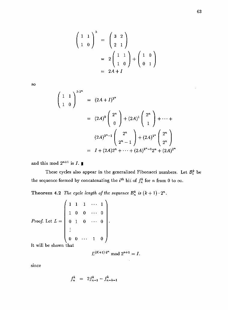
SO
1 0
3.2"
( 3 2
2 1
= 2 1 1 1 0
( 1 0 ) 0 1
2A + /
= (2A + /)2n
(2A)° 2) (2A)10
2n )1
(2A)2n-1 2n (2A)2n ( 2n )2n
= I + (2A)2n + + (2A)2n-12n (2A)2n
63
and this mod 27/44 is I. I
These cycles also appear in the generalized Fibonacci numbers. Let Blie be
the sequence formed by concatenating the ith bit of f! for n from 0 to oo.
Theorem 4.2 The cycle length of the sequence 13! is (k + 1) r.
1 1 1 1
1 0 0 0
Proof. Let L= 0 1 0 0
0 0 1 0
It will be shown that
since
L(K+1)2n mod 2n+1 = I.
fn = 2 k _

64
Ln
LnLn-k-1
Lk+1
(Lk+1)2n
2Ln-1 Ln-k-1
Ln-1 Ln-k-1= 2 Ln-k-1 Ln-k-1
= 2Lk I
= (2Lk I)2n
= (2Lk)° ( 2n ) (2e)1 ( 2n ) + +
(-1
2n(2Lk)2n
2n 1 )(2Lk)2n + + (2e)2n-1271 + (2.0)2n
and this mod 2n+1 is I. Therefore
/ \ (K1-1)2n1 1 1 1
1 0 0 0
0 1 0 0 mod 2n+1 =
0 0 1 0
If the entire cycle must be computed to find the nth element the cycle this
method will be useful only in computing the low order bits since the cycle lengths
grow exponentially with the bit position. If there were a way to directly compute
the nth bit of the cycle Bi we might be able to construct an algorithm to compute
fn using fewer bit operations than is currently known.
There are patterns in the Bi sequeneces, but they are not well understood
yet. The observations of these patterns is presented in the limited detail that they
are known. The patterns that are discussed break the cycle into six bit groups that
place one on top of the other with the least significant bit in the upper left corner
of the pile. Table 4.8 shows the bit patterns for 51,52, 83, 84, and 135 where j is
the jth group of six bits in the cycle.
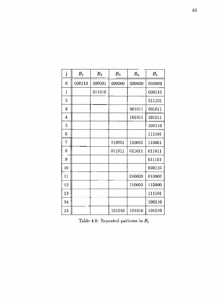
65
i B1 B2 83 B4 135
0 000110 000001 000000 000000 000000
1 011010 000110
2 011101
3 001011 001011
4 101011 101011
5 100110
6 111101
7 110001 110001 110001
8 011011 011011 011011
9 011101
10 000110
11 010000 010000
12 110000 110000
13 111101
14 100110
15 101010 101010 101010
Table 4.8: Repeated patterns in Bi

66
Let 8; (j) be the jth group of 6 bits of the sequence B. From table 4.8 it can
be seen that
and also
83(0) = 84(0) = 85(0) = 000000
83(1) = 84(3) = 85(7) = 110001
83(2) = 84(4) = 85(8) = 011011
83(3) = 84(7) = 85(15) = 101010
84(1) = 85(3) = 001011
84(2) = 85(4) = 101011
84(5) = 85(11) = 010000
84(6) = 135(12) = 110000
If this pattern continued then
but actually
86(0) = 85(0) 86(3) = 85(1) 86(4) = 85(2)
86(7) = 85(3) 86(8) = 85(4) 86(11) = 85(5)
136(12) = 85(6) 86(15) = 85(7) 86(13) = 85(8)
86(0) = 85(0) 86(4) = 85(1) 86(3) = 85(2)
86(8) = 85(3) 86(7) = 85(4) 86(12) = 85(5)
86(11) = 55(6) 86(16) = 135(7) 86(15) = 85(8)
The six bit segments 86(4 i 1) and 86(4 i) are switched in positions relative to
what was predicted from earlier observations for 1 < i < 7. When 87 was examined
it also exhibited the same patterns, including the switch, along with one higher level
67
switch. Presumably, 138 shows that same patterns as 137 with one further switch and
so on.
If this pattern of switching could be understood we would have a method of
computing the nth bit of 13, for each bit i in fn. This appears promising since the
cycle 13, can be entered, at most, six bits from the bit we want, and starting with
the low order bits we can use addition to compute those missing six bit positions.
This method could be applied iteratively to compute each bit in fn.
The incentive to investigate this method is that it appears that it may be
possible to compute the ith bit of fn in constant time. If this were the case we could
compute fn in linear time. This is still very speculative and unsuccessful to date.

68
Chapter 5
Conclusions and Future Research
This thesis has presented several algorithms for computing Fibonacci numbers. Ta-
ble 5.1 lists the algorithms and the number of bit operations the algorithm uses to
compute fn.
A few of the algorithms developed led naturally to computing fr, for any
positive n, but most algorithms more naturally compute fn for n = 2i. The fastest
algorithm for computing f, n = 2i, the product of factors algorithm, was used to
develope a fast algorithm to compute fn for any n.
The additive algorithms must add n numbers, each Arn bits long, using
about Ain2 bit operations. The multiplicative algorithms usually multiply q_ bit
numbers to compute the nth Fibonacci number using about, with our assumption
that multiplication uses n2 bit operations, (Arn)2 bit operations. Since Ar < 1 the
multiplicative algorithms will, when n is big enough, be faster than the additive
algorithms.
Several versions of the Ziv Lempel compression algorithm and dynamic Huff-
man code compression algorithm failed to compress the sequence of bits generated
by concatenating the binary representation of the Fibonacci numbers. The sequence
of bits behaved similarly to the random bits generated using the linear congruential
method in three tests of randomness.
Further research needs to be done on the patterns that appear in the bth bit
of fn. Understanding of these patters may lead to an in:7rovement in the order of
the number of bit operations used to compute fn. Another method of computing
the Fibonacci numbers that was not discussed here but may lead to a fast algorithm

69
Algorithm
Name
number of
bit-operations
fn for any n
or n = 2' section new
Natural Recursive Co(A7) any n 2.1 no
Repeated addition 0 (Ar (74 I)) any n 2.2 no
Binet's Formula 0 ((JVn + log n)2) n = 2' 2.3 no
Extending Vorob'ev 0 (i.nri 2) n = 2` 2.4 yes_ik 2 )
3 Multiply Matrix 0 ((.Ain)2) n = 2' 2.6.1 no
2 Multiply Matrix 0 (a nicLLi 2) n = 2' 2.6.2 yesk 3 fBinomial Coefficients 0(n3) any n 2.8 no
Product of Factors 0 ( .Au'.LLI.2) n = 2' 2.10 yesk 12 J
Product of Factors 0 (3(Arn)2) any n 2.10 yes
Gries and Levin f! 0 ( k2 (Ai n = 2' 2.5 nok nip)Generalized addition ./.4` 0 (Ar(n2 n)) any n 2.2 yes
Table 5.1: Summary of bit operation complexity using n2 multiply

70
is computing the number of nodes in a complete AVL tree. It might be possible
to recursively remove the top part of the AVL tree, the part that is a binary tree,
leaving several smaller AVL trees.
Finally, the applicability of these methods to computing f! and eventually
to more general recurrence relations should be investigated.
71
Bibliography
[1] Aho, A. V., J. E. Hoperoft and J. D. Ullman, "The Design and Analysis ofComputer Algorithms," Addison-Wesley, Reading MA; 1974.
[2] Anderson, P. G., "Fibonaccene," in Fibonacci Numbers and Their Applications,A. N. Philippou et al. (eds.), D. Reidel Publishing Company, Boston; 1986.
[3] Avriel, M. and D. J. Wilde, "Optimality proof for the symetric fibonacci searchtechnique," in Fibonacci Quarterly,4, 265-269; 1966.
[4] Beyer, W. H., Ed., "CRC Standard Mathematical Tables", 27th edition, CRCPress Inc, Boca Ratan FL; 1984.
[5] Bird, R. S., "Tabulation techniques for recursive programs," in ComputingSurveys,12, 403-413; 1980.
[6] Brousseau, A., "Relation of zeros to periods in the Fibonacci sequence moduloa prime," in American Math Monthly,71, 897-899; 1964.
[7] Brousseau, A., "Fibonacci and Related Number Theoretic tables," The Fi-bonacci Association, San Jose; 1972.
[8] Capocelli, R. M., and P. Cull, "Generalized Fibonacci numbers are roundedpowers," Technical report no. 87-50-1, Oregon State University, Departmentof Computer Science; 1987.
[9] Dickson, L. E., "History of the Theory of Numbers," Vol. 1, Carnegie Institu-tion of Washington, Washington D. C., 393 411; 1919.
[10] Er, M. C., "A fast algorithm for computing order-k Fibonacci numbers," inThe Computer Journal,26, 224-227; 1983.
[11] Er, M. C., "Computing sums of order-k Fibonacci numbers in log time," inInformation Processing Letters,17, 1-5; 1983.
[12] Fiduccia, C. M., "An efficient formula for linear recurrences," in SIAM Journalof Computing,14, 106-112; 1985.
[13] Gerald, C. F., and P. 0. Wheatley, "Applied Numberical Analysis," AddisonWesley, Reading MA; 1984.

72
[14] Goetgheluck, P., "Computing binomial coefficients," in American Math Monthly,94,360-365; 1987.
[15] Gries, D. and G. Levin, "Computing Fibonacci numbers (and similarly definedfunctions) in log time," in Information Processing Letters,11, 68-69; 1980.
[22]
[23]
[24]
[25]
Horowitz, E. and S. Sahni, "Fundamentals of Data Structures," Computerscience press, Rockville MD; 1982.
Jean, R. V., "Mathematical Approach to Pattern and Form in Plant Growth,"John Wiley and Sons, New York NY; 1984.
Kiefer, J., "Sequential minimax search for a maximum," in Procedings of theAmerican Math Society,4, 502-506; 1953.
Knuth, D. E., "The Art of Computer Programming," Vol.Reading MA; 1973.
Knuth, D. E., "The Art of Computer Programming," Vol.Reading MA; 1981.
1, Addison-Wesley,
2, Addison-Wesley,
Lahr, J., "Fibonacci and Lucas numbers and the Morgan-Voyce polynomials inladder networks and in electric line theory," in Fibonacci Numbers and TheirApplications, A. N. Philippou et al. (eds.), D. Reidel Publishing Company,Boston; 1986.
Lewis, T. G. and M. Z. Smith, "Applying Data Structures," Houghton Miff lin,Bostion; 1982.
Lynch, W. C., The t-Fibonacci numbers and polyphaseQuarter ly8, 6-22; 1970.
Oliver, L. T., and D. J. Wilde, "Symmetric sequentialmaximum," in Fibonacci Quarterly,2, 169-175; 1964.
sorting," in Fibonacci
minimax search for a
Pettorossi, A., "Derivation of an 0(k2 log n) algorithm for computing order-k Fibonacci numbers from the 0(1d log n) matrix multiplication method," inInformation Processing Letters, 11, 172-179; 1980.
[26] Pettorossi, A. and R. M. Burstall, "Deriving very efficient algorithms for evalu-atinb linear recurrence relations using the program transformation technique,"in Acta Infomatica,18, 181-206; 1982.
[27] Reingold, E. M. and W. J. Hansen, "Data Structures," Little, Brown andCompany; 1983.
[28] Romano, A., "Applied statistics for science and industry", Allyn and Bacon,Boston; 1977.

73
[29] Rosen, K. H., "Elementary Number Theory and Its Applications," pp 60-61,Addison Wesley, Reading MA; 1984.
[30] Rotkieicz, A., "Problems on the Fibonacci numbers and their generalizations,"in Fibonacci Numbers and Their Applications, A. N. Philippou et al. (eds.),D. Reidel Publishing Company; 1986.
[31] St. John, P. H., "On the asymptotic proportions of zeros and ones in Fibonaccisequences," in Fibonacci Quarterly, 22, 144-145; 1984.
[32] Shortt J., "An iterative program to calculate Fibonacci Numbers in O(logn)arithmetic operations," in Information Processing Letters,7, 299-303; 1977.
[33] Urbanek, F. J., "An O(log n) algorithm for computing the nth element of thesolution of a difference equation," in Information Processing Letters,11, 66-67;1980.
[34] Vinson J., "The relation of a period modulo to the rank of apparition of m inthe Fibonacci sequence," in Fibonacci Quarterly,2, 37-45; 1963.
[35] Vitter, J. S. "Design and analysis of dynamic Huffman codes," in Journal ofthe Association for Computing Machinery, 34, 825-845; 1987.
[36] Vorob'ev, N.N., "Fibonacci Numbers," Pergamon press, New York; 1961.
[37] Wall, D. D., "Fibonacci series modulo in," in American Math Monthly,67,525-532; 1960.
[38] Welch, T. A., "A technique for high-perfomance data compression," in Corn-puter,17, 8-19; 1984.
[39] Witten, I. H., R. M. Neal and J. G. Cleary, "Arithmetic coding for data com-pression," in Communications of the ACM,30, 520-540; 1987.
[40] Ziv, J. and A. Lempel, "On the complexity of finite sequences," in IEEE Trans-actions on Information Theory,IT-22, 75-81; 1976.
[41] Ziv, J. and A. Lempel, "A universal algorithm for sequential data compression,"in IEEE Transactions on Information Theory,IT-23, 337-343; 1977.
[42] Ziv, J. and A. Lempel, "Compression of individual sequences via variable-ratecoding," in IEEE Transactions on Information Theory, IT-24, 530-536; 1978.

Appendices

Appendix A
List of Fibonacci Relations
fn-I-2 = fn+1 fn n > 0, fo = 0, fl = 1
fn = 2f1:-1
fn = (i+ig I=2)= 1* (11;/g)n + 0.5i , n 0
( 1 ) fn -1
fn+i fn1 1
f2n-1-1 = +
fni-i(fn+i + 2fn) = f2n+2
fn(2fn+1 fn) = f2n
fn+k = fnifk + fnfk+i
f2n =
f2n+1 = fnifn+i + fn(fn +1 + fn)
G(z) = z/(1 z z2)
(.1:)2 2( -1)n =
f2i-Fk fk
Nn = log2 al =
151:1 = (k + 1) 2n
1.1
2.3
2.5
2.6
2.7
2.8
2.9
2.10
2.12
2.13
2.18
2.20
2.21
3.1
74

75
Appendix B
Lisp Functions
B.1 Natural Recursion
(defun rec-fib (n)
(cond ((= n 1) 1)
((= n 0) 0)
(t (+ (rec-fib (- n 1)) (rec-fib (- n 2))))))
B.2 Repeated Addition
(defun add-fib (n)
(cond ((eq n 1) 1)
((eq n 0) 0)
(t
(prog (previ prev2 next)
(setq previ 0)
(setq prev2 1)
(return (do ((i n (- i 1))) ((= i 1) prev2)
(setq next (+ previ prev2))
(setq previ prev2)
(setq prev2 next)))))))
B.3 Binet's Formula
(defun binet-fib-help (i)
(* (- (expt (/ (+ 1 sqrt5) 2) i)
(expt (/ (- 1 sqrt5) 2) i))
inverted_sqrt5))
(defun binet-fib (i)

76
(setq sqrt5 (my-sqrt 5 (/ 1 (ash 1 i)))) ; Get the i most significant
(setq inverted_sqrt5 (/ 1 sqrt5)) ; bits of \( sqrt{5} \)
(binet-fib-help i))
(defun fib (n)
(cond ((eql 4 n) 3)
(t (ceiling (* (square (fib (/ n 2))) (sqrt 5))))))
B.4 N. N. Vorob'ev's Methods
(defun nnv2-fib (i)
(cond ((= 0 i) 0)
((= 2 i) 1)
((oddp i) (add-fib i))
(t (- (square (nnv2-fib (+ (/ i 2) 1)))
(square (nnv2-fib (- (/ i 2) 1)))))))
(defun nnv3-fib (i)
(cond ((= 0 i) 0)
((not (= 0 (mod i 3))) (add-fib i))
(t (- (+ (expt (nnv3-fib (+ (/ i 3) 1)) 3)
(expt (nnv3-fib (/ i 3)) 3))
(expt (nnv3-fib (- (/ i 3) 1)) 3)))))
(defun nnv4-fib (i)
(cond ((eql i 1) '(1 (0 1)))
(t (let* ((fiba (nnv4-fib (/ i 2)))
(fibb (let* ((1st (cadr fiba))
(n (car 1st)
(np1 (cadr 1st))
(nm1 (- np1 n)))
(+ (* nml npl)
(* n
(+ np1 n))))))
(list (* (car fiba) (+ fibb (- fibb (car fiba))))
(list (car fiba) fibb))))))

77
B.5 Matrix Methods
B.5.1 Three Multiply Matrix Method
(defun mat-fib (i)
(cond ((eq 1 i) '((1 1) (1 0)))
(t (mat-square (mat-fib (/ i 2))))))
(defun mat-square (mat)
(prog (n+1 n n-1)
(setq n+1 (square (car (car mat))))
(setq n (square (car (car (cdr mat)))))
(setq n-1 (square (car (cdr (car (cdr mat))))))
(return (list (list (+ n+1 n) (setq temp (- n+1 n-1)))
(list temp (+ n n-1))))))
B.5.2 Two Multiply Matrix Method
(defun mat2-fib (i)
(cond ((eq 1 i) '((1 1) (1 0)))
(t (mat2-square (mat2-fib (ash i -1))))))
(defun mat2-square (mat)
(prog (alpha beta
(old-alpha (caar mat))
(old-beta (cadar mat)))
(setq alpha (* old-alpha
(+ old-alpha
(ash old-beta 1))))
(setq beta (* old-beta
(- (ash old-alpha 1)
old-beta)))
(return (list (list (setq temp (- alpha beta))
beta)
(list beta
(- temp beta))))))
B.6 Generating Function
(defun beta (i)
(cond ((eq 1 i) '(3))

78
(t (prog (temp)
(setq temp (beta (- i 1)))
(return (push (- (* (car temp) (car temp)) 2) temp))))))
(defun gf2-fib (i)
(cond ((= 0 i) 1)
((= 1 i) 1)
(t (apply '* (beta (- i 1))))))
(defun gf4-fib (n) (gf4-fib-help (round (log n 2))))
(defun gf4-fib-help (n m o)
(let ((b 3)
(limit (- n 1)))
(do ((i 1 (+ i 1))) ((>= i limit) m)
(setf b (- (* b b) 2))
(setf m (- (* m b) o)))))
(defun anyf (n)
(let ((a0 3) (s0 0)
(al 2) (sl 1)
(b 3)
(alpha0-list '(3 1)) (alphal-list '(2 1))
(limit (- (integer-length n) 1)))
(do ((i 2 (+ i 1))) ((>= i limit) t)
(setf b (- (* b b) 2))
(push (setf a0 (- (* a0 b) s0)) alpha0-list)
(push (setf al (- (* al b) sl)) alphal-list))
(anyf-help n
limit
(reverse alpha0-list)
(reverse alphal-list))))
(defun anyf-help (n q alpha0-list alphal-list)
(cond ((eql n 0) 0)
((eql n 1) 1)
((eql n 2) 1)
(t (+ (* (nth (- q 1) alphal-list)
(anyf-help (setf n (- n (ash 1 q)))
(- (integer-length n) 1)

79
alpha0-list
alphal- list))
(* (nth (- q 1) alpha0-list)
(anyf-help (incf n)
(- (integer-length n) 1)
alpha0-list
alphal-list))))))
B.7 Binomial Coefficients
(defun std2-binomial (n k)
(prog ((binom 1))
(return (do ((i n (- i 1)) (j k (- j 1))) ((= j 0) binom)
(setq binom (* (/ i j) binom))))))
(defun mult2-binomial (n k)
(cond ((= k 0) 1)
((= k 1) n)
(t (/ (apply '* (gen-values n (- n k)))
(apply '* (gen-values k 1))))))
B.8 Generalized Fibonacci Numbers
(defun kfib (n k)
(prog ((mem (append '(1 1) (make-list (- k 1) :initial-element '0)))
(limit (- n k)))
(return (do ((i 1 (+ i 1))) ((> i limit) (car mem))
(setq mem (nbutlast (nconc (list (- (ash (car mem) 1)
(car (last mem))))
mem)))))))
(defun gries-expo (mat n)
(do ((i 0 (+ i 1))) ((>= i n) mat)
(gries-square mat)))
(defun gries-square (mat)
(let ((new-bottom (vector-mat-mult (car mat) (cdr mat))))
(rplca mat new-bottom)
(mapcar #'(lambda (elem 1st)

80
(nsubstitute-if elem #'t 1st :count 1 :from-end t))
new-bottom
(cdr mat))))


![[Trading] Fibonacci Trader Gann Swing Chartist Dynamic Fibonacci Channels](https://img.pdfslide.us/doc/110x75/55cf9d87550346d033ae02c7/trading-fibonacci-trader-gann-swing-chartist-dynamic-fibonacci-channels.jpg)