1

2

Sorting Algorithms

- rearranging a list of numbers into increasing (strictly nondecreasing) order.

3

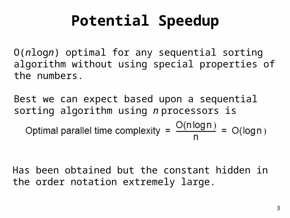
Potential Speedup

O(nlogn) optimal for any sequential sorting algorithm without using special properties of the numbers.

Best we can expect based upon a sequential sorting algorithm using n processors is

Has been obtained but the constant hidden in the order notation extremely large.

4

Compare-and-Exchange Sorting AlgorithmsCompare and Exchange

Form the basis of several, if not most, classical sequential sorting algorithms.

Two numbers, say A and B, are compared. If A > B, A and B are exchanged, i.e.:

if (A > B) {temp = A;A = B;B = temp;

}

5

Message-Passing Compare and Exchange

Version 1

P1 sends A to P2, which compares A and B and sends back B to P1 if A is larger than B (otherwise it sends back A to P1):

6

Alternative Message Passing Method

Version 2

For P1 to send A to P2 and P2 to send B to P1. Then both processes perform compare operations. P1 keeps the larger of A and B and P2 keeps the smaller of A and B:

7

Note on Precision of Duplicated Computations

Previous code assumes that the if condition, A > B, will return the same Boolean answer in both processors.

Different processors operating at different precision could conceivably produce different answers if real numbers are being compared.

This situation applies to anywhere computations are duplicated in different processors to reduce message passing, or to make the code SPMD.

8

Data Partitioning(Version 1)

p processors and n numbers. n/p numbers assigned to eachprocessor:

9

Merging Two Sublists — Version 2

10

Bubble Sort

First, largest number moved to the end of list by a series ofcompares and exchanges, starting at the opposite end.

Actions repeated with subsequent numbers, stopping just before the previously positioned number.

In this way, the larger numbers move (“bubble”) toward one end,

11

12

Time Complexity

Number of compare and exchange operations

Indicates a time complexity of O(n2) given that a single compare-and- exchange operation has a constant complexity, O(1).

13

Parallel Bubble SortIteration could start before previous iteration finished if does not overtake previous bubbling action:

14

Odd-Even (Transposition) Sort

Variation of bubble sort.

Operates in two alternating phases, even phase and odd phase.

Even phaseEven-numbered processes exchange numbers with their right neighbor.

Odd phaseOdd-numbered processes exchange numbers with their right neighbor.

15

Odd-Even Transposition SortSorting eight numbers

16

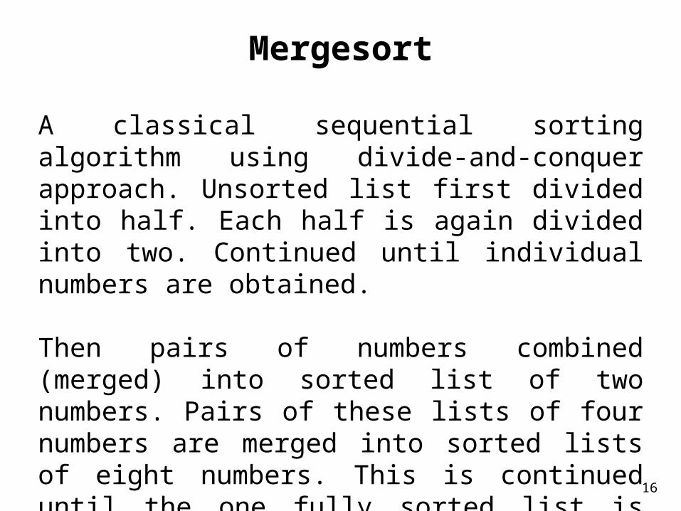
Mergesort

A classical sequential sorting algorithm using divide-and-conquer approach. Unsorted list first divided into half. Each half is again divided into two. Continued until individual numbers are obtained.

Then pairs of numbers combined (merged) into sorted list of two numbers. Pairs of these lists of four numbers are merged into sorted lists of eight numbers. This is continued until the one fully sorted list is obtained.

17

Parallelizing MergesortUsing tree allocation of processes

18

Analysis

Sequential

Sequential time complexity is O(nlogn).

Parallel

2 log n steps in the parallel version but each step may need to perform more than one basic operation, depending upon the number of numbers being processed - see text.

19

QuicksortVery popular sequential sorting algorithm that performs well with average sequential time complexity of O(nlogn).

First list divided into two sublists. All numbers in one sublist arranged to be smaller than all numbers in other sublist.

Achieved by first selecting one number, called a pivot, against which every other number is compared. If the number is less than the pivot, it is placed in one sublist. Otherwise, it is placed in the other sublist.

Pivot could be any number in the list, but often first number in list chosen. Pivot itself could be placed in one sublist, or the pivot could be separated and placed in its final position.

20

Parallelizing Quicksort

Using tree allocation of processes

21

With the pivot being withheld in processes:

22

Analysis

Fundamental problem with all tree constructions – initial division done by a single processor, which will seriously limit speed.

Tree in quicksort will not, in general, be perfectly balanced Pivot selection very important to make quicksort operate fast.

23

Work Pool Implementation of Quicksort

First, work pool holds initial unsorted list. Given to first processor which divides list into two parts. One part returned to work pool to be given to another processor, while the other part operated upon again.

24

Neither Mergesort nor Quicksort parallelize very well as theprocessor efficiency is low (see book for analysis).

Quicksort also can be very unbalanced. Can use load balancing techniques.

25

Batcher’s Parallel Sorting Algorithms

• Odd-even Mergesort

• Bitonic Mergesort

Originally derived in terms of switching networks.

Both are well balanced and have parallel time complexity of O(log2n) with n processors.

26

Odd-Even Mergesort

Odd-Even Merge Algorithm

Start with odd-even merge algorithm which will merge two sorted lists into one sorted list. Given two sorted lists a1, a2, a3, …, an and b1, b2, b3, …, bn (where n is a power of 2).

27

Odd-Even Merging of Two Sorted Lists

28

Odd-Even MergesortApply odd-even merging recursively

29

Bitonic MergesortBitonic Sequence

A monotonic increasing sequence is a sequence of increasing numbers.

A bitonic sequence has two sequences, one increasing and one decreasing. e.g.

a0 < a1 < a2, a3, …, ai-1 < ai > ai+1, …, an-2 > an-1

for some value of i (0 <= i < n).

A sequence is also bitonic if the preceding can be achieved by shifting the numbers cyclically (left or right).

30

Bitonic Sequences

31

“Special” Characteristic of Bitonic Sequences

If we perform a compare-and-exchange operation on ai with ai+n/2 for all i, where there are n numbers in the sequence, get TWO bitonic sequences, where the numbers in one sequence are all less than the numbers in the other sequence.

32

Creating two bitonic sequences from one bitonic sequence

Starting with the bitonic sequence

3, 5, 8, 9, 7, 4, 2, 1we get:

33

Sorting a bitonic sequence

Compare-and-exchange moves smaller numbers of each pair to left and larger numbers of pair to right. Given a bitonic sequence, recursively performing operations will sort the list.

34

SortingTo sort an unordered sequence, sequences are merged into larger bitonic sequences, starting with pairs of adjacent numbers.

By a compare-and-exchange operation, pairs of adjacent numbers formed into increasing sequences and decreasing sequences. Pairs form a bitonic sequence of twice size of each original sequences.

By repeating this process, bitonic sequences of larger and larger lengths obtained.

In the final step, a single bitonic sequence sorted into a single increasing sequence.

35

Bitonic Mergesort

36

37

Phases

The six steps (for eight numbers) are divided into three phases:

Phase 1 (Step 1) Convert pairs of numbers into increasing/decreasing sequences and into 4-bitbitonic sequences.

Phase 2 (Steps 2/3) Split each 4-bit bitonic sequence into two 2-bit bitonic sequences, highersequences at center.Sort each 4-bit bitonic sequence

increasing/ decreasing sequences and merge into 8-bit bitonic sequence.

Phase 3 (Steps 4/5/6)Sort 8-bit bitonic sequence.

38

Number of Steps

In general, with n = 2k, there are k phases, each of 1, 2, 3, …, k steps. Hence the total number of steps is given by

39

Sorting Conclusions so far

Computational time complexity using n processors

• Odd-even transposition sort - O(n)

• Parallel mergesort - O(n) but unbalanced processor load and Communication

• Parallel quicksort - O(n) but unbalanced processor load, and communication can generate to O(n2)

• Odd-even Mergesort and Bitonic Mergesort O(log2n)

Bitonic mergesort has been a popular choice for a parallel sorting.

40

Sorting on Specific NetworksAlgorithms can take advantage of the underlying interconnection network of the parallel computer.

Two network structures have received specific attention: the mesh and hypercube because parallel computers have been built with these networks.

Of less interest nowadays because underlying architecture often hidden from user - We will describe a couple of representative algorithms.

MPI features for mapping algorithms onto meshes, and one can always use a mesh or hypercube algorithm even if the underlying architecture is not the same.

41

Mesh - Two-Dimensional SortingThe layout of a sorted sequence on a mesh could be row by row or snakelike. Snakelike:

42

ShearsortAlternate row and column sorting until list fully sorted. Row sortingalternative directions to get snake-like sorting:

43

Shearsort

44

Using Transposition

Causes the elements in each column to be in positions in a row.Can be placed between the row operations and column operations

45

Hypercube

Quicksort

Hypercube network has structural characteristics that offer scope for implementing efficient divide-and-conquer sorting algorithms, such as quicksort.

46

Complete List Placed in One Processor

Suppose a list of n numbers placed on one node of a d-dimensional hypercube.

List can be divided into two parts according to the quicksort algorithm by using a pivot determined by the processor, with one part sent to the adjacent node in the highest dimension.

Then the two nodes can repeat the process.

47

Example3-dimensional hypercube with the numbers originally in node 000:

Finally, the parts sorted using a sequential algorithm, all in parallel. If required, sorted parts can be returned to one processor in a sequence that allows processor to concatenate sorted lists to create final sorted list.

48

Hypercube quicksort algorithm- numbers originally in node 000

49

There are other hypercube quicksort algorithms - see textbook.

50

Other Sorting Algorithms

We began by giving the lower bound for the time complexity of a sequential sorting algorithm based upon comparisons as O(nlogn).

Consequently, the time complexity of a parallel sorting algorithm based upon comparisons is O((logn)/p) with p processors or O(logn) with n processors.

There are sorting algorithms that can achieve better than O(nlogn) sequential time complexity and are very attractive candidates for parallelization but they often assume special properties of the numbers being sorted.

51

Rank Sort as basis of a parallel sorting algorithm

Does not achieve a sequential time of O(nlogn), but can be parallelized easily, and leads us onto linear sequential time algorithms which can be parallelized to achieve O(logn) parallel time and are attractive algorithms for clusters.

52

Rank SortNumber of numbers that are smaller than each selected

number counted. This count provides the position of selected number in sorted list; that is, its “rank.”

• First a[0] is read and compared with each of the other numbers, a[1] … a[n-1], recording the number of numbers less than a[0].

• Suppose this number is x. This is the index of the location in the final sorted list.

• The number a[0] is copied into the final sorted list b[0] … b[n-1], at location b[x]. Actions repeated with the other numbers.

Overall sequential sorting time complexity of O(n2) (not exactly a good sequential sorting algorithm!).

53

Sequential Code

for (i = 0; i < n; i++) { /* for each number */x = 0;for (j = 0; j < n; j++) /* count number less

than it */if (a[i] > a[j]) x++;

b[x] = a[i]; /* copy number into correct place */}

This code will fail if duplicates exist in the sequence of numbers. Easy to fix. (How?)

54

Parallel CodeUsing n Processors

One processor allocated to each number. Finds final index in O(n) steps. With all processors operating in parallel, parallel time complexity O(n).

In forall notation, the code would look like

forall (i = 0; i < n; i++) { /* for each no in parallel*/ x = 0; for (j = 0; j < n; j++) /* count number less than it */

if (a[i] > a[j]) x++; b[x] = a[i]; /* copy no into correct place */}

Parallel time complexity, O(n), as good as any sorting algorithm so far. Can do even better if we have more processors.

55

Using n2 Processors

Comparing one number with the other numbers in list using multiple processors:

n - 1 processors used to find rank of one number. With n numbers, (n - 1)n processors or (almost) n2 processors needed. Incrementing counter done sequentially and requires maximum of n steps. Total number of steps = 1 + n.

56

Parallel Rank Sort Conclusions

Easy to do as each number can be considered in isolation.

Rank sort can sort in:

O(n) with n processorsor

O(logn) using n2 processors.

In practical applications, using n2 processors prohibitive.

Theoretically possible to reduce time complexity to O(1) byconsidering all increment operations as happening in parallel since they are independent of each other.

57

Message Passing Parallel Rank SortMaster-Slave Approach

Requires shared access to list of numbers. Master process responds to request for numbers from slaves. Algorithm better for shared memory

58

Counting Sort

If the numbers to be sorted are integers, there is a way of coding the rank sort algorithm to reduce the sequential time complexity from O(n2) to O(n), called as Counting Sort.

As in the rank sort code suppose the unsorted numbers stored in an array a[] and final sorted sequence is stored in array b[]. Algorithm uses an additional array, say c[], having one element for each possible value of the numbers. Suppose the range of integers is from 1 to m. The array has element c[1] through c[m] inclusive. Now, let us working through the algorithm in stages.

59

Stable Sort Algorithms

Algorithms that will place identical numbers in the same order as in the original sequence.

Counting sort is naturally a stable sorting algorithm.

60

First, c[ ] will be used to hold the histogram of the sequence, that is, the number of each number. This can be computed in O(m) time with code such as:

for (i = 1; i <= m; i++)c[i] = 0;

for (i = 1; i <= m; i++)c[a[i]]++;

61

Next stage: The number of numbers less than each number found by performing a prefix sum operation on array c[ ].

In the prefix sum calculation, given a list of numbers, x0, …, xn-1, all the partial summations (i.e., x0; x0 + x1; x0 + x1 + x2; x0 + x1 + x2 + x3; … ) are computed.

Here, the prefix sum is computed using the histogram originally held in c[ ] in O(m) time as described below:

for (i = 2; i <= m; i++)c[i] = c[i] + c[i-1];

62

Final stage: The numbers are placed in the sorted order in O(n) time as described below:

for (i = n; i >= 1; i--) {b[c[a[i]]] = a[i]c[a[i]]--; /* ensures stable sorting */

}

Complete code has O(n + m) sequential time complexity. If m is linearly related to n as it is in some applications, the code has O(n) sequential time complexity.

63

Counting sort

64

Parallelizing counting sort can use the parallel version of the prefix sum calculation which requires O(logn) time with n - 1 processors.

The final sorting stage can be achieved in O(n/p) time with p processors or O(1) with n processors by simply having the body of the loop done by different processors.

65

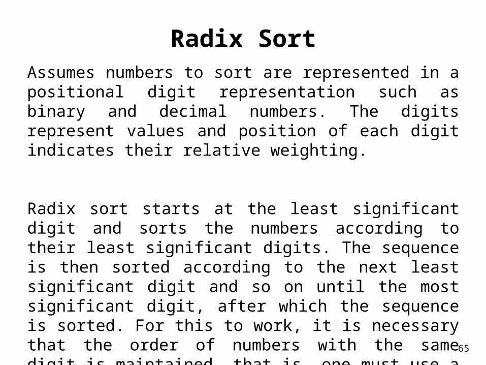
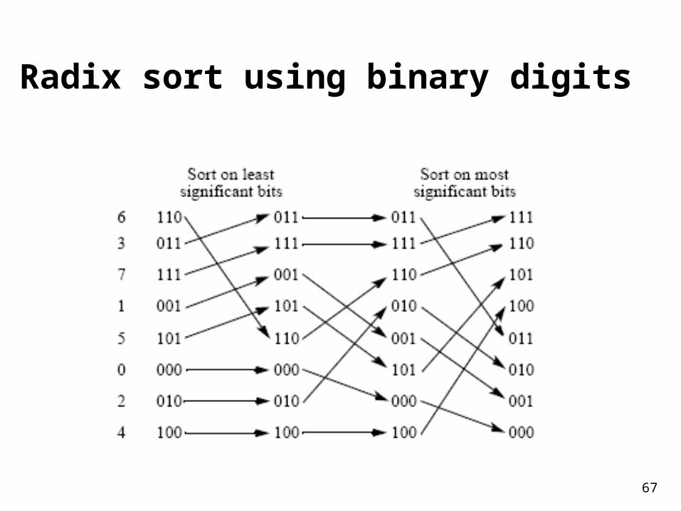
Radix SortAssumes numbers to sort are represented in a positional digit representation such as binary and decimal numbers. The digits represent values and position of each digit indicates their relative weighting.

Radix sort starts at the least significant digit and sorts the numbers according to their least significant digits. The sequence is then sorted according to the next least significant digit and so on until the most significant digit, after which the sequence is sorted. For this to work, it is necessary that the order of numbers with the same digit is maintained, that is, one must use a stable sorting algorithm.

66

Radix sort using decimal digits

67

Radix sort using binary digits

68

Radix sort can be parallelized by using a parallel sorting algorithm in each phase of sorting on bits or groups of bits.

Already mentioned parallelized counting sort using prefix sum calculation, which leads to O(logn) time with n - 1 processors and constant b and r.

69

Example of parallelizing radix sort sorting on binary digits

Can use prefix-sum calculation for positioning each number at each stage. When prefix sum calculation applied to a column of bits, it gives number of 1’s up to each digit position because all digits can only be 0 or 1 and prefix calculation will simply add number of 1’s.A second prefix calculation can also give the number of 0’s up to each digit position by performing the prefix calculation on the digits inverted (diminished prefix sum).When digit considered being a 0, diminished prefix sum calculation provides new position for number.When digit considered being a 1, result of normal prefix sum calculation plus largest diminished prefix calculation gives final position for number.

70

Sample Sort

Sample sort is an old idea (pre1970) as are many basic sorting ideas. Has been discussed in the context of quicksort and bucket sort.

In context of quicksort, sample sort takes a sample of s numbers from the sequence of n numbers. The median of this sample is used as the first pivot to divide the sequence into two parts as required as the first step by the quicksort algorithm rather than the usual first number in the list.

71

In context of bucket sort, objective of sample sort is to divide theranges so that each bucket will have approximately the same number of numbers.

Does this by using a sampling scheme which picks out numbers from the sequence of n numbers as splitters which define the range of numbers for each bucket. If there are m buckets, m - 1 splitters are needed.

Can be found by the following method. The numbers to be sorted are first divided into n/m groups. Each group is sorted and a sample of s equally spaced numbers are chosen from each group. This creates ms samples in total which are then sorted and m - 1 equally spaced numbers selected as splitters.

72

Selecting splitters - Sample sort version of bucket sort

73

Sorting Algorithms on ClustersFactors for efficient implementation on clusters:

Using collective operations such broadcast, gather, scatter, and reduce provided in message-passing software such as MPI rather than non-uniform communication patterns that require point-to-point communication, because collective operations expected to be implemented efficiently.

Distributed memory of a cluster does not favor algorithms requiring access to widely separately numbers. Algorithms that require only local operations are better, although all sorting algorithms finally have to move numbers in the worst case from one end of sequence to other somehow.

74

Cache memory -- better to have an algorithm that operate upon a block of numbers that can be placed in the cache. Will need to know the size and organization of the cache, and this has to become part of thealgorithm as parameters.

Clusters of SMP processors (SMP clusters) -- algorithms need to take into account that the groups of processors in each SMP system may operate in the shared memory mode where the shared memory is only within each SMP system, whereas each system may communicate with other SMP systems in the cluster in a message-passing mode. Again to take this into account requires parameters such as number of processors within each SMP system and size of the memory in each SMP system.