Chapter 1 A Light Introduction to Modelling Recurrent

Chapter 1

A Light Introduction to ModellingRecurrent Epidemics

David J.D. Earn

Abstract Epidemics of many infectious diseases occur periodically. Why?

1.1 Introduction

There are many excellent books that provide broad and deep introductionsto the mathematical theory of infectious disease epidemics, ranging frommonographs and textbooks [1–7] to collections of articles from workshopsand conferences [8–12]. My goal in this article is to spark an interest inmathematical epidemiology that might inspire you to dig into the existingliterature (starting with the rest of this book [13]) and, perhaps, to engagein some research yourself in this fascinating area of science.

I will discuss some famous epidemics that present challenging theoreticalquestions, and – without getting bogged down in technical details you canfind elsewhere – I will try to convince you that you can fairly easily buildand analyze simple models that help us understand the complex patternsevident in these data. Not wishing to give you a false impression of the field,I will also briefly mention some epidemic patterns that do not appear to beexplicable in terms of simple models (at least, not in terms of simple modelswe have thought of!).

Several of the following sections are based in part on an even lighter intro-duction to the subject of mathematical epidemiology that I wrote for a highschool mathematics magazine [14]. Here, I do not limit myself to high schoolmathematics, but I hope the bulk of the article will be easily accessible toyou if you have had an elementary course in ordinary differential equations.

Department of Mathematics and StatisticsMcMaster University, Hamilton, ON, Canada L8S [email protected]

3

4 D.J.D. Earn

1.2 Plague

One of the most famous examples of an epidemic of an infectious disease in ahuman population is the Great Plague of London, which took place in 1665–1666. We know quite a lot about the progression of the Great Plague becauseweekly bills of mortality from that time have been retained. A photographof such a bill is shown in Fig. 1.1. Note that the report indicates that thenumber of deaths from plague (5,533) was more than 37 times the numberof births (146) in the week in question, and that wasn’t the worst week! (Aneven worse plague occurred in the fourteenth century, but no detailed recordsof that epidemic are available.)

Putting together the weekly counts of plague deaths from all the relevantmortality bills, we can obtain the epidemic curve for the Great Plague, whichI’ve plotted in the top left panel of Fig. 1.2. The characteristic exponentialrise, turnover and decline is precisely the pattern predicted by the classicsusceptible-infective-recovered (SIR) model of Kermack and McKendrick [15]that I describe below. While this encourages us to think that mathematicalmodelling can help us understand epidemics, some detailed features of theepidemic curve are not predicted by the simple SIR model. For example,the model does not explain the jagged features in the plotted curve (andthere would be many more small ups and downs if we had a record of dailyrather than weekly deaths). However, with some considerable mathematicaleffort, these “fine details” can be accounted for by replacing the differentialequations of Kermack and McKendrick with equations that include stochas-tic (i.e., random) processes [2]. We can then congratulate ourselves for ourmodelling success. . . until we look at more data.

The bottom left panel of Fig. 1.2 shows weekly mortality from plague inLondon over a period of 70 years. The Great Plague is the rightmost (andhighest) peak in the plot. You can see that on a longer timescale, there was acomplex pattern of plague epidemics including extinctions and re-emergences.This cannot be explained by the basic SIR model (even if we reformulate itusing stochastic processes). The trouble is likely that we have left out a keybiological fact: there is a reservoir of plague in rodents, so it can persist foryears, unnoticed by humans, and then re-emerge suddenly and explosively. Byincluding the rodents and aspects of spatial spread in a mathematical model,it has recently been possible to make sense of the pattern of seventeenthcentury plague epidemics in London [16]. Nevertheless, some debate continuesas to whether all those plagues were really caused by the same pathogenicorganism.

1 Modelling Recurrent Epidemics 5

Fig. 1.1 A bill of mortality for the city of London, England, for the week of 26 Septemberto 3 October 1665. This photograph was taken by Claire Lees at the Guildhall in London,England, with the permission of the librarian

1.3 Measles

A less contentious example is given by epidemics of measles, which are def-initely caused by a well-known virus that infects the respiratory tract inhumans and is transmitted by airborne particles [3]. Measles gives rise tocharacteristic red spots that are easily identifiable by physicians who haveseen many cases, and parents are very likely to take their children to a doctorwhen such spots are noticed. Consequently, the majority of measles cases in

6 D.J.D. Earn

Fig. 1.2 Epidemic curves for plague in London (left panels) and measles in New YorkCity (right panels). For plague, the curves show the number of deaths reported each week.For measles, the curves show the number of cases reported each month. In the top panels,the small ticks on the time axis occur at monthly intervals

developed countries end up in the office of a doctor (who, in many countries,is required to report observed measles cases to a central body). The result isthat the quality of reported measles case data is unusually good, and it hastherefore stimulated a lot of work in mathematical modelling of epidemics.

An epidemic curve for measles in New York City in 1962 is shown in thetop right panel of Fig. 1.2. The period shown is 17 months, exactly the samelength of time shown for the Great Plague of London in the top left panel. The1962 measles epidemic in New York took off more slowly and lasted longerthan the Great Plague of 1665. Can mathematical models help us understandwhat might have caused these differences?

1.4 The SIR Model

Most epidemic models are based on dividing the host population (humans inthe case of this article) into a small number of compartments, each containing


individuals that are identical in terms of their status with respect to thedisease in question. In the SIR model, there are three compartments:

• Susceptible: individuals who have no immunity to the infectious agent, somight become infected if exposed

• Infectious: individuals who are currently infected and can transmit theinfection to susceptible individuals who they contact

• Removed : individuals who are immune to the infection, and consequentlydo not affect the transmission dynamics in any way when they contactother individuals

It is traditional to denote the number of individuals in each of these com-partments as S, I and R, respectively. The total host population size isN = S + I + R.

Having compartmentalized the host population, we now need a set of equa-tions that specify how the sizes of the compartments change over time. Solu-tions of these equations will yield, in particular, I(t), the size of the infectiouscompartment at time t. A plot of I(t) should bear a strong resemblance toobserved epidemic curves if this is a reasonable model.

The numbers of individuals in each compartment must be integers, ofcourse, but if the host population size N is sufficiently large we can treat S,I and R as continuous variables and express our model for how they changein terms of a system of differential equations,

dS

dt= −βSI , (1.1a)

dI

dt= βSI − γI . (1.1b)

Here, the transmission rate (per capita) is β and the recovery rate is γ (sothe mean infectious period is 1/γ). Note that I have not written a differentialequation for the number of removed individuals. The appropriate equation isdR/dt = γI (outflow from the I compartment goes into the R compartment)but since R does not appear in (1.1a) and (1.1b) the equation for dR/dthas no effect on the dynamics of S and I (formalizing the fact that removedindividuals cannot affect transmission). This basic SIR model has a longhistory [15] and is now so standard that you can even find it discussed insome introductory calculus textbooks [17].

If everyone is initially susceptible (S(0) = N), then a newly introducedinfected individual can be expected to infect other people at the rate βNduring the expected infectious period 1/γ. Thus, this first infective individualcan be expected to infect R0 = βN/γ individuals. The number R0 is calledthe basic reproduction number and is unquestionably the most importantquantity to consider when analyzing any epidemic model for an infectiousdisease. In particular, R0 determines whether an epidemic can occur at all;to see this for the basic SIR model, note in (1.1a) and (1.1b) that I can neverincrease unless R0 > 1. This makes intuitive sense, since if each individual

8 D.J.D. Earn

transmits the infection to an average of less than one individual then thenumber of cases must decrease with time.

So, how do we obtain I(t) from the SIR model?

1.5 Solving the Basic SIR Equations

If we take the ratio of (1.1a) and (1.1b) we obtain

dI

dS= −1 +

1R0S

, (1.2)

which we can integrate immediately to find

I = I(0) + S(0) − S +1

R0ln [S/S(0)] . (1.3)

This is an exact solution, but it gives I as a function of S, not as a functionof t. Plots of I(S) for various R0 show the phase portraits of solutions(Fig. 1.3) but do not give any indication of the time taken to reach any par-ticular points on the curves. While the exact expression for the phase portraitmay seem like great progress, it is unfortunately not possible to obtain anexact expression for I(t), even for this extremely simple model.

In their landmark 1927 paper, Kermack and McKendrick [15] found anapproximate solution for I(t) in the basic SIR model, but their approximationis valid only at the very beginning of an epidemic (or for all time if R0 isunrealistically close to unity) so it would not appear to be of much use forunderstanding measles, which certainly has R0 > 10.

Computers come to our rescue. Rather than seeking an explicit formulafor I(t) we can instead obtain an accurate numerical approximation of thesolution. There are many ways to do this [18], but I will briefly mentionthe simplest approach (Euler’s method), which you can implement in a fewminutes in any standard programming language, or even a spreadsheet.

Over a sufficiently small time interval ∆t, we can make the approximationdS/dt � ∆S/∆t, where ∆S = S(t+∆t)−S(t). If we now solve for the numberof susceptibles a time ∆t in the future, we obtain

S(t + ∆t) = S(t) − βS(t)I(t)∆t . (1.4a)

Similarly, we can approximate the number of infectives at time t + ∆t as

I(t + ∆t) = I(t) + βS(t)I(t)∆t − γI(t)∆t . (1.4b)

Equations (1.4a) and (1.4b) together provide a scheme for approximatingsolutions of the basic SIR model. To implement this scheme on a computer,you need to decide on a suitable small time step ∆t. If you want to try


Fig. 1.3 Phase portraits of solutions of the basic SIR model ((1.1a) and (1.1b)) for a newlyinvading infectious disease. The curves are labelled by the value of the basic reproductionnumber R0 (2, 4, 8 or 16). For each curve, the initial time is at the bottom right cornerof the graph (I(0) � 0, S(0) � N). All solutions end on the S axis (I → 0 as t → ∞).A simple analytical formula for the phase portrait is easily derived (1.3); from this it iseasy to show that limt→∞ S(t) > 0 regardless of the value of R0 (though, as is clear fromthe phase portraits plotted for R0 = 8 and 16, nearly everyone is likely to be infectedeventually if R0 is high)

this, I suggest taking ∆t to be one tenth of a day. I should point out thatI am being extremely cavalier in suggesting the above method. Do try this,but be forewarned that you can easily generate garbage using this simpleapproach if you’re not careful. (To avoid potential confusion, include a linein your program that checks that S(t) ≥ 0 and I(t) ≥ 0 at all times. Anotherimportant check is to repeat your calculations using a much smaller ∆t andmake sure your results don’t change.)

In order for your computer to carry out the calculations specified by (1.4a)and (1.4b), you need to tell it the parameter values (β and γ, or R0, N andγ) and initial conditions (S(0) and I(0)). For measles, estimates that areindependent of the case report data that we’re trying to explain indicate thatthe mean infectious period is 1/γ ∼ 5 days and the basic reproduction numberis R0 ∼ 18 [3]. The population of New York City in 1960 was N = 7, 781, 984.

10 D.J.D. Earn

If we now assume one infectious individual came to New York before theepidemic of 1962 (I(0) = 1), and that everyone in the city was susceptible(S(0) = N), then we have enough information to let the computer calculateI(t). Doing so yields the epidemic curve shown in the top panel of Fig. 1.4,which does not look much like the real data for the 1962 epidemic in NewYork. So is there something wrong with our model?

Fig. 1.4 Epidemic curves for measles in New York City, generated by the basic SIR model.The curves show the number of infectives I(t) at time t. In the top two panels, the small tickson the time axis occur at monthly intervals. The parameter values and initial conditions arediscussed in the main text, except for the initial proportion susceptible used to generatethe bottom two panels (S(0)/N = 0.065). This initial condition was determined basedon the SIR model with vital dynamics, as specified by (1.5a) and (1.5b). The proportionsusceptible at equilibrium is S = 1/R0 = 1/18 � 0.056. At the start of each epidemic cyclethat occurs as the system approaches the equilibrium, the proportion susceptible must behigher than S

No, but there is something very wrong with our initial conditions. Thebottom right panel of Fig. 1.2 shows reported measles cases in New YorkCity for a 36-year period, the end of which includes the 1962 epidemic. Evi-dently, measles epidemics had been occurring in New York for decades with nosign of extinction of the virus. In late 1961, most of New York’s population


had already had measles and was already immune, and the epidemic cer-tainly didn’t start because one infectious individual came to the city. Theassumptions that I(0) = 1 and S(0) = N are ridiculous. If, instead, wetake I(0) = 123 ∗ (5/30) (the number of reported cases in September 1961times the infectious period as a proportion of the length of the month) andS(0) = 0.065 ∗ N , then we obtain the epidemic curve plotted in the middlepanel of Fig. 1.4, which is much more like the observed epidemic curve ofFig. 1.2 (top right panel).

This is progress – we have a model that can explain a single measlesepidemic in New York City – but the model cannot explain the recurrentepidemics observed in the bottom right panel of Fig. 1.2. This is not becausewe still don’t have exactly the right parameter values and initial conditions:no parameter values or initial conditions lead to recurrent epidemics in thissimple model. So, it would seem, there must be some essential biologicalmechanism that we have not included in our model. What might that be?

Let’s think about why a second epidemic cannot occur in the model we’vediscussed so far. The characteristic turnover and decline of an epidemic curveoccurs because the pathogen is running out of susceptible individuals to in-fect. To stimulate a second epidemic, there must be a source of susceptibleindividuals. For measles, that source cannot be previously infected people,because recovered individuals retain lifelong immunity to the virus. So whois it?

Newborns. They typically acquire immunity from their mothers, but thiswanes after a few months. A constant stream of births can provide the sourcewe’re looking for.

1.6 SIR with Vital Dynamics

If we expand the SIR model to include B births per unit time and a naturalmortality rate µ (per capita) then our equations become

dS

dt= B − βSI − µS , (1.5a)

dI

dt= βSI − γI − µI . (1.5b)

The timescale for substantial changes in birth rates (decades) is generallymuch longer than a measles epidemic (a few months), so we’ll assume thatthe population size is constant (thus B = µN , so there is really only one newparameter in the above equations and we can take it to be B). As before,we can use Euler’s trick to convert the equations above into a scheme thatenables a computer to generate approximate solutions. An example is shownin the bottom panel of Fig. 1.4, where I have taken the birth rate to beB = 126, 372 per year (the number of births in New York City in 1928, the

12 D.J.D. Earn

first year for which we have data). The rest of the parameters and initialconditions are as in the middle panel of the figure.

Again we seem to be making progress. We are now getting recurrent epi-demics, but the oscillations in the numbers of cases over time damp out, even-tually reaching an equilibrium (S, I). Of course, the bottom plot in Fig. 1.4shows what happens for only one set of possible initial conditions. Perhaps fordifferent initial conditions the oscillations don’t damp out? If you try a dif-ferent set of initial conditions – or lots of different sets of initial conditions –then I guarantee that you will see the same behaviour. The system will alwaysundergo damped oscillations and converge to (S, I). How can I be so sure,you might ask?

First of all, by setting the derivatives in (1.5a) and (1.5b) to zero, you caneasily calculate (in terms of the model’s parameters) expressions for S and Ithat are positive (hence meaningful) provided R0 > 1. Then, by linearizing(1.5a) and (1.5b) about the equilibrium and computing the eigenvalues of theJacobian matrix for the system, you will find that the equilibrium is locallystable (the eigenvalues have negative real parts) and approach to the equi-librium is oscillatory (the eigenvalues have non-zero imaginary parts) [3, 7].But maybe if we are far enough from the equilibrium undamped oscillationsare possible?

No, we can prove rigorously that the equilibrium (S, I) is globally asymp-totically stable, i.e., all initial conditions with S(0) > 0 and I(0) > 0 yieldsolutions that converge onto this equilibrium. One way to see this is to scalethe variables by population size (S → S/N , I → I/N) and consider thefunction

V (S, I) = S − S log S + I − I log I , S, I ∈ (0, 1). (1.6)

With a little work you can show that the time derivative of V along solutionsof the model, i.e., ∇V ·(dS/dt, dI/dt) with dS/dt and dI/dt taken from (1.1a)and (1.1b), is strictly negative for each S, I ∈ (0, 1). V is therefore a Lyapunovfunction [19] for the basic SIR model. The existence of such a V ensures theglobal asymptotic stability of the equilibrium (S, I) [19].

Finding a Lyapunov function is generally not straightforward, but func-tions similar the one given in (1.6) have recently been used to prove global sta-bility of equilibria in many epidemic models [20]. The upshot for our presentattempt to understand measles dynamics is that this rigorous argument al-lows us to rule out the basic SIR model: it cannot explain the real oscillationsin measles incidence in New York City from 1928 to 1964, which showed noevidence of damping out. Back to the drawing board?


1.7 Demographic Stochasticity

One thing we have glossed over is the presence of noise. While it is truethat for sufficiently large population size N it is reasonable to treat S andI as continuous variables, it is not true that the true discreteness of thenumber of individuals in each compartment has no observable effect. Thiswas recognized by Bartlett [1] who found that a relatively small amount ofnoise was sufficient to prevent the oscillations of the basic SIR model fromdamping out. Whether we recast the SIR model as a stochastic process [2,21]or simply add a small noise term to the deterministic equations, we cansustain the oscillations that damp out in the bottom panel of Fig. 1.4.

Again, this is progress that has arisen from an important mechanisticinsight. But we are left with another puzzle. If you look carefully at the NewYork City measles reports in the bottom right panel of Fig. 1.2 you’ll see thatbefore about 1945 the epidemics were fairly irregular, whereas after 1945they followed an almost perfect 2-year cycle. Even with oscillations sustainedby noise, the SIR model cannot explain why the measles epidemic patternin New York City changed in this way. Have we missed another importantmechanism?

1.8 Seasonal Forcing

So far, we have been assuming implicitly that the transmission rate β (or,equivalently, the basic reproduction number R0) is simply a constant and,in particular, that it does not change in time. Let’s think about that as-sumption. The transmission rate is really the product of the rate of contactamong individuals and the probability that a susceptible individual who iscontacted by an infectious individual will become infected. But the contactrate is not constant throughout the year. To see that, consider the fact thatin the absence of vaccination the average age at which a person is infectedwith measles is about 5 years [3], hence most susceptibles are children. Chil-dren are in closer contact when school is in session, so the transmission ratemust vary seasonally.

A crude approximation of this seasonality is to assume that β varies sinu-soidally,

β(t) = β0(1 + α cos 2πt) . (1.7)

Here, β0 is the mean transmission rate, α is the amplitude of seasonal varia-tion and time t is assumed to be measured in years. If, as above, β is assumedto be a periodic function (with period 1 year) then the SIR model is said tobe seasonally forced. We can still use Euler’s trick to solve the equations ap-proximately, and I encourage you to do that using a computer for variousvalues of the seasonal amplitude α (0 ≤ α ≤ 1).

14 D.J.D. Earn

You might think that seasonal forcing is just a minor tweak of the model.In fact, this forcing has an enormous impact on the epidemic dynamics thatthe model predicts. If you’ve ever studied the forced pendulum then youmight already have some intuition for this. A pendulum with some frictionwill exhibit damped oscillations and settle down to an equilibrium. But ifyou tap the pendulum with a hammer periodically then it will never settledown and it can exhibit quite an exotic range of behaviours including chaoticdynamics [22,23] (oscillations that look random). Similarly complex dynamicscan occur in the seasonally forced SIR model.

Importantly, with seasonal forcing the SIR model displays undamped os-cillations (and it does this, incidentally, even in the absence of stochasticity).More than that, for different parameter values, the seasonally forced SIRmodel can produce all the different types of oscillatory measles patterns Ihave ever seen in real data. So are we done?

No. As noted in the previous section, the observed measles epidemics inNew York City show very clearly that the dynamical pattern changed overtime (bottom right panel of Fig. 1.2) and other significant qualitative changeshave been observed in measles case series in other places [24]. How can weexplain changes over time in the pattern of measles epidemics?

1.9 Slow Changes in Susceptible Recruitment

Once again, the missing ingredient in the model is a changing parametervalue. This time it is the birth rate B, which is not really constant. Birthrates fluctuate seasonally, but to such a small extent that this effect is negli-gible. What turns out to be more important is the much slower changes thatoccur in the average birth rate over decades. For example, in New York Citythe birth rate was much lower during the 1930s (the “Great Depression”)than after 1945 (the “baby boom”) and this difference accounts for the verydifferent patterns of measles epidemics in New York City during these twotime periods [24].

A little more analysis of the SIR model is very useful. Intuitively, reduc-ing the birth rate or increasing the proportion of children vaccinated bothaffect the rate at which new susceptible individuals are recruited into thepopulation. In fact, it is possible to prove that changes in the birth rate haveexactly the same effect on disease dynamics as changes of the same relativemagnitude in the transmission rate or the proportion of the population thatis vaccinated [24]. This equivalence makes it possible to explain historicalcase report data for a variety of infectious diseases in many different cities.

Interestingly, it turns out that while most aspects of the dynamics ofmeasles can be explained by employing seasonal forcing without noise, bothseasonal forcing and stochasticity are essential to explain the dynamics ofother childhood diseases [25].


1.10 Not the Whole Story

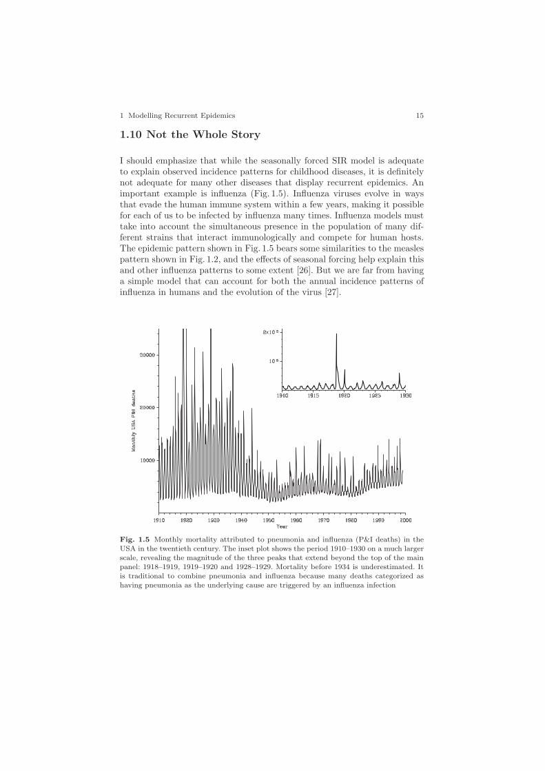
I should emphasize that while the seasonally forced SIR model is adequateto explain observed incidence patterns for childhood diseases, it is definitelynot adequate for many other diseases that display recurrent epidemics. Animportant example is influenza (Fig. 1.5). Influenza viruses evolve in waysthat evade the human immune system within a few years, making it possiblefor each of us to be infected by influenza many times. Influenza models musttake into account the simultaneous presence in the population of many dif-ferent strains that interact immunologically and compete for human hosts.The epidemic pattern shown in Fig. 1.5 bears some similarities to the measlespattern shown in Fig. 1.2, and the effects of seasonal forcing help explain thisand other influenza patterns to some extent [26]. But we are far from havinga simple model that can account for both the annual incidence patterns ofinfluenza in humans and the evolution of the virus [27].

Fig. 1.5 Monthly mortality attributed to pneumonia and influenza (P&I deaths) in theUSA in the twentieth century. The inset plot shows the period 1910–1930 on a much largerscale, revealing the magnitude of the three peaks that extend beyond the top of the mainpanel: 1918–1919, 1919–1920 and 1928–1929. Mortality before 1934 is underestimated. Itis traditional to combine pneumonia and influenza because many deaths categorized ashaving pneumonia as the underlying cause are triggered by an influenza infection

16 D.J.D. Earn

1.11 Take Home Message

One thing that you may have picked up from this article is that successfulmathematical modelling of biological systems tends to proceed in steps. Webegin with the simplest sensible model and try to discover everything we canabout it. If the simplest model cannot explain the phenomenon we’re tryingto understand then we add more biological detail to the model, and it’s bestto do this in steps because we are then more likely to be able to determinewhich biological features have the greatest impact on the behaviour of themodel.

In the particular case of mathematical epidemiology, we are lucky thatmedical and public health personnel have painstakingly conducted surveil-lance of infectious diseases for centuries. This has created an enormous wealthof valuable data [28] with which to test hypotheses about disease spread usingmathematical models, making this a very exciting subject for research.

Acknowledgements

It is a pleasure to thank Sigal Balshine, Will Guest and Fred Brauer forhelpful comments. The weekly plague data plotted in Fig. 1.2 were digitizedby Seth Earn.

References

1. M. S. Bartlett. Stochastic population models in ecology and epidemiology, volume 4of Methuen’s Monographs on Applied Probability and Statistics. Spottiswoode,Ballantyne, London, 1960.

2. N. T. J. Bailey. The Mathematical Theory of Infectious Diseases and Its Applications.Hafner, New York, second edition, 1975.

3. R. M. Anderson and R. M. May. Infectious Diseases of Humans: Dynamics and Con-trol. Oxford University Press, Oxford, 1991.

4. D. J. Daley and J. Gani. Epidemic modelling, an introduction, volume 15 ofCambridge: Studies in Mathematical Biology. Cambridge university press, Cambridge,1999.

5. H. Andersson and T. Britton. Stochastic epidemic models and their statistical analysis,volume 151 of Lecture Notes in Statistics. Springer, New York, 2000.

6. O. Diekmann and J. A. P. Heesterbeek. Mathematical epidemiology of infectious dis-eases: model building, analysis and interpretation. Wiley Series in Mathematical andComputational Biology. Wiley, New York, 2000.

7. F. Brauer and C. Castillo-Chavez. Mathematical models in population biology andepidemiology, volume 40 of Texts in Applied Mathematics. Springer, New York, 2001.

8. D. Mollison, editor. Epidemic Models: Their Structure and Relation to Data. Publi-cations of the Newton Institute. Cambridge University Press, Cambridge, 1995.

9. V. Isham and G. Medley, editors. Models for Infectious Human Diseases: Their Struc-ture and Relation to Data. Publications of the Newton Institute. Cambridge UniversityPress, Cambridge, 1996.


10. B. T. Grenfell and A. P. Dobson, editors. Ecology of Infectious Diseases in Natu-ral Populations. Publications of the Newton Institute. Cambridge University Press,Cambridge, 1995.

11. C. Castillo-Chavez, with S. Blower, P. van den Driessche, D. Kirschner, and A-A.Yakubu, editors. Mathematical approaches for emerging and reemerging infectiousdiseases: an introduction, volume 125 of The IMA Volumes in Mathematics and ItsApplications. Springer, New York, 2002.

12. C. Castillo-Chavez, with S. Blower, P. van den Driessche, D. Kirschner, and A-A.Yakubu, editors. Mathematical approaches for emerging and reemerging infectious dis-eases: models, methods and theory, volume 126 of The IMA Volumes in Mathematicsand Its Applications. Springer, New York, 2002.

13. F. Brauer, P. van den Driessche and J. Wu, editors. Mathematical Epidemiology (thisvolume).

14. D. J. D. Earn. Mathematical modelling of recurrent epidemics. Pi in the Sky, 8:14–17,2004.

15. W. O. Kermack and A. G. McKendrick. A contribution to the mathematical theory ofepidemics. Proceedings of the Royal Society of London Series A, 115:700–721, 1927.

16. M. J. Keeling and C. A. Gilligan. Metapopulation dynamics of bubonic plague. Nature,407:903–906, 2000.

17. D. Hughes-Hallett, A. M. Gleason, P. F. Lock, D. E. Flath, S. P. Gordon, D. O. Lomen,D. Lovelock, W. G. McCallum, B. G. Osgood, D. Quinney, A. Pasquale, K. Rhea,J. Tecosky-Feldman, J. B. Thrash, and T. W. Tucker. Applied Calculus. Wiley,Toronto, second edition, 2002.

18. W. H. Press, S. A. Teukolsky, W. T. Vetterling, and B. P. Flannery. Numerical Recipesin C. Cambridge University Press, Cambridge, second edition, 1992.

19. S. Wiggins. Introduction to applied nonlinear dynamical systems and chaos, volume 2of Texts in Applied Mathematics. Springer, New York, 2 edition, 2003.

20. A. Korobeinikov and P. K. Maini. A Lyapunov function and global properties for SIRand SEIR epidemiological models with nonlinear incidence. Mathematical Biosciencesand Engineering, 1(1):57–60, 2004.

21. D. T. Gillespie. A general method for numerically simulating the stochastic time evo-lution of coupled chemical reactions. Journal of Computational Physics, 22:403–434,1976.

22. J. Gleick. Chaos. Abacus, London, 1987.23. S. H. Strogatz. Nonlinear Dynamics and Chaos. Addison Wesley, New York, 1994.24. D. J. D. Earn, P. Rohani, B. M. Bolker, and B. T. Grenfell. A simple model for

complex dynamical transitions in epidemics. Science, 287(5453):667–670, 2000.25. C. T. Bauch and D. J. D. Earn. Transients and attractors in epidemics. Proceedings

of the Royal Society of London Series B-Biological Sciences, 270(1524):1573–1578,2003.

26. J. Dushoff, J. B. Plotkin, S. A. Levin, and D. J. D. Earn. Dynamical resonance canaccount for seasonality of influenza epidemics. Proceedings of the National Academyof Sciences of the United States of America, 101(48):16915–16916, 2004.

27. D. J. D. Earn, J. Dushoff, and S. A. Levin. Ecology and evolution of the flu. Trendsin Ecology and Evolution, 17(7):334–340, 2002.

28. IIDDA. The International Infectious Disease Data Archive, http://iidda.

mcmaster.ca.

Documents

Chapter 1 A Light Introduction to Modelling Recurrent