MEASURING AND MODELLING FORWARD LIGHT SCATTERING IN …

MEASURING AND

MODELLING FORWARD

LIGHT SCATTERING IN

THE HUMAN EYE

A thesis submitted to

The University of Manchester,

for the degree of Doctor of Philosophy,

in the Faculty of Life Sciences.

2015

Pablo Benito López

Optometry

2

THESIS CONTENT

THESIS CONTENT ...................................................................................................................... 2

LIST OF FIGURES ....................................................................................................................... 5

LIST OF TABLES ........................................................................................................................ 10

LIST OF EQUATIONS ............................................................................................................... 11

ABBREVIATIONS LIST ........................................................................................................... 12

ABSTRACT ................................................................................................................................... 13

DECLARATION .......................................................................................................................... 14

THESIS FORMAT ....................................................................................................................... 14

COPYRIGHT STATEMENT .................................................................................................... 15

ACKNOWLEDGEMENTS ....................................................................................................... 16

1. INTRODUCTION ................................................................................................................ 17

1.1 OVERVIEW .......................................................................................................... 17

1.2 WHAT IS INTRAOCULAR LIGHT SCATTER? ................................................ 18

1.3 INTRAOCULAR SCATTER, GLARE AND STRAYLIGHT.............................. 22

1.4 INTRAOCULAR SCATTER AND CONTRAST SENSITIVITY ....................... 23

1.5 SCATTER AND POINT SPREAD FUNCTION .................................................. 24

1.6 SOURCES OF SCATTER ..................................................................................... 26

1.6.1 CORNEA ....................................................................................................... 27

1.6.2 CRYSTALLINE LENS .................................................................................. 29

1.6.3 IRIS, SCLERA AND UVEAL TRACT ......................................................... 32

1.6.4 RETINA ......................................................................................................... 33

1.7 FACTORS AFFECTING INTRAOCULAR LIGHT SCATTER .......................... 33

1.7.1 PHYSIOLOGICAL ........................................................................................ 34

1.7.2 PATHOLOGICAL .......................................................................................... 34

1.7.3 OPTICAL ....................................................................................................... 39

1.8 METHODS TO MEASURE INTRAOCULAR LIGHT SCATTER .................... 40

1.8.1 METHODS BASED ON THE MEASUREMENT OF CONTRAST

SENTITIVITY .............................................................................................................. 40

1.8.2 METHODS BASED ON THE EQUIVALENT LUMINANCE TECHNIQUE

……………………………………………………………………………...42

1.8.3 ESTIMATIONS OF FORWARD LIGHT SCATTER FROM BACKWARD

LIGHT SCATTER ........................................................................................................ 49

3

1.8.4 METHODS BASED ON THE DOUBLE-PASS TECHNIQUE ................... 49

1.9 RATIONALE ......................................................................................................... 57

2. COMPARISON OF THE COMPENSATION COMPARISON METHOD AND

THE DIRECT COMPENSATION METHOD FOR STRAYLIGHT

MEASUREMENT ........................................................................................................................ 60

2.1 CONTRIBUTIONS .................................................................................................... 60

2.2 PUBLISHING OF THE PAPER ................................................................................ 60

2.3 PRESENTATION AT CONFERENCE ...................................................................... 60

2.4 ABSTRACT ............................................................................................................... 61

2.5 INTRODUCTION ...................................................................................................... 62

2.6 METHODS ................................................................................................................. 63

2.7 RESULTS ................................................................................................................... 67

2.8 DISCUSSION ............................................................................................................ 75

3. COMPARISON OF FORWARD LIGHT SCATTER ESTIMATIONS USING

HARTMANN - SHACK SPOT PATTERNS AND C-QUANT .......................................... 78

3.1 CONTRIBUTIONS .................................................................................................... 78



3.4 ABSTRACT ............................................................................................................... 79

3.5 INTRODUCTION ...................................................................................................... 80

3.6 METHODS ................................................................................................................. 82

3.7 RESULTS ................................................................................................................... 91

3.8 DISCUSSION ............................................................................................................ 93

4. FORWARD AND BACKWARD LIGHT SCATTER MEASUREMENTS IN THE

HUMAN EYE................................................................................................................................ 97

4.1 CONTRIBUTIONS .................................................................................................... 97



4.4 ABSTRACT ............................................................................................................... 98

4.5 INTRODUCTION ...................................................................................................... 98

4.6 METHODS ............................................................................................................... 101

4.7 RESULTS ................................................................................................................. 107

4.8 DISCUSSION .......................................................................................................... 110

5. INSTRUMENT AND COMPUTERIZED BASED MODEL FOR THE

OBJECTIVE MEASUREMENT OF FORWARD LIGHT SCATTER ......................... 115

4

5.1 CONTRIBUTIONS .................................................................................................. 115

5.2 PUBLISHING OF THE PAPER .............................................................................. 115

5.3 PRESENTATION AT CONFERENCE .................................................................... 115

5.4 ABSTRACT ............................................................................................................. 116

5.5 INTRODUCTION .................................................................................................... 117

5.6 REVIEW OF FLS MEASURING AND MODELING ............................................ 118

5.6.1 MODELLING FLS ............................................................................................ 118

5.6.2 MEASURING FLS ............................................................................................ 120

5.7 METHODS ............................................................................................................... 122

5.7.1 EXPERIMENTAL SET-UP USED FOR EXPERIMENT 1 AND 2 ................. 123

5.7.2 FIRST EXPERIMENT: VALIDATION OF THE PROTOTYPE WITH

CUSTOMISED LENSES AND ZEMAX MODEL ................................................... 126

5.7.3 SECOND EXPERIMENT: RESULTS FROM PARTICIPANTS, COMPARISON

RESULTS PROTOTYPE / C-QUANT AND PROTOTYPE / ZEMAX SCATTER

EYE MODEL ............................................................................................................. 128

5.8 RESULTS ................................................................................................................. 133




RESULTS PROTOTYPE / C-QUANT AND PROTOTYPE / ZEMAX SCATTER

EYE MODEL ............................................................................................................. 136

5.9 DISCUSSION .......................................................................................................... 139




RESULTS PROTOTYPE – C-QUANT AND PROTOTYPE / ZEMAX SCATTER

EYE MODEL ............................................................................................................. 139

6. FINAL SUMMARY AND FUTURE WORK ............................................................... 144

6.1 FINAL SUMMARY ................................................................................................. 144

6.2 FUTURE WORK ..................................................................................................... 145

7. REFERENCES ................................................................................................................... 147

ANNEXUS ................................................................................................................................... 169

Program to analyse the HS spot patterns ........................................................................ 169

5

LIST OF FIGURES

Figure 1.1: Types of scatter produced by different sizes of particles: Scatter produced by

small particles whose size is less than 1/10 the size of the incident wavelength) is

principally Rayleigh (A) and produces a homogenous scatter pattern around the particle.

For larger particles than the incident wavelength Mie scatter takes place (B and C). The

Mie scatter pattern produced by large particles is narrower in forward direction when the

particle is larger (C). ........................................................................................................... 19

Figure 1.2: Scatter light produced by large (A) and small particles (B). Large particles

scatter light giving a narrower pattern than small ones. Signal intensity from small

particles is however smaller than for large particles. ......................................................... 21

Figure 1.3: Retinal PSF from a point light source. A shows the image from that point in

ideal conditions while B shows the image from that point considering aberrations,

diffraction and scatter. ......................................................................................................... 24

Figure 1.4: Relationship between PSF (Log (PSF)) and the scatter angle Ө (in degrees)

obtained for a subject using a double pass system (Ginis et al., 2012). As it can be seen on

the figure, Log(PSF) becomes smaller as the measured scatter angle increases. ............... 25

Figure 1.5: Light scatter structures of the human eye. Major light scatter structures are the

cornea (30% of the incident light), crystalline lens (40%) and the retina (20%). Light

scatter through the iris in light pigmented eyes and through the sclera can be up to 5% of

the incident light. .................................................................................................................. 26

Figure 1.6: Structure of the cornea depicted from the epithelial to the endothelial layer

(epithelial layer, Bowman´s layer, stoma, Descemet´s membrane and endothelial layer).

Stroma is composed of regularly separated fibrils. Anatomically, both fibrils and

keratocytes are parallel to the different layers of the cornea, but have been depicted

perpendicularly for illustration purposes. ........................................................................... 28

Figure 1.7: Structure of the crystalline lens. The crystalline lens is internally composed of

a matrix of fibers which are equally distributed and surrounded by the cytoplasm. Cells

from the cytoplasm can migrate to different areas of the crystalline lens and create large

molecules that produce light scatter. .................................................................................... 30

Figure 1.8: The van den Berg straylight meter: The instrument is composed of 3 peripheral

annulus acting as glare sources and a central disc. The instrument gives the possibility of

measuring straylight at 3.5, 10 and 28 degrees of eccentricity with respect to the eye,

depending on the glare source that is used. The glare source has a flickering frequency of

8Hz and uses a wavelength of 570 ± 30nm. ......................................................................... 44

Figure 1.9: The scatter function from the City University Program (Chisholm, 2003). ..... 45

Figure 1.10: C-Quant stimulus screen. The instrument has a glare source with angle of 5

to 10 degrees with respect to the eye (7 degrees of effective scatter angle). The flickering

6

frequency of the glare source is 8Hz. The instrument uses an achromatic light. The test

field is composed of a circle with two half discs. ................................................................. 47

Figure 1.11: Double pass system. Basically, a double pass system is an optical instrument

where the light passes through the eye twice: light goes inside the eye to the retina and

from the retina back to the imaging system. The image created is called double pass image

(DP image). To develop a double pass system, a beam splitter is normally used. This beam

splitter can reflect and refract the incident light at same time. ........................................... 50

Figure 1.12: Estimations of intraocular scatter calculated as the difference between MTFs

from a DP image and HS (see below) systems (Pinero et al., 2010). .................................. 52

Figure 1.13: HS wavefront sensor detector. A HS detector is composed of an array of

microlenses that analyse an incident wavefront by focusing the light passing through each

one of the microlenses on a HS image. In case of an optically perfect eye, a plane

wavefront projected into the eye would leave the eye (after a double pass) still being a

plane wavefront. However, diffraction, aberrations and intraocular scatter in the eye will

modify the pattern of an incident plane wavefront to a distorted wavefront (after the double

pass). Incident plane wavefronts create HS images with clear dots while distorted

wavefronts create HS images with dots and a distribution on light around those dots as a

consequence of diffraction, aberrations and light scatter. ................................................... 53

Figure 1.14: A typical spot pattern of a HS image with spot pattern and the

neighbourhoods. ................................................................................................................... 54

Figure 1.15: Instrument for the reconstruction of the wide angle PSF in the human eye

(Ginis et al., 2013). In the figure, C is a condenser lens, D is diffuser, P is linear polarizers,

D1 and D2 diaphragms, LCWS is a liquid crystal selectable bandwidth tunable optical

filter, LC-SLM is a liquid crystal modulator and BS a beam splitter. .................................. 57

Figure 2.1: Van den Berg straylight meter and C-Quant straylight meter. The van den Berg

straylight meter has three different glare sources to measure at 3.5, 10 and 28 degrees of

eccentricity while the C-Quant straylight meter has only one at 7⁰ of effective eccentricity.

Glare sources in both instruments have a flickering frequency of 8Hz. In the van den Berg

straylight meter the testing field is a central disc while C-Quant has a circle with two

testing halves. C-Quant straylight meter uses a achromatic light while van den Berg

straylight meter uses LEDs of 570±30nm. ........................................................................... 65

Figure 2.2: Boxplot diagram representing the distribution of data for C-Quant and the

three Straylight meter eccentricities measured (S, M and L). Boxes contain 50% of the data

(from lower to upper quartile) while the line inside represents the median value. Vertical

lines cover from the minimum to the maximum value, excluding the outside values (circles)

and the far out values (black squares). ................................................................................ 68

Figure 2.3: Scatter value from C-Quant is plotted against the three different tested

eccentricities (S = 3.5⁰, M = 10⁰, L = 28⁰) of the Straylight meter (A = Straylight meter(S)

and C-Quant, B = Straylight meter (M) and C-Quant, C = Straylight meter for L is plotted

against the mean CQ). Pearson´s correlation coefficient and p value are shown on the

7

graphs. A weak relationship can be observed between values obtained from both

instruments. .......................................................................................................................... 70

Figure 2.4: The graphs show the differencies of the measurements between the two

methods plotted against their mean values for each one of the three different tested

eccentricities (A: S=3.5⁰, B: M=10⁰, C: L=28⁰). Mean value of the differences and limits

of agreement (defined as mean of the differences ± 1.96xSD) are also presented. .............. 72









consequence of diffraction, aberrations and light scatter. ................................................... 83

Figure 3.2: A) Hartmanngram spot pattern from one of the participants. In this picture,

each square represents an area of 13x13 pixels around the centroid; squares containing

more than two saturated points or whose intensity pixels were under the threshold

(obtained to analyse the images with Matlab) were not considered for calculations and

look missing. For this particular hartmanngram, the mean, standard deviation, minimum

and maximum of the standard deviations of all PSFlets were respectively 8.9x10-3

, 6.87x10-

2, 7.7x10

-3, 0.17. The associated HS value is equal to the maximum standard deviation. B)

An enlarged PSFlet showing the centre of the PSF and the surrounding intensity. The

sampling distance in the pupil plane is 0.23mm. ................................................................. 85

Figure 3.3: Photos of one 9mm RPG contact lens (left) for each density of aerosol droplets

(simulating different scatter conditions). Right: photo of the central zone of the lens (60%

of the lens = 38.06mm2) after processing with Matlab to assess objectively the droplets

density. First line of photos shows the non-sprayed lens. Consecutive lines correspond to

same lens with added quantities of spray (without removing the previous spraying). Pixel

size of the photos (obtained with a normal camera) is 1.4 microns and the mean droplet’s

size was 31.2 ± 21.52 pixels. ................................................................................................ 88

Figure 3.4: Relationship between the amount of FLS for each lens (extracted from the

hartmanngrams) and the associated concentration of scatter droplets. .............................. 91

Figure 3.5: Relationship between the FLS values obtained from the HS (abscissae) and

those from the C-Quant (ordinate). ...................................................................................... 92

Figure 4.1: Scheimpflug image obtained with Pentacam. Peak corneal densitometry value

is the highest intensity pixel obtained from a histogram of the cornea for a certain

measured meridian (top right corner, in green). 3D corneal densitometry assessment

divides the cornea in concentrical zones around the pupil centre and provides with an

average density value for each zone. The optical axis is represented with the dotted red

line. ..................................................................................................................................... 104

8

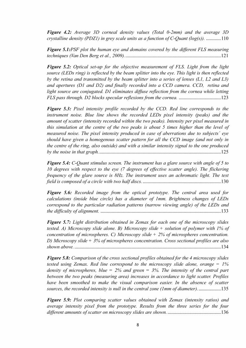
Figure 4.2: Average 3D corneal density values (Total 0-2mm) and the average 3D

crystalline density (PDZ1) in grey scale units as a function of C-Quant (log(s)). ............ 110

Figure 5.1:PSF plot the human eye and domains covered by the different FLS measuring

techniques (Van Den Berg et al., 2009). ............................................................................. 121

Figure 5.2: Optical set-up for the objective measurement of FLS. Light from the light

source (LEDs ring) is reflected by the beam splitter into the eye. This light is then reflected

by the retina and transmitted by the beam splitter into a series of lenses (L1, L2 and L3)

and apertures (D1 and D2) and finally recorded into a CCD camera. CCD, retina and

light source are conjugated. D1 eliminates diffuse reflection from the cornea while letting

FLS pass through. D2 blocks specular reflexions from the cornea. .................................. 123

Figure 5.3: Pixel intensity profile recorded by the CCD. Red line corresponds to the

instrument noise. Blue line shows the recorded LEDs pixel intensity (peaks) and the

amount of scatter (intensity recorded within the two peaks). Intensity per pixel measured in

this simulation at the centre of the two peaks is about 5 times higher than the level of

measured noise. The pixel intensity produced in case of aberrations due to subjects´ eye

should have given a homogenous scatter pattern for all the CCD image (and not only in

the centre of the ring, also outside) and with a similar intensity signal to the one produced

by the noise in that graph. .................................................................................................. 125

Figure 5.4: C-Quant stimulus screen. The instrument has a glare source with angle of 5 to

10 degrees with respect to the eye (7 degrees of effective scatter angle). The flickering


field is composed of a circle with two half discs. ............................................................... 130

Figure 5.6: Recorded image from the optical prototype. The central area used for

calculations (inside blue circle) has a diameter of 1mm. Brightness changes of LEDs

correspond to the particular radiation patterns (narrow viewing angle) of the LEDs and

the difficulty of alignment. ................................................................................................. 133

Figure 5.7: Light distribution obtained in Zemax for each one of the microscopy slides

tested. A) Microscopy slide alone. B) Microscopy slide + solution of polymer with 1% of

concentration of microspheres. C) Microscopy slide + 2% of microspheres concentration.

D) Microscopy slide + 3% of microspheres concentration. Cross sectional profiles are also

shown above. ...................................................................................................................... 134

Figure 5.8: Comparison of the cross sectional profiles obtained for the 4 microscopy slides

tested using Zemax. Red line correspond to the microscopy slide alone, orange = 1%

density of microspheres, blue = 2% and green = 3%. The intensity of the central part

between the two peaks (measuring area) increases in accordance to light scatter. Profiles

have been smoothed to make the visual comparison easier. In the absence of scatter

sources, the recorded intensity is null in the central zone (1mm of diameter). .................. 135

Figure 5.9: Plot comparing scatter values obtained with Zemax (intensity ratios) and

average intensity pixel from the prototype. Results from the three series for the four

different amounts of scatter on microscopy slides are shown. ........................................... 136

9

Figure 5.10: Image of the LEDs ring. Light distribution over the image is a consequence

of FLS. With FLS, the amount of light participating to the LEDs image decreases and the

amount of light at the centre of the ring increases. Green circle marks the area used for

calculations. ....................................................................................................................... 137

Figure 5.11: Comparison of the scatter values measured with the optical prototype (at

50cm distance at an angular eccentricity of 2.04 degrees. A good relationship was

obtained. ............................................................................................................................. 138

10

LIST OF TABLES

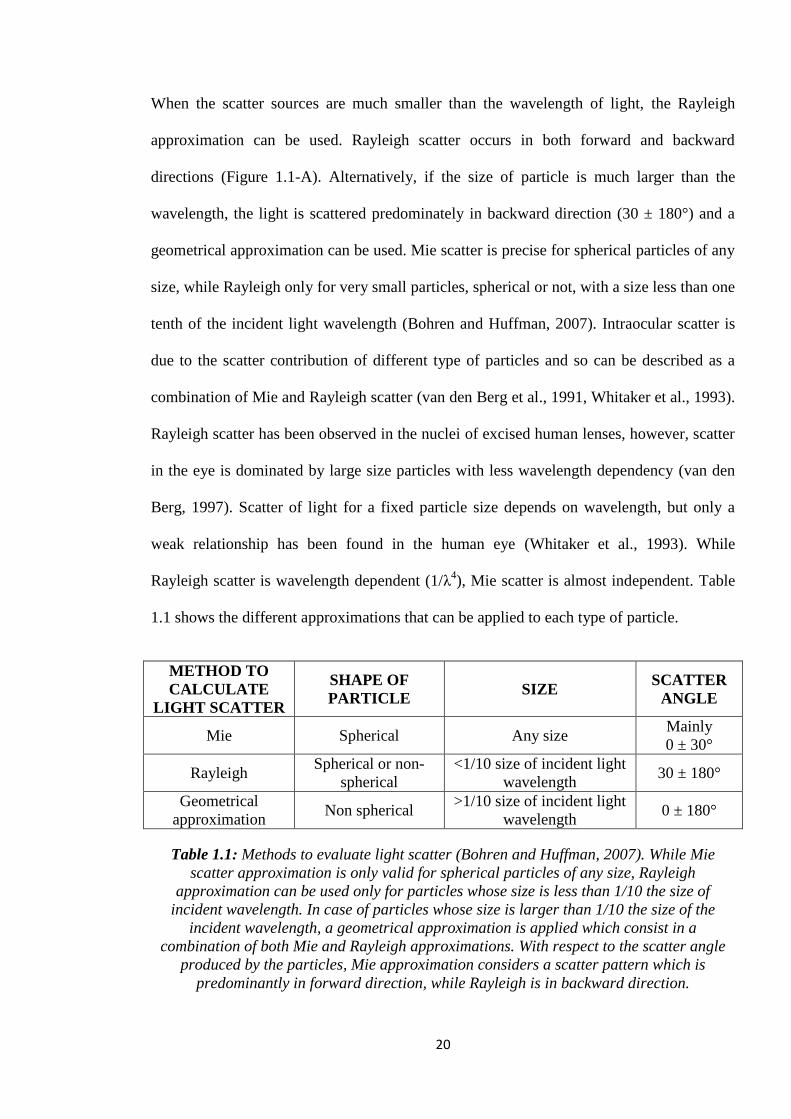
Table 1.1: Methods to evaluate light scatter (Bohren and Huffman, 2007). While Mie

scatter approximation is only valid for spherical particles of any size, Rayleigh

approximation can be used only for particles whose size is less than 1/10 the size of

incident wavelength. In case of particles whose size is larger than 1/10 the size of the

incident wavelength, a geometrical approximation is applied which consist in a

combination of both Mie and Rayleigh approximations. With respect to the scatter angle

produced by the particles, Mie approximation considers a scatter pattern which is

predominantly in forward direction, while Rayleigh is in backward direction. ................... 20

Table 1.2: Relationship between FLS (Log(s)) and the type of iris pigmentation measured

with C-Quant straylight meter for different angle eccentricities (Ө) (Van den Berg, 1995).

.............................................................................................................................................. 32

Table 1.3: Types of cataracts and mean C-Quant straylight value (Bal et al., 2011). ......... 36

Table 2.1: Summary of the mean values, standard deviation (SD), minimum and maximum

values obtained for C-Quant and the 3 different eccentricities of Straylight meter (S, M, L).

.............................................................................................................................................. 67

Table 2.2: Statistics for the differences of C-Quant (CQ) values minus straylight data for

each one of the three eccentricities of the Straylight meter (S-CQ, M-CQ, L-CQ) including

the Coefficients of agreement (COA). .................................................................................. 73

Table 2.3: Correlation coefficients (r) relating C-Quant values and the three eccentricities

measured with the Straylight meter (S, M and L). ............................................................... 73

Table 2.4: Calculation of VIF for the variables C-Quant (CQ) and the three eccentricities

of the Straylight meter S, M, and L. ..................................................................................... 74

Table 2.5: Multiple regression analysis using C-Quant as dependent variable and the three

eccentricities of the Straylight meter as independent variables. Coefficients, standard error

(Std. Error), t-value and correspondent p-value are also shown. ........................................ 74

Table 4.1: Types of density measurements and corneal thickness measurements available in

the basic version of Pentacam (software version 1.20r29). ............................................... 105

Table 4.2: Values (grey scale units) for the 3D corneal density for each one of the radial

eccentricities measured from the corneal apex and for each corneal area (mean±SD).

Anterior corneal zone comprises the first 120µm of corneal thickness and posterior

corneal covers the last 60 µm of corneal thickness. The centre of the cornea does not have

a fixed thickness and is calculated as the result of resting both anterior and posterior

corneal thickness from the total corneal thickness of the measured participant. Total values

are also shown for each of the eccentricities and corneal areas. ...................................... 108

11

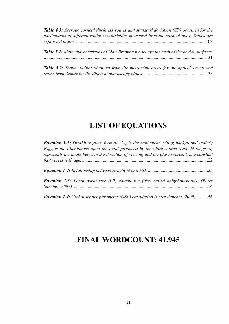
Table 4.3: Average corneal thickness values and standard deviation (SD) obtained for the

participants at different radial eccentricities measured from the corneal apex. Values are

expressed in µm. ................................................................................................................. 108

Table 5.1: Main characteristics of Liou-Brennan model eye for each of the ocular surfaces.

............................................................................................................................................ 131

Table 5.2: Scatter values obtained from the measuring areas for the optical set-up and

ratios from Zemax for the different microscopy plates. ..................................................... 135

LIST OF EQUATIONS

Equation 1-1: Disability glare formula. Leq is the equivalent veiling background (cd/m2)

Eglare is the illuminance upon the pupil produced by the glare source (lux). Ө (degrees)

represents the angle between the direction of viewing and the glare source. k is a constant

that varies with age. ............................................................................................................. 22

Equation 1-2: Relationship between straylight and PSF. .................................................... 25

Equation 1-3: Local parameter (LP) calculation (also called neighbourhoods) (Perez

Sanchez, 2009). .................................................................................................................... 56

Equation 1-4: Global scatter parameter (GSP) calculation (Perez Sanchez, 2009). ......... 56

FINAL WORDCOUNT: 41.945

12

ABBREVIATIONS LIST

BAT Brightness Acuity Tester

BLS Backward light scatter

BS Beam splitter

CIE Commission Internationale de I‟Eclairage

COA Coefficient of agreement

CS Contrast sensitivity

CSF Contrast sensitivity function

DP Double pass

ESD C-Quant standard deviation

FLS Forward light scatter

GRIN Gradient index media

GSP Global scattering parameter

HG Hartmanngram patterns

HS Hartmann-Shack Aberrometer

LASEK Laser assisted Subepithelial keratomileusis

LASIK Laser assisted in-situ keratomileusis

LOCS Lens Opacities Classification System

LP Local parameter

Max_SD Maximum standard deviation

MTF Modulated Transfer Function

OQAS Optical Quality Analysis System

OSI Objective scatter index

PMMA Polymethyl Methacrylate

PRK Photorefractive keratectomy

PSF Point Spread Function

Q Quality factor of the psychometric function – C-Quant

RPG Gas permeable rigid lenses

RK Radial keratotomy

SD/ESD Standard Deviation

VA Visual Acuity

VDB van den Berg Straylight meter

VIF Variance inflation factor

13

ABSTRACT

UNIVERSITY The University of Manchester

CANDIDATE´S FULL NAME Pablo Benito Lopez

DEGREE Doctor of Philosophy – Optometry

TITLE Measuring and modelling forward light scattering

in the human eye

DATE November 2015

BACKGROUND: Intraocular scatter is an important factor when considering the

performance of the human eye as it can negatively affect visual performances (e.g. glare).

However, and in contrast to other optical factors that also affect vision such as high order

aberrations, there is currently no efficient method to measure accurately and objectively the

amount and the angular distribution of forward light scatter in the eye. Various methods

and instruments exist to assess forward light scatter (FLS) but the relation between these

methods has rarely been quantified. In addition, FLS measurements obtained with existing

instruments cannot be related to any physiological factors due to the absence of a valid

model.

PURPOSE: To investigate the relations between some of the main methods to measure

forward light scatter, and to develop an experimental set-up for the objective measurement

of forward light scatter that could be ideally related to physiological parameters.

METHODS: After a short review of intraocular light scatter, the three main methods used

to assess forward light scattering are compared. In this sense, the C-quant (CQ) straylight

meter is compared to the van den Berg (VDB) straylight meter and the Hartmann-Shack

spot pattern analysis obtained from the Hartmann-Shack aberrometer. The potential of the

new Oculus Pentacam functionalities for providing information on backward light scatter

(BLS) are also investigated. Finally, an innovative prototype for objective assessment of

intraocular light scattering together with a scatter model of the eye is presented.

RESULTS and DISCUSSION: Although no significant relationship was found between

the different instruments considered (VDB straylight meter, CQ, Pentacam), our results

allowed us to clarify some possible confusion introduced by previously published results

and to illustrate the fact that existing commercial instruments such as aberrometers and the

Pentacam cannot be used to measure FLS without at least some major modifications

(hardware or software). Preliminary results with the prototype built in this study suggest

that it could be used for the objective measurement of intraocular light scatter. Relating this

measurement to physiological parameters stays however elusive, a fact that widens the

future scope of this research.

14

DECLARATION

No portion of the work referred to in this thesis has been submitted in support of an

application for another degree or qualification of The University of Manchester, or any

other university or institute of learning.

THESIS FORMAT

This thesis is presented in „Alternative Format‟. The decision to present the thesis

this way was taken as several of the chapters featured here had already been either

published, or prepared for submission to peer-reviewed journals. Where manuscripts based

on these chapters have been published, or submitted for publication in a refereed journal it

is indicated on the first page of the chapter. The author‟s contribution to the work presented

in each chapter is also identified on the first page of each chapter.

15

COPYRIGHT STATEMENT

i. The author of this thesis (including any appendices and/or schedules to this thesis)

owns certain copyright or related rights in it (the “Copyright”) and s/he has given

The University of Manchester certain rights to use such Copyright, including for

administrative purposes.

ii. Copies of this thesis, either in full or in extracts and whether in hard or electronic

copy, may be made only in accordance with the Copyright, Designs and Patents Act

1988 (as amended) and regulations issued under it or, where appropriate, in

accordance with licensing agreements which the University has from time to time.

This page must form part of any such copies made.

iii. The ownership of certain Copyright, patents, designs, trade marks and other

intellectual property (the “Intellectual Property”) and any reproductions of

copyright works in the thesis, for example graphs and tables (“Reproductions”),

which may be described in this thesis, may not be owned by the author and may be

owned by third parties. Such Intellectual Property and Reproductions cannot and

must not be made available for use without the prior written permission of the

owner(s) of the relevant Intellectual Property and/or Reproductions.

iv. Further information on the conditions under which disclosure, publication and

commercialisation of this thesis, the Copyright and any Intellectual Property and/or

Reproductions described in it may take place is available in the University IP

Policy (see http://documents.manchester.ac.uk/DocuInfo.aspx?DocID=487 ), in any

relevant Thesis restriction declarations deposited in the University Library, The

University Library‟s regulations (see

http://www.manchester.ac.uk/library/aboutus/regulations) and in The University‟s

policy on Presentation of Theses.

http://documents.manchester.ac.uk/DocuInfo.aspx?DocID=487

http://www.manchester.ac.uk/library/aboutus/regulations

16

ACKNOWLEDGEMENTS

Firstly, I would like to thank my supervisors Dr Hema Radhakrishnan and Dr

Vincent Nourrit for their support, guidance and encouragement. Their help has been really

important for me and for the development of the thesis.

I am grateful to my relatives. They have made an invaluable contribution, either

with moral support or any other kind.

Finally, I want to thank the big group of people and friends I have met in

Manchester, those I have shared great moments with and those that helped me in many

moments.

17

1. INTRODUCTION

1.1 OVERVIEW

The main optical factors degrading the quality of the retinal image, and hence our

vision, are diffraction, aberrations and scatter. Diffraction is an optical phenomenon related

to the finite size of the pupil and thus inherent to any optical system. For the human eye,

diffraction is a limiting factor when the pupil diameter is approximately less than 2.4 mm

(Charman, 1991, Rovamo et al., 1998). Aberrations, usually divided into monochromatic

and polychromatic aberrations (Donnelly and Applegate, 2005), can be measured

efficiently using different wave front sensing technique (e.g. Hartmann-Shack (Miranda et

al., 2009), pyramid (Mierdel et al., 2001), curvature sensor (Diaz-Douton et al., 2006)).

Among them, low order aberrations can be easily corrected by various means including

spectacles, contact lenses, intraocular lenses or refractive surgery. Light scatter is due to

small scale inhomogeneities within the ocular media, whose refractive indices with respect

to the surrounding media modify the original trajectory of the light inside the eye. These

inhomogeneities will affect light propagation within the eye and degrade the retinal image

quality. An example of such inhomogeneities is the activation of keratocytes in laser

surgery. When quiescent, their refractive index is similar to the surrounding stroma.

However when activated, their composition changes and therefore their refractive index.

As a result of this change, light is deviated and does not participate “correctly” (according

to the optical ray tracing) to the retinal image‟s formation process.

Intraocular scatter levels play an important role next to visual acuity in defining our

overall visual performance (Donnelly and Applegate, 2005) and many studies that were

published during the last decades presented possible clinical applications, from controlling

18

the cataract progression to diagnosing different types of ocular pathology (see the

following review papers as reference (Pinero et al., 2010, van den Berg et al., 2013)).

However, the objective and accurate assessment of intraocular light scatter remains a

difficult task when it is compared to the measurement of aberrations and diffraction. In

addition, measurements obtained with existing instruments cannot be related to any

physiological factors. Obtaining accurate and reliable measurements, and being able to

relate them to the source of scatter through a model, would allow for a better understanding

and assessing of how various factors (e.g. old age, ocular pathologies) may lead to a

decrease of visual performances (e.g. disability glare) through increased scatter. The

development of a prototype for objective measurement of forward light scatter (FLS) and

the creation of a numerical eye model to relate the experimental data to physiological

parameters is therefore the main objective of this PhD research.

This first chapter intends to give a review of the work that has been done in the

field, clarify important concepts, summarize the scatter structures within the human eye

and main techniques used on the assessment of that intraocular scatter that were necessary

for the research conducted during this PhD project.

1.2 WHAT IS INTRAOCULAR LIGHT SCATTER?

As stated above, ocular scatter can be defined as the change in the trajectory that

light experiences inside the eye due to the presence of inhomogeneities within the ocular

media. Another definition of intraocular light scatter is “the percentage of reflected,

diffracted or refracted light along the optical media of the eye due to the differences in

19

refractive index of particles in the trajectory of the incident beam” (Donnelly and

Applegate, 2005).

Intraocular scatter is usually divided in two different categories, depending on the

change in trajectory of the incident light. When the angle of deviation is less than 90°, it is

called forward light scatter (FLS). FLS reaches the retina and produces a veiling luminance

(also called straylight), reducing in this way the contrast of the retinal image and possibly

the visual performance (Donnelly and Applegate, 2005). On the contrary, when the

deviation angle is more than 90°, light does not reach the retina. In this case, the

phenomenon is called backward light scatter (BLS).

Figure 1.1: Types of scatter produced by different sizes of particles: Scatter produced by

small particles whose size is less than 1/10 the size of the incident wavelength) is

principally Rayleigh (A) and produces a homogenous scatter pattern around the particle.

For larger particles than the incident wavelength Mie scatter takes place (B and C). The

Mie scatter pattern produced by large particles is narrower in forward direction when the

particle is larger (C).

Physically, intraocular scatter can be complex since it depends on the shape, size

and refractive index of the scatter structures with respect of their surrounding media. The

shape of these elements is usually considered to be spherical in order to use Mie scatter

modelling solutions (Mie, 1908) and the associated approximations. When the size of the

particle is close to the wavelength, Mie scatter approximation takes place and the

distribution of scattered light is predominantly forward (Figure 1.1-B and Figure 1.1-C).

20

When the scatter sources are much smaller than the wavelength of light, the Rayleigh

approximation can be used. Rayleigh scatter occurs in both forward and backward

directions (Figure 1.1-A). Alternatively, if the size of particle is much larger than the

wavelength, the light is scattered predominately in backward direction (30 ± 180°) and a

geometrical approximation can be used. Mie scatter is precise for spherical particles of any

size, while Rayleigh only for very small particles, spherical or not, with a size less than one

tenth of the incident light wavelength (Bohren and Huffman, 2007). Intraocular scatter is

due to the scatter contribution of different type of particles and so can be described as a

combination of Mie and Rayleigh scatter (van den Berg et al., 1991, Whitaker et al., 1993).

Rayleigh scatter has been observed in the nuclei of excised human lenses, however, scatter

in the eye is dominated by large size particles with less wavelength dependency (van den

Berg, 1997). Scatter of light for a fixed particle size depends on wavelength, but only a

weak relationship has been found in the human eye (Whitaker et al., 1993). While

Rayleigh scatter is wavelength dependent (1/λ4), Mie scatter is almost independent. Table

1.1 shows the different approximations that can be applied to each type of particle.

METHOD TO

CALCULATE

LIGHT SCATTER

SHAPE OF

PARTICLE SIZE

SCATTER

ANGLE

Mie Spherical Any size Mainly

0 ± 30°

Rayleigh Spherical or non-

spherical

<1/10 size of incident light

wavelength 30 ± 180°

Geometrical

approximation Non spherical

>1/10 size of incident light

wavelength 0 ± 180°

Table 1.1: Methods to evaluate light scatter (Bohren and Huffman, 2007). While Mie

scatter approximation is only valid for spherical particles of any size, Rayleigh

approximation can be used only for particles whose size is less than 1/10 the size of

incident wavelength. In case of particles whose size is larger than 1/10 the size of the

incident wavelength, a geometrical approximation is applied which consist in a

combination of both Mie and Rayleigh approximations. With respect to the scatter angle

produced by the particles, Mie approximation considers a scatter pattern which is

predominantly in forward direction, while Rayleigh is in backward direction.

21

When a ray of light passes through a particle inside the eye, that ray can pass the particle

without modifying its trajectory or be scattered. The overall light scattered is proportional to

the intensity of the incoming light and its angular distribution will depend on the scatter

source (size, shape, refractive index and spatial distribution). Light has also an associated

energy. This energy can be partially or totally absorbed by a particle the light is passing

through. Different ocular structures have been found to absorb determined wavelengths

(Miller et al., 2005).

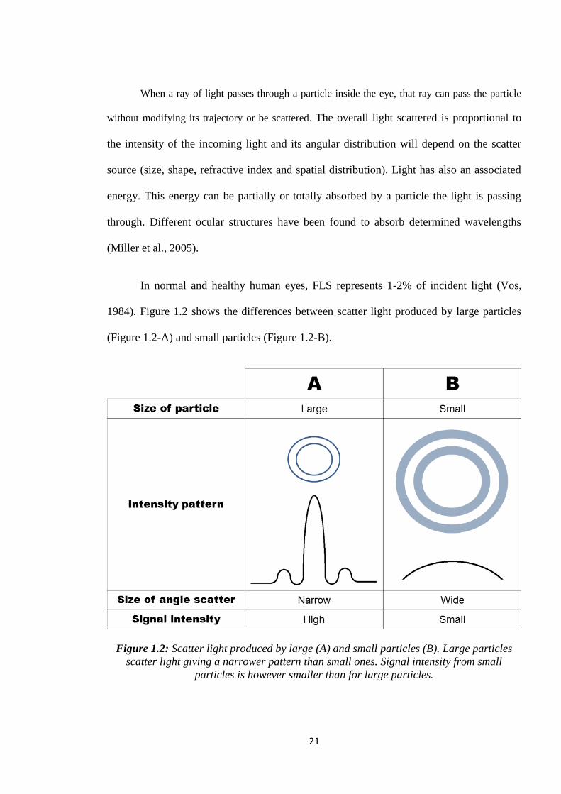
In normal and healthy human eyes, FLS represents 1-2% of incident light (Vos,

1984). Figure 1.2 shows the differences between scatter light produced by large particles

(Figure 1.2-A) and small particles (Figure 1.2-B).

Figure 1.2: Scatter light produced by large (A) and small particles (B). Large particles

scatter light giving a narrower pattern than small ones. Signal intensity from small

particles is however smaller than for large particles.

22

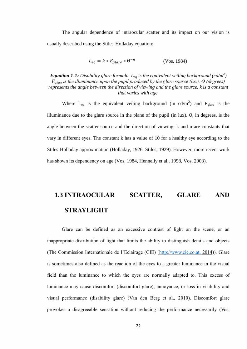
The angular dependence of intraocular scatter and its impact on our vision is

usually described using the Stiles-Holladay equation:

(Vos, 1984)

Equation 1-1: Disability glare formula. Leq is the equivalent veiling background (cd/m2)

Eglare is the illuminance upon the pupil produced by the glare source (lux). Ө (degrees)

represents the angle between the direction of viewing and the glare source. k is a constant

that varies with age.

Where Leq is the equivalent veiling background (in cd/m2) and Eglare is the

illuminance due to the glare source in the plane of the pupil (in lux). , in degrees, is the

angle between the scatter source and the direction of viewing; k and n are constants that

vary in different eyes. The constant k has a value of 10 for a healthy eye according to the

Stiles-Holladay approximation (Holladay, 1926, Stiles, 1929). However, more recent work

has shown its dependency on age (Vos, 1984, Hennelly et al., 1998, Vos, 2003).

1.3 INTRAOCULAR SCATTER, GLARE AND

STRAYLIGHT

Glare can be defined as an excessive contrast of light on the scene, or an

inappropriate distribution of light that limits the ability to distinguish details and objects

(The Commission Internationale de I‟Eclairage (CIE) (http://www.cie.co.at, 2014)). Glare

is sometimes also defined as the reaction of the eyes to a greater luminance in the visual

field than the luminance to which the eyes are normally adapted to. This excess of

luminance may cause discomfort (discomfort glare), annoyance, or loss in visibility and

visual performance (disability glare) (Van den Berg et al., 2010). Discomfort glare

provokes a disagreeable sensation without reducing the performance necessarily (Vos,

http://www.cie.co.at/

23

2003). Disability glare occurs when the incoming light from the bright source is scattered

by the ocular lens, forming a veiling luminance over the retina, reducing the contrast of the

final retinal image or even producing almost total blindness when high intensity glare

sources are positioned near the eyes (Vos, 1984, van den Berg, 1995). The effect of

disability glare is mainly due to intraocular scatter of light (van den Berg et al., 2009b).

Thus, the evaluation of disability glare through the assessment of straylight became a CIE

standard (Vos, 1984).

1.4 INTRAOCULAR SCATTER AND CONTRAST

SENSITIVITY

Contrast sensitivity (CS) is another important factor used to evaluate vision

performances. CS determines the lowest level of contrast that can be detected for a patient

for a fixed stimulus size. CS is thus different from visual acuity (VA). CS depends on the

size and the contrast of the target while VA depends only on the size since the contrast of

the target is always fixed (black and white or 98% to 100%). For this reason, a score of

20/20 in Snellen test, which means a normal VA, does not necessarily mean a good quality

of vision or visual performance.

CS can be estimated through different methods. A good correlation was found

between low contrast sensitivity scores across a range of spatial frequencies and intraocular

light scatter (Barbur et al., 1999, Aguirre et al., 2007). This result is not surprising since the

main effect of FLS is the reduction of contrast of the retinal image. In this context, glare

tests which assess the reduction of contrast of the retinal image could be seen as an indirect

way to assess FLS. In this sense, the agreement between a measure of glare and FLS

24

(results from the van den Berg straylight meter being taken as gold standard) has been

investigated for various glare test. The best agreement was obtained when using the Pelli-

Robson chart together with the Brightness Acuity Tester (BAT) (glare test) in the presence

of a glare source (Elliott and Bullimore, 1993).

1.5 SCATTER AND POINT SPREAD FUNCTION

Point spread function (PSF) is the distribution of light obtained in the retina from

an ideal point source of light. The PSF describes the quality of the visual system, and as

stated above, is degraded by aberrations, diffraction and light scatter. Two different

scenarios illustrating a perfect (Figure 1.3-a) and a degraded (Figure 1.3-b) PSF are

depicted in Figure 1.3.

Figure 1.3: Retinal PSF from a point light source. A shows the image from that point in

ideal conditions while B shows the image from that point considering aberrations,

diffraction and scatter.

The PSF can be related mathematically to intraocular light scatter (van den Berg et

al., 2009a). In these calculations, the area within 1±90° around the centre of the PSF is

affected by intraocular scatter and receives around 10% of the light reaching the retina

(Vos, 1984, Franssen et al., 2007). Equation 1-2 relates straylight and PSF between 1-90°

(van den Berg, 1995).

25

( ) ( ) F( ) (van den Berg, 1995)

Equation 1-2: Relationship between straylight and PSF.

Where “s” is the straylight parameter (in degrees2/sr) and Ө is the angle subtended

between the glare source and the direction of viewing in degrees. The size of the pupil only

affects the parameter “s” if the ocular media is not homogeneous (van den Berg, 1995).

Figure 1.4 shows a graph corresponding to the relationship obtained between PSF and

scatter angle for a subject (Ginis et al., 2012).

Figure 1.4: Relationship between PSF (Log (PSF)) and the scatter angle Ө (in degrees)

obtained for a subject using a double pass system (Ginis et al., 2012). As it can be seen on

the figure, Log(PSF) becomes smaller as the measured scatter angle increases.

26

1.6 SOURCES OF SCATTER

As previously stated, the amount of light forwardly scattered by the human eye

(Figure 1.5) correspond to approximately 1-2% of incoming light (Vos, 1984). For a

healthy eye, the contribution of FLS by the cornea is up to 30% (Vos and Boogaard, 1963)

and 5% more for iris and scleras from lightly pigmented eyes (van den Berg, 1995). The

contribution of the crystalline lens is around 40% though this value can be much higher in

case of advancing age or cataract (Bettelheim and Ali, 1985). The retina contributes up to

20% (Delori, 2004). Floating particles in the vitreous increases the amount of light scatter

in case of symptomatic eyes (Castilla-Marti et al., 2015). Since the intraocular scatter is

mainly due to the cornea, the iris, the lens and the retina, we review their respective scatter

structures in the following subsections as it will be useful to develop a numerical model of

intraocular scatter.

Figure 1.5: Light scatter structures of the human eye. Major light scatter structures are

the cornea (30% of the incident light), crystalline lens (40%) and the retina (20%). Light

scatter through the iris in light pigmented eyes and through the sclera can be up to 5% of

the incident light.

27

1.6.1 CORNEA

The cornea can be divided in 6 different layers (Figure 1.6). The layer situated next

to the tear film is the epithelium, with a thickness of approximately 40µm. The more

internal cells of this layer are attached to the basement membrane (0.05µm thickness),

which is over the Bowman‟s layer (10µm). Bowman‟s layer is formed by a collagen matrix

with no cells. The stroma (500µm thick) occupies 90% of the corneal thickness and is

situated between the Bowman‟s layer and the Descemet‟s membrane. Behind the

Descemet‟s membrane is the endothelium, a single layer of cells. Both, the Descemet‟s

membrane and the endothelium have a thickness of 10µm (Freund et al., 1986). The

stromal cornea is composed of about 250 lamellae with 2µm thickness each (Hogan et al.,

1971). Lamellae are made of parallel collagen fibrils with a thickness of 0.025 µm each

and a refractive index of 1.47. Lamellae have regular shape and size and they are floating

in a matrix of refractive index 1.354 (Maurice, 1969). Fibrils extend across the cornea and

those from lamellae make large angles with others from adjacent lamellae (Freund et al.,

1986). The transparency of the cornea is assumed to be due to the regularity of separation

of fibrils within the stroma of the cornea (Maurice, 1957). However, the array of fibrils is

not infinite, and because the separation width is not insignificant compared to the

wavelength, some scatter is wavelength dependent (Hart and Farrell, 1969).

28

Figure 1.6: Structure of the cornea depicted from the epithelial to the endothelial layer

(epithelial layer, Bowman´s layer, stoma, Descemet´s membrane and endothelial layer).

Stroma is composed of regularly separated fibrils. Anatomically, both fibrils and

keratocytes are parallel to the different layers of the cornea, but have been depicted

perpendicularly for illustration purposes.

The integrity of the endothelial layer has also been found to be crucial in the

maintenance of the stromal transparency, acting as a shield (Steele, 1999). Between fibrils,

there are flat cells of 15µm each called Keratocytes, occupying 3-5% of corneal volume

and 9-17% of corneal stromal volume (Hahnel et al., 2000). There are around 2.0-3.5

million keratocytes in the corneal stroma (Moller-Pedersen, 1997) with a thickness of 1 µm

of nuclei and several cell-processes of up to 50µm long, giving the keratocyte a stellated

shape that covers an area of about 1000 µm2 in the frontal plane (Hahnel et al., 2000).

However, some authors have found a keratocyte size covering an area of 78-211 µm2

(Prydal et al., 1998). The density of keratocytes is about 20522 ± 2981 cells/mm3 (mean ±

standard deviation) (Patel et al., 2001). Light travelling through the cornea might have to

pass about 100 layers of keratocytes with their scatter properties (density, volume and size

estimates), and therefore, the development of an optical model eye including the scatter

properties of the keratocytes seems to be reasonable (Moller-Pedersen, 2004).

29

Another study found that for scatter angles larger than 30° with respect to the visual

axis, the main corneal layer contributing to scatter is the stroma (70%), and the remaining

30% might be probably related to scatter by the epithelial layer, the endothelial layer,

Bowman‟s layer and stromal keratocytes (Freund et al., 1986). Other studies have shown

that major sources of light scatter within the cornea are the endothelium and the epithelial

cell layer, with scatter from the stroma limited to the keratocytes nuclei and not to the

broad cell bodies (Jester, 2008). A study analysing corneas from postnatal rabbits found a

good relationship between decreased density of keratocytes and reduction of light scatter

(Jester et al., 2007).

Several studies investigated the wavelength dependency of corneal transparency.

As previously stated, it is related to the space between structures of different refractive

index (McCally and Farrell, 1988) and the magnitude of fluctuation of refractive index of

structures. In fact, if the space separating scatter structures such as fibrils is small or less

than half of visible light wavelength (400-700nm), hence the environment is transparent

(Benedek, 1971).

1.6.2 CRYSTALLINE LENS

Previous studies have found that scatter in the crystalline lens is due to the change

of refractive index between the surrounding cytoplasm and cell membranes, the increase in

the separation of fibres (Kerker, 1969), or the aggregation of protein molecules (Bettelheim

and Ali, 1985, Hemenger, 1992, Whitaker et al., 1993).

The crystalline lens is composed of a biconvex lens capable of modifying its shape

to perform its main objective, the accommodation mechanism. The crystalline lens can be

30

defined as a matrix of fibres (Figure 1.7) placed very closely to each other (Trokel, 1962).

Recent investigations of crystalline lens fibres and their refractive index have shown that

fibres produce significant scatter and are homogenously spaced in the lens cortex (i.e. the

peripheral part of the lens). This order of the fibers makes the crystalline lens more

transparent. However, the fibers can act as a diffraction grating that is responsible in some

circumstances to the lenticular halo (Charman, 1991b).

Figure 1.7: Structure of the crystalline lens. The crystalline lens is internally composed of

a matrix of fibers which are equally distributed and surrounded by the cytoplasm. Cells

from the cytoplasm can migrate to different areas of the crystalline lens and create large

molecules that produce light scatter.

The refractive index of the crystalline lens is not constant and presents a gradient

index profile (GRIN) that improves the focusing properties of the lens. The refractive

index of the fibres‟ membrane and cytoplasm decreases from the centre (1.409) towards

the periphery (n = 1.380 (Kasthurirangan et al., 2008)). This difference in refractive indices

is attributed to proteins from the fibres cytoplasm (Lovicu and Robinson, 2004). The

transparency of the crystalline lens is attributed to the high concentration of proteins and

their short-range-order interactions between them, that produce destructive interferences

eliminating “virtually” the light scatter (Delaye and Tardieu, 1983).

31

It was also noted that the concentration of large particles need to be high to explain

the amount of light scattered forwardly by the lens (Bettelheim and Ali, 1985). Continuing

with this investigation, many studies have tried to identify the effect on scatter produced by

proteins packed in the cytoplasm of the crystalline fibre cells (Gilliland et al., 2004). In this

sense, the Rayleigh-Gans approximation allows describing light scatter when a scatter

source has a refractive index similar to the one of the surrounding media. Given this

situation, if the size of the scatter source increases, FLS becomes greater and BLS

decreases (Kerker, 1969). This confirms that the aggregation of proteins molecules in the

crystalline lens produces an increase of FLS. In the same way, scatter of light through

cataracts is probably due to: the differences in the refractive index of the lens fibres

(Hemenger, 1992); the aggregation of protein molecules in the crystalline‟s nucleus

(Bettelheim and Ali, 1985) and the posterior migration of cells from the epithelia, creating

large organelles and eventually, posterior subcapsular cataracts (George, 2005).

These proteins, once they are produced, stay in the fibers and may suffer from some

modifications such as cross-linking, creating proteins aggregates and changing their

refractive indices, leading to an opacification and an increase in FLS (Hanson et al., 2000).

With ageing, these proteins can suffer from oxidation as well, damaging the fiber cell

membranes, and resulting in larger particles than the aggregates produced by protein cross-

linking (Gilliland et al., 2004). These large particles which are called Multillamellar bodies

(MLBs) (Gilliland et al., 2001), have a spherical shape and occupy a volume lower than

0.005% of the membrane. With an average diameter 2.4µm, they are located in the

equatorial axis of the nucleus of the lens. MLBs are 7.5 times more frequent in cataracts

than transparent crystalline lens (Gilliland et al., 2001), and they show Mie scatter (van den

Berg, 1997, van den Berg and Spekreijse, 1999).

32

Other studies have found that MLBs have an average diameter of 2.7µm and are

coated by 3-10 thin bilayers with a thickness of 5µm each. The nucleus of the MLBs has

an index of refraction of 1.49, while the coating might be 1.40 (Costello et al., 2007).

1.6.3 IRIS, SCLERA AND UVEAL TRACT

A small fraction of the total FLS (1% or less depending on the colour of the eye

(van den Berg et al., 1991)) can be attributed to illumination through the ocular wall.

Greater scatter levels have been found in lightly pigmented eyes than in dark brown irises

of non-Caucasians (Van den Berg et al., 1990, Elliott et al., 1991, van den Berg et al.,

1991, de Waard et al., 1992). In fact, blue eyes from Caucasians produce about 18% more

light scatter than brown Caucasian eyes (van den Berg et al., 1991).

In the next table (Table 1.2), some results from a study are presented in which a

strong relationship between FLS and the type of iris pigmentation was found (van den

Berg, 1995).

No. Mean

Age

Log(s)

Ɵ=3.5° Ɵ=7° Ɵ=13.6° Ɵ=25.4°

Caucasians blue eyed 33 33.5 0.88 0.80 0.91 1.20

Caucasians blue-green

eyed 6 39.5 0.87 0.81 0.91 1.16

Caucasians brown eyed 19 37.7 0.82 0.74 0.81 1.07

Pigmented non-

Caucasians 20 34.2 0.74 0.65 0.70 0.81

All Caucasians 109 20-82

Table 1.2: Relationship between FLS (Log(s)) and the type of iris pigmentation measured

with C-Quant straylight meter for different angle eccentricities (Ө) (Van den Berg, 1995).

33

With reference to the uveal tract, transmittance of light through this media was

found reduced by 0.2-1% due to the different absorption properties of the melanine in

visible spectrum (van den Berg et al., 1991).

1.6.4 RETINA

The retina is made of several layers that partially reflect the light received. Hence,

some of the incident light will be scattered backward or laterally. This scatter depends on

the level of pigmentation of the pigmented retinal epithelium and of the choroid (Vos and

Boogaard, 1963, Vos, 1984, Franssen et al., 2007) and is thus wavelength dependent

(mainly due to the presence of melanin and oxyhaemoglobin (Hodgkinson et al., 1994).

Other studies found that retinal straylight increases with ageing and also with the axial

length of the eye (Rozema et al., 2010).

The retina produces a Rayleigh type scatter on light, which is wavelength

dependent (Stiles, 1929) and proportional to λ-4

(McCally and Farrell, 1988).

1.7 FACTORS AFFECTING INTRAOCULAR LIGHT

SCATTER

In the previous section, the physical structure of the main sources of intraocular

scatter was described, i.e. the cornea, transillumination through the iris, the crystalline lens

and the retina. However, intraocular scatter can also be affected by several additional

factors such as physiological changes related to age, pathologies or refractive corrections.

The purpose of this section is to review these different factors.

34

1.7.1 PHYSIOLOGICAL

Numerous studies investigating the relation between scatter and age have reported

an increase of intraocular scatter with age (Van Den Berg et al., 2007, Rozema et al.,

2010). This increase is assumed to be due to changes in the crystalline fibers and the

aggregation of protein molecules, especially in the cortex and nucleus (Allen and Vos,

1967).

FLS in a 70 years old person with normal ocular media has been found to be about

2.0 to 2.57 times higher than in a 20 years old person (Whitaker et al., 1993). Major

increments of FLS start after 40 years old (Wolf, 1960, Elliott et al., 1991, Hennelly et al.,

1998), coinciding with a study in which it was found that the transmittance through the

ocular media did not change significantly between the first and third decade (Coren and

Girgus, 1972, Norren and Vos, 1974).

Aging also produces the yellowing of the crystalline lens with its consequent

reduction in transmission (Said and Weale, 1959), a loss of pigment from the iris and a

reduction of corneal transparency (Olsen, 1982, Smith et al., 1990).

1.7.2 PATHOLOGICAL

The increase of intraocular light scatter has been associated with various medical

conditions. Some of these conditions, including the most common ones, are listed

hereafter.

• Ocular pigment disorders: As stated before, the level of pigmentation of the

ocular wall and iris have an influence on the level of intraocular light scatter. In this sense,

35

the transillumination through the iris wall was found to decrease from around 1% in a

light-blue eye to two orders of magnitude lower in a dark brown eye (van den Berg et al.,

1993). In this context, it is not surprising that some conditions such as albinism or pigment

dispersion syndrome might produce an increase in the transmittance through the ocular

wall and iris, leading to an increase of FLS (Van den Berg et al., 1990).

• Dystrophies, opacities and corneal oedema: An increase of both FLS and BLS has

been found on corneal scars that produce lower density opacities. These low density

opacities were found to produce greater levels of FLS than high density ones (van den

Berg, 1986). As a consequence, Woodward, in 1996 said that tattooing the scars may

improve the visual performance (Woodward, 1996). In addition, there are some corneal

dystrophies such as granular dystrophy that produce changes in the transparency of the

cornea and therefore, an increase of the intraocular scatter (van den Berg, 1986).

Keratoconus is a type of corneal dystrophy that is related with the increase of ocular light

scatter and produces a change of the collagen fibrils in the corneal stroma, making it

thinner (Meek et al., 2005). The increase of scatter could be related to the structural

degradation of the cornea, in which, alterations of epithelia and stromal changes of

keratocytes and lamellae may occur (Jinabhai et al., 2012).

• Cataracts. Cataracts are the result of the opacification of the crystalline lens. Age

related cataracts are the most common, but a combination of nuclear or posterior

subcapsular cataracts may be seen. The increase of the intraocular light scatter due to

cataracts is a consequence of the nuclear sclerosis, which may be defined as “the alteration

of the crystalline lens metabolism to allow changes in the concentrations of insoluble

protein” (George, 2005). In the crystalline nucleus, oxidation of soluble and insoluble lens

proteins might be a result of long-wavelength radiation. The sclerosis of the nucleus

36

produces a cross-linking of proteins that increases the optical density and decreases the

nucleus transparency (Gilliland et al., 2004).

The amount of light scatter produced by different types of cataracts has been

related to the LOCS III cataract classification (Chylack et al., 1993, Donnelly et al., 2004).

In Table 1.3, straylight values for different types of cataracts are represented.

Cataract type Straylight (log(s))

Nuclear 1.56

Cortical 1.52

Nuclear-cortical 1.72

Posterior subcapsular 1.83

Table 1.3: Types of cataracts and mean C-Quant straylight value (Bal et al., 2011).

Sometimes, there is an increase of FLS after the extraction of the cataract and the

implantation of the intraocular lens. This increase is usually related to the apparition of

opacities on the posterior surface of the capsular bag (also called posterior capsule

opacification) due to the proliferation of epithelial cells. This problem can be easily

addressed with a Neodymium-Yag laser capsulotomy, which is used to clean the posterior

capsule of the crystalline lens and clear the optical axis.

Regarding the type of cataract, the effects of a posterior cataract on vision are much

worse than those from a cataract of same size situated anteriorly. This phenomenon has

often been explained by the nearness of nodal points of the eye and the scatter centre.

However, the reasons why this has different consequences on the vision of the patient are

not well understood (George, 2005).

• Aphakia and pseudophakia. An aphakic, or pseudophakic eye, is an eye from

which the crystalline lens has been removed surgically. After that process, an intraocular

37

lens is then usually inserted in replacement. This implant can be itself a source of scatter.

The scatter is then related to the physical and optical properties of the lens (e.g.

multifocality, diffraction by edges, etc.) (Martin, 1999). As a consequence of the

intraocular scatter produced by the intraocular lens, some aphakes and pseudoaphakes

patients have a very low contrast sensitivity at mid and high spatial frequencies compared

to age-matched patients with normal eyes (Hess et al., 1985, Weatherill and Yap, 1986).

• Ocular surgery: Nowadays, many types of corneal surgery have been developed to

correct for the refractive error by modifying the corneal shape. Such surgeries often lead to

a temporary or permanent increase in FLS associated with the healing process. A large

number of studies focused on this topic, particularly in relation with Lasik (Laser assisted

in-situ keratomileusis). Main studies and findings are reviewed below and refer the reader

to the following document for further details (Chisholm, 2003).

Radial Keratotomy (RK) is a technique for the treatment of myopia (Fyodorov and

Durnev, 1979) and consists of the creation of radial incisions with a diamond micrometer

through 95% of the thickness of the cornea in the mid-peripheral and peripheral cornea,

keeping an area of three to four millimetres in the centre (Waring et al., 1985). Intraocular

scatter is significant during the next six months after the surgery, decreasing gradually over

time (Veraart et al., 1995). After that period, scatter becomes significant only for larger

pupil sizes that let surgery incisions to be present in pupil diameter.

In photorefractive keratectomy (PRK), an ablation is produced in the anterior

lamina of cornea and just after, a small lamina layer of epithelium is removed. After a few

days, keratocytes from the epithelium create a new layer. This migration of keratocytes

produces an increase in FLS (Lohmann et al., 1991). The major problem attributed to PRK

is the apparition of an opacification known as “haze”, which normally starts after two to

38

four weeks after surgery and disappears in twelve months in most cases (McDonald et al.,

1989, Seiler et al., 1990, Lohmann et al., 1991). At first, the structure of haze is

homogeneous but, becomes heterogeneous with time. These heterogeneous areas are

subject to present more light scatter than the homogeneous ones (Maldonado et al., 1996).

Patients with higher myopia degrees normally show a more intense and persistent haze

(Gartry et al., 1992, O'Brart et al., 1994, Maldonado et al., 1996).

Laser assisted in-situ keratomileusis (LASIK) is a technique in which a small flap

of the corneal tissue is cut using a microkeratome. A stromal layer is then ablated using an

excimer laser and the epithelial flap repositioned. This technique does not allow collagen

or extracellular matrix formation due to the preservation on Bowman´s membrane. This is

the reason why LASIK adds less light scatter to the cornea compared to other refraction

techniques, such as PRK. However, patients with anterior corneal cell density reduced

because of LASIK presented greater levels of intraocular straylight than patients without

undergoing any type of refractive surgery (Nieto-Bona et al., 2010).

Laser Assisted Subepithelial Keratomileusis (LASEK) involves preserving the

extremely thin corneal epithelial layer by lifting it from the eye's surface before laser

energy is applied for reshaping. After the LASEK procedure, the epithelium is replaced on

the eye's surface. Straylight increases to some degree after hyperopic LASIK and LASEK,

but this increase was not found to be statistically significant (Lapid-Gortzak et al., 2010).

• Stress: Some protein associated with stress might migrate and generate an

aggregation of proteins to the crystalline lens. This continuous aggregation of proteins

because of the stress increases the scatter of the lens and eventually might result in the

formation of a cataract (Shinohara et al., 2006).

39

• Others: Anterior uveitis or uncorrected myopia greater than -6.00D has been

associated with an increase of FLS (van der Heijde et al., 1985, van den Berg, 1986).

1.7.3 OPTICAL

In the previous sections, we reviewed the physiological factors related to

intraocular scatter, whether natural or pathological. Since 75% of the population in the

Western world uses some sort of vision corrections (Vision Council of America,

http://www.thevisioncouncil.org/, 2014), the scatter properties of such corrections are

reviewed hereafter.

Ocular lubricants: There was not found any relationship between intraocular scatter

and the use of ocular lubricants (Veraart et al., 1992). However, a recent study found that

lubricant eye-drops reduce ocular scatter in patients with mild to moderate dry eye (Diaz-

Valle et al., 2012).

Spectacles and contact lenses: The straylight produced by clean spectacle lenses is

not significant compared to the total amount of FLS (De Wit and Coppens, 2003).

However, there is strong evidence that contact lenses may increase light scatter (Bergevin

and Millodot, 1967, Applegate and Wolf, 1987, Elliott et al., 1991, Lohmann et al., 1993).

In addition, wearing contact lenses may cause a corneal oedema if the transmissibility of

the material of the lens is poor, they are worn for too long, or the lenses have a low

permeability (Woodward, 1996). Elliott found in 1991 (Elliott et al., 1991) more

intraocular scatter in rigid contact lens wearers than in soft lens wearers, but when the

lenses were removed, the trend was reversed. These studies suggest that the increase of

intraocular light scatter in a rigid lens is due to the material or the design. The increase in

http://www.thevisioncouncil.org/

40

soft lenses is a result of physiological changes such as corneal oedema and the variation of

levels of intraocular scatter is not significant (Elliott et al., 1991).

Wavelength dependency: Intraocular scatter has been proven to be dependent on

wavelength (Wooten and Geri, 1987, Whitaker et al., 1993). In one study, the retinal

straylight was measured from 625 to 457nm. It was found that well pigmented eyes such as

young negroids had nearly clear λ-4

wavelength dependence. However, in less pigmented

eyes (blue eyed Caucasians), the λ-4

wavelength dependence was not present (Coppens et

al., 2006).

1.8 METHODS TO MEASURE INTRAOCULAR LIGHT

SCATTER

Numerous methods can be found in the literature to measure the scattered light

inside the eye. These methods differ widely and, currently, there is no agreement about the

parameters (used glare angle, light conditions, diameter of pupil, type of scatter value, and

nomenclature, etc.) that should be taken into account when the scatter is evaluated in the

human eye (Pinero et al., 2010).

1.8.1 METHODS BASED ON THE MEASUREMENT OF

CONTRAST SENTITIVITY

Intraocular scatter has a direct influence on the quality of vision, and a measure of

contrast sensitivity can therefore be seen as an indirect method to estimate FLS. Such

methods assume that an increase in glare will be due to an increment of light scatter.

41

However, there is not a simple linear relation between the perception and physical

phenomena. Disability glare might be affected by other factors such as optical aberrations,

discrepancies with threshold measurements or different light conditions. An advantage of

glare tests over a direct assessment of FLS is they can predict better the visual outdoor

performances (Holladay et al., 1987). Hereafter is a list of several glare tests that have been

compared to straylight measurements in the literature.

• Nyktotest (Rodenstock GmbH, Ottobrunn, Germany) or Mesotest II (Oculus):

These instruments rely basically on the measurement of the Contrast Sensitivity Function

(CSF) in mesopic conditions with a glare source. Although they can be relatively easy to

use in a clinical environment, they do not measure glare in real life conditions (both

background and testing level of light are predefined), are subjective methods (rely on

patient´s input) and do not provide information about the imperfections found in the ocular

media that cause glare (van den Berg, 1991). The results given by these instruments have

not been found reliable and poorly related with patients complaints (Elliott et al., 1993,

Puell et al., 2004, van Rijn et al., 2005).

• Brightness Acuity Tester (BAT), Marco Ophthalmic Inc, USA: The BAT

consists of a semisphere incorporating a LED and a 12 mm aperture. The instrument is

placed against the eye with the patient looking through the aperture at a contrast sensitivity

chart. An LED light acts as a glare source. There are three settings for the LED thus

allowing measuring the visual performances in three different lighting conditions (BAT

Instruction Manual, Marco Ophthalmic Inc.). The best correlation between intraocular

scatter and reduction of contrast sensitivity has been obtained using the BAT together with

the Pelli-Robson chart (Elliott and Bullimore, 1993).

42

• Miller-Nadler Glare Test: This test is composed of a projector and slides with

Landolt rings oriented randomly and that subtend 1.7° at 36 cm. The background of the test

is variable (Miller et al., 1972, LeClaire et al., 1982). The drawbacks of this test are the

limited number of tests available for each contrast level and the reduction in the intensity

of glare if the patient moves off axis (van der Heijde et al., 1985).

• Vistech MCT8000: In this test, seven discs containing sine-wave gratings are

presented for frequencies ranging from 1.5 to 18 cycles/degree. Its limitations are the

reduced number of tests and the application of a criterion-dependent method instead of a

forced choice method (Vaegan and Halliday, 1982, Bailey and Bullimore, 1991).

• Berkeley Glare Test: This test is based on a low contrast Bailey-Lovie letter chart

(18%) collocated on an opaque panel (Bailey and Bullimore, 1991). The visual acuity is

measured with and without glare at a distance of 1 metre. The disability glare is calculated

by using a method consisting of ten alternative forced-choices.

1.8.2 METHODS BASED ON THE EQUIVALENT LUMINANCE

TECHNIQUE

• The equivalent luminance technique is a psychophysical method that assumes that

the effects of a glare source at an eccentricity theta on the retinal image are similar to

superimposing on the observed object a veiling luminance L. The relation between the

luminance L, the eccentricity of the source and the illuminance in the plane of the pupil

due to the source is given by the Stiles-Holladay equation (Equation 1-1).

43

Recently, more sophisticated expressions taking into account the age of the subject,

glare angle and eye‟s pigmentation have been proposed (Vos, 2003). Most instruments

based on this method rely thus in modifying the luminance necessary to distinguish

foveally an object from the background in the presence of a glare source (Holladay et al.,

1987). With a bright glare source, the minimum brightness difference for foveal

discrimination increases. In this case, the equivalent luminance (Leq) is the required

background luminance to create the same adaptive effect on visual sensitivity, as the veil

produced by a source of glare at angle Ө (Walraven, 1973).

The equivalent luminance method assumes that visual effects of glare depend only

on FLS reaching the retina. However, other factors have to be considered, such as the

different distribution of illuminance produced by a glare source over the retina in two

different light conditions (Demott and Boynton, 1958). If this is considered, there will be

an error for small glare angles and a bit larger for large glare angles (Holladay, 1926) but,

straylight will account for most of the psychophysical effects.

• The direct compensation technique : This technique was suggested due to the lack

of a widely accepted glare test (Aslam et al., 2007), and allows estimation of the equivalent

veiling background (Leq) produced by a glare source when using the retina as a detector.

This technique is the basis of the van der Berg Straylight meter (van den Berg, 1986, van

den Berg et al., 1991). In the instrument there is a uniform grey background with two test

zones: a central disk which is initially black and a peripheral annulus. Figure 1.8 represents

the van den Berg straylight meter with its main characteristics.

44

Figure 1.8: The van den Berg straylight meter: The instrument is composed of 3

peripheral annulus acting as glare sources and a central disc. The instrument gives the

possibility of measuring straylight at 3.5, 10 and 28 degrees of eccentricity with respect to

the eye, depending on the glare source that is used. The glare source has a flickering

frequency of 8Hz and uses a wavelength of 570 ± 30nm.

The annulus flickers and acts as glare source. When the annulus is on, it is

projected over the pericentral retina and the scattered light also over the fovea. As a result

of the scattered light, the central disk would appear as flickering between black and

greyish. The luminance of the central spot can then be increased during the annulus “off

phase”. This added amount of light is the compensation light, and it will be changed until

the flickering perception of the central annulus disappears. The added light that is

necessary to achieve the exact compensation is the straylight.

The straylight can be quantified by assessing the straylight parameter “s” from

Equation 1-2. The “s” parameter is expressed in log units. The advantage of this method is

that the sensitivity of the fovea and the retinal adaptation are not critical due to the lack of

45

threshold assessment. This technique also avoids adaptation changes and poor fixation

effect (van den Berg, 1995).

• The City University (London) scatter program (Figure 1.9) is based on a new

flicker-nulling technique implemented by Barbur et al. (Barbur et al., 1995) that allows

assessing the full scatter function. In this technique, the scatter index is not constant (n≠2)

as in the Stiles-Holladay formula. Another difference is that both glare annuli and target

are displayed on a high-resolution monitor with a maximum luminance of 100cd/m2

viewed from 70cm. The null point (when both annuli have the same appearance and no

flicker is perceived) is evaluated 6 times for every glare angle (five in total). To generate

enough illuminance (E) in the plane of the pupil (with a CRT monitor) and to keep this

illuminance constant for each eccentricity a large annulus of variable size is used (one

different for each eccentricity). The program computes the effective eccentricity (Ɵe) of

each annulus.

Figure 1.9: The scatter function from the City University Program (Chisholm, 2003).

Previous studies that aimed to assess the angular dependence of straylight produced

inconsistent results because of the assumption that the angular distribution (n) has a

constant value of 2; and that any changes between subjects were attributed to the amount

46

of scatter (k) (Fry and Alpern, 1953, Vos, 1984). Measuring the straylight using the City

University Scatter program showed that the scatter index (n) is an important parameter

when the straylight parameter (k) is normal (9.3-29.0 for glare angles ranging 0.75°-25°).

In addition, the variations of straylight parameter (k) in normal subjects might be due to

fluctuations of n, even when the total amount of scattered light within the eye remains

constant (Holladay, 1926, Stiles and Crawford, 1933, Fry and Alpern, 1953, Vos and

Boogaard, 1963, Vos, 1984).

• The compensation comparison method was developed to diagnose patients

suffering from large angle light scatter such as early cataract (Franssen et al., 2006a), and

to overcome limitations of the direct compensation method (Van Den Berg et al., 2007).

The instrument created for this purpose is the C-Quant Straylight Meter (Oculus,

Netherlands). Although very similar to the van den Berg straylight meter (direct

compensation method), the main differences are the introduction of a new glare source and

the psychometric function. The new glare source is made of a circle divided into two

halves. One of them receives the compensatory illumination while the other one remains

dark (Franssen et al., 2006a). The peripheral annulus is presented in flickering series. For

each series, a determined level of compensatory light is shown during the “off” phase on

one of the halves while the other half of the annulus remains black. That black half looks

greyish during the “on” phase due to the straylight generated by the peripheral annulus.

The stimulus screen of the C-Quant straylight meter is depicted in Figure 1.10.

47

Figure 1.10: C-Quant stimulus screen. The instrument has a glare source with angle of 5

to 10 degrees with respect to the eye (7 degrees of effective scatter angle). The flickering


field is composed of a circle with two half discs.

Patients have to compare both halves of the central field and decide for each level

of compensatory light which half flickers brighter/stronger. If the patient chooses a half

with compensation, the score is “1”, and if it is the non-compensated one, the score is “0”.

Sometimes, patients will not be able to see any difference and they will have to guess. The

two forced-choice psychophysical method (2AF) permits statistical analysis, which confers

to the instrument some objective characteristics (Franssen et al., 2006a). A psychometric

curve is created with the patient choices using a psychophysical model for the comparison

of flickering. The main advantage of this instrument is that a single criterion can be used to

check and exclude measurements (Pinero et al., 2010). The measurement can be

considered as reliable when the standard deviation of the measurement (ESD) is lower

than 0.08 and the quality factor of the psychometric function (Q) is higher than 1. The

mean value of “s” in healthy eyes is around 0.9 (Van Den Berg et al., 2007, Gilliland et al.,

2008). “s” will increase from 40 years, reaching a mean value of 1.2 for 70 years old, and

48

1.4 at 80 years old. With cataracts, “s” can reach values of 2 or even higher (Gilliland et

al., 2008).

Using the C-Quant, numerous studies have demonstrated the independency between

straylight and Snellen visual acuity (Franssen et al., 2007, Van Den Berg et al., 2007,

Michael et al., 2009, Van den Berg et al., 2010). In fact, a study carried out in 2003-2004

about the visual function and its impact on driving concluded that a value of “s” of 1.45

(four times more than normal) should be suggested as a limit for driving (van den Berg et

al., 2009b, van Rijn et al., 2011). Recent studies have proposed the straylight criterion as a

complementary test for cataract surgery (Bal et al., 2011) and for visually demanding jobs,

especially to those patients undergoing refractive surgery (van Bree et al., 2011).

• The reaction time is the interval of time between the presentation of a stimulus

and the response of the subject. It is believed that this time is significantly affected when

high levels of intraocular scatter are present (Aguirre et al., 2007).

• The Halometer is an instrument designed to measure the effect of a halo

(Babizhayev et al., 2003, Gutierrez et al., 2003), which is considered to be a consequence

of both FLS and wavefront aberrations. For this reason, it is said to measure indirectly the

ocular scatter. In this sense, a recent study assessing the relationship between the size of

halo induced by a glare source and FLS found that larger halos increase FLS (Puell et al.,

2014).

49

1.8.3 ESTIMATIONS OF FORWARD LIGHT SCATTER FROM

BACKWARD LIGHT SCATTER

Estimations of FLS have been carried out based on densitometry of Scheimpflug

images from slit lamp or the Lens Opacities Classification System III (LOCS III) (Chylack

et al., 1993). Unfortunately, BLS and FLS do no correlate well (Franssen et al., 2007, Van

den Berg et al., 2010). A positive result was however obtained by Bueno et al. (2007) with

an instrument based on Purkinje imaging that allowed objective measurements of the

scatter from the anterior segment of the eye, avoiding the scatter from the retina (Bueno et

al., 2007). The designed instrument recorded and computed the fourth Purkinje image (the

one produced by reflection on the back surface of the lens) to separate, by this way, scatter

from anterior segment (cornea and lens) and that from retina. The method was first tested

in artificial eyes and subsequently, in young eyes with customized contact lenses that

added different amounts of scatter to the total of the eye. The sensitivity of the instrument

was tested on artificial eyes with a customized contact lens as a cornea (null power contact

rigid contact lens with a known concentration of glass microspheres of 1-20µm in the

material) in front of biconvex intraocular lens (crystalline). Using this technique, it was

possible to measure small increments of scatter (Tabernero et al., 2006, Bueno et al.,

2007).

1.8.4 METHODS BASED ON THE DOUBLE-PASS TECHNIQUE

• The double-pass system (DP-SYSTEM) was firstly proposed in 1955 as a method

to estimate the quality of the retinal image (Flamant, 1955). A basic DP system is

illustrated in Figure 1.11.

50

Figure 1.11: Double pass system. Basically, a double pass system is an optical instrument

where the light passes through the eye twice: light goes inside the eye to the retina and

from the retina back to the imaging system. The image created is called double pass image

(DP image). To develop a double pass system, a beam splitter is normally used. This beam

splitter can reflect and refract the incident light at same time.

The technique is based on the recording of the reflected image from the ocular

fundus. The resulting image is called DP (Double-Pass) image. The formation of the DP

image from the system starts with a punctual source of light. The plane of this source is

conjugated with the retinal plane, configuring by this “first pass” the trajectory of light

through the optics of the eye. Part of the light that reaches the retina is reflected and can be

recorded in its way out of the eye, conjugating the retina with a plane in which is placed a

detector such as a CCD (Charge Coupled Device) camera. The formation of the retinal

image in the camera represents the “second pass” and generates the DP image. The DP

image is then analysed to extract the information about scatter. This can be done using this

image alone as in the OQAS (see below) or by comparing the recorded PSF with the one

estimated with a wavefront sensor based on a Hartmann - Shack (HS) (Donnelly et al.,

2004).

• The Optical Quality Analysis System (OQASTM

, Visiometrics S.L., Tarrasa).

OQAS uses a double pass technique. The instrument records the retinal image of a point

source. From this image, the instrument is able to calculate the Modulated Transfer

51

Function (MTF) from the image, thus taking into consideration both high order aberrations

and scattered light. The MTF represents the loss of contrast by the optics of the eye as a

function of spatial frequency and provides information of the overall performance of the

human eye, including diffraction, aberrations and scatter. OQAS gives an Objective Scatter

Index (OSI), based on a glare angle between 12 and 20 minutes of arc (Vilaseca et al.,

2010). This instrument is perhaps the most objective and repeatable commercial instrument

available to assess FLS but presents some limitations. Firstly, it only measures a small

glare angle, which is insufficient to give a complete estimation of the retinal straylight

(from 1 to 90°). Secondly, the infrared spectrum used by OQAS (780nm) is far from

normal viewing conditions of a normal eye. Finally, it only measures the scatter in the most

favourable optical conditions such as small glare angle (Liang and Westheimer, 1995,

Lopez-Gil and Artal, 1997, Guirao et al., 1999, Rodriguez and Navarro, 2007). In this

situation, the interpretation of the PSF gives an estimation of intraocular scatter. In

addition, a small part of the effect of high and low order aberrations is present. To develop

a DP system, it is necessary to consider middle wavelengths (green-yellow) to asses DP

(double-pass) images (Liang and Westheimer 1995; López-Gil and Artal 1997; Guirao,

González et al. 1999; Rodríguez and Navarro 2007). All these facts have led to question

the validity of some parameters such as OSI (Van den Berg et al., 2010, van den Berg et al.,

2013).

• The degree of polarized light emergent from the eye is a method based on the

analysis of the degree of polarization of light, from images formed after a double pass

through a system with a modified DP imaging polarimeter and a wavefront sensor. This

method considers that scatter is related to the depolarization of light. However, it has not

been used for clinical purposes yet (Bueno et al., 2004).

52

• Method to distinguish between higher-order aberrations and intraocular light

scatter: In this method, the differences between the modulated transfer function and a

double pass system can be considered as an estimation of scatter (Shahidi et al., 2005). A

scheme of this model can be seen in the Figure 1.12.

Figure 1.12: Estimations of intraocular scatter calculated as the difference between MTFs

from a DP image and HS (see below) systems (Pinero et al., 2010).

• The Hartmann-Shack wavefront sensor (HS): Is an aberrometer composed of an

array of lenslets that samples the wavefront in the pupil plane of the eye and a camera

situated at the focal plane of the lenslets. It was proposed in 1960´s by Roland Shack and is

53

the wavefront sensor most used today, being also the basis of most of the clinical devices

measuring aberrations of the eye (Liang et al., 1994, Prieto et al., 2000).

When a distorted wavefront reaches the HS sensor, the pattern of spots created by

the lenslet array becomes irregular. The deviation of each spot over the ideal position is

proportional to the derivative of the wavefront over the area of each microlens (Figure

1.13).









consequence of diffraction, aberrations and light scatter.

The obtained image after each analysis provides information about the wave

aberrations and the associated PSF for a certain eye. Because the aim of these instruments

(aberrometers) is not to obtain information about light scatter, the difference with the DP-

PSF can provide some information on FLS (Cox et al., 2003). Although measurements

from the HS wavefront sensor are assessed through the displacement of the spots from

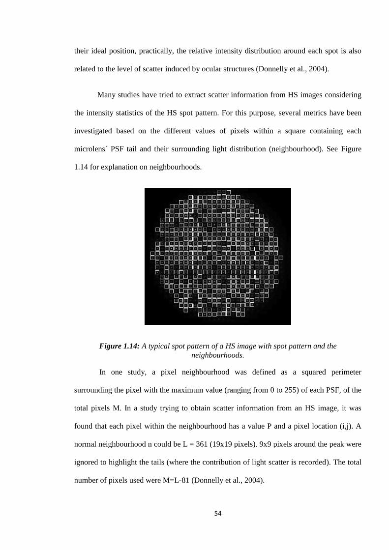
54

their ideal position, practically, the relative intensity distribution around each spot is also

related to the level of scatter induced by ocular structures (Donnelly et al., 2004).

Many studies have tried to extract scatter information from HS images considering

the intensity statistics of the HS spot pattern. For this purpose, several metrics have been

investigated based on the different values of pixels within a square containing each

microlens´ PSF tail and their surrounding light distribution (neighbourhood). See Figure

1.14 for explanation on neighbourhoods.

Figure 1.14: A typical spot pattern of a HS image with spot pattern and the

neighbourhoods.

In one study, a pixel neighbourhood was defined as a squared perimeter

surrounding the pixel with the maximum value (ranging from 0 to 255) of each PSF, of the

total pixels M. In a study trying to obtain scatter information from an HS image, it was

found that each pixel within the neighbourhood has a value P and a pixel location (i,j). A

normal neighbourhood n could be L = 361 (19x19 pixels). 9x9 pixels around the peak were

ignored to highlight the tails (where the contribution of light scatter is recorded). The total

number of pixels used were M=L-81 (Donnelly et al., 2004).

55

The influence of exposure time and the size of the pupil on a HS derived metric of

forward scatter was studied using a model of nuclear cataract (Donnelly and Applegate,

2005) concluding that the metric of MAX_SD (maximum standard deviation of the PSF

lenslets of a HS image) was the one which better explained the results obtained in the

study. With respect to the saturation of the HS images, the histograms were used to

identify saturated pixels. The image histogram plotted the number of pixels in the HS

image (after the removal of the background) against the pixel value. Saturated HS images

were observed in the histogram as a third peak near the value of 255 (non-saturated HS

images did not present it). It was concluded that to avoid saturation and maximize the

dynamic range of the system, the exposure time should be selected before the cataract

assessment (Donnelly and Applegate, 2005).

Light scatter from the analysis of the HS images (Figure 1.14) has also been

investigated in cataractous, keratoconic and normal eyes. In this study, two different

methods were used, the first one measured of the contrast of the HS image while the

second one measured the width of the PSF. Subsequently, the difference between the

measured contrast of the HS image and the widths of PSFs were computed and calculated

with the aid of an aberrometer. Twelve neighbourhoods around the centre of the pupil were

found to correspond to a pupil diameter of 4mm (Mihashi et al., 2006).

In 2009, Perez Sanchez defined a matrix in which each spot belonged to a small

square of 25 pixels of side. In each square, it was calculated a “local parameter” (LP)

through the division of the intensity registered in the periphery of the highest value of the

square by the intensity of an area of 9 pixels centred on the highest level of the square.

This LP provided the scatter of each small square within the HS image. To obtain a global

evaluation of the scatter in the plane of pupil, the scatter local parameters were calculated

56

for each square. The mean value of all of them was called “global scatter parameter” (GSP)

and included the normalization of the highest value of the LP. With this normalization, the

value of the GSP ranged from 0 to 10, following the expressions (Perez Sanchez, 2009):

i i i

i i i

Equation 1-3: Local parameter (LP) calculation (also called neighbourhoods) (Perez

Sanchez, 2009).

G

( )

Equation 1-4: Global scatter parameter (GSP) calculation (Perez Sanchez, 2009).

In addition to the value of GSP, the value of standard deviation associated with the

group of LPs provided information relative to the presence of local opacities within the

considered pupil diameter. For this reason, the standard deviation of each image was also

calculated (Perez Sanchez, 2009).

Finally, Cerviño et al. in 2008 also showed that Max_SD was a repeatable

parameter in human eyes. A correlation of 69% was found between the analysis of HS

images using Max_SD and the C-Quant straylight meter (Cerviño et al., 2008).

• The optical reconstruction of the wide –angle PSF in the living human eye (up to

8 degrees of eccentricity): This instrument (Ginis et al., 2012) based on a double pass

system projects a uniform disc of light into the retina. The recorded image from the retina

is the convolution of the initially presented disk and also contains information about the

PSF of the eye assessed. The dependency straylight – wavelength was found when

measuring small scatter angles while it was not possible to obtain same results for wide

scatter angle (Ginis et al., 2013). Figure 1.15 shows a scheme of the developed instrument.

57

Figure 1.15: Instrument for the reconstruction of the wide angle PSF in the human eye

(Ginis et al., 2013). In the figure, C is a condenser lens, D is diffuser, P is linear

polarizers, D1 and D2 diaphragms, LCWS is a liquid crystal selectable bandwidth tunable

optical filter, LC-SLM is a liquid crystal modulator and BS a beam splitter.

Basically, the bandwidth tunable optical filter (LCWS) selects different

wavelengths between 500 and 650nm and project a series of different discs (50) over the

retina. The radius of the ring ranged from 0.18 to 7.3 degrees of eccentricity. Then, the

image of the projected disc is compared to the double pass image recorded from the retina

and the increase of the intensity in the centre of the disc due to between the two images

recorded (Ginis et al., 2013).

1.9 RATIONALE

Currently, the most used instrument to obtain FLS measurements is the C-Quant

straylight meter. The measuring methodology used by this instrument is the compensation

comparison method (Franssen et al., 2006b), which is an evolution from the direct

compensation method (van den Berg and Ijspeert, 1992) and that is being widely used prior

58

to the introduction of C-Quant. However, the direct compensation method is still in use in

many laboratories but there is no existing comparison in the literature with its successor.

Some studies have attempted to obtain an objective FLS measurement from

commercially available instruments such as the Hartmann-Shack aberrometer, in which

FLS information can be extracted from the spot pattern images (Donnelly et al., 2004,

Cerviño et al., 2008, Perez Sanchez, 2009). These FLS measurements have been later

compared to BLS measurements ((Donnelly et al., 2004). However, the relationship

between the objectively measured BLS (through Scheimpflug imaging) and subjective FLS

in patients is not yet clear (Bueno et al., 2004, Donnelly et al., 2004).

Researchers have also developed instruments for the objective measurement of FLS

((Vilaseca et al., 2010, Ginis et al., 2012). Nonetheless, there is currently no methodology

that can relate FLS measurements with psychophysical data. In addition, the C-Quant

straylight meter is an instrument based on subjective measurements (based on subject´s

input) and designed to measure only wide-angle FLS (van den Berg et al., 2009a). An

instrument that could measure FLS at a range of scatter angles would be highly beneficial

for clinical diagnosis, considering that size and shape of the analysed particles with respect

to the wavelength of the incident light will affect their scattering behaviour: narrow or

wide angle scatter.

AIMS

The objectives of the present PhD project were to assess whether the FLS measured

through objective techniques correlate with the values obtained by the current subjective

gold standard instrument of assessing FLS (C-Quant straylight meter), and to develop an

objective technique for measuring FLS. More specifically, the project aimed to:

59

Compare the two most documented psychophysical techniques to assess FLS

(direct compensation and compensation comparison method) (chapter 2).

Improve the current understanding about the objective FLS information contained

on the Hartmanngrams (spot patterns obtained from the Hartmann-Shack

aberrometer) and check whether this information can be related to a subjective

measurement (C-Quant) (chapter 3).

Assess the relationship between an objective BLS measurement and a subjective

FLS measurement (chapter 4).

Develop an experimental optical set-up together with an eye model that measures

objectively FLS and can relate the values to psychophysical parameters (chapter 5).

60

2. COMPARISON OF THE COMPENSATION

COMPARISON METHOD AND THE

DIRECT COMPENSATION METHOD FOR

STRAYLIGHT MEASUREMENT

2.1 CONTRIBUTIONS

The study was designed by me and my supervisors, Hema Radhakrishnan and Vincent

Nourrit. The data collection was done by my supervisor Vincent Nourrit. The data analysis and the

writing of the study were done by me with support from the co-authors.

2.2 PUBLISHING OF THE PAPER

Authors for this study are Pablo Benito Lopez, Hema Radhakrishnan and Vincent Nourrit.

This paper will be submitted with the title: “Comparison of the compensation comparison method

and the direct compensation method for straylight measurement”. Target journal: Clinical and

Experimental Optometry. To be submitted.

2.3 PRESENTATION AT CONFERENCE

BENITO LOPEZ, P., RADHAKRISHNAN, H. & NOURRIT, V. 2014. Comparison of the

compensation comparison method and the direct compensation method for straylight

measurement. Proceedings of the VII European/ I World Meeting in Visual and Physiological Optics

VPOptics 2014.

61

2.4 ABSTRACT

PURPOSE: The van den Berg straylight meter was used to assess FLS in a large variety of

conditions and pathologies. Although still present in some research laboratories, it was

gradually replaced by the more robust C-Quant. The two instruments share similarities

(compensation comparison method for the first one, direct compensation method for the

second). The purpose of this article is to assess quantitatively the agreement between the

two techniques to facilitate comparison of clinical data obtained with each instrument.

DESIGN: Prospective study.

METHODS: FLS values were obtained from 35 subjects (ages ranging from 19 to 77)

with the C-Quant and the van den Berg Straylight meter (for each of the three different

eccentricities of the scattering source S=3.5⁰, M=10⁰, L =28⁰). Scatter values from both

instruments were then compared with two tailed paired sample t-test and Bland-Altman

plots. Pearson´s correlation coefficients, coefficients of agreement and limits of agreement

were calculated.

RESULTS: A weak linear correlation was found between the two instruments for the three

eccentricities (S: r2=0.13, p=.03; M: r

2=0.33, p<.001; L: r

2=0.36, p<.001). The coefficients

of agreement for the C-Quant and Straylight meter at each eccentricity were respectively:

S=0.58, M=0.49, L=0.49. The limits of agreement for each eccentricity were found to be a

large interval in comparison to the expected scatter value for a normal individual

(approximately 0.9).

CONCLUSIONS: Although C-Quant values are approximately of the same order of

magnitude as the straylight meter values, no direct equivalence can be made. Comparison

62

in a clinical study between C-Quant values obtained and previously published straylight

values should be done carefully.

2.5 INTRODUCTION

In the last decade, a growing number of papers focused on the assessment and

consequences of intraocular Forward Light Scattering (FLS) have been published (see the review

papers: (Pinero et al., 2010, van den Berg et al., 2013)). Forward light scattering (FLS) occurs when

part of the light propagating through the eye is deviated (scattered) from its original path by less

than 90 degrees and does not participate towards the formation of the image. This scattering may

induce discomfort or disability glare which can significantly affect the visual performances and

quality of life of the patient (de Waard et al., 1992).

FLS is by definition intrinsically difficult to assess objectively and quantitatively and does

not correlate well with backward light scatter (Donnelly Iii et al., 2004, Rozema et al., 2011). In this

context, the van den Berg Straylight meter (VDB, Observator BV, Ridderkirk, The Netherlands) (van

den Berg and Ijspeert, 1992) has been long considered the gold standard to assess FLS and to

quantify the discriminative ability, reliability and validity of various glare tests (Elliott and

Bullimore, 1993). This instrument was used to quantify FLS in a large variety of clinical conditions,

including patients with cataracts (de Waard et al., 1992) and associated posterior capsule

opacification (Meacock et al., 2003), but also corneal oedema (Elliott et al., 1993) and corneal

dystrophies (Van den Berg et al., 1994, Patel et al., 2008a, Patel et al., 2008b), retinal disorders

(Grover et al., 1998), keratoconus (Jinabhai et al., 2012), hypopigmentation (van den Berg and H,

1986), refractive surgery (Veraart et al., 1995), corneal grafts (Patel et al., 2008a, Patel et al.,

2008b), or in association with contact lenses (Elliott et al., 1991).

63

Relatively recently, an improved version of this instrument, the C-quant (Oculus

Optikgerate Gmbh, Wetzlar, Germany) (Franssen et al., 2006) has been introduced. This new

instrument is easier to use in practice (Cerviño et al., 2008, van den Berg et al., 2013) and based

on a more robust approach, the compensation comparison method (Coppens et al., 2006). This

method improves repeatability and reliability of the measurement (Coopens et al., 2006, Coppens

et al., 2006, Cervino et al., 2008, Cerviño et al., 2008) with respect to the Straylight meter. No

reports however can be found in the literature about the correlation between the straylight

parameter produced by the C-Quant and the three values obtained with the straylight meter

(associated to 3 different glare source eccentricities). Since numerous studies reported straylight

measurements in a large variety of conditions and pathologies with the Straylight meter, and since

it is still used in some research laboratories, our aim is to assess quantitatively the agreement

between the two techniques.

2.6 METHODS

PARTICIPANTS

Thirty five healthy subjects aged from 19 to 77 (41.6±21.7 [mean±SD]) years old

were recruited from the student and staff populations of the University of Manchester.

Young and older participants were studied as a single group to obtain data reflecting a

broad spectrum of straylight value. Contact lens wearers were not included in the study.

Any history of ocular disease or ocular pathology was considered as exclusion criteria.

This study followed the tenets of the Declaration of Helsinki and was approved by the

research ethics committee of the University of Manchester (UK). Informed consent was

obtained from all participants after the nature and possible consequences of the study were

explained.

64

FLS values from all subjects were measured monocularly in both eyes. However,

only data obtained from the right eye was considered for calculations (Ray and O'Day,

1985).

VDB STRAYLIGHT METER

The basics of the Straylight meter are the following. The patient looks into a tube to

observe a ring of flickering (8Hz) light-emitting diodes (LEDs) with a wavelength of

570±30nm. The image of the ring is formed on the retina of the patient, and, in the case of

a perfect eye, this image would be sharp and there would not be any light in the centre of

the ring. In the presence of scatter, some light will be scattered in the middle of the imaged

ring. Consequently, the amount of light in the centre of the imaged ring is directly

proportional to the intraocular scatter. Since the ring can be equated to a small source of

eccentricity θ, the use of various rings allows measurement of the angular dependence of

the intraocular scatter (see Figure 2.1). In practice, there is also a spot source in the centre

of the ring and the two sources (spot+ring) are flickering in counter-phase. The task of the

observer is to adjust the luminance of the spot to cancel the flickering, i.e. to match the

veiling illuminance produced by the scattered light. For this reason, this technique is

referred to as „direct compensation‟.

Six measurements were taken in total for each participant, two measurements for

every eccentricity of the scatter source (3.5°, 10° and 28°) (van den Berg and Ijspeert,

1992). Measurements for each one of the eccentricities were averaged. Subjects with

refractive correction were measured with their habitual spectacles. The spectacles

transparency was assessed before measurement (clean, no scratches that might affect the

measurement (De Wit and Coppens, 2003)).

65

C-QUANT

The compensation comparison method used by the C-Quant straylight meter

(Franssen et al., 2006) is similar to the direct compensation technique. However, in this

case, the inner test field is divided into two flickering half-discs inside of another flickering

ring. The ring represents the glare source (achromatic light) and has an effective angle of 7

degrees of eccentricity (van den Berg, 1995). The psychophysical test consists of series of

2-forced choice test where the participant has to decide which one of the two half discs is

flickering the most (see Figure 2.1). The psychometric function used by this method

(Franssen et al., 2007) decides which comparisons are shown to the participant. The test

provides a measurement of the FLS, the standard deviation of the measure (ESD) and a

quality factor of the psychometric function (Q) (Coopens et al., 2006). Reliability of the

measurements is considered acceptable when ESD is lower than 0.08 and Q higher than 1.

Figure 2.1: Van den Berg straylight meter and C-Quant straylight meter. The van den

Berg straylight meter has three different glare sources to measure at 3.5, 10 and 28

degrees of eccentricity while the C-Quant straylight meter has only one at 7⁰ of effective

eccentricity. Glare sources in both instruments have a flickering frequency of 8Hz. In the

van den Berg straylight meter the testing field is a central disc while C-Quant has a circle

with two testing halves. C-Quant straylight meter uses a achromatic light while van den

Berg straylight meter uses LEDs of 570±30nm.

66

The measurements were obtained in scotopic light conditions after the correct

positioning of the participant with respect to the instrument was checked (van den Berg,

2014). The test was repeated until two reliable measurements were obtained (ESD<0.08

and Q>1). The instrument allows inserting lenses to correct for the refractive error

(spherical equivalent) of the subject so subjects did not have to wear their spectacles (van

den Berg, 2014).

DATA ANALYSIS

The distribution of the data was analysed with the Kolmogorov-Smirnov test for

normality. Relations between C-Quant measurements and Straylight meter values for each

one of the eccentricities (S, M and L) are assessed with two tailed paired sample t-test and

Pearson‟s correlation coefficient (r), considering a p-value less than 0.05 as significant.

The relations between instruments values were determined with Bland-Altman

plots (Bland and Altman, 1986, Bland and Altman, 1999) and the coefficient of agreement

(COA) obtained for each two sets of data compared. In the present study, limits of

agreement were calculated as the mean value of the differences between the two methods ±

1.96 times the standard deviation of the differences between two sets of measurements (C-

Quant and one of the Straylight meter eccentricities (S, M or L)). It represents the interval

where the differences in measurements from 2 instruments can be expected to fall with

95% probability (Bland and Altman, 1986).

A multiple regression analysis was performed in order to assess the relationship

between C-Quant values (dependent variable) and the three eccentricities measured with

the Straylight meter S, M and L (independent variables). The absence of multicollinearity

is one of the assumptions to perform a multiple regression analysis. In this sense,

67

correlation coefficients (r) between variables (C-Quant, Straylight meter S, M and L) and

Variance Inflation Factor (VIF) were calculated. The multiple regression analysis is

considered viable when the correlation coefficients relating dependent with independent

variables are preferably be above 0.3 while relationship between independent variables are

not too high (normally less than 0.9). VIF, as an indicator of multicollinearity, it explains

how much the independent variables of a multiple regression are linearly related. A VIF

value higher than 10 was considered as an indication of multicollinearity (Pallant, 2010).

The results of this analysis were obtained using SPSS Statistics 21 (IBM, Chicago,

IL) and MedCalc 12 (MedCalc Software, Mariakerke, Belgium).

2.7 RESULTS

The data summarised in Table 2.1 represents the values obtained with the C-Quant

and the three different eccentricities of the Straylight meter (S = 3.5⁰, M = 10⁰ and L =

28⁰). It is appreciable that mean straylight values obtained from the Straylight meter

decrease as the measured scatter angle increases (S = 1.12, M = 1.04 and L = 0.99). This

tendency has been previously reported (Jinabhai et al., 2012).

C-

Quant

(Log(s))

Straylight meter (log(s))

S M L

Mean 1.08 1.12 1.04 0.99

SD 0.29 0.22 0.24 0.25

Min 0.72 0.62 0.58 0.51

Max 1.93 1.62 1.69 1.45 Table 2.1: Summary of the mean values, standard deviation (SD), minimum and maximum

values obtained for C-Quant and the 3 different eccentricities of Straylight meter (S, M, L).

68

The data distributions obtained from the study and assessed with the Kolmogorov-

Smirnov test were found to be normal for C-Quant (p > 0.10), Straylight meter (S) (p >

0.10), Straylight meter (M) (p > 0.10) and Straylight meter (L) (p > 0.10). Boxplot of the

distribution of data is presented in Figure 2.2.

Figure 2.2: Boxplot diagram representing the distribution of data for C-Quant and the

three Straylight meter eccentricities measured (S, M and L). Boxes contain 50% of the data

(from lower to upper quartile) while the line inside represents the median value. Vertical

lines cover from the minimum to the maximum value, excluding the outside values (circles)

and the far out values (black squares).

In Figure 2.3, the Straylight meter values for the three different eccentricities (S, M

and L) are plotted against the C-Quant (CQ) values. Pearson´s correlation coefficient for

each pair of data set showed a weak linear relationship between FLS values obtained with

the two instruments (r2

= 0.13 and p = 0.03 for Straylight meter(S) and C-Quant, r2

= 0.33

and p < 0.001 for Straylight meter(M) and C-Quant, r2

= 0.34 and p < 0.001 for Straylight

meter(L) and C-Quant). T-tests results for C-Quant and each one of the eccentricities S, M

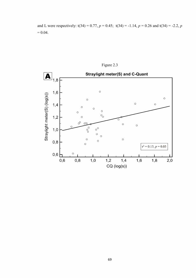
69

and L were respectively: t(34) = 0.77, p = 0.45; t(34) = -1.14, p = 0.26 and t(34) = -2.2, p

= 0.04.

Figure 2.3

70

Figure 2.3: Scatter value from C-Quant is plotted against the three different tested

eccentricities (S = 3.5⁰, M = 10⁰, L = 28⁰) of the Straylight meter (A = Straylight meter(S)

and C-Quant, B = Straylight meter (M) and C-Quant, C = Straylight meter for L is plotted

against the mean CQ). Pearson´s correlation coefficient and p value are shown on the

graphs. A weak relationship can be observed between values obtained from both

instruments.

71

In order to gain a better understanding of the relation between the C-Quant and

Straylight meter data sets, the associated Bland-Altman plots (difference C-Quant-

straylight results plotted against the associated mean) are represented in Figure 2.4. The

spread of the data representing differences of the values between the two instruments with

respect to the mean does not show any direct relationship between the two instruments for

each one of the eccentricities.

Figure 2.4

72

Figure 2.4: The graphs show the differencies of the measurements between the two

methods plotted against their mean values for each one of the three different tested

eccentricities (A: S=3.5⁰, B: M=10⁰, C: L=28⁰). Mean value of the differences and limits

of agreement (defined as mean of the differences ± 1.96xSD) are also presented.

73

Table 2.2 shows the statistics obtained for the differences of C-Quant values and the

three eccentricities measured with the Straylight meter.

S-CQ M-CQ L-CQ

Mean 0.04 -0.05 -0.09

Standard Deviation 0.29 0.25 0.25

Min -0.54 -0.54 -0.58

Max 0.62 0.44 0.4

COA 0.58 0.49 0.49

Limit of agreement Max 0.62 0.44 0.40

Limit of agreement min -0.54 -0.54 -0.58

Table 2.2: Statistics for the differences of C-Quant (CQ) values minus straylight data for

each one of the three eccentricities of the Straylight meter (S-CQ, M-CQ, L-CQ) including

the Coefficients of agreement (COA).

To perform the multiple regression analysis, multicollinearity is assessed. Table 2.3

shows the correlation coefficients (r) relating the four variables (C-Quant and eccentricities

S, M and L of the Straylight meter).

VARIABLE C-Quant Straylight meter S Straylight meter M

Straylight meter S 0.37

Straylight meter M 0.57 0.78

Straylight meter L 0.58 0.66 0.82 Table 2.3: Correlation coefficients (r) relating C-Quant values and the three eccentricities

measured with the Straylight meter (S, M and L).

To calculate VIF, linear relationship between independent variables is evaluated

while another variable acts as dependent one. To do this, each one of the variables (C-

Quant value, Straylight meter S, M and L) will act as dependent variable while VIF is

calculated for the remaining three variables. This process is repeated as many times as

variables are evaluated (four in this case). Table 2.4 shows the results of this analysis. VIF

74

values lower than 10 indicate the absence of multicollinearity and the viability of the

multiple regression analysis.

DEPENDENT VARIABLE

CQ S M L

INDEPENDENT VARIABLES

S M L CQ M L CQ S L CQ S M

VIF 2.56 4.52 3.15 1.56 3.28 3.33 1.5 1.78 2.31 1.52 2.61 3.35

Table 2.4: Calculation of VIF for the variables C-Quant (CQ) and the three eccentricities

of the Straylight meter S, M, and L.

The multiple regression analysis is depicted in Table 2.5. In this analysis, the

dependent variable is C-Quant while the three eccentricities of the Straylight meter act as

independent variables. The coefficient of determination R2 obtained for this analysis

reveals that independent variables (three eccentricities measured with the Straylight meter)

explain the 38.03% of the dependent variable (C-Quant straylight value). However, this

result cannot be considered statistically significant (p=.0018) as p value for the calculation

of R2

should be less than 0.001. Coefficients obtained for each one of the independent

variables analysed showed an influence over the dependent variable (C-Quant) with -0.28

for Straylight S, 0.54 for M and 0.41 in case L. However, as with the coefficient of

determination, none of the coefficients obtained for the independent variables are

statistically significant (p > 0.05 for a 95% confidence interval).

INDEPENDENT VARIABLES COEFFICIENTS STD.

ERROR t-value

p-value

Constant 0.43

Straylight meter S -0.28 0.3 -0.95 0.35

Straylight meter M 0.54 0.36 1.49 0.15

Straylight meter L 0.41 0.3 1.39 0.17 Table 2.5: Multiple regression analysis using C-Quant as dependent variable and the three

eccentricities of the Straylight meter as independent variables. Coefficients, standard error

(Std. Error), t-value and correspondent p-value are also shown.

75

2.8 DISCUSSION

The aim of the present study was to assess the agreement between the direct

compensation (van den Berg Straylight meter) and the compensation comparison technique

(C-Quant). Both techniques have been proven useful. While the Straylight meter was the

gold standard for several years in techniques to assess FLS and led to many publications

(Elliott and Bullimore, 1993, Veraart et al., 1995, Jinabhai et al., 2012) the C-Quant has

probably replaced it as the most used instrument to measure FLS (Van Den Berg et al.,

2007, Nischler et al., 2010, Montenegro et al., 2012).

The results from this study are in agreement with straylight values published in the

literature for both van den Berg straylight meter (Jinabhai et al., 2012) and C-Quant (van

den Berg et al., 2013). However, the correlation between the straylight meter and the C-

Quant was shown to be weak for each eccentricity, particularly for the lowest eccentricity

(3.5deg r2

= 0.13, p < 0.03; 10deg; r2

= 0.33, p < 0.01; 28deg; r2

= 0.34, p < 0.01).

Theoretically a higher correlation with ring M should have been obtained but this can be

explained by the limited number of subjects and the variability of the measure.

However, further data analysis suggests that the values obtained with the two

instruments are not directly interchangeable. The limits of agreement for each eccentricity

were respectively equal to or larger than 0.49 (Table 2.2). This means that for a given

measurement with the C-Quant, the interval where we can expect the straylight meter value

to fall is too large to be clinically useful (e.g. for the M eccentricity, straylight meter ‟s

results should be -0.54 smaller or +0.44 greater than the C-Quant value (Table 2.2)).

Absence of multicollinearity between the four variables (C-quant, Straylight meter

S, M and L) indicates the viability of the multiple regression analysis. To perform a

multiple regression analysis, ccorrelation coefficients (r) relating the four variables need to

76

be above 0.3 and below 0.9 and VIF (Table 2.4) values lower than 10 (Pallant, 2010).

However, the coefficient of determination (R2) and coefficients obtained for each one of

the predicting variables (Table 2.5) were not statistically significant (p > 0.001 and p >

0.05 respectively). Hence, C-Quant straylight values cannot be predicted as a contribution

of the straylight values obtained with the Straylight meter for the three different

eccentricities measured (S, M and L). These results were not expected as the C-Quant

straylight value is proportional to the square of the angle measured (van den Berg et al.,

2013) and the distribution of scattered light over the retina. This lack of linear relationship

between C-Quant values and Straylight meter (S, M or L eccentricity values) might be due

to the different measured eccentricities in the van den Berg Straylight meter (3.5º, 10º and

28º) and C-Quant (7º), and leads us to think that straylight values obtained from C-Quant

should possibly be compared to a combination of the straylight values obtained for

different Straylight meter eccentricities. In this sense, the straylight produced by a glare

source of 7º of eccentricity (C-Quant) was supposed to be comparable to a combination of

the straylight produced by the three eccentricities (3.5º, 10º and 28º) of the Straylight

meter, or at least two of them (e.g. S = 3.5º and M = 10º).

The differences between the measurements obtained using the two techniques may

be due to a variety of factors. Firstly, the use of the psychometric function in C-Quant

provides the measurement with a reliability (Coopens et al., 2006) that is not available in

the van den Berg straylight meter. Secondly, the eccentricity of the glare source is not

strictly identical (3.5, 10 and 28 degrees for the Straylight meter (van den Berg and

Ijspeert, 1992) and 7 degrees for the C-Quant (van den Berg, 1995)) but also the type of

glare source used also varies. The Straylight meter is based on a ring of LEDs when the C-

Quant uses two half discs and a ring. Perhaps more importantly, both instruments rely on a

subjective estimation of scattering and the measured values cover slightly different ranges.

77

As a result, the standard deviation of the difference between the two measurements is

increased which can negatively affect the agreement between the two methods. This is

particularly true for the straylight meter which does not benefit from the improvements

present on the C-Quant (computerized 2-choices forced tests, measure of reliability).

As a conclusion, although C-Quant values are approximately of the same order of

magnitude as the straylight meter ones, no direct equivalence can be made. Comparison in

a clinical study between C-Quant values obtained and previously published straylight

values should be done carefully.

78

3. COMPARISON OF FORWARD LIGHT

SCATTER ESTIMATIONS USING

HARTMANN - SHACK SPOT PATTERNS

AND C-QUANT

3.1 CONTRIBUTIONS

The study was designed with the help of my co-authors. Both co-authors Hema

Radhakrishnan and Vincent Nourrit provided important contributions to the study. The data

collection and the writing of the study were done by me with useful advice from the co-

authors.


BENITO LOPEZ, P., RADHAKRISHNAN, H. & NOURRIT, V. 2015. Comparison of

forward light scatter estimations using Shack-Hartmann spot patterns and a straylight

meter. J Cataract Refract Surg, 41, 320-6. In-Press.


This research was presented in part as a paper presentation at the 6th EOS Topical

Meeting on Visual and Physiological Optics (EMVPO 2012). Held at University College

Dublin (UCD), Dublin, Ireland (20 August 2012 - 22 August 2012).

79

3.4 ABSTRACT

PURPOSE: To assess if a non-modified commercial wave front sensor can be used to

estimate forward light scatter and how this assessment matches the one obtained from

C-Quant.

DESIGN: Prospective comparative study between measurements obtained with C-Quant

and Hartmann-Shack (HS).

METHODS: Objective scatter data were derived using an HS metric based on previously

reported methodology. The method was first validated using a model eye, by spraying an

aerosol over 4 contact lenses to generate various levels of scatter. Measurements with

both methods (HS-based and C-Quant) were subsequently obtained in 33 healthy

participants (mean age of 38.9 ± 13.1 years).

RESULTS: A good correlation was observed (r = 0.97, p < 0.05) between the density of

droplets over the contact lenses and the objective scatter value extracted from the

hartmanngrams. The mean C-Quant values for participants were in agreement with those

reported in the literature for healthy subjects (0.87±0.18 [mean±SD]). However, no

significant relationship was found between the measurements obtained from C-Quant

and the metric derived from HS (r = 0.13, p = 0.46).

CONCLUSIONS: Although the hartmanngrams were found to provide a valid objective

measurement of the light scatter from model eyes, the measurements on human eyes

were not significantly correlated with the subjective and clinically accepted C-Quant light

scatter meter. The difference could be caused by the fact that C-Quant assesses large

80

angle scatter while HS method collates information from a narrow angle around the

centre of the point spread function.

3.5 INTRODUCTION

Intraocular light scatter occurs when the light passing through the ocular media

suffers a deviation from its original trajectory due to the presence of inhomogeneities in

the optical media (e.g. corneal scarring or cataract). In contrast to backward light scatter,

forward light scatter (FLS) reaches the retina. Its influence on the retinal image can be

equated to a superimposed veiling luminance (Fry and Alpern, 1953) and its main effect is

the impairing of the functional visual performances (i.e. reduced contrast sensitivity and

glare (Paulsson and Sjostrand, 1980, De Waard et al., 1992, Artal et al., 2001)). Recent

studies have suggested the use of intraocular light scatter as an additional test for

patients undergoing cataract surgery (Bal et al., 2011) or refractive surgery, particularly if

they have visually demanding professions (Van Bree et al., 2011).

The measurement of intraocular FLS is a difficult but important issue. Since the

beginning of the 20th century (Holladay, 1926, Stiles and Crawford, 1937), numerous

methods have been suggested for assessing FLS. Instruments to measure intraocular

scatter can be divided into two broad categories (subjective and objective) depending on

whether they rely on the patients’ input.

Several types of subjective methods have been developed (cf. Van Den Berg et al.

(van den Berg et al., 2012) for a recent survey of ocular straylight measurement). While

some techniques compare contrast sensitivity measurements in the presence and

81

absence of a glare source (Miller et al., 1972, Vaegan and Halliday, 1982, Bailey and

Bullimore, 1991, Van Den Berg, 1991, Elliott and Bullimore, 1993), perhaps the most

studied and documented instrument (C-Quant straylight meter, Oculus GmbH, Wetzlar,

Germany) uses the compensation comparison method (Franssen et al., 2006). It was

developed to diagnose patients with large angle light scatter in the eye (e.g. in patients

with early cataract) (Franssen et al., 2006). The C-Quant has good reliability and

repeatability for assessing FLS (Cervino et al., 2008). In addition, C-Quant has also been

successful in providing good correlation between measurements of FLS and reduction of

visual function (Van Den Berg et al., 2007, Michael et al., 2009).

The optical quality of the eyes is usually only described in terms of aberrations,

although the uniformity of the ocular media also affects the retinal image. Retinal image

and quality of vision (in part) can be explained and assessed qualitatively by the retinal

point spread function (PSF) (Montés-Micó et al., 2008, Van Den Berg et al., 2009). For this

reason, instruments providing objective measurements of FLS are usually based on the

double pass (DP) technique (analysing the light reflected by the retina) (Santamaría et al.,

1987, Artal et al., 1995, Kuroda et al., 2002, Donnelly Iii et al., 2004). Since Hartmann-

Shack wavefront sensors record an array of PSFs, several authors have suggested

different approaches for the extraction of light scatter values from the hartmanngrams

(Applegate RA, 2000, Kuroda et al., 2002, Applegate RA, 2003). The displacement of PSF

spots on the hartmanngrams is due to aberrations and the scatter value is retrieved by

calculating the intensity of PSF’s tails (Applegate RA, 2000, Donnelly Iii et al., 2004). Using

this method, Donnelly et al. (Donnelly Iii et al., 2004) evaluated five different metrics

referred to the intensity around the centre of each PSF of the hartmanngrams (PSFlet).

82

The maximum standard deviation of the intensities of each PSFlet of the hartmanngram

was found as the best metric explaining FLS (Donnelly Iii et al., 2004).

As several wavefront sensors have been developed for applications in

ophthalmology and optometry, the development of a numerical tool that can extract a

measure of FLS from the analysis of the hartmanngrams could extend the range of

applications of commercial wavefront sensors. However, this method has been reported

mainly with research instruments and without any comparison to any results obtained by

a subjective technique. Only one study addressed this issue but with a limited number of

measurements (Cerviño et al., 2008). For this reason, the aim of this study is to assess if a

non-modified commercial wave front sensor could be used to estimate FLS (via the

development of a numerical tool) and how this assessment would match the one

obtained with a method sometimes considered as the gold standard (C-Quant straylight

meter).

3.6 METHODS

This study is comprised of two experiments:

1. Measurement of FLS with customized contact lenses: Six customized contact

lenses with different amounts of scatter were placed in front of a model eye. After

obtaining the hartmanngram from both contact lens + model eye, a mathematical

algorithm extracts the scatter value from it.

83

2. Measurement in subjects with both HS and C-Quant: After validating the

algorithm to extract the scatter value from the hartmanngrams, measurements

from thirty three subjects are obtained from both Hartmann-Shack and C-Quant,

thus comparing, objective with subjective measurements of FLS respectively.

MEASUREMENT OF FLS FROM THE HS IMAGES

The irx3 wavefront sensor (see Figure 3.1 for information about HS sensors) uses

the HS technique with an infrared light of 780nm to measure aberrations and a lenslet

array of 32x32.









consequence of diffraction, aberrations and light scatter.

84

The array of lenslets produces the hartmanngram spot pattern (Figure 3.2A). In

such an image, the displacement of the spots with respect to their reference position is

due to the aberrations. The width of each spot (or PSFlet) is related to FLS (Figure 3.2B).

The lenslet and detector properties of the irx3 wavefront sensor are not publicly available

and it is thus difficult to provide an exact value of the pixel size in minutes of arc.

However, according to previous publications (e.g. Leroux et al. (Leroux and Dainty, 2010)

and Nam et al. (Nam et al., 2011)) a value around 3 arcminutes could be expected).

85

Figure 3.2: A) Hartmanngram spot pattern from one of the participants. In this picture,

each square represents an area of 13x13 pixels around the centroid; squares containing

more than two saturated points or whose intensity pixels were under the threshold

(obtained to analyse the images with Matlab) were not considered for calculations and

look missing. For this particular hartmanngram, the mean, standard deviation, minimum

and maximum of the standard deviations of all PSFlets were respectively 8.9x10-3

,

6.87x10-2

, 7.7x10-3

, 0.17. The associated HS value is equal to the maximum standard

deviation. B) An enlarged PSFlet showing the centre of the PSF and the surrounding

intensity. The sampling distance in the pupil plane is 0.23mm.

A custom written Matlab (MathWorks®, Natick, MA) program (program code is

available in the Annexes of this thesis) was developed to extract the scatter information

from the HS images following the approach described by Donnelly et al. (Donnelly Iii et

al., 2004) The Matlab program included the following steps:

Rejection of images of poor quality (defocused, highly irregular spots pattern due

to blinking or poor centration).

Rejection of overexposed images. Due to the short dynamic range of the HS CCD

camera (8 bits), HS images are easily overexposed. Overexposed images are

86

difficult to analyse, as information around the centre of the PSFlet is lost by

clipping. To avoid this problem, images where image histogram showed a third

peak were considered overexposed and removed from calculations (Donnelly Iii

and Applegate, 2005). In addition, some of the PSFlet may present local

saturation. It was considered that PSFlets with more than 2 saturated pixels i.e.

pixel value of 255 (the maximum value possible to be recorded on the HS sensor),

do not contribute to the scatter calculations for the whole image.

Extracting a metric for FLS from the Hartmanngrams: Hartmanngrams from the HS

are converted into an intensity image. To reduce noise (fluctuation in the signal

produced by all electronic instruments) the lowest intensity value of the image is

subtracted to all pixel values of the hartmanngram. Subsequently, the intensity

image is thresholded to find the location of the centroids of each PSFlet and to

index them. Thresholding of the images was done empirically in order to assess

the lowest intensity pixels of the neighbourhoods (most information on FLS within

the neighbourhood is stored near the borders of the neighbourhood, where

intensity pixels are lower) after removing the noise of the image. A 13x13 pixel

neighbourhood is defined around each centroid. PSFlets with very low intensity

values with respect to the threshold or those with more than two saturated points

are not considered for calculations. Finally, the standard deviation of the pixel

intensities from each PSFlet of the Hartmanngram is calculated and the maximum

one is used as a measure of scatter. This is the metric suggested by Donnelly et al.

(Donnelly Iii et al., 2004) and used in Cerviño et al. (Cerviño et al., 2008).

87

EXPERIMENT 1: MEASUREMENT OF FLS WITH CUSTOMIZED CONTACT LENSES

In order to validate this program, measurements were obtained with a model eye

(RME - http://www.optomshop.co.uk/Retinoscopy_Model_Eye.htm, January 2013). To

simulate different levels of scatter, different concentrations of aerosol containing

aluminium chlorohydrate (refractive index = 1.51) were sprayed over six RPG contact

lenses (Figure 3.3). The lenses were sprayed for approximately 0 (none), 0.5, 1 and 1.5

seconds at a distance of 40 centimetres. The concentration of the aerosol particles was

then measured by obtaining an image of the central zone of each lens (representing 60%

of the whole lens area) and processing it with Matlab to estimate the droplets’ density.

Images of the lenses 1 hour after spraying were also taken to assess that the density and

opacity of the droplets over the lenses remained stable.

To measure the magnitude of light scatter, the model eye was collocated in front

of the aberrometer with clamps. The end of the model eye was covered with a black

rough surface to reduce the amount of light reflected and to avoid overexposing the HS

sensor. The recording of the hartmanngrams was executed in scotopic light (less than 0.5

lux), changing only the lens holder with the contact lens in front of the model eye and

leaving the rest of the set-up steady. The HS images were obtained for the non-sprayed

lenses first and then the lenses were changed in incremental order with the most sprayed

lenses being tested in the end. Three hartmanngrams were recorded, processed and

averaged for each contact lens per level of scatter. Therefore, there were 12 images in

total, obtained with the HS sensor for each lens. The whole process was repeated for all

the six lenses.

http://www.optomshop.co.uk/Retinoscopy_Model_Eye.htm

88

Figure 3.3: Photos of one 9mm RPG contact lens (left) for each density of aerosol droplets

(simulating different scatter conditions). Right: photo of the central zone of the lens (60%

of the lens = 38.06mm2) after processing with Matlab to assess objectively the droplets

density. First line of photos shows the non-sprayed lens. Consecutive lines correspond to

same lens with added quantities of spray (without removing the previous spraying). Pixel

size of the photos (obtained with a normal camera) is 1.4 microns and the mean droplet’s

size was 31.2 ± 21.52 pixels.

89

EXPERIMENT 2: MEASUREMENTS IN SUBJECTS WITH BOTH HS AND C-

QUANT

Thirty three subjects took part in the study after providing informed consent. The

study was approved by the University of Manchester Research Ethics Committee. The

mean and standard deviation of our patients’ age was 38.9 ± 13.1 years with the

minimum and maximum age being respectively 24 and 62 years. Mean spherical

equivalent was -1.22 diopters ± 3.07 SD (max = 6.75, min = -9.00). Pupil size of each

participant was measured in the dark (6.29±0.61mm (mean±SD); min= 5mm;

max=6.8mm) and set mechanically to 5 mm with the Hartmann-Shack aberrometer. The

criteria of exclusion were the following: ocular pathology, history of ocular diseases, and

contact lens wear in the last 24 hours. Subjects wearing glasses (17) were measured

without them on both instruments, using lenses for the correction of refraction (spherical

equivalent) in case of C-Quant (Van Den Berg, 2014). Participants were selected from a

relatively wide range of age groups so that the data would span a broad range of

straylight values (Hennelly et al., 1998).

The measurement technique with the C-Quant (Oculus) has been described by

Franssen et al. (Donnelly Iii and Applegate, 2005). In summary, the subject looks into a

tube at two flickering half-discs, surrounded by a flickering annulus simulating a glare

source of achromatic light at 7 degrees of eccentricity. The test consists of approximately

20 forced choices where the subject has to decide which half-disc is flickering the most.

At the end of the test, one measure of straylight is produced, together with the standard

deviation of this measure (ESD) and a quality factor (Q). Measurements can be considered

reliable when the ESD is lower than 0.08 and the quality factor higher than 1. Monocular

measurements were taken in scotopic light conditions. The correct position of the patient

90

was also carefully monitored as it may influence the measurement (Van Den Berg, 2014).

Two measures were taken for each eye. If both measures were reliable, the mean value

of these 2 measures was taken as the scatter log value; if not, the measurement was

repeated until 2 acceptable measurements were obtained (ESD<0.08, Q>1) where ESD is

the estimated standard deviation and Q is the fit quality parameter of the psychometric

function (Coopens et al., 2006).

The irx3TM wavefront sensor was used to obtain the HS images. Three

measurements were obtained for each eye of the patient in scotopic light conditions. If

any of the images was thought not to be valid (e.g. blinking), a new one was taken. The

test was done on each eye monocularly, without refractive corrections and using an

occluder to cover the non-tested eye.

STATISTICAL ANALYSIS

The Pearson’s correlation coefficient (r) and two tailed paired sample t-test are

obtained to find an association in both experiments. Data sets were checked for normality

using the Kolmogorov-Smirnov test and a p-value lower than 0.05 was considered

significant.



91

3.7 RESULTS


Figure 3.4 shows the FLS values extracted from the hartmanngrams of the

customized contact lenses in comparison with the calculated density of droplets over the

same lenses (cf. Methods). Figure 3.4 illustrates a significant correlation between the two

sets of data (r = 0.97, P < 0.05).

Figure 3.4: Relationship between the amount of FLS for each lens (extracted from the

hartmanngrams) and the associated concentration of scatter droplets.

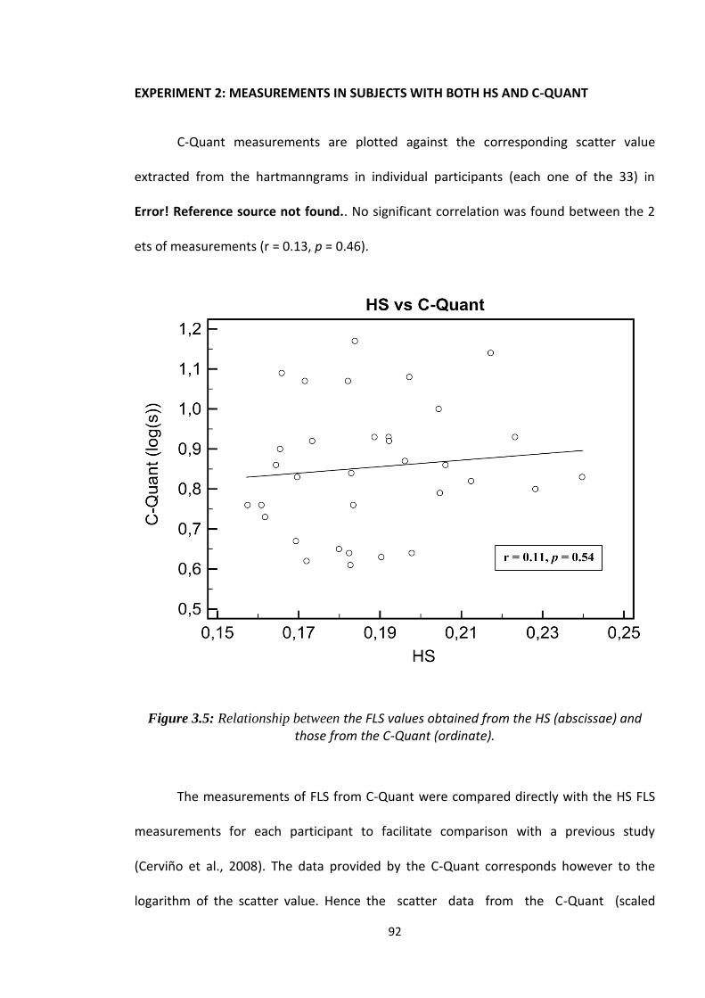
92

EXPERIMENT 2: MEASUREMENTS IN SUBJECTS WITH BOTH HS AND C-QUANT

C-Quant measurements are plotted against the corresponding scatter value

extracted from the hartmanngrams in individual participants (each one of the 33) in

Error! Reference source not found.. No significant correlation was found between the 2

ets of measurements (r = 0.13, p = 0.46).

Figure 3.5: Relationship between the FLS values obtained from the HS (abscissae) and those from the C-Quant (ordinate).

The measurements of FLS from C-Quant were compared directly with the HS FLS

measurements for each participant to facilitate comparison with a previous study

(Cerviño et al., 2008). The data provided by the C-Quant corresponds however to the

logarithm of the scatter value. Hence the scatter data from the C-Quant (scaled

93

linearly) was compared to the HS data. No significant correlation was found (r = 0.11,

p = 0.53).

3.8 DISCUSSION


The results from this experiment agree with those obtained in a previous study

(De Brouwere, 2007) in which different concentrations of microspheres with variable

diameter and known refractive index were used to simulate increased corneal scatter.

The study (De Brouwere, 2007) used a commercial wavefront analyser (WaveLight

Wavefront Analyser, WaveLight Technologie Inc., Erlangen AG) and the results showed an

increased scatter as the concentration of microspheres became higher. The use of

microspheres in contact lenses to simulate corneal scatter was validated and found

reliable for the comparison and calibration of optical devices measuring ocular scatter. In

this study, using an artificial eye and six contact lenses with pre-determined amount of

droplets containing aluminium chlorohydrate, the irx3TM Wavefront Aberrometer

returned proportionally higher scatter values as concentration raised.

EXPERIMENT 2: MEASUREMENTS IN SUBJECTS WITH BOTH HS AND C-QUANT

The lack of correlation observed between the CQ data and the one estimated from

the HS spot patterns can be at first surprising. However, it can be explained by different

factors. Firstly, both instruments are intrinsically different in design and objectives. The C-

94

Quant is mainly sensitive to large angle scatter while HS measures a very narrow angle

scatter around the centre of the PSF (Van Den Berg et al., 2009). This large dimensional

difference in angular domain could be related to different physical processes. The PSFlet

spread may be related to irregularities causing "micro-aberrations" (Nam et al., 2011) (i.e.

aberrations on a spatial scale less than the diameter of an individual lenslet) rather than

an increase in smaller scatter particles.

Only one study (Cerviño et al., 2008) investigated the relation between C-Quant

scatter values and the one extracted from a commercial HS. The metrics used in this study

were similar to ours but the instrument was different (Hartmann-Shack analyser, WASCA,

Zeiss/Meditec), and therefore, different size and number of lenslets and different size of

PSFlet. The authors reported that no correlation could be found if using all of their data

(10 eyes with a mean age of 27.5 years ± 2.9 SD and a spherical equivalent of -1.61 ± 2.59

SD diopters) but could find a good relation after rejecting 4 images due to defects and

omissions on the hartmanngram image (Cerviño et al., 2008). The difference with our

data (33 eyes with a mean age of 38.9 years ± 13.1 SD and a spherical equivalent of -1.22

± 3.07 SD diopters) can also be due to the larger sample size, the larger range of FLS

values considered or the differences in instrumentation.

Another possible explanation is that commercial wavefront sensors such as the

one used in this study (or in Cerviño et al. (Cerviño et al., 2008)) usually incorporate a

confocal aperture between the two relay lenses to reduce high angle scatter that would

otherwise reduce the sensor’s performances (this aperture is not present in the system

used by Donnelly III et al. (Donnelly Iii et al., 2004)). This confocal aperture avoids

unwanted light reaching the CCD sensor of the HS, minimizing the detection of high angle

95

scatter angle, and maximizing the detection of aberrations, which are focused on the CCD

through a narrow beam of light. This aperture may however not prevent to assess scatter

in a case similar to our model eye (significant scatter originating near the pupil plane) but

should limit possibilities to measure it in a human eye.

Other factors that could explain the absence of correlation are the relatively low

level of scatter present in our subjects compared to our artificial eye and psychophysical

factors such as light conditions. HS is always used in low light conditions, trying to achieve

a pupil size as large as possible. However, psychometric measurements take place with a

glare source in front of the eye, producing miosis of the pupil. In this sense, Luuk Franssen

et al. (Franssen et al., 2007) found that for normal pupils (2-7 mm of diameter), the

dependence intraocular scatter – pupil diameter is very weak; while in large angle scatter

and small pupil diameters, the contribution of the translucency of the eye wall to scatter

is significant, depending on pigmentation and wavelength factors. In this study, none of

the subjects had a pupil size outside of the 2-7mm of diameter range. In addition,

overexposed images widen the size of the PSF, making more difficult the evaluation of the

images to extract scatter values (Donnelly Iii and Applegate, 2005). Cerviño et al. (Cerviño

et al., 2008) showed that processing overexposed images would allow optimizing the

calculation of intraocular scatter. As HS images are typically overexposed, (Donnelly Iii

and Applegate, 2005) another criteria was added: if the PSF contains more than two

saturated points (pixel value over 254), the PSFlet does not count for the total calculation

of scatter.

Although HS scatter value has been found reliable for patients with high levels of

scatter, i.e. cataracts (Donnelly Iii et al., 2004), the signal intensity recorded on the

96

hartmanngrams from patients with normal levels of scatter is very similar to the

instrument noise ratio (Nam et al., 2011), adding an extra difficulty to the scatter

extraction process from the hartmanngrams.

Straylight is a functional measure, it is not directly a measurement of retinal light

distribution and with this respect some optical approaches (such as the Hartmanngram

based approach) may be limited. In this context, the new optical method reported by

Ginis et al. (Ginis et al., 2012) may be a step toward a better optical evaluation of FLS.

97

4. FORWARD AND BACKWARD LIGHT

SCATTER MEASUREMENTS IN THE

HUMAN EYE

4.1 CONTRIBUTIONS

The study was designed by me. Both co-authors Hema Radhakrishnan and Vincent Nourrit

provided important contributions to the study. The data collection was done by me and my

co-author Hema Radhakrishnan. The data analysis and writing of the study was done by

me with useful advice from the co-authors. The writing of the paper was done by me and

both co-authors Hema Radhakrishnan and Vincent Nourrit.


Pablo Benito Lopez, Hema Radhakrishnan and Vincent Nourrit. Predicted straylight values

based on Scheimpflug densitometry. Target journal: Clinical and Experimental Optometry.

To be submitted.


This paper has not yet been presented at any conference.

98

4.4 ABSTRACT

PURPOSE: To assess how backward light scatter (BLS) measurements using the Oculus

Pentacam are compared with forward light scatter (FLS) vales as measured with the C-

Quant straylight meter.

DESIGN: Prospective comparative study between measurements obtained with C-Quant

straylight meter and Pentacam density values.

METHODS: Twenty-six subjects were included in the study with ages ranging from 19 to

35 (29.92 ± 4.06 [mean±SD]) years old and spherical equivalent ranging from 0 to -8 (-1.9

± 2.27 [mean±SD]) dioptres. Backward light scatter measurements (Oculus Pentacam)

were obtained and compared with forward light scatter measurements (C-Quant straylight

meter values).

RESULTS: No significant relationship was found between corneal BLS and FLS (r2 =

0.10, p = 0.11); or crystalline lens BLS and FLS (r2 = 0.010, p = 0.56).

CONCLUSIONS: BLS measurements based on the Oculus Pentacam images do not

provide information that can be compared to FLS values as measured with the C-Quant

straylight meter.

4.5 INTRODUCTION

The transparency of the ocular media can be affected by various pathological

conditions that increase the level of light scatter towards the retina (forward light scatter,

FLS) or backwards (backward light scatter, BLS). Clinically FLS is more important than

BLS as it reduces the contrast of the retinal image (Fry and Alpern, 1953) and visual

99

performance (Paulsson and Sjostrand, 1980, de Waard et al., 1992, Artal et al., 2001).

However, the assessment of FLS has been proven to be a difficult task (Bettelheim and Ali,

1985) while BLS measurements can be obtained by Scheimpflug imaging (Drews, 1964).

Hence assessing the relationship between FLS from BLS measurements would be of

significant interest. This relationship was found in excised human lenses (Bettelheim and

Ali, 1985) but was not possible to be demonstrated with in vivo subjects (de Waard et al.,

1992). This lack of agreement has been attributed to the difference of the processes causing

FLS and BLS (van den Berg, 1997, van den Berg and Spekreijse, 1999), where the size of

the particles (e.g. keratocytes and multillamellar bodies) with respect to the incident light

wavelength characterizes the forward or backward light scatter behaviour of the intraocular

particles (Born and Wolf, 1980). In this sense, major ocular structures contributing to

intraocular scatter, the cornea and crystalline lens, are sources of BLS (Olsen, 1982,

Bettelheim and Ali, 1985, Smith et al., 1990, van den Berg, 1997, van den Berg and

Spekreijse, 1999, Wegener et al., 1999, Donnelly et al., 2004, Wang et al., 2004, Patel et

al., 2007, Hillenaar et al., 2011) and FLS (Bettelheim and Ali, 1985, van den Berg, 1996,

van den Berg, 1997, van den Berg and Spekreijse, 1999, Koh et al., 2014).

FLS can be measured with the aid of C-Quant (Franssen et al., 2006) (Oculus

Optikgerate Gmbh, Wetzlar, Germany). The instrument has been used to assess in vivo

FLS in a great variety of situations, especially when the transparency of the crystalline lens

(e.g. cataracts (de Waard et al., 1992)) and cornea are altered (e.g. Fuchs dystrophy

(Trousdale et al., 2014)). BLS can be measured by observing the light reflected back from

the ocular media when a slit light is projected against the eye. An example of BLS

measuring device is the Pentacam® (Oculus Optikgerate Gmbh, Wetzlar, Germany).

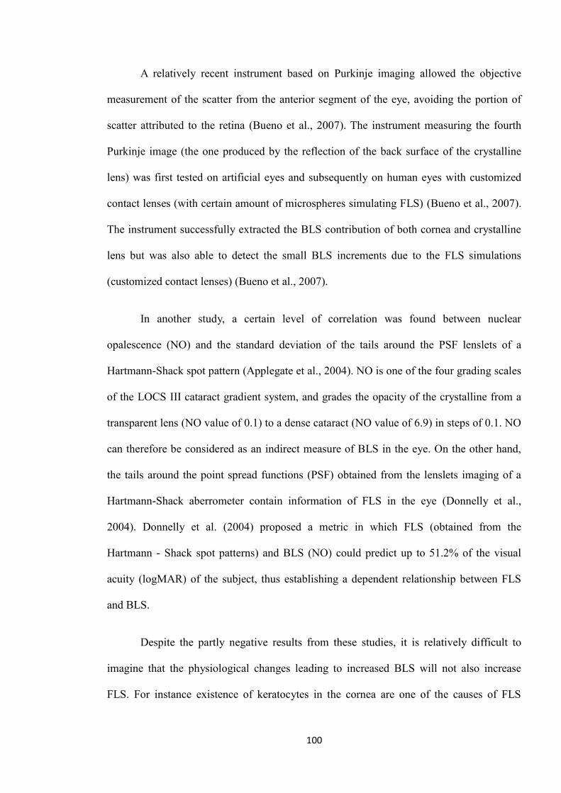
100

A relatively recent instrument based on Purkinje imaging allowed the objective

measurement of the scatter from the anterior segment of the eye, avoiding the portion of

scatter attributed to the retina (Bueno et al., 2007). The instrument measuring the fourth

Purkinje image (the one produced by the reflection of the back surface of the crystalline

lens) was first tested on artificial eyes and subsequently on human eyes with customized

contact lenses (with certain amount of microspheres simulating FLS) (Bueno et al., 2007).

The instrument successfully extracted the BLS contribution of both cornea and crystalline

lens but was also able to detect the small BLS increments due to the FLS simulations

(customized contact lenses) (Bueno et al., 2007).

In another study, a certain level of correlation was found between nuclear

opalescence (NO) and the standard deviation of the tails around the PSF lenslets of a

Hartmann-Shack spot pattern (Applegate et al., 2004). NO is one of the four grading scales

of the LOCS III cataract gradient system, and grades the opacity of the crystalline from a

transparent lens (NO value of 0.1) to a dense cataract (NO value of 6.9) in steps of 0.1. NO

can therefore be considered as an indirect measure of BLS in the eye. On the other hand,

the tails around the point spread functions (PSF) obtained from the lenslets imaging of a

Hartmann-Shack aberrometer contain information of FLS in the eye (Donnelly et al.,

2004). Donnelly et al. (2004) proposed a metric in which FLS (obtained from the

Hartmann - Shack spot patterns) and BLS (NO) could predict up to 51.2% of the visual

acuity (logMAR) of the subject, thus establishing a dependent relationship between FLS

and BLS.

Despite the partly negative results from these studies, it is relatively difficult to

imagine that the physiological changes leading to increased BLS will not also increase

FLS. For instance existence of keratocytes in the cornea are one of the causes of FLS

101

(Jester et al., 2007) and a study found that increased presence of keratocytes would also

increase corneal density measurement (Patel et al., 2001). For this reason, the present study

investigates whether BLS obtained as density measurements from the Oculus Pentacam

can be linked to the assessment of FLS from the C-Quant straylight meter.

4.6 METHODS

In order to evaluate the relationship between BLS and FLS, density analysis of the

cornea and the crystalline lens using Pentacam were assessed for a possible relationship

with C-Quant values. Therefore, the study evaluated the correlation between corneal

density (both peak and 3D), crystalline density (3D) and C-Quant straylight values.

Corneal thickness, although found previously unrelated to increased scatter (Olsen, 1982),

was included in the study and was also compared to C-Quant scatter values as different

corneal thicknesses were thought to affect the average density measurement obtained with

Pentacam (Olsen, 1982).

PARTICIPANTS

Twenty nine subjects were recruited from The University of Manchester student

and staff population. Ocular abnormalities (i.e. visible defects in eye structures), previous

ocular surgery and being a contact lens wearer (Nio et al., 2003) were considered as

exclusion criteria. The Pentacam PNS (Pentacam Nucleus Staging) tool was also used to

define the inclusion criteria. PNS was found useful to evaluate the density of nuclear

cataracts and its correlation to LOCS III up to a nuclear opalescence value equal to 5

(Magalhaes et al., 2011). In the present study, a PNS value equal to 0 was mandatory for all

the participants. PNS values equals to or greater than 1 considered the participant excluded

102

from the study as this value means a level of crystalline density unusually high for healthy

eyes, which might affect the analysis of the data. After applying that criterion, 26 subjects

were included in the analysis, with ages ranging from 19 to 35 years (29.92 ± 4.06

[mean±SD]) and spherical equivalent ranging from 0 to -8 (-1.9 ± 2.27 [mean±SD])

dioptres. Cylindrical power of the subjects ranged from 0 to -2 (-0.61 ± 0.57 [mean±SD])

dioptres. Although both eyes were tested, only right eyes were taken into consideration for

statistical analysis in order to minimize errors caused by the presence of strong correlation

between the two eyes (Ray and O'Day, 1985). The study followed the Declaration of

Helsinki Ethical Principles. Ethics approval was obtained from the University of

Manchester‟s ethics committee and written consent was obtained before participation in the

study. All measurements were made with natural pupil diameters under dim lighting

conditions.

MEASUREMENT WITH C-QUANT

Measurements with the C-Quant straylight meter are based on the compensation

comparison method (Franssen et al., 2006). This method consists of two half discs

surrounded by a flickering ring. The flickering ring is the glare source of achromatic light

and has an effective eccentricity angle of 7 degrees (van den Berg, 1995). The two halves

also flicker and the participant has to decide which half is flickering stronger. In this way,

when one of the halves flickers, flickering will also be perceived on the other half by

participants with certain levels of scatter in the eye. During the test, a two forced-choice

assessment and a psychometric function decides on the comparisons that will be presented

to the participant (Franssen et al., 2007). The results from this assessment are: the ocular

straylight value (log(s)) (van den Berg et al., 2013), the standard deviation (ESD) of

successively measured values and the quality factor of the psychometric function (Q)

103

(Coopens et al., 2006). An ESD value lower than 0.08 and Q value higher than 1 indicates

good reliability of measurements.

Measurements were obtained under scotopic light conditions. Participants‟ position

with respect to the instrument was checked (Van den Berg, 2014). Two valid measurements

(ESD<0.08 and Q>1) were obtained and averaged for each participant. Participants‟

refraction was corrected with their spherical equivalent refraction (Van den Berg, 2014)

when needed.

MEASUREMENT WITH PENTACAM

Pentacam (Figure 4.1) is an instrument based on Scheimpflug imaging that uses a

360⁰ camera with a blue LED light source (475nm) to obtain 25 Scheimpflug

monochromatic photographs (1003x520 pixels) of the eye. Each one of these photos

corresponds to a different meridian (ranging from 0 to 360⁰ with steps of 14.4⁰) of the eye.

Pixel intensities (densities) of these monochromatic photos are presented in grey scale

units and range from 0, for a maximum transparency and minimum light scatter detected

(black pixel), to 100 for maximum light scatter and minimum transparency (white pixel).

Measurements were considered as valid when the quality coefficient Q was equal to “OK”

and none of the 25 photographs presented any defects (part of the image missing or not

well aligned). Measurements took between 1 to 2 seconds and were obtained in scotopic

light conditions. Two valid measurements were obtained for each one of the participants.

The basic version of Pentacam was used in this study.

104

Figure 4.1: Scheimpflug image obtained with Pentacam. Peak corneal densitometry value

is the highest intensity pixel obtained from a histogram of the cornea for a certain

measured meridian (top right corner, in green). 3D corneal densitometry assessment

divides the cornea in concentrical zones around the pupil centre and provides with an

average density value for each zone. The optical axis is represented with the dotted red

line.

The Pentacam instrument comes with a basic densitometry software that can be

improved upon through premium add-ons (Table 4.1).

105

MEASURED

ZONE OF

THE EYE

BASIC PENTACAM

SOFTWARE

PREMIUM PENTACAM SOFTWARE

ADD-ONS

Cornea

Peak density (peak corneal

density value)

3D corneal density (average density value

measured at concentric zones from corneal

apex (0-2, 2-6, 6-10 and 10-12mm)

Corneal thickness

(measured at 0, 2, 4, 6, 8

and 10mm of eccentricity

from corneal apex)

X

Crystalline Peak density (peak

crystalline density value)

PNS (Pentacam Nucleus Staging) density

tool: Provides with a cataract grading scale

and a 3D crystalline density which gives an

average density level measured at

concentric zones from corneal apex

(PDZ1=0-2, PDZ2=0-4 and PDZ3=0-6mm)

Any part

Average linear density

(average density level

measured between 2 user

selected points on the

Pentacam density image)

X

Table 4.1: Types of density measurements and corneal thickness measurements available

in the basic version of Pentacam (software version 1.20r29).

Corneal density can be measured either using the Peak density analysis which is

integrated into the basic software package and gives a single peak density value for the

cornea at a measured meridian around the corneal apex (for a total of 25 meridians); or the

3D corneal density measurement (provided as a premium add-on) which gives an average

density value for a concentric volume around the corneal apex (0-2, 2-6, 6-10 and 10-

12mm of eccentricity) (Greenstein et al., 2010, Takacs et al., 2011, Otri et al., 2012) and

provides an average grey scale unit value for each one of them. The 3D corneal density

tool also subdivides the cornea into anterior layer (first 120µm of corneal thickness), centre

layer and posterior layer (last 60 µm of corneal thickness). Centre layer does not have a

fixed thickness as it depends on individual corneal characteristics and is the result of

deducting the sum of the anterior and posterior layers from the total corneal thickness of

the measured participant. Many studies have obtained measurements from subjects using

106

the peak corneal density analysis (Greenstein et al., 2010, Takacs et al., 2011, Otri et al.,

2012, Elflein et al., 2013). However, this method has been found to be less repeatable

compared to the 3D corneal density measurement (Kirkwood et al., 2009).

Crystalline lens density can be assessed by using the Peak density analysis which is

integrated into the basic Pentacam software and provides the highest density value for the

lens, for a meridian and around the corneal apex. Crystalline lens density can also be

measured using the PNS (Pentacam Nucleus Staging) premium add-on density tool. The

PNS tool provides a cataract grading scale similar to the one provided by the Lens

Opacification Classification System (Kirkwood et al., 2009, Magalhaes et al., 2011)

(LOCS III) (Chylack et al., 1993). The PNS tool also comes with a 3D crystalline density

measurement which provides an average density value measured at concentric volumes

around the corneal apex. These volumes are defined between: 0 and 2mm (PZ1); 0 and

4mm (PZ2); and 0 and 6mm (PZ3). In the Pentacam software, values for corneal thickness

are shown for 0, 2, 4, 6, 8 and 10mm of eccentricity.

Two valid measurements were obtained and averaged for each participant with both

C-Quant and Pentacam. In case of Pentacam, each valid measurement gives a total of 25

Scheimpflug images providing:

Peak densitometry: 1 value per image.

3D corneal densitometry: 1 value per each eccentricity (0-2mm, 2-6mm, 6-10mm,

10-12mm) and region (anterior, centre and posterior).

Corneal thickness: 1 value per eccentricity (0, 2, 4, 6, 8 and 10mm).

3D crystalline density: 1 value per each of the eccentricities (PDZ1 = 0-2mm,

PDZ2 = 0-4mm and PDZ3 = 0-6mm)

107


The distributions of the data from Pentacam and C-Quant were analysed for

normality with the Kolmogorov-Smirnov test (normality accepted for p value higher than

0.1 using the Lilliefors significance correction). The relationships between corneal

thickness, corneal density, crystalline density and C-Quant were assessed with two tailed

paired sample t-test and Pearson‟s correlation coefficient (r). A linear regression (least

squares) was performed to assess the contribution of BLS data from Pentacam density

measurements to FLS (C-Quant FLS values). A p-value of less than 0.05 was considered as

significant.



4.7 RESULTS

Normality was found for all the analysed data sets (p > 0.1). The participants‟ pupil

diameter measured with Pentacam (averaged from two valid measurements) ranged from

2.4 to 4.35mm (2.95 ± 0.52mm [mean±SD]). Values for the C-Quant straylight meter

(averaged from two valid measurements) ranged from log(s) = 0.73 to 1.27 (1.02 ± 0.06

[mean±SD]).

Peak corneal density: Average values ranged from 24.50 to 30.71 (28.15 ± 1.65

[mean±SD]). The correlation between these values and C-Quant values was not

statistically significant ( r = 0.31; p = 0.11).

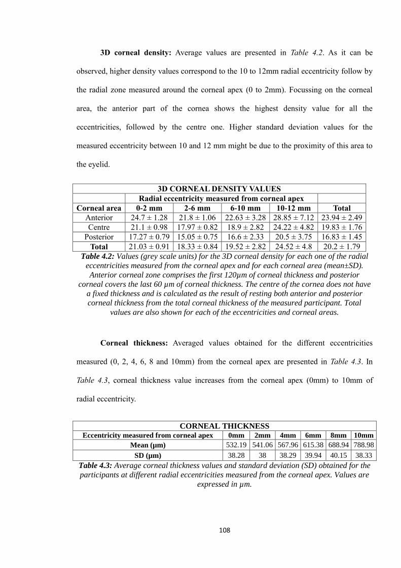
108

3D corneal density: Average values are presented in Table 4.2. As it can be

observed, higher density values correspond to the 10 to 12mm radial eccentricity follow by

the radial zone measured around the corneal apex (0 to 2mm). Focussing on the corneal

area, the anterior part of the cornea shows the highest density value for all the

eccentricities, followed by the centre one. Higher standard deviation values for the

measured eccentricity between 10 and 12 mm might be due to the proximity of this area to

the eyelid.

3D CORNEAL DENSITY VALUES

Radial eccentricity measured from corneal apex

Corneal area 0-2 mm 2-6 mm 6-10 mm 10-12 mm Total

Anterior 24.7 ± 1.28 21.8 ± 1.06 22.63 ± 3.28 28.85 ± 7.12 23.94 ± 2.49

Centre 21.1 ± 0.98 17.97 ± 0.82 18.9 ± 2.82 24.22 ± 4.82 19.83 ± 1.76

Posterior 17.27 ± 0.79 15.05 ± 0.75 16.6 ± 2.33 20.5 ± 3.75 16.83 ± 1.45

Total 21.03 ± 0.91 18.33 ± 0.84 19.52 ± 2.82 24.52 ± 4.8 20.2 ± 1.79

Table 4.2: Values (grey scale units) for the 3D corneal density for each one of the radial

eccentricities measured from the corneal apex and for each corneal area (mean±SD).

Anterior corneal zone comprises the first 120µm of corneal thickness and posterior

corneal covers the last 60 µm of corneal thickness. The centre of the cornea does not have

a fixed thickness and is calculated as the result of resting both anterior and posterior

corneal thickness from the total corneal thickness of the measured participant. Total

values are also shown for each of the eccentricities and corneal areas.

Corneal thickness: Averaged values obtained for the different eccentricities

measured (0, 2, 4, 6, 8 and 10mm) from the corneal apex are presented in Table 4.3. In

Table 4.3, corneal thickness value increases from the corneal apex (0mm) to 10mm of

radial eccentricity.

CORNEAL THICKNESS Eccentricity measured from corneal apex 0mm 2mm 4mm 6mm 8mm 10mm

Mean (µm) 532.19 541.06 567.96 615.38 688.94 788.98

SD (µm) 38.28 38 38.29 39.94 40.15 38.33

Table 4.3: Average corneal thickness values and standard deviation (SD) obtained for the

participants at different radial eccentricities measured from the corneal apex. Values are

expressed in µm.

109

The correlation found between corneal thickness and C-Quant FLS values for each

of the eccentricities measured was: 0mm (r = 0.06, p = 0.76), 2mm (r = 0.06, p = 0.77),

4mm (r = 0.06, p = 0.77), 6mm (r = 0.07, p = 0.73), 8mm (r = 0.07, p = 0.75) and 10mm (r

= 0.03, p = 0.89).

3D crystalline density: Pentacam was not able to capture the density value of the

crystalline lens for the larger measured eccentricity (PDZ3=0-6mm) in most participants

and hence it was not taken into consideration. PDZ1 values ranged from 8 to 11.35 (9.61 ±

0.77 [mean±SD]) while PDZ2 values ranged from 8.5 to 11.45 (9.75 ± 0.72 [mean±SD]).

Graph 1 shows the BLS (average 3D corneal density values (Total 0-2 mm) and the

average 3D crystalline density (PDZ1)) as a function of C-Quant straylight meter values

(FLS). In both cases, a weak and statistically insignificant relationship was found: average

3D corneal density values (Total 0-2 mm) and C-Quant (y = 2.16x + 18.84, r2 = 0.1, p =

0.11); average 3D crystalline density (PDZ1) and C-Quant (y = 0.68x + 8.92, r2 = 0.01, p =

0.56).

110

Figure 4.2: Average 3D corneal density values (Total 0-2mm) and the average 3D

crystalline density (PDZ1) in grey scale units as a function of C-Quant (log(s)).

4.8 DISCUSSION

The study assessed whether a relationship that could be found between density

maps due to BLS (obtained with Pentacam) and FLS as measured with the C-Quant. The

study is based on a young healthy population with very low levels of crystalline lens

y = 2.1561x + 18.835

r² = 0.10

p = 0.11

y = 0.6843x + 8.916

r² = 0.01

p = 0.56

7,5

9,5

11,5

13,5

15,5

17,5

19,5

21,5

23,5

0,6 0,8 1 1,2 1,4

Aver

age

3D

corn

eal

den

sity

(tota

l 0

-2m

m)

in g

rey s

cale

un

its

C-Quant straylight meter values (log(s))

Aver

age

3D

cry

stall

ine

den

sity

111

density (PNS levels equal to 0 were considered as inclusion criteria) and non-dilated

pupils.

In this study, BLS measurements with Pentacam were performed using the peak

density and 3D density analysis in case of the cornea. Crystalline density was assessed

using the 3D density analysis. Another study suggested that repeatability improves with the

averaging of 3D density values and decreases when using single peak values (Kirkwood et

al., 2009). Furthermore, high repeatability and validity of the 3D density analysis of ocular

lenses was found in subjects with and without cataracts (Kirkwood et al., 2009).

Corneal density results obtained for this study differ depending on the type of

measurements used: peak or 3D analysis. For the peak density analysis, 28.15 ± 1.65

(mean ± SD) grey-scale units while 20.20 ± 1.79 (mean ± SD) for the 3D one. These

results are in agreement with a previously published study (Ni Dhubhghaill et al., 2014)

and make sense considering the way of measurement: the value obtained by the peak

density analysis is the result of a single peak value measured for the corneal lens along one

meridian, while the 3D measurement provides an average value of a cylindrical volume of

the cornea around the corneal apex, which covers 0-2, 2-6, 6-10 and 10-12 mm of

eccentricity.

Peak corneal density measurements have been found to be related to the LOCS III

cataract grading system (Pei et al., 2008). However, the limitations of this measurement

(peak value for a single line along the cornea and for certain meridian) compared to the 3D

corneal density measurement showed also less repeatability (Kirkwood et al., 2009).

Results obtained from the 3D corneal density analysis indicate that higher density

levels for the anterior corneal layer in every measured eccentricity coincide also with a

higher density of keratocytes for that layer (Patel et al., 2001) and therefore with an

112

increased level of intraocular scatter (Jester et al., 1999). However, if the relationship

between BLS and FLS existed, measurements from the 3D corneal density would be

expected to correlate better with FLS values (Figure 4.2) as crystalline lens density values

were intended to be as low as possible for the study (PNS = 0). This fact should also have

conditioned the C-Quant values, making the scatter contribution from the cornea a larger

part of it.

In one study (Wu et al., 2014) results obtained from the 3D corneal density analysis

and compared to C-Quant values showed a slightly better yet negative agreement for the

eccentricities of 0-2 (r = 0.13, p = 0.04), 2-6 (r = 0.15, p = 0.03) and 6-10mm (r = 0.16, p =

0.02) (Wu et al., 2014). These results (Wu et al., 2014), which have also different 3D

corneal density values from the ones obtained in this study (and a larger previous study

with similar results to the present study (Ni Dhubhghaill et al., 2014)), might be due to

differences in the software used for the density measurement of the Pentacam images, units

conversion or saturation of the processed density images.

Corneal thickness measurements obtained in this study are in agreement with a

previous study in which the repeatability of the corneal thickness measurements was

positively assessed using Pentacam (Miranda et al., 2009). Corneal thickness was

previously found not to affect FLS measurements (Wu et al., 2014).

In this study, the peak crystalline lens density was measured, but not taken into

account for calculations as it was found to be dependent on the amount of light reaching

the crystalline lens for each one of the meridians. The selection of participants with low

levels of crystalline density (PNS = 0) for this study might be the reason for the change of

shape of the crystalline density map obtained for each one of the meridians. In addition,

due to this study assessing a small radial zone of cornea and crystalline around the corneal

113

apex, pupils were not dilated. This fact might have limited the validity of the 3D crystalline

density measurements (even when the quality factor Q equals to “OK” and none of the 25

photographs presenting any defects) of the crystalline lens with non-dilated pupils to

values PDZ1 = 0-2mm and PDZ2 = 0-4mm (excluding PDZ3 = 0-6mm) of eccentricity.

Furthermore, one study showed that measurements of the posterior capsule of the

crystalline lens can be difficult even if the pupil is totally dilated (Fujisawa and Sasaki,

1995). To our knowledge, no studies are available in the literature evaluating whether

Pentacam density values in dilated and non-dilated pupils differ. In this sense, a study has

suggested this comparison to ensure that Pentacam can be used for mass screening (Lim et

al., 2014). This lack of illumination is not only appreciable at the back of the crystalline

lens, but also when measuring near the eyelids or eyelashes. This effect produces a great

variability on the 3D corneal density measurements as seen with the increase of the

standard deviation, especially for the 10-12mm eccentricity (Table 4.2).

Density values (grey scale units) obtained for the 3D crystalline density

measurements are almost half the value of the 3D corneal density values. This comparison

contradicts the purpose of this study which is to compare BLS and FLS, since scatter

contribution of the crystalline lens to the total FLS is supposed to be higher than that of the

cornea (Vos and Boogaard, 1963). The weak agreement observed between 3D crystalline

density values and C-Quant values (Figure 4.2) might be due to the lack of pupil dilation.

The study has considered the two most important ocular FLS sources which are the

cornea (30%) (Vos and Boogaard, 1963) and the crystalline lens (40%) (Bettelheim and

Ali, 1985) (cornea and crystalline). BLS from cornea and crystalline lens should have

accounted with similar amounts in case of agreement. This lack of agreement may,

however, be explained by various factors. Firstly, the BLS value obtained by Pentacam

114

might be a measure of light reflection (Rosales and Marcos, 2009). Our hypothesis that the

structure causing this reflection/BLS would also produce significant FLS may be incorrect.

FLS is mainly a combination of Mie/geometric scatter rather than Rayleigh scatter while

BLS is the opposite (Born and Wolf, 1980, van den Berg, 1997, van den Berg and

Spekreijse, 1999). In this sense, multillamellar bodies, which are the main FLS source in

the crystalline lens, can be explained by the Mie theory (van den Berg, 1997, van den Berg

and Spekreijse, 1999, Vos, 2003, Costello et al., 2007). Secondly, density values of both

cornea and crystalline lens have not been considered with respect to their thicknesses. The

thickness of the ocular scatter particles defines their scatter behaviour (FLS or BLS) (van

den Berg, 1997, van den Berg and Spekreijse, 1999). This analysis of the scatter particles

using Pentacam BLS images would allow the corneal and lens correction algorithms of

Dubbelman et al. (Dubbelman and Van der Heijde, 2001, Dubbelman et al., 2001,

Dubbelman et al., 2006) and might give a better approximation to FLS using BLS images.

Unfortunately, Pentacam raw images can only be analysed by using the software provided

by the manufacturer (Rosales and Marcos, 2009) and the tools available with such

software. Extraction of raw images for extra analysis are also limited due to proprietary

limitations and only custom made programs can give access to such images (Rosales and

Marcos, 2009).

115

5. INSTRUMENT AND COMPUTERIZED

BASED MODEL FOR THE OBJECTIVE

MEASUREMENT OF FORWARD LIGHT

SCATTER

5.1 CONTRIBUTIONS

The study was designed by my co-author (Vincent Nourrit) and me. The optical set-up was

initially suggested by J. Barbur (City University, London). The data collection and the

analysis of the study were done by me with useful advice from my co-author. The writing

of the study was done by me and my co-author.


Target journal: Journal of Biomedical Optics. Authors: Pablo Benito Lopez and Vincent

Nourrit. To be submitted.


This paper has been submitted to the Visual and Physiological Optics meeting, held in

Wroclaw (Poland) from the 25th

to the 27th

of August 2014 (EMVPO) before being

116

withdrawn. However, the EMVPO organizing committee still published it in the

proceedings (Benito Lopez et al., 2014).

5.4 ABSTRACT

BACKGROUND: In the last decade, several instruments have been introduced to measure

objectively and accurately intraocular forward light scatter (FLS). Unfortunately, these

measurements cannot be related precisely to any physiological factors.

PURPOSE: To develop an instrument together with a model with a view to obtain

accurate FLS measurements that can be related to the sources of scatter.

METHODS: An optical set-up was developed where a subject or an artificial eye looks at

an LED ring, placed at a fixed distance, and the retinal image of the ring is recorded with a

CCD camera (double pass configuration). Firstly, the validation of the instrument was

conducted by an artificial eye, where the scatter was produced by a microscopy plate

containing a layer of silica microspheres. A non-sequential Zemax model of this set-up was

also developed in order to relate the experimental measurements to the parameters of the

optical system. In both – the optical set-up and Zemax model – the amount of forward light

scatter was assessed from the distribution of light inside the ring of imaged LEDs on the

CCD. Secondly, ten participants were tested with the optical set-up. The scatter

measurements in human eyes were compared with the FLS values obtained from the C-

Quant straylight meter. A Zemax model of the human eye, including scatter structures, was

also developed and compared to the measurements obtained on participants with the

optical set-up.

117

RESULTS: The amount of light scattered in the artificial eye was successfully recorded

by the instrument and was in good agreement with the Zemax model of the optical set-up.

Human eye measurements also related well with C-Quant straylight meter values. Scatter

from the Zemax eye model could not be positively related to the human eye measurements.

CONCLUSIONS: Results with the artificial eye suggested that the proposed optical set-

up can provide the means to assess FLS objectively and that the FLS measurement can be

related to a physical parameter through the Zemax model (e.g. scatter particle density).

Results in human eyes correlated well with measurements obtained with the C-Quant (r² =

0.75; p < 0.05) but cannot yet be explained by the developed Zemax model.

5.5 INTRODUCTION

Our vision is often described as limited by three optical factors: aberrations,

diffraction and light scatter. While diffraction is inherent to any optical system and

aberrations can be successfully corrected through various means (e.g. spectacles,

surgery), scatter increases with age and irremediably reduces our visual performances.

The importance of the FLS lies in its effect on the quality of the retinal image because of

the reduction of contrast sensitivity and the increase in disability glare (De Waard et al.,

1992). As a result, the amount of FLS could be for instance the deciding factor in cataract

surgery (Bal et al., 2011) or limiting in visually demanding jobs (Van Bree et al., 2011).

Despite the importance of FLS there is currently no instrument to measure it

objectively and to relate it to physiological parameters. The purpose of this study is to

address this lack. In section 5.6 the literature related to the measurement and modelling

118

of FLS is reviewed before the methods used for this study are presented (5.7). Results and

discussion are shown in sections 5.8 and 5.9 respectively.

5.6 REVIEW OF FLS MEASURING AND MODELING

5.6.1 MODELLING FLS

5.6.1.1 Modelling the physiological sources of scatter

In contrast to low order aberrations that can be related to few simple

physiological parameters, the origin of FLS is complex. FLS in the healthy human eye

corresponds to 1-2% of the incoming light (Vos, 1984). For a healthy eye, up to 30% of the

FLS comes from the contribution of the cornea (Vos and Boogaard, 1963), 40% from the

crystalline (Bettelheim and Ali, 1985), 10% from the vitreous (Koenz et al., 1995) and

another 20% is due to the retina (Vos and Bouman, 1964). A small fraction of the FLS

(≤1%) can also be attributed to transillumination through the iris (van den Berg et al.,

1991).

Regarding the cornea, the anterior surface of the epithelial cell layer and the

posterior surface of the endothelium were found to be the major sources of scatter when

using in-vivo confocal microscopy (Jester, 2008). Scatter from the stroma is limited to

Keratocytes nuclei (Jester, 2008) as demonstrated by the good relationship between

decrease in the density of keratocytes and the reduction of FLS (Jester et al., 2007). These

keratocytes occupy a volume of 9-17% within the stroma and have a density of 23000

cells/mm3 in human eyes (Hahnel et al., 2000, McLaren et al., 2005). Keratocytes nuclei

119

have a thickness of 1µm (Hahnel et al., 2000) and an average refractive index of 1.401

(Patel et al., 2001).

Regarding the crystalline lens, scatter is due to the aggregation of protein

molecules in the crystalline’s nucleus (Bettelheim and Ali, 1985) and mainly because of

the posterior migration of cells from the epithelia creating large organelles called

multillamellar bodies (Gilliland et al., 2001, Gilliland et al., 2004). Multillamellar bodies

have a density of 556 cells/mm3 for healthy crystalline lenses, a diameter of 2.7±0.7µm

and an average refractive index of 1.49 (Gilliland et al., 2004, Costello et al., 2007).

5.6.1.2 Modelling light propagation within the eye

The absence of an instrument to relate the FLS measurements to a physiological

parameter is probably due to the structural complexity of the human eye, but also the

associated difficulty to describe light propagation within the eye.

Over the last 150 years, numerous eye models have been proposed with

increasing complexity (aspheric surfaces, GRIN, etc. (see (Navarro, 2009) for a review).

Some of the models allow taking into account scatter elements (e.g. (Kelly-Pérez et al.,

2011, Chen et al., 2012, Kelly-Perez et al., 2013) when the scatter sources are arbitrarily

defined (e.g. number and distribution of scatter particles in the crystalline lens (Kelly-

Perez et al., 2013).

Due to the geometric dimensions of the eye and the limited influence of

diffraction, propagation through such models has usually been carried out using

120

geometrical optics. When field propagation is considered, calculations are usually limited

to the measurement of the Fourier transform of the wavefront in the pupil´s plane. Mas

et al. proposed an interesting model to simulate wave propagation inside the eye and

along any distance using Fractional Fourier transform (Mas et al., 2009). Although

theoretically superior to the geometrical models, the main limitations of these

approaches are: the discrepancy between the complexity of the calculations and the lack

of accuracy to characterize the different ocular elements. For instance, the characteristics

of the crystalline lens: tilt, decentring, GRIN, etc. are known with limited accuracy and

thus discourage researchers from pursuing a sophisticated model.

5.6.2 MEASURING FLS

Methods to assess FLS are usually divided into two groups depending on whether

they require or not active participation from the tested participants.

Methods that automatically (without the subject´s input) assess FLS rely on the

analysis of a retinal image while a glare source is being presented to the eye (usually the

assessment of the point spread function (PSF) through double pass techniques

(Santamaría et al., 1987, Artal et al., 1995, Kuroda et al., 2002, Donnelly Iii et al., 2004)).

The main issue with this approach is the difficulty to measure small angle scatter due to

the large dynamic range of the signal and the fact that the centre of the PSF is mainly

controlled by aberrations. In this context, a recent study from Ginis et al. presents a

promising instrument that can reconstruct the wide-angle PSF up to 8 degrees (Ginis et

al., 2012).

121

The methods based on subjects´ response assess the contrast sensitivity in the

presence of a glare source. The two most successful methods are probably the direct

compensation technique (van den Berg, 1986) and the compensation comparison method

(Franssen et al., 2006). The latter is based on the direct compensation technique but with

a psychophysical analysis that improves the repeatability substantially. On the contrary to

the methods not relying on the subject´s input, these methods assess the domain of the

PSF corresponding to large angle scatter (Van Den Berg et al., 2009) as depicted in Figure

5.1.

Figure 5.1:PSF plot the human eye and domains covered by the different FLS measuring

techniques (Van Den Berg et al., 2009).

The information obtained by the current instruments to measure FLS does not

always correlate well with physiological factors (cf. previous chapters of this PhD thesis).

122

The aim of this study was therefore to develop an instrument together with a model to

obtain accurate and reliable FLS measurements and to account for the source of scatter.

5.7 METHODS

The study was divided into two parts. Firstly, an optical bench was set up where a

subject or an artificial eye, looks at a LED ring placed at a fixed distance, and the retinal

image of the ring is recorded by a CCD camera (in a double pass configuration). The

artificial eye was made of a mirror and a lens. Determined levels of light scatter were

produced with a microscopy plate and a layer of silica microspheres whose properties are

known (index of refraction, diameter, and density). Four microscope plates containing

increasing density levels of silica microspheres were used to simulate increased levels of

scatter. A non-sequential Zemax model of this set-up was also developed. Mie scatter was

introduced in the Zemax model to simulate the scatter produced by the silica microspheres.

In both – the optical set-up and the Zemax model – the light distribution within the retinal

image of the ring was analysed. Details of the optical set-up are introduced in sub-section

5.7.1.

Once the agreement between experimental set-up and model was validated, scatter

measurement from human eyes was obtained with the prototype and compared with scatter

values from the C-Quant straylight meter. The eye model and recruitment criteria for

patients are described in section 5.7.2.

123

5.7.1 EXPERIMENTAL SET-UP USED FOR EXPERIMENT 1 AND 2

The optical double pass instrument is depicted in Figure 5.2.

Figure 5.2: Optical set-up for the objective measurement of FLS. Light from the light

source (LEDs ring) is reflected by the beam splitter into the eye. This light is then reflected

by the retina and transmitted by the beam splitter into a series of lenses (L1, L2 and L3)

and apertures (D1 and D2) and finally recorded into a CCD camera. CCD, retina and

light source are conjugated. D1 eliminates diffuse reflection from the cornea while letting

FLS pass through. D2 blocks specular reflexions from the cornea.

In summary, the eye looked at the light source (LEDs ring) through the beam

splitter (BS) (Thorlabs BP108 - Ø1" pellicle beam splitter, uncoated for a

reflexion:transmission ratio of 8:92). The light from the LED ring was then reflected by the

retina and captured by the CCD camera after passing again through the pellicle beam

splitter (BS) and a series of lenses (L1-L2-L3) and apertures (D1-D2). The CCD, the retina

and the light source (LEDs ring) were conjugated. The source of light (the chromaticity

coordinates are X:0.287-0.330, Y:0.295-0.318) was composed of 16 white LEDs (Nischia

LED 5mm white 44000mcd NSPW500GS-K1) of 5mm width each, forming a circle of 1.78

centimetres of radius. The LEDs ring could be moved mechanically to vary the distance

124

light source - eye. The smallest angle of observation had to be greater than 7 minutes of

arc in order to be outside the PSF (Westheimer and Liang, 1995). With this LED circle,

different eccentricities with respect to the optical axis (eye - LED ring) could be measured

for each distance of the LED ring with respect to the eye. D1 was conjugated with the

retina and thus stopped unwanted signals such as diffuse reflection on the cornea and

retina. On the contrary, D2 allowed passing only light coming with an angular eccentricity

larger than the centred black circle. D2 was made of an uncoated transparent plastic film

with a black dot at the centre and its aim was to block the incoming light caused by

specular reflection from the cornea.

The amount of light captured with the CCD in the centre of the annulus was

proportional to the level of scatter inside the eye. In the absence of scatter, all the light

originated in the LEDs should be concentrated in their respective image. The image of the

LEDs ring on the retina was recorded using a CCD camera (Rolera XR, Qimaging, BC,

Canada) and processed with the program Q-Capture version 2.901 (Qimaging, BC,

Canada), obtaining an image size of 696x520 pixels and a pixel size of 12.9 x 12.9µm. The

optical path of the set-up was protected with a black flocking material in order to avoid

unwanted reflections or the apparition of artefacts.

MEASUREMENT OF FLS

Noise from the system, meinly due to back reflections from the pellicle beam

splitter, was measured at the beginning of each measuring session in scotopic conditions.

The pixel intensity produced by the noise was measured and later deducted from the

recorded CCD image. The intensity profile across a diameter of the LED ring is presented

in Figure 5.3 where the blue line represents the signal recorded by the instrument and

125

the red line corresponds to the noise signal. The two peaks correspond to the LEDs profile

image. The fact that the instrument signal between the two peaks is not reduced by the

noise level illustrated the presence of scatter.

Figure 5.3: Pixel intensity profile recorded by the CCD. Red line

corresponds to the instrument noise. Blue line shows the recorded LEDs

pixel intensity (peaks) and the amount of scatter (intensity recorded within

the two peaks). Intensity per pixel measured in this simulation at the centre

of the two peaks is about 5 times higher than the level of measured noise.

The pixel intensity produced in case of aberrations due to subjects´ eye

should have given a homogenous scatter pattern for all the CCD image

(and not only in the centre of the ring, also outside) and with a similar

intensity signal to the one produced by the noise in that graph.

The CCD exposure time was chosen (empirically) to maximize the intensity

detection at the centre of the LEDs ring at the camera sensor.

126

A customized software was developed in Matlab to analyse the images obtained

from the CCD camera. The software took the images recorded from the CCD (centre of

the LED ring reflected from the retina) and corrected them from the noise signal

(deducted an image obtained prior to measurements with artificial/human eye).

Subsequently, the average intensity per pixel in the central area of the LED ring was

calculated.

5.7.2 FIRST EXPERIMENT: VALIDATION OF THE PROTOTYPE

WITH CUSTOMISED LENSES AND ZEMAX MODEL

An artificial eye was used for this part of the experiment. The eye consisted of a

lens of 62.5D (F=16mm, diameter=1”) and a mirror. This specific lens was selected for the

experiment as the size and the dioptric power were similar to the ones presented in a

human eye. The mirror was used instead of retina in order to reduce the modelling

complexities.

The source of scatter was created with an uncoated microscope plate which was

covered with a layer of a polymer solution and a microscope plate cover on top. The

polymer solution contained a determined percentage of silica microspheres whose

properties are known (Monodisperse Silica Microspheres, mean diameter 4.08um, index of

refraction = 1.45, Cospheric, U.S.A.). The diameter of microspheres was chosen in order to

simulate the diameter of the scatter sources that can be normally found within the human

eye (i.e. keratocytes). Four microscope plates with increasing levels of microspheres

density were used to simulate increased levels of scatter. These microscope plates where

placed between the lens and the mirror. A distance of 50 cm between the light source and

127

the artificial eye was considered. All images were taken in scotopic light conditions. The

„noise‟ image was recorded before each measurement.

In summary, three series of pictures were recorded for each of the following scatter

sources (i.e. a total of 12 images):

Microscopy slide alone (index of refraction n=1.51) + polymer (n=1.30) + cover

(n=1.51).

Microscopy slide (n=1.51) + 1% concentration of microspheres (n=1.45) + polymer

+ cover.

Microscopy slide + 2% concentration of microspheres + polymer + cover.

Microscopy slide + 3% concentration of microspheres + polymer + cover.

The modelization of the prototype was made by using the optical design software

Zemax_EE 2009 (Radiant Zemax, Redmond, U.S.A.) in non-sequential mode, together

with a scatter library, Mie.dll (provided by Zemax software) to simulate MIE scatter.

Values of density (percentage concentration of microspheres per volume), index of

refraction and average microsphere diameter (4.08 µm) were added to the design for each

one of the microscope plates. For comparison between simulations (Zemax) and

experimental results (microscopy plates in the artificial eye), the following ratio was

calculated for each one of the microscopy slides:

I i y igh wi hi h h LED i g’ i g i h i h

I i y igh wi hi h h LED i g’ i g i h b i h

The intensity of scatter light recorded in the absence of scatter microspheres

(microscopy slide alone) by the CCD corresponded to a number of analysis rays defined by

128

the user in Zemax. In this study, 5x106 analysis rays were sent into the Zemax model of the

artificial eye for the simulation.

5.7.3 SECOND EXPERIMENT: RESULTS FROM PARTICIPANTS,

COMPARISON RESULTS PROTOTYPE / C-QUANT AND

PROTOTYPE / ZEMAX SCATTER EYE MODEL

In order to maximize the alignment eye - optical system during measurements with

participants, a chin rest was added to the set-up. Moreover, an additional aperture was

placed in front of the chin rest with the adequate diameter to facilitate the task of alignment

by the subject to the optical system.

The pupillary diameter (assessed with a pupillary ruler), distances from the light

source to participants´ pupil and light intensity level of the light source were measured for

each one of the participants (Bergamin and Kardon, 2003).

The measuring technique was the following:

A first image in the absence of human eye is taken to calculate the noise of the

instrument.

After placing the chin of the subject on the chin rest and adjusting the distance eye

– light source and the intensity level of the light source, the subject was asked to

look at the centre of the ring. Two valid measurements (images without artefacts

and well-aligned images) were obtained and averaged for a determined distance

and intensity level of the light source. Subsequently, average intensity per pixel

129

recorded by the CCD camera was calculated for the ten participants and compared

to FLS values from C-Quant.

All measurements were done under scotopic light conditions. The distance eye – light

source was set to 50 cm. Participants were asked to focus on the centre of the LEDs ring.

MEASUREMENT WITH C-QUANT

The C-Quant straylight meter (Figure 5.4) uses the compensation comparison

method (Franssen et al., 2006) for the assessment of FLS. Essentially, a test field is

presented to the subject consisting of two half discs surrounded by a ring. This ring is the

glare source of achromatic light and has an effective eccentricity of 7 degrees (van den

Berg, 1995). During the assessment, a series of 2-forced choice tests are presented to the

subject. The subject has to decide, while the glare source flickers, which one of the two

inner half discs is flickering the most. FLS will be perceived by the subject as a flickering

on the non-flickering half disc. A psychometric function (Franssen et al., 2007a) adapts the

type of test presented to the subject and the results for this assessment are three values: the

straylight parameter (log(s)), the standard deviation of the measurement (ESD) and a

quality factor (Q) (Coopens et al., 2006).

130

Figure 5.4: C-Quant stimulus screen. The instrument has a glare source with angle of 5 to

10 degrees with respect to the eye (7 degrees of effective scatter angle). The flickering


field is composed of a circle with two half discs.

The assessment with C-Quant is performed under scotopic light conditions after

checking that the subject‟s position with respect to the instrument is correct. Participants

with any refracted error were corrected with their spherical equivalent correction (Van den

Berg). A valid measurement of FLS (log(s)) is considered when the standard deviation of

the measurement is lower than 0.08 and quality factor higher than 1. Two valid

measurements were obtained for each one of the participants and averaged.

For this study, ten participants underwent the experiment. Visible defects in the eye

structures (with slit-lamp examination), history of ocular diseases or previous ocular

surgery were considered as exclusion criteria. Due to the lack of a mechanism to control

the pupillary miosis of the eye in bright conditions (LEDs), only participants with pupillary

diameters (in miosis) larger than the measured eccentricity (2.04º) were considered. Age of

the participants ranged from 29 to 35 (32 ± 2.16 [mean±SD]) years. Spherical equivalent

ranged from -3.25 to 1.25 (-0.8±1.57 [mean±SD]) dioptres. Only right eyes were tested and

taken into consideration for statistical analysis.

131

ZEMAX EYE MODEL OF SCATTER AND MEASUREMENT

The model of scattering in the human eye was done in Zemax non-sequential mode

and using the MIE scatter tool to simulate bulk scatter within the lenses.

The model was based on the physiological parameters of the eye obtained by Liou

& Brennan (Liou and Brennan, 1997). This model was chosen because it offers a good

compromise between simplicity and anatomic realism. For instance, it allows taking into

account factors such as aspheric surfaces for the cornea and lens, a curved surface for the

retina, or a gradient refractive index for the crystalline lens. Major characteristics of this

model are shown in Table 5.1.

Ocular Surface Radius (mm)

Thickness (mm)

Asphericity Refractive index

(555nm)

Cornea 7.77 0.50 -0.18 1.376

Aqueous 6.40 3.16 -0.60 1.336

Front crystalline

12.40 1.59 -0.94 Gradient A

Back crystalline Infinity 2.43 ------- Gradient B

Vitreous -8.10 16.27 0.96 1.336

Gradient A = 1.368+0.049057 * z - 0.015427 * z2 – 0.001978 * r2 Gradient B = 1.407 – 0.006605 * z2 – 0.001978 * r2

n(λ) = n(0.555µm) + 0.0512 – 0.1455 * λ + 0.0961 * λ2

Table 5.1: Main characteristics of Liou-Brennan model eye for each of the ocular

surfaces.

The same Zemax model of the optical set-up from the previous section was used for

this part of the experiment. However, the artificial eye was changed by the human eye

model. Intraocular scatter within the eye model was due to the bulk scatter added at the

level of the cornea and crystalline lenses. Keratocytes and multillamellar bodies were

added as scatter sources for the cornea and crystalline lens respectively. The data for the

simulation of these scatter sources (density, index of refraction and size) is presented in

section 5.6.1.1.

132

Two different measurements of the scatter were obtained from this eye: the total

scattered light captured by the CCD and the average intensity per pixel recorded in the

central area of the CCD ring image. In order to measure the total light scatter captured by

the CCD, a transparent filter was introduced to the current Zemax model optical set-up.

The filter was placed between D2 and L3 (Figure 5.2) and its function was to block any

rays coming from the eye that are not perpendicular to its surface. According to the design

of the optical set-up, rays from the light source passing through an eye without scatter will

be perpendicular to D2 and L3 in their trajectory to the CCD. In the presence of intraocular

scatter within the model eye, rays not perpendicular to D2 and L3 will be due to scatter and

will not pass this filter. A percentage of FLS within the model eye was obtained by

recording the amount of rays captured by the CCD camera and the ones blocked by the

filter. Both measurements were the result of averaging 5 simulations.


The Kolmogorov-Smirnov test was used to assess the normality of the data.

Relationships between variables were assessed with two tailed paired sample t-test and

Pearson‟s correlation coefficient. A p-value inferior to 0.05 was considered as significant.



133

5.8 RESULTS



In order to compare the results obtained from the CCD sensor of the prototype and

the ones obtained from the Zemax model, the dimensions of the images of the light source

(LEDs ring) were checked. The image of both rings (CCD sensor and Zemax) had a

diameter of 1.3 mm (measured from the centre of the LEDs). Noise obtained from the

optical system compared to scatter signal had a ratio of about 1:5.

Figure 5.5 shows an image recorded by the CCD obtained as a result of the

measurement of a microscopy plate with certain level of scatter. The diameter of the central

area used for calculation (inside blue circle) was fixed to 1mm. This size allowed

measuring just the contribution of light scatter obtained in the centre of the LED ring and

not intensity from the LEDs. This area (one millimetre of diameter) corresponded also to

the area inside the LEDs circle (on both CCD image of the optical set-up and Zemax

model) where no pixel intensity is detected in absence of a scatter source (artificial eye

with microspheres or a human eye) and when the noise is removed.

Figure 5.5: Recorded image from the optical prototype. The central area used for

calculations (inside blue circle) has a diameter of 1mm. Brightness changes of LEDs

correspond to the particular radiation patterns (narrow viewing angle) of the LEDs and

the difficulty of alignment.

134

Figure 5.6 represents the results obtained in Zemax for each one of the microscopy

slides tested. As scatter increases, the intensity per pixel distribution of light spread on the

central measuring area rises, making the peaks corresponding to the cross section profile

decrease in height.

Figure 5.6: Light distribution obtained in Zemax for each one of the microscopy slides

tested. A) Microscopy slide alone. B) Microscopy slide + solution of polymer with 1% of

concentration of microspheres. C) Microscopy slide + 2% of microspheres concentration.

D) Microscopy slide + 3% of microspheres concentration. Cross sectional profiles are

also shown above.

Figure 5.7 depicts a comparison of the different intensity profiles obtained for each

of the microscopy slides with different concentration of microspheres (microscopy slide

alone, 1, 2 and 3% density of microspheres) using Zemax. Only the central area between

the two peaks is measured for the calculation of light scatter.

135

Figure 5.7: Comparison of the cross sectional profiles obtained for the 4 microscopy

slides tested using Zemax. Red line correspond to the microscopy slide alone, orange =

1% density of microspheres, blue = 2% and green = 3%. The intensity of the central part

between the two peaks (measuring area) increases in accordance to light scatter. Profiles

have been smoothed to make the visual comparison easier. In the absence of scatter

sources, the recorded intensity is null in the central zone (1mm of diameter).

Table 5.2 represents the average intensity per pixel obtained from the central part of

the CCD image after being processed with Matlab for each one of the microscopy slides.

Microscopy plate Average intensity pixel

value (optical set-up)

Zemax measurements

(intensity ratios)

1 27.9 ± 2.36 1

2 59.27 ± 2.66 1.88 ± 0.032

3 100.74 ± 3.25 3.72 ± 0.026

4 140.32 ± 4.56 5.44 ± 0.03

Table 5.2: Scatter values obtained from the measuring areas for the optical set-up and

ratios from Zemax for the different microscopy plates.

Figure 5.8 depicts the results of the comparison between scatter obtained through

the optical prototype and its Zemax model. A good relationship was found between

measurements (r² = 0.98; p < 0.05). In Figure 5.8, the amount of “scatter” due to the

136

microscopic plate alone is due to multiple reflections within the plate or small particles on

the plate.

Figure 5.8: Plot comparing scatter values obtained with Zemax (intensity ratios) and

average intensity pixel from the prototype. Results from the three series for the four

different amounts of scatter on microscopy slides are shown.


COMPARISON RESULTS PROTOTYPE / C-QUANT AND


The ratio scatter measurement/noise observed in the measurement of scatter from

subjects and using the optical prototype was higher than the one observed when measuring

scatter from microscopy slides. Figure 5.9 shows a retinal image recorded from the CCD of

the prototype.

R² = 0,9896

0

1

2

3

4

5

6

0 20 40 60 80 100 120 140 160

Zem

ax s

catt

er r

atio

Average intensity pixel measured with CCD of the optical prototype

Scatter measurement comparison Zemax - Optical prototype

137

Figure 5.9: Image of the LEDs ring. Light distribution over the image is a consequence of

FLS. With FLS, the amount of light participating to the LEDs image decreases and the

amount of light at the centre of the ring increases. Green circle marks the area used for

calculations.

The pupillary diameter of the participants of the study was 3.1 ± 0.39 (mean ± SD)

in miosis and 5.49 ± 0.66 (mean ± SD) in mydriasis.

Figure 5.10 shows the comparison between the average intensity per pixel obtained

inside the LED ring and C-Quant values. Both values showed a good relationship (r² =

0.7515, p < 0.05).

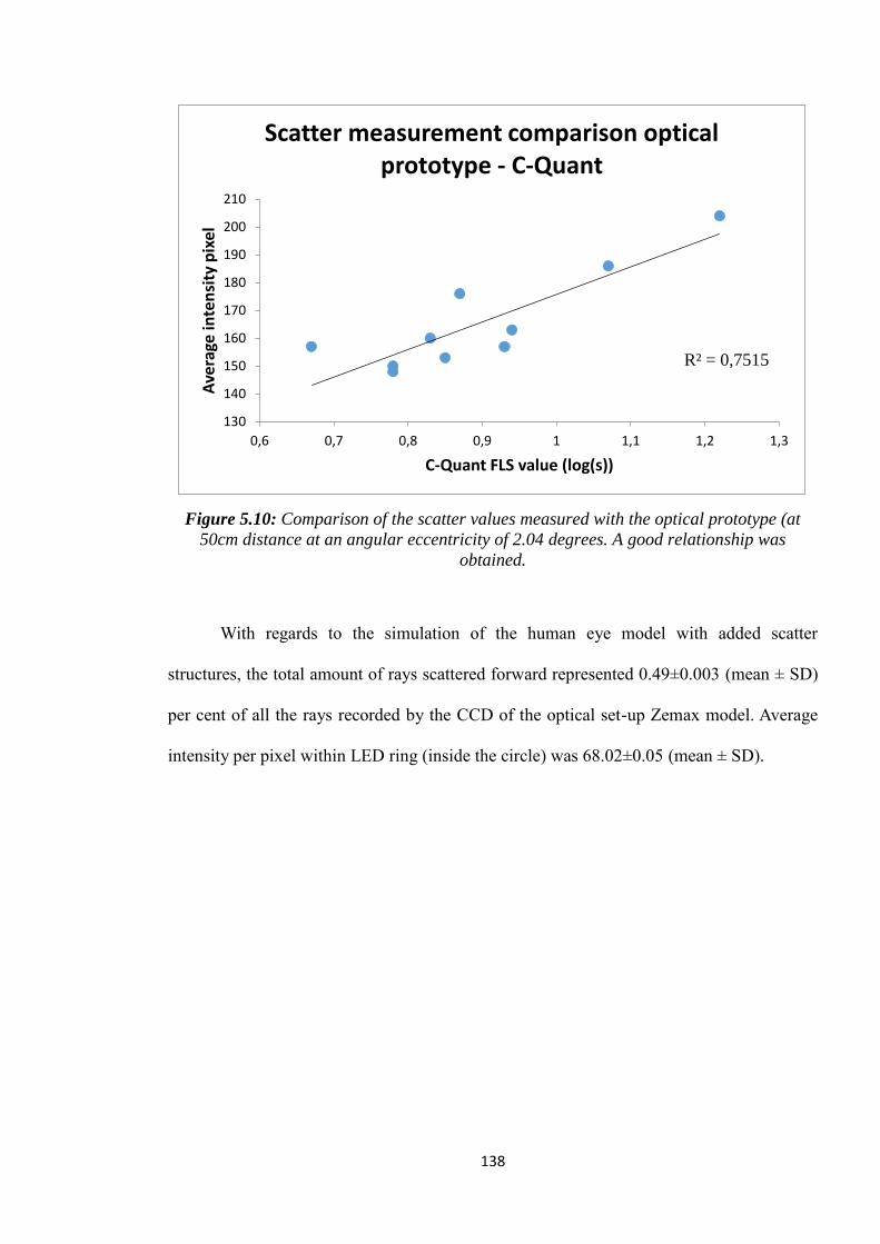
138

Figure 5.10: Comparison of the scatter values measured with the optical prototype (at

50cm distance at an angular eccentricity of 2.04 degrees. A good relationship was

obtained.

With regards to the simulation of the human eye model with added scatter

structures, the total amount of rays scattered forward represented 0.49±0.003 (mean ± SD)

per cent of all the rays recorded by the CCD of the optical set-up Zemax model. Average

intensity per pixel within LED ring (inside the circle) was 68.02±0.05 (mean ± SD).

R² = 0,7515

130

140

150

160

170

180

190

200

210

0,6 0,7 0,8 0,9 1 1,1 1,2 1,3

Ave

rage

inte

nsi

ty p

ixel

C-Quant FLS value (log(s))

Scatter measurement comparison optical prototype - C-Quant

139

5.9 DISCUSSION



The good results obtained from the comparison between the experimental set-up

and the Zemax model validated the optical instrument and allowed for the measurement of

increased levels of light scatter. The results obtained from the measurement of light scatter

from the microscopy plates are in agreement with another previously published study in

which light scatter produced by customized contact lenses was assessed through a double

pass system (De Brouwere et al., 2007). Furthermore, the good results observed in Figure

5.10 allow for the association of measurements to a particular source of scatter (i.e. plate

number and associated microsphere concentration).


COMPARISON RESULTS PROTOTYPE – C-QUANT AND


Results from participants, comparison results prototype – C-Quant

The first results obtained in patients with the experimental set-up are in good

agreement with C-Quant results (r² = 0.75; p < 0.05). The optical set-up is designed to

measure scatter angle as large as psychophysical methods do. These results contradict a

previous study in which the measurement of large angle scatter was limited to

psychophysical methods (Van Den Berg et al., 2009, Benito Lopez et al., 2015). However,

140

they are in agreement with another recent study which utilises an optical method to assess

large angle FLS (Ginis et al., 2012).

In this study, human eyes were tested using the optical set-up and a scatter angle of

2.04⁰ and compared with C-Quant, that measures with an effective eccentricity of 7⁰ (van

den Berg, 1995). Although the differences between the designs of the scatter sources used

by the two instruments must be considered, the agreement obtained with two different

instruments measuring FLS at different scatter angles might be explained in part due to the

definition of the straylight parameter used by C-Quant:

× 𝐹 (van den Berg et al., 2012)

In this formula, the straylight parameter (s) is equal to the scatter angle to the power

of 2 and multiplied by the PSF of the human eye. In this sense, the agreement between the

amounts of FLS measured by the two instruments tested in this study might be explained

by FLS being proportional to the square of the measured scatter angle.

These results suggest that the presented optical set-up could allow measuring

objectively FLS. However, the optical set-up could benefit from several possible

improvements to make it more robust and lead to its application as a clinical instrument.

For instance, a central LED in addition to the LEDs ring light source could be introduced

to match the veiling illuminance created by the LEDs ring and act as an adaptation of the

nulling flickering technique (van den Berg and Ijspeert, 1992). In the classic instrument,

the subject adjusts the luminance of the central light source to match the retinal

illuminance caused by the LEDs ring (van den Berg and Ijspeert, 1992). In this set-up, the

patients input would be replaced by an analysis of the retinal image recorded by the CCD

for different level of luminance of the central LEDs ring. Moreover, in combination with

141

the flicker cancellation technique it would allow the estimation of the full scatter function

of the eye if different scatter angles are measured (Barbur et al., 1993).

Another improvement would be the addition of a system to control the pupillary

diameter while measuring. Short exposures times of the eye to bright lights produce the

activation of the pupil response. Introducing a system that allows for the quick presentation

of the light source to the tested eye and the measurement would avoid the pupil response

(Bergamin and Kardon, 2003). Franssen et al. found that for natural pupils (between 2 and

7 mm of diameter), FLS is weakly affected by the pupillary diameter. However, smaller

pupillary diameters produce a reduction of the measured amount of FLS (Franssen et al.,

2007b).

A critical task while doing the measurements is the alignment of the eye with the

optical system. A small movement of subject´s head can mean a loss of important

information when the LEDs ring image is recorded. The need of an instrument that

automatizes and tests the alignment of the prototype with the tested eye would be of great

benefit. Finally, the lack of a fixation point is another reason for multiple repetitions of

measurements. When the eye is not fixating correctly, the images on the CCD appear

distorted and need to be repeated. In this study, participants were asked to fixate one of the

LEDs from the LED ring, and when the person doing the measurements said, the subject

rapidly fixated on the centre of the ring and the measurement was taken. However, this

method frequently finished with the acquisition of a non-valid image (with artefacts). This

alignment complement would increase the accuracy of the measurement.

Prototype - Zemax scatter eye model

The percentage of FLS obtained from the simulation with the Zemax model of the

human scatter eye is 0.49% and thus lower than the physiologically estimated FLS

142

corresponding to a human eye, which is usually between 1 and 2% (Vos, 1984) of the

incoming light. These results are however in agreement with previous studies in which the

lack of biometric data with respect to corneal scatter parameters was solved by varying the

quantity of scatter structures until FLS in the model agreed with the values calculated by

the CIE (Chen et al., 2012) disability glare formula (Vos and van den Berg, 1999). In this

study (Chen et al., 2012), scatter particles were aimed to mimic the scatter characteristics

of the corneal lens and produce the percentage of light scatter usually attributed to this

lens. In another study, random distributions of particles where added to a model eye trying

to simulate the scatter produced by cataracts in the crystalline lens (Kelly-Pérez et al.,

2011). The lack of biometric data of scatter particles in the eye might explain the results of

the current study (0.49% of FLS rather than 1-2%) where the intensity per pixel obtained in

the model eye was only 68.02±0.05 (mean ± SD) while the average intensity per pixel

measured for the ten participants was 165.4±17.94 (mean ± SD).

In view of our results and previous studies (Kelly-Pérez et al., 2011, Chen et al.,

2012) a first step for achieving a more realistic simulation of intraocular light scatter could

be to increase the complexity of the model (e.g. shape, multiple sizes, locations of scatter

structures) and to be able to insert these elements into an optical design program (basically

creating custom object libraries with Zemax or CAD models). Unfortunately, such steps

would further increase the difficulty of associating an experimental measurement to a

scatter parameter of the model.

In summary, the presented optical set-up has been validated as an objective method

to assess large angle FLS. The FLS measurements from the optical set-up can also be

related to physical parameters through the Zemax model (e.g. scatter particle density).

143

Human eyes large angle FLS measurements from the optical set-up were highly

correlated with data obtained with C-Quant. However, they cannot yet be explained by the

developed Zemax model of the human eye.

144

6. FINAL SUMMARY AND FUTURE WORK

6.1 FINAL SUMMARY

The measurement of the effect of intraocular forward light scatter in the human eye

has been the main motivation of this project. The main effect of forward light scatter on

vision is the decrease of contrast on the retinal image. This reduced contrast may become a

significant issue, particularly when a good visual performance is not only required but

obligatory (e.g. plane pilot).

This PhD thesis started with the comparison between the instrument considered the

current gold standard to measure FLS (C-Quant) and its predecessor (the Van der Berg

Straylight meter) (chapter 2). Despite the importance of the two instruments in the

literature, the relationship between measurements obtained with the two techniques had

never been quantified. Results from our study are slightly surprising since no significant

relationship could be found between the two measurements (even with a multivariable

function; chapter 2) but illustrate the difficulty in quantifying precisely FLS and the

importance of the angular domain.

Following this study, we took interest in commercial instruments (Hartmann-Shack

in chapter 3 and Pentacam in chapter 4) by measuring FLS and BLS. The work presented

in chapter 3 allowed us to clarify the relation between FLS assessed with the C-Quant and

FLS assessed from Hartmanngrams to demonstrate that a commercial Hartmann-Shack

wavefront sensor cannot be used to assess FLS without significant modifications. The

work presented in chapter 4, allowed us to illustrate the lack of direct correlation between

forward and backward scattering

145

Finally, an innovative prototype to measure objectively the FLS in the eye together

with its Zemax model is presented in chapter 5. This optical prototype is tested on a model

eye as well as a human eye. Scatter measurements obtained with this prototype are

comparable to the ones obtained with the C-Quant straylight meter. A Zemax scatter model

of the eye is also presented in this chapter but the simplicity of the model lead to a lack of

agreement between the model and real FLS data obtained with the prototype.

6.2 FUTURE WORK

Objective forward light scattering assessment through Hartmann-Shack

aberrometer spot patterns: As described in chapter 3, commercial Hartmann-Shack

aberrometers usually incorporate a confocal aperture to reduce high angle scatter

that increases the sensor‟s performance (Donnelly Iii et al., 2004), but limits the

measurement of light scatter in a human eye. The study presented in chapter 3

might give different results if scatter measurements are obtained from an

aberrometer that has been modified in this way to receive the maximum amount of

scatter light from the human eye. In addition, a patent presenting a method to assess

the scatter from the space situated between the PSF lets of a Hartmann-Shack spot

pattern has been presented (Levecq and Harms, 2011) and that could possibly be of

interest in order to give an additional application to aberrometers by assessing

intraocular forward scatter.

Prototype for the objective measurement of forward light scattering: Improvements

and future research for this prototype have already been outlined in chapter 5. After

such improvements, many different studies can be performed in order to validate

146

the instrument for human eyes in a great variety of situations (e.g. different cataract

grades or ocular diseases), for different age groups and wavelengths, but also to

assess the effect of some topical and intraocular drugs.

Human eye model of intraocular scatter: Scatter sources within the ocular media

that are described in the current literature cannot explain the amount of forward

light scatter attributed to a healthy eye (1-2%) as shown in chapter 5. Deeper

understanding of the scatter characteristics of the human eye could be provided

with a model of the human eye for intraocular scatter that simulates the different

eye clinical cases and their evolution. This model could include different types of

intraocular structures, with different shapes and sizes that mimic in a more realistic

way the scattering complexity of the human eye. The eye model presented in

chapter 5 was developed in Zemax but could also have been developed in a

specially developed modelling software for the eye that might introduce some

scatter modelling advantages (Donnelly, 2008).

147

7. REFERENCES

AGUIRRE, R., COLOMBO, E., ISSOLIO, L., LUQUE, S., VILASECA, M. & PUJOL, J.

2007. Reaction times and threshold contrast in the measurement of intraocular scattering

and glare. Optica Pura y Aplicada, 40, 111-117.

ALLEN, M. J. & VOS, J. J. 1967. Ocular scattered light and visual performance as a

function of age. Am J Optom Arch Am Acad Optom, 44, 717-27.

APPLEGATE, R. A. & WOLF, M. 1987. Disability glare increased by hydrogel lens wear.

Am J Optom Physiol Opt, 64, 309-12.

APPLEGATE, R. A., PESUDOVS, K., MARSACK, J. D. & DONNELLY III, W. J. 2004.

Optical quality metrics of backscatter, foward scatter and wave aberration account for over

50% of the variance in low luminance high contrast visual acuity in cataract patients with

nuclear opalescence. Invest. Ophthalmol. Vis. Sci., 45, 1747-.

APPLEGATE RA, T., L.N. 2003. Methods and systems for measuring local scattering and

aberration properties of optical media. US Patent.

APPLEGATE RA, T. L. 2000. Localized measurement of scatter due to cataract.

Investigative Ophthalmology and Visual Science, 41, Abstract 13.

ARTAL, P., MARCOS, S., NAVARRO, R. & WILLIAMS, D. R. 1995. Odd aberrations

and double-pass measurements of retinal image quality. Journal of the Optical Society of

America A: Optics and Image Science, and Vision, 12, 195-201.

ARTAL, P., GUIRAO, A., BERRIO, E. & WILLIAMS, D. R. 2001a. Compensation of

corneal aberrations by the internal optics in the human eye. Journal of Vision, 1, 1-8.

ARTAL, P., GUIRAO, A., BERRIO, E. & WILLIAMS, D. R. 2001b. Compensation of

corneal aberrations by the internal optics in the human eye. J Vis, 1, 1-8.

ASLAM, T. M., HAIDER, D. & MURRAY, I. J. 2007. Principles of disability glare

measurement: an ophthalmological perspective. Acta Ophthalmol Scand, 85, 354-60.

148

BABIZHAYEV, M. A., DEYEV, A. I., YERMAKOVA, V. N., DAVYDOVA, N. G.,

KURYSHEVA, N. I., DOROSHENKO, V. S. & ZHUKOTSKII, A. V. 2003. Image analysis

and glare sensitivity in human age-related cataracts. Clin Exp Optom, 86, 157-72.

BAILEY, I. L. & BULLIMORE, M. A. 1991. A new test for the evaluation of disability

glare. Optom Vis Sci, 68, 911-7.

BAL, T., COECKELBERGH, T., VAN LOOVEREN, J., ROZEMA, J. J. & TASSIGNON,

M. J. 2011. Influence of cataract morphology on straylight and contrast sensitivity and its

relevance to fitness to drive. Ophthalmologica, 225, 105-11.

BARBUR, J. L., CUNHA, D. D., HARLOW, A. & WOODWARD, E. G. 1993. Methods

for the measurement and analysis of light scattered in the human eye. In: AMERICA, O. S.

O. (ed.).

BARBUR, J. L., EDGAR, D. F. & WOODWARD, E. G. 1995. Measurement of the

scattering characteristics of the eye in relation to pupil size. Journal of the Optical Society

of America. A, Optics and image science, 250-253.

BARBUR, J. L., WEISKRANTZ, L. & HARLOW, J. A. 1999. The unseen color aftereffect

of an unseen stimulus: Insight from blindsight into mechanisms of color afterimages.

Proceedings of the National Academy of Sciences of the United States of America, 96,

11637-11641.

BENEDEK, G. B. 1971. Theory of transparency of the eye. Appl Opt, 10, 459-73.

BENITO LOPEZ, P., RADHAKRISHNAN, H. & NOURRIT, V. 2014. Comparison of the

compensation comparison method and the direct compensation method for straylight

measurement. Proceedings of the VII European/ I World Meeting in Visual and

Physiological Optics VPOptics 2014. Robert Iskander and Henryk T. Kasprzak. ed.

Wroclaw (Poland): Drukarnia Oficyny Wydawniczej Politechniki Wrocławskiej.

BENITO LOPEZ, P., RADHAKRISHNAN, H. & NOURRIT, V. 2015. Comparison of

forward light scatter estimations using Shack-Hartmann spot patterns and a straylight

meter. J Cataract Refract Surg, 41, 320-6.

149

BERGAMIN, O. & KARDON, R. H. 2003. Latency of the pupil light reflex: sample rate,

stimulus intensity, and variation in normal subjects. Invest Ophthalmol Vis Sci, 44, 1546-

54.

BERGEVIN, J. & MILLODOT, M. 1967. Glare with ophthalmic and corneal lenses. Am J

Optom Arch Am Acad Optom, 44, 213-21.

BETTELHEIM, F. A. & ALI, S. 1985. Light scattering of normal human lens. III.

Relationship between forward and back scatter of whole excised lenses. Exp Eye Res, 41,

1-9.

BLAND, J. M. & ALTMAN, D. G. 1986. Statistical methods for assessing agreement

between two methods of clinical measurement. Lancet, 1, 307-10.

BLAND, J. M. & ALTMAN, D. G. 1999. Measuring agreement in method comparison

studies. Stat Methods Med Res, 8, 135-60.

BOHREN, C. F. & HUFFMAN, D. R. 2007. Absorption and Scattering of Light by Small

Particles. Wiley-VCH Verlag GmbH.

BORN, M. & WOLF, E. 1980. Principles of Optics, New York, Pergamon Press.

BUENO, J. M., BERRIO, E., OZOLINSH, M. & ARTAL, P. 2004. Degree of polarization

as an objective method of estimating scattering. J Opt Soc Am A Opt Image Sci Vis, 21,

1316-21.

BUENO, J. M., DE BROUWERE, D., GINIS, H., SGOUROS, I. & ARTAL, P. 2007.

Purkinje imaging system to measure anterior segment scattering in the human eye. Opt

Lett, 32, 3447-9.

CASTILLA-MARTI, M., VAN DEN BERG, T. J. & DE SMET, M. D. 2015. EFFECT OF

VITREOUS OPACITIES ON STRAYLIGHT MEASUREMENTS. Retina, 35 (6):1240-6.

CERVINO, A., MONTES-MICO, R. & FERRER-BLASCO, T. 2008a. Reliability results

of straylight measurements using the C-Quant. Acta Ophthalmologica, 86, 0-0.

CERVIÑO, A., BANSAL, D., HOSKING, S. L. & MONTÉS-MICÓ, R. 2008b. Objective

measurement of intraocular forward light scatter using Hartmann-Shack spot patterns from

150

clinical aberrometers. Model-eye and human-eye study. Journal of Cataract and Refractive

Surgery, 34, 1089-1095.

CERVIÑO, A., MONTES-MICO, R. & HOSKING, S. L. 2008c. Performance of the

compensation comparison method for retinal straylight measurement: Effect of patient's

age on repeatability. British Journal of Ophthalmology, 92, 788-791.

COOPENS, J. E., FRANSSEN, L. & VAN DEN BERG, T. J. T. P. 2006. Reliability of the

compensation comparison method for measuring retinal stray light studied using Monte-

Carlo simulations. Journal of Biomedical Optics, 11.COPPENS, J. E., FRANSSEN, L. &

VAN DEN BERG, T. J. 2006a. Wavelength dependence of intraocular straylight. Exp Eye

Res, 82, 688-92.

COPPENS, J. E., FRANSSEN, L., VAN RIJN, L. J. & VAN DEN BERG, T. J. T. P. 2006b.

Reliability of the compensation comparison stray-light measurement method. Journal of

Biomedical Optics, 11.

COREN, S. & GIRGUS, J. S. 1972. Density of human lens pigmentation: in vivo measures

over an extended age range. Vision Res, 12, 343-6.

COSTELLO, M. J., JOHNSEN, S., GILLILAND, K. O., FREEL, C. D. & FOWLER, W.

C. 2007. Predicted light scattering from particles observed in human age-related nuclear

cataracts using mie scattering theory. Invest Ophthalmol Vis Sci, 48, 303-12.

COX, M. J., ATCHISON, D. A. & SCOTT, D. H. 2003. Scatter and its implications for the

measurement of optical image quality in human eyes. Optom Vis Sci, 80, 58-68.

CHARMAN, W. N. 1991. Wavefront aberration of the eye: a review. Optom Vis Sci, 68,

574-83.

CHARMAN, W. N. 1991b. Optics of the Human Eye. In. Vision and Visual Dysfunction.

Visual Optics and Instrumentation, London Macmillan.

CHEN, Y. C., JIANG, C. J., YANG, T. H. & SUN, C. C. 2012. Development of a human

eye model incorporated with intraocular scattering for visual performance assessment. J

Biomed Opt, 17, 075009.

151

CHISHOLM, C. 2003. Assessment of visual performance: Comparison of normal subjects

and post-refractive surgery patients. Doctor in Philosophy, City University.

CHYLACK, L. T., JR., WOLFE, J. K., SINGER, D. M., LESKE, M. C., BULLIMORE,

M. A., BAILEY, I. L., FRIEND, J., MCCARTHY, D. & WU, S. Y. 1993. The Lens

Opacities Classification System III. The Longitudinal Study of Cataract Study Group. Arch

Ophthalmol, 111, 831-6.

DE BROUWERE, D., GINIS, H. S., VAN DEN BERG, T. & PALLIKARIS, I. 2007.

Comparative Study of Optical and Psychophysical Measurements for Intraocular Scatter

Using Calibrated Scattering Contact Lenses. Invest. Ophthalmol. Vis. Sci. , 48, 6006-.

DE WAARD, P. W. T., IJSPEERT, J. K., VAN DEN BERG, T. J. T. P. & DE JONG, P. T. V.

M. 1992. Intraocular light scattering in age-related cataracts. Investigative Ophthalmology

and Visual Science, 33, 618-625.

DE WIT, G. C. & COPPENS, J. E. 2003. Stray light of spectacle lenses compared with

stray light in the eye. Optom Vis Sci, 80, 395-400.

DELAYE, M. & TARDIEU, A. 1983. Short-range order of crystallin proteins accounts for

eye lens transparency. Nature, 302, 415-7.

DELORI, F. C. 2004. Autofluorescence method to measure macular pigment optical

densities fluorometry and autofluorescence imaging. Arch Biochem Biophys, 430, 156-62.

DEMOTT, D. W. & BOYNTON, R. M. 1958. Retinal distribution of entoptic stray light. J

Opt Soc Am, 48, 13-22.

DIAZ-VALLE, D., ARRIOLA-VILLALOBOS, P., GARCIA-VIDAL, S. E., SANCHEZ-

PULGARIN, M., BORREGO SANZ, L., GEGUNDEZ-FERNANDEZ, J. A. & BENITEZ-

DEL-CASTILLO, J. M. 2012. Effect of lubricating eyedrops on ocular light scattering as a

measure of vision quality in patients with dry eye. J Cataract Refract Surg, 38, 1192-7.

DONNELLY III, W. J., PESUDOVS, K., MARSACK, J. D., SARVER, E. J. &

APPLEGATE, R. A. 2004. Quantifying scatter in Shack-Hartmann images to evaluate

nuclear cataract. Journal of Refractive Surgery, 20, S515-S522.

152

DONNELLY III, W. J. & APPLEGATE, R. A. 2005. Influence of exposure time and pupil

size on a Shack-Hartmann metric of forward scatter. Journal of Refractive Surgery, 21,

S547-S551.

DONNELLY, W., 3RD 2008. The Advanced Human Eye Model (AHEM): a personal

binocular eye modeling system inclusive of refraction, diffraction, and scatter. J Refract

Surg, 24, 976-83.

DONNELLY, W. J., 3RD, PESUDOVS, K., MARSACK, J. D., SARVER, E. J. &

APPLEGATE, R. A. 2004. Quantifying scatter in Shack-Hartmann images to evaluate

nuclear cataract. J Refract Surg, 20, S515-22.

DONNELLY, W. J., 3RD & APPLEGATE, R. A. 2005. Influence of exposure time and

pupil size on a Shack-Hartmann metric of forward scatter. J Refract Surg, 21, S547-51.

DREWS, R. C. 1964. DEPTH OF FIELD IN SLIT LAMP PHOTOGRAPHY. An optical

solution using the scheimpflug principle. Ophthalmologica, 148, 143-50.

DUBBELMAN, M. & VAN DER HEIJDE, G. L. 2001. The shape of the aging human

lens: curvature, equivalent refractive index and the lens paradox. Vision Res, 41, 1867-77.

DUBBELMAN, M., VAN DER HEIJDE, G. L. & WEEBER, H. A. 2001. The thickness of

the aging human lens obtained from corrected Scheimpflug images. Optom Vis Sci, 78,

411-6.

DUBBELMAN, M., SICAM, V. A. & VAN DER HEIJDE, G. L. 2006. The shape of the

anterior and posterior surface of the aging human cornea. Vision Res, 46, 993-1001.

ELFLEIN, H. M., HOFHERR, T., BERISHA-RAMADANI, F., WEYER, V., LAMPE, C.,

BECK, M. & PITZ, S. 2013. Measuring corneal clouding in patients suffering from

mucopolysaccharidosis with the Pentacam densitometry programme. Br J Ophthalmol, 97,

829-33.

ELLIOTT, D. B., MITCHELL, S. & WHITAKER, D. 1991. Factors affecting light scatter

in contact lens wearers. Optom Vis Sci, 68, 629-33.

ELLIOTT, D. B. & BULLIMORE, M. A. 1993. Assessing the reliability, discriminative

ability, and validity of disability glare tests. Invest Ophthalmol Vis Sci, 34, 108-19.

153

ELLIOTT, D. B., FONN, D., FLANAGAN, J. & DOUGHTY, M. 1993a. Relative

sensitivity of clinical tests to hydrophilic lens-induced corneal thickness changes. Optom

Vis Sci, 70, 1044-8.

ELLIOTT, D. B., YANG, K. C., DUMBLETON, K. & CULLEN, A. P. 1993b. Ultraviolet-

induced lenticular fluorescence: intraocular straylight affecting visual function. Vision Res,

33, 1827-33.

FLAMANT, M. F. 1955. "Étude de la repartition de lumière dans l'image retinienne d'une

fente," Rev. Optical Engineering, 433-459.

FRANSSEN, L., COPPENS, J. E. & VAN DEN BERG, T. J. T. P. 2006. Compensation

comparison method for assessment of retinal straylight. Investigative Ophthalmology and

Visual Science, 47, 768-776.

FRANSSEN, L., COPPENS, J. E. & VAN DEN BERG, T. J. 2007a. Modulation depth

threshold in the Compensation Comparison approach. J Vis, 7, 8.

FRANSSEN, L., TABERNERO, J., COPPENS, J. E. & VAN DEN BERG, T. J. 2007.

Pupil size and retinal straylight in the normal eye. Invest Ophthalmol Vis Sci, 48, 2375-82.

FREUND, D. E., MCCALLY, R. L. & FARRELL, R. A. 1986. Effects of fibril orientations

on light scattering in the cornea. J Opt Soc Am A, 3, 1970-82.

FRY, G. A. & ALPERN, M. 1953b. The effect of a peripheral glare source upon the

apparent brightness of an object. J Opt Soc Am, 43, 189-95.

FUJISAWA, K. & SASAKI, K. 1995. Changes in light scattering intensity of the

transparent lenses of subjects selected from population-based surveys depending on age:

analysis through Scheimpflug images. Ophthalmic Res, 27, 89-101.

FYODOROV, S. N. & DURNEV, V. V. 1979. Operation of dosaged dissection of corneal

circular ligament in cases of myopia of mild degree. Ann Ophthalmol, 11, 1885-90.

GARTRY, D. S., KERR MUIR, M. G. & MARSHALL, J. 1992. Excimer laser

photorefractive keratectomy. 18-month follow-up. Ophthalmology, 99, 1209-19.

GEORGE, S. 2005. Scatter in the eye. The eye and the light.

154

GILLILAND, K. O., FREEL, C. D., LANE, C. W., FOWLER, W. C. & COSTELLO, M. J.

2001. Multilamellar bodies as potential scattering particles in human age-related nuclear

cataracts. Mol Vis, 7, 120-30.

GILLILAND, K. O., FREEL, C. D., JOHNSEN, S., CRAIG FOWLER, W. &

COSTELLO, M. J. 2004. Distribution, spherical structure and predicted Mie scattering of

multilamellar bodies in human age-related nuclear cataracts. Exp Eye Res, 79, 563-76.

GILLILAND, K. O., JOHNSEN, S., METLAPALLY, S., COSTELLO, M. J.,

RAMAMURTHY, B., KRISHNA, P. V. & BALASUBRAMANIAN, D. 2008. Mie light

scattering calculations for an Indian age-related nuclear cataract with a high density of

multilamellar bodies. Mol Vis, 14, 572-82.

GINIS, H., PÉREZ, G. M., BUENO, J. M. & ARTAL, P. 2012b. The wide-angle point

spread function of the human eye reconstructed by a new optical method. Journal of

Vision, 12, 1-10.

GINIS, H. S., PEREZ, G. M., BUENO, J. M., PENNOS, A. & ARTAL, P. 2013.

Wavelength Dependence of the Ocular Straylight. Investigative Ophthalmology & Visual

Science, 54, 3702-3708.

GREENSTEIN, S. A., FRY, K. L., BHATT, J. & HERSH, P. S. 2010. Natural history of

corneal haze after collagen crosslinking for keratoconus and corneal ectasia: Scheimpflug

and biomicroscopic analysis. J Cataract Refract Surg, 36, 2105-14.

GROVER, S., ALEXANDER, K. R., CHOI, D. M. & FISHMAN, G. A. 1998. Intraocular

light scatter in patients with choroideremia. Ophthalmology, 105, 1641-5.

GUIRAO, A., GONZALEZ, C., REDONDO, M., GERAGHTY, E., NORRBY, S. &

ARTAL, P. 1999. Average optical performance of the human eye as a function of age in a

normal population. Invest Ophthalmol Vis Sci, 40, 203-13.

GUTIERREZ, R., JIMENEZ, J. R., VILLA, C., VALVERDE, J. A. & ANERA, R. G. 2003.

Simple device for quantifying the influence of halos after lasik surgery. J Biomed Opt, 8,

663-7.

155

HAHNEL, C., SOMODI, S., WEISS, D. G. & GUTHOFF, R. F. 2000. The keratocyte

network of human cornea: a three-dimensional study using confocal laser scanning

fluorescence microscopy. Cornea, 19, 185-93.

HANSON, S. R., HASAN, A., SMITH, D. L. & SMITH, J. B. 2000. The major in vivo

modifications of the human water-insoluble lens crystallins are disulfide bonds,

deamidation, methionine oxidation and backbone cleavage. Exp Eye Res, 71, 195-207.

HART, R. W. & FARRELL, R. A. 1969. Light Scattering in the Cornea. Journal of the

Optical Society of America, 59, 766-773.

HEMENGER, R. P. 1992. Sources of intraocular light scatter from inversion of an

empirical glare function. Appl Opt, 31, 3687-93.

HENNELLY, M. L., BARBUR, J. L., EDGAR, D. F. & WOODWARD, E. G. 1998. The

effect of age on the light scattering characteristics of the eye. Ophthalmic and

Physiological Optics, 18, 197-203.

HESS, R. F., WOO, G. C. & WHITE, P. D. 1985. Contrast attenuation characteristics of

iris clipped intraocular lens implants in situ. British Journal of Ophthalmology, 69, 129-

135.

HILLENAAR, T., CALS, R. H., EILERS, P. H., WUBBELS, R. J., VAN

CLEYNENBREUGEL, H. & REMEIJER, L. 2011. Normative database for corneal

backscatter analysis by in vivo confocal microscopy. Invest Ophthalmol Vis Sci, 52, 7274-

81.

HODGKINSON, I. J., GREER, P. B. & MOLTENO, A. C. 1994. Point-spread function for

light scattered in the human ocular fundus. J Opt Soc Am A Opt Image Sci Vis, 11, 479-86.

HOGAN, M. J., ALVARADO, J. A. & WEDDELL, J. E. 1971. Histology of the human

eye; an atlas and textbook, Philadelphia, Saunders.

HOLLADAY, J. T., PRAGER, T. C., TRUJILLO, J. & RUIZ, R. S. 1987. Brightness acuity

test and outdoor visual acuity in cataract patients. J Cataract Refract Surg, 13, 67-9.

HOLLADAY, L. L. 1926a. THE FUNDAMENTALS OF GLARE AND VISIBILITY.

Journal of the Optical Society of America, 12, 271-319.

156

HOLLADAY, L. L. 1926b. The fundamentals of glare and visibility. J. Opt. Soc. Am., 12,

271-319.

JESTER, J. V., MOLLER-PEDERSEN, T., HUANG, J., SAX, C. M., KAYS, W. T.,

CAVANGH, H. D., PETROLL, W. M. & PIATIGORSKY, J. 1999. The cellular basis of

corneal transparency: evidence for 'corneal crystallins'. J Cell Sci, 112 ( Pt 5), 613-22.

JESTER, J. V., LEE, Y. G., HUANG, J., HOUSTON, J., ADAMS, B., CAVANAGH, H. D.

& PETROLL, W. M. 2007. Postnatal corneal transparency, keratocyte cell cycle exit and

expression of ALDH1A1. Invest Ophthalmol Vis Sci, 48, 4061-9.

JESTER, J. V. 2008a. Corneal crystallins and the development of cellular transparency.

Seminars in Cell and Developmental Biology, 19, 82-93.

JINABHAI, A., O'DONNELL, C., RADHAKRISHNAN, H. & NOURRIT, V. 2012.

Forward light scatter and contrast sensitivity in keratoconic patients. Cont Lens Anterior

Eye, 35, 22-7.

KASTHURIRANGAN, S., MARKWELL, E. L., ATCHISON, D. A. & POPE, J. M. 2008.

In vivo study of changes in refractive index distribution in the human crystalline lens with

age and accommodation. Invest Ophthalmol Vis Sci, 49, 2531-40.

KELLY-PEREZ, I., BRUCE, N. C., BERRIEL-VALDOS, L. R., WERNER, A. &

DELGADO ATENCIO, J. A. 2013. Computational model of the effect of light scattering

from cataracts in the human eye. J Opt Soc Am A Opt Image Sci Vis, 30, 2585-94.

KELLY-PÉREZ, I., BRUCE, N. C. & BERRIEL-VALDOS, L. R. Modelling image

formation on the retina and backscattered light in the human eye with cataracts. 2011.

800136-800136-8.

KERKER, M. 1969. The Scattering of Light and Other Electromagnetic Radiation, New

York, Academic Press.

KIRKWOOD, B. J., HENDICOTT, P. L., READ, S. A. & PESUDOVS, K. 2009.

Repeatability and validity of lens densitometry measured with Scheimpflug imaging. J

Cataract Refract Surg, 35, 1210-5.

157

KOENZ, F., RICKA, J., FRENZ, M. & FANKHAUSER, F. 1995. Dynamic light scattering

in the vitreous: performance of the single-mode fiber technique. Optical Engineering, 34,

2390-2395.

KOH, S., MAEDA, N., IKEDA, C., ASONUMA, S., MITAMURA, H., OIE, Y., SOMA,

T., TSUJIKAWA, M., KAWASAKI, S. & NISHIDA, K. 2014. Ocular forward light

scattering and corneal backward light scattering in patients with dry eye. Invest

Ophthalmol Vis Sci, 55, 6601-6.

KURODA, T., FUJIKADO, T., MAEDA, N., OSHIKA, T., HIROHARA, Y. & MIHASHI,

T. 2002. Wavefront analysis in eyes with nuclear or cortical cataract. American Journal of

Ophthalmology, 134, 1-9.

LAPID-GORTZAK, R., VAN DER LINDEN, J. W., VAN DER MEULEN, I. J.,

NIEUWENDAAL, C. P., MOURITS, M. P. & VAN DEN BERG, T. J. 2010. Straylight

before and after hyperopic laser in situ keratomileusis or laser-assisted subepithelial

keratectomy. J Cataract Refract Surg, 36, 1919-24.

LECLAIRE, J., NADLER, M. P., WEISS, S. & MILLER, D. 1982. A new glare tester for

clinical testing. Results comparing normal subjects and variously corrected aphakic

patients. Arch Ophthalmol, 100, 153-8.

LEROUX, C. & DAINTY, C. 2010. Estimation of centroid positions with a matched-filter

algorithm: relevance for aberrometry of the eye. Opt Express, 18, 1197-206.

LEVECQ, X. J. F. & HARMS, F. 2011. Method and device for measuring the local

scattering of an optical system. Google Patents.

LIANG, J., GRIMM, B., GOELZ, S. & BILLE, J. F. 1994. Objective measurement of

wave aberrations of the human eye with the use of a Hartmann-Shack wave-front sensor. J

Opt Soc Am A Opt Image Sci Vis, 11, 1949-57.

LIANG, J. & WESTHEIMER, G. 1995. Optical performances of human eyes derived from

double-pass measurements. J Opt Soc Am A Opt Image Sci Vis, 12, 1411-6.

158

LIM, D. H., KIM, T. H., CHUNG, E.-S. & CHUNG, T.-Y. 2014. Measurement of lens

density using Scheimpflug imaging system as a screening test in the field of health

examination for age-related cataract. British Journal of Ophthalmology.

LIOU, H. L. & BRENNAN, N. A. 1997. Anatomically accurate, finite model eye for

optical modeling. J Opt Soc Am A Opt Image Sci Vis, 14, 1684-95.

LOHMANN, C. P., GARTRY, D. S., MUIR, M. K., TIMBERLAKE, G. T., FITZKE, F. W.

& MARSHALL, J. 1991. Corneal haze after excimer laser refractive surgery: objective

measurements and functional implications. Eur J Ophthalmol, 1, 173-80.

LOHMANN, C. P., FITZKE, F., O'BRART, D., MUIR, M. K., TIMBERLAKE, G. &

MARSHALL, J. 1993. Corneal light scattering and visual performance in myopic

individuals with spectacles, contact lenses, or excimer laser photorefractive keratectomy.

Am J Ophthalmol, 115, 444-53.

LOPEZ-GIL, N. & ARTAL, P. 1997. Comparison of double-pass estimates of the retinal-

image quality obtained with green and near-infrared light. J Opt Soc Am A Opt Image Sci

Vis, 14, 961-71.

LOVICU, F. J. & ROBINSON, M. L. 2004. Development of the Ocular Lens, Cambridge

University Press.

MAGALHAES, F. P., COSTA, E. F., CARIELLO, A. J., RODRIGUES, E. B. &

HOFLING-LIMA, A. L. 2011. Comparative analysis of the nuclear lens opalescence by the

Lens Opacities Classification System III with nuclear density values provided by Oculus

Pentacam: a cross-section study using Pentacam Nucleus Staging software. Arq Bras

Oftalmol, 74, 110-3.

MALDONADO, M. J., ARNAU, V., NAVEA, A., MARTINEZ-COSTA, R., MICO, F. M.,

CISNEROS, A. L. & MENEZO, J. L. 1996. Direct objective quantification of corneal haze

after excimer laser photorefractive keratectomy for high myopia. Ophthalmology, 103,

1970-8.

MARTIN, L. 1999. Computerized method to measure glare and contrast sensitivity in

cataract patients. J Cataract Refract Surg, 25, 411-5.

159

MAS, D., ESPINOSA, J., DOMENECH, B., PEREZ, J., KASPRZAK, H. & ILLUECA, C.

2009. Correlation between the dioptric power, astigmatism and surface shape of the

anterior and posterior corneal surfaces. Ophthalmic Physiol Opt, 29, 219-26.

MAURICE, D. M. 1957. The structure and transparency of the cornea. The Journal of

Physiology, 136, 263-286.1.

MAURICE, D. M. 1969. The cornea and sclera. In the eye, 1, 489-600.

MCCALLY & FARRELL 1988. Interaction of light and the cornea: light scattering versus

transparency. The Cornea: Transactions of the World Congress on the Cornea III. New

York: Raven Press Ltd.

MCDONALD, M. B., KAUFMAN, H. E., FRANTZ, J. M., SHOFNER, S., SALMERON,

B. & KLYCE, S. D. 1989. Excimer laser ablation in a human eye. Case report. Arch


MCLAREN, J. W., NAU, C. B., KITZMANN, A. S. & BOURNE, W. M. 2005. Keratocyte

density: comparison of two confocal microscopes. Eye Contact Lens, 31, 28-33.

MEACOCK, W. R., SPALTON, D. J., BOYCE, J. & MARSHALL, J. 2003. The Effect of

Posterior Capsule Opacification on Visual Function. Investigative Ophthalmology and

Visual Science, 44, 4665-4669.

MEEK, K. M., TUFT, S. J., HUANG, Y., GILL, P. S., HAYES, S., NEWTON, R. H. &

BRON, A. J. 2005. Changes in collagen orientation and distribution in keratoconus

corneas. Invest Ophthalmol Vis Sci, 46, 1948-56.

MICHAEL, R., VAN RIJN, L. J., VAN DEN BERG, T. J. T. P., BARRAQUER, R. I.,

GRABNER, G., WILHELM, H., COECKELBERGH, T., EMESZ, M., MARVAN, P. &

NISCHLER, C. 2009b. Association of lens opacities, intraocular straylight, contrast

sensitivity and visual acuity in European drivers. Acta Ophthalmologica, 87, 666-671.

MIE, G. 1908. Beiträge zur Optik trüber Medien, speziell kolloidaler Metallösungen.

Annalen der Physik, 330, 377-445.

160

MIHASHI, T., HIROHARA, Y., BESSHO, K., MAEDA, N., OSHIKA, T. & FUJIKADO,

T. 2006. Intensity analysis of Hartmann-Shack images in cataractous, keratoconic, and

normal eyes to investigate light scattering. Jpn J Ophthalmol, 50, 323-33.

MILLER, D., JERNIGAN, M. E., MOLNAR, S., WOLF, E. & NEWMAN, J. 1972a.

Laboratory evaluation of a clinical glare tester. Archives of Ophthalmology, 87, 324-332.

MILLER, J., WILSON, W. S., WILSON, C. G. & UTTAMCHANDANI, D. 2005.

Minimally invasive, direct, real time measurement of drug concentration in the anterior

eye. The British Journal of Ophthalmology, 89, 1147-1151.

MIRANDA, M. A., RADHAKRISHNAN, H. & O'DONNELL, C. 2009. Repeatability of

corneal thickness measured using an Oculus Pentacam. Optom Vis Sci, 86, 266-72.

MOLLER-PEDERSEN, T. 1997. A comparative study of human corneal keratocyte and

endothelial cell density during aging. Cornea, 16, 333-8.

MOLLER-PEDERSEN, T. 2004. Keratocyte reflectivity and corneal haze. Exp Eye Res,

78, 553-60.

MONTENEGRO, G. A., MICHAEL, R. & VAN DEN BERG, T. J. 2012. Variation of

straylight between contra lateral eyes - results from 1017 healthy subjects. Acta

Ophthalmol, 90, e332-3.

MONTÉS-MICÓ, R., FERRER-BLASCO, T., CERVIÑO, A., GONZÁLEZ-MÉIJOME, J.

M. & PUCHADES, C. 2008. Clinical use of the ocular point spread function for retinal

image quality assessment. Expert Review of Ophthalmology, 3, 523-527.

NAM, J., THIBOS, L. N., BRADLEY, A., HIMEBAUGH, N. & LIU, H. 2011. Forward

light scatter analysis of the eye in a spatially-resolved double-pass optical system. Opt

Express, 19, 7417-38.

NAVARRO, R. 2009. The Optical Design of the Human Eye: a Critical Review. Journal of

Optometry, 2, 3-18.

NI DHUBHGHAILL, S., ROZEMA, J. J., JONGENELEN, S., RUIZ HIDALGO, I.,

ZAKARIA, N. & TASSIGNON, M. J. 2014. Normative values for corneal densitometry

analysis by Scheimpflug optical assessment. Invest Ophthalmol Vis Sci, 55, 162-8.

161

NIETO-BONA, A., LORENTE-VELAZQUEZ, A., COLLAR, C. V., NIETO-BONA, P. &

MESA, A. G. 2010. Intraocular straylight and corneal morphology six months after

LASIK. Curr Eye Res, 35, 212-9.

NIO, Y. K., JANSONIUS, N. M., WIJDH, R. H., BEEKHUIS, W. H., WORST, J. G.,

NORRBY, S. & KOOIJMAN, A. C. 2003. Effect of methods of myopia correction on

visual acuity, contrast sensitivity, and depth of focus. J Cataract Refract Surg, 29, 2082-95.

NISCHLER, C., MICHAEL, R., WINTERSTELLER, C., MARVAN, P., EMESZ, M.,

VAN RIJN, L. J., VAN DEN BERG, T. J., WILHELM, H., COECKELBERGH, T.,

BARRAQUER, R. I., GRABNER, G. & HITZL, W. 2010. Cataract and pseudophakia in

elderly European drivers. Eur J Ophthalmol, 20, 892-901.

NORREN, D. V. & VOS, J. J. 1974. Spectral transmission of the human ocular media.

Vision Res, 14, 1237-44.

O'BRART, D. P., LOHMANN, C. P., FITZKE, F. W., KLONOS, G., CORBETT, M. C.,

KERR-MUIR, M. G. & MARSHALL, J. 1994. Discrimination between the origins and

functional implications of haze and halo at night after photorefractive keratectomy. J

Refract Corneal Surg, 10, S281.

OLSEN, T. 1982. Light scattering from the human cornea. Invest Ophthalmol Vis Sci, 23,

81-6.

OTRI, A. M., FARES, U., AL-AQABA, M. A. & DUA, H. S. 2012. Corneal densitometry

as an indicator of corneal health. Ophthalmology, 119, 501-8.

PALLANT, J. 2010. SPSS Survival Manual: A step by step guide to data analysis using

SPSS, Open University Press.

PATEL, S., MCLAREN, J., HODGE, D. & BOURNE, W. 2001. Normal human keratocyte

density and corneal thickness measurement by using confocal microscopy in vivo. Invest


PATEL, S. V., WINTER, E. J., MCLAREN, J. W. & BOURNE, W. M. 2007. Objective

measurement of backscattered light from the anterior and posterior cornea in vivo. Invest


162

PATEL, S. V., MCLAREN, J. W., HODGE, D. O. & BARATZ, K. H. 2008a. Scattered

light and visual function in a randomized trial of deep lamellar endothelial keratoplasty and

penetrating keratoplasty. Am J Ophthalmol, 145, 97-105.

PATEL, S. V., MCLAREN, J. W., HODGE, D. O. & BOURNE, W. M. 2008b. The Effect

of Corneal Light Scatter on Vision After Penetrating Keratoplasty. American Journal of

Ophthalmology, 146, 913-919.

PAULSSON, L. E. & SJOSTRAND, J. 1980a. Contrast sensitivity in the presence of a

glare light. Theoretical concepts and preliminary clinical studies. Investigative

Ophthalmology and Visual Science, 19, 401-406.

PEI, X., BAO, Y., CHEN, Y. & LI, X. 2008. Correlation of lens density measured using the

Pentacam Scheimpflug system with the Lens Opacities Classification System III grading

score and visual acuity in age-related nuclear cataract. Br J Ophthalmol, 92, 1471-5.

PEREZ SANCHEZ, G. 2009. Estudio de la difusion intraocular y desarrollo de un nuevo

sistema de medida. PhD, Universidad de Murcia.

PINERO, D. P., ORTIZ, D. & ALIO, J. L. 2010. Ocular scattering. Optom Vis Sci, 87,

E682-96.

PRIETO, P. M., VARGAS-MARTIN, F., GOELZ, S. & ARTAL, P. 2000. Analysis of the

performance of the Hartmann-Shack sensor in the human eye. J Opt Soc Am A Opt Image

Sci Vis, 17, 1388-98.

PRYDAL, J. I., FRANC, F., DILLY, P. N., KERR MUIR, M. G., CORBETT, M. C. &

MARSHALL, J. 1998. Keratocyte density and size in conscious humans by digital image

analysis of confocal images. Eye (Lond), 12 ( Pt 3a), 337-42.

PUELL, M. C., PALOMO, C., SANCHEZ-RAMOS, C. & VILLENA, C. 2004. Mesopic

contrast sensitivity in the presence or absence of glare in a large driver population. Graefes

Arch Clin Exp Ophthalmol, 242, 755-61.

PUELL, M. C., PEREZ-CARRASCO, M. J., PALOMO-ALVAREZ, C., ANTONA, B. &

BARRIO, A. 2014. Relationship between halo size and forward light scatter. Br J


163

RAY, W. A. & O'DAY, D. M. 1985. Statistical analysis of multi-eye data in ophthalmic

research. Invest Ophthalmol Vis Sci, 26, 1186-8.

RODRIGUEZ, P. & NAVARRO, R. 2007. Double-pass versus aberrometric modulation

transfer function in green light. J Biomed Opt, 12, 044018.

ROSALES, P. & MARCOS, S. 2009. Pentacam Scheimpflug quantitative imaging of the

crystalline lens and intraocular lens. Journal of Refractive Surgery, 25, 421-428.

ROVAMO, J., KUKKONEN, H. & MUSTONEN, J. 1998. Foveal optical modulation

transfer function of the human eye at various pupil sizes. J Opt Soc Am A Opt Image Sci

Vis, 15, 2504-13.

ROZEMA, J. J., VAN DEN BERG, T. J. & TASSIGNON, M. J. 2010. Retinal straylight as

a function of age and ocular biometry in healthy eyes. Invest Ophthalmol Vis Sci, 51, 2795-

9.

ROZEMA, J. J., TRAU, R., VERBRUGGEN, K. H. M. & TASSIGNON, M. J. 2011.

Backscattered light from the cornea before and after laser-assisted subepithelial

keratectomy for myopia. Journal of Cataract and Refractive Surgery, 37, 1648-1654.

SAID, F. S. & WEALE, R. A. 1959. The variation with age of the spectral transmissivity of

the living human crystalline lens. Gerontologia, 3, 213-31.

SANTAMARÍA, J., ARTAL, P. & BESCÓS, J. 1987. Determination of the point-spread

function of human eyes using a hybrid optical-digital method. Journal of the Optical

Society of America. A, Optics and image science, 4, 1109-1114.

SEILER, T., KAHLE, G. & KRIEGEROWSKI, M. 1990. Excimer laser (193 nm) myopic

keratomileusis in sighted and blind human eyes. Refract Corneal Surg, 6, 165-73.

SHAHIDI, M., YANG, Y., RAJAGOPALAN, A. S., ALEXANDER, K. R., ZELKHA, R. &

FISHMAN, G. A. 2005. A method for differentiating ocular higher-order aberrations from

light scatter applied to retinitis pigmentosa. Optom Vis Sci, 82, 976-80.

SHINOHARA, T., IKESUGI, K. & MULHERN, M. L. 2006. Cataracts: role of the

unfolded protein response. Med Hypotheses, 66, 365-70.

164

SMITH, G. T., BROWN, N. A. & SHUN-SHIN, G. A. 1990. Light scatter from the central

human cornea. Eye (Lond), 4 ( Pt 4), 584-8.

STEELE, C. 1999. Corneal wound healing: a review. Optometry Today, 24, 28-32.

STILES, W. S. 1929. The Effect of Glare on the Brightness Difference Threshold.

Proceedings of the Royal Society of London. Series B, Containing Papers of a Biological

Character, 104, 322-351.

STILES, W. S. & CRAWFORD, B. H. 1933. The Luminous Efficiency of Rays Entering

the Eye Pupil at Different Points. Proceedings of the Royal Society of London. Series B,

Containing Papers of a Biological Character, 112, 428-450.

STILES, W. S. & CRAWFORD, B. H. 1937. Luminous efficiency of rays entering the eye

pupil at different points [4]. Nature, 139, 246.

TABERNERO, J., BENITO, A., NOURRIT, V. & ARTAL, P. 2006. Instrument for

measuring the misalignments of ocular surfaces. Optics Express, 14, 10945-10956.

TAKACS, A. I., MIHALTZ, K. & NAGY, Z. Z. 2011. Corneal density with the Pentacam

after photorefractive keratectomy. J Refract Surg, 27, 269-77.

VAN DEN BERG & H, S. 1986. Measurement of the straylight function of the eye in

cataract and other optical disturbances by means of a direct compensation method. Invest

Ophthalmol Vis Sci, 28 (suppl.), 397.

TROKEL, S. 1962. The physical basis for transparency of the crystalline lens. Invest


TROUSDALE, E. R., HODGE, D. O., BARATZ, K. H., MAGUIRE, L. J., BOURNE, W.

M. & PATEL, S. V. 2014. Vision-related Quality of Life Before and After Keratoplasty for

Fuchs' Endothelial Dystrophy. Ophthalmology.

VAEGAN & HALLIDAY, B. L. 1982a. A forced-choice test improves clinical contrast

sensitivity testing. The British Journal of Ophthalmology, 66, 477-491.

165

VAN BREE, M. C., VAN VERRE, H. P., DEVREESE, M. T., LARMINIER, F. & VAN

DEN BERG, T. J. 2011a. Straylight values after refractive surgery: screening for ocular

fitness in demanding professions. Ophthalmology, 118, 945-53.

VAN DEN BERG, T. J. Ocular Signal Transduction group. Institute for Neuroscience,

Amsterdam, The Netherlands. Practical guide for operating the Oculus C-Quant straylight

meter. http://www.nin.knaw.nl/Portals/0/Department/Berg/Documents/C-Quant-guide.pdf

(accessed 02 October 2014).

VAN DEN BERG, T. J. 1986. Importance of pathological intraocular light scatter for visual

disability. Doc Ophthalmol, 61, 327-33.

VAN DEN BERG, T. J., IJSPEERT, J. K., DE WAARD, P. W. & MEIRE, F. 1990.

Functional quantification of diaphany. Doc Ophthalmol, 75, 239-46.

VAN DEN BERG, T. J. 1991a. On the relation between glare and straylight. Doc


VAN DEN BERG, T. J., JK, I. J. & DE WAARD, P. W. 1991. Dependence of intraocular

straylight on pigmentation and light transmission through the ocular wall. Vision Res, 31,

1361-7.

VAN DEN BERG, T. J. & IJSPEERT, J. K. 1992. Clinical assessment of intraocular stray

light. Appl Opt, 31, 3694-6.

VAN DEN BERG, T. J., HWAN, B. S. & DELLEMAN, J. W. 1993. The intraocular

straylight function in some hereditary corneal dystrophies. Doc Ophthalmol, 85, 13-9.

VAN DEN BERG, T. J. 1995. Analysis of intraocular straylight, especially in relation to

age. Optom Vis Sci, 72, 52-9.

VAN DEN BERG, T. J. 1996. Depth-dependent forward light scattering by donor lenses.

Invest Ophthalmol Vis Sci, 37, 1157-66.

VAN DEN BERG, T. J. 1997. Light scattering by donor lenses as a function of depth and

wavelength. Invest Ophthalmol Vis Sci, 38, 1321-32.

166

VAN DEN BERG, T. J. & SPEKREIJSE, H. 1999. Light scattering model for donor lenses

as a function of depth. Vision Res, 39, 1437-45.

VAN DEN BERG, T. J., VAN RIJN, L. J., MICHAEL, R., HEINE, C.,

COECKELBERGH, T., NISCHLER, C., WILHELM, H., GRABNER, G., EMESZ, M.,

BARRAQUER, R. I., COPPENS, J. E. & FRANSSEN, L. 2007a. Straylight effects with

aging and lens extraction. Am J Ophthalmol, 144, 358-363.

VAN DEN BERG, T. J., FRANSSEN, L. & COPPENS, J. E. 2009. Straylight in the human

eye: testing objectivity and optical character of the psychophysical measurement.

Ophthalmic Physiol Opt, 29, 345-50.

VAN DEN BERG, T. J., FRANSSEN, L., KRUIJT, B. & COPPENS, J. E. 2013. History of

ocular straylight measurement: A review. Z Med Phys, 23, 6-20.

VAN DEN BERG, T. J. T. P. 1991b. On the relation between glare and straylight.

Documenta Ophthalmologica, 78, 177-181.

VAN DEN BERG, T. J. T. P., HWAN, B. S. & DELLEMAN, J. W. 1994. The intraocular

straylight function in some hereditary corneal dystrophies. Documenta Ophthalmologica,

85, 13-20.

VAN DEN BERG, T. J. T. P., VAN RIJN, L. J., MICHAEL, R., HEINE, C.,

COECKELBERGH, T., NISCHLER, C., WILHELM, H., GRABNER, G., EMESZ, M.,

BARRAQUER, R. I., COPPENS, J. E. & FRANSSEN, L. 2007b. Straylight Effects with

Aging and Lens Extraction. American Journal of Ophthalmology, 144, 358-363.e1.

VAN DEN BERG, T. J. T. P., VAN RIJN, L. J., KAPER-BONGERS, R., VONHOFF, D. J.,

VÖLKER-DIEBEN, H. J., GRABNER, G., NISCHLER, C., EMESZ, M., WILHELM, H.,

GAMER, D., SCHUSTER, A., FRANSSEN, L., DE WIT, G. C. & COPPENS, J. E. 2009c.

Disability Glare in the Aging Eye. Assessment and Impact on Driving. Journal of

Optometry, 2, 112-118.

VAN DEN BERG, T. J. T. P., FRANSSEN, L. & COPPENS, J. E. 2010. Ocular Media

Clarity and Straylight. Encyclopedia of Eye, 3, 173-183.

167

VAN DER HEIJDE, G. L., WEBER, J. & BOUKES, R. 1985. Effects of straylight on

visual acuity in pseudophakia. Doc Ophthalmol, 59, 81-4.

VAN RIJN, L. J., NISCHLER, C., GAMER, D., FRANSSEN, L., DE WIT, G., KAPER,

R., VONHOFF, D., GRABNER, G., WILHELM, H., VOLKER-DIEBEN, H. J. & VAN

DEN BERG, T. J. 2005. Measurement of stray light and glare: comparison of Nyktotest,

Mesotest, stray light meter, and computer implemented stray light meter. Br J Ophthalmol,

89, 345-51.

VAN RIJN, L. J., NISCHLER, C., MICHAEL, R., HEINE, C., COECKELBERGH, T.,

WILHELM, H., GRABNER, G., BARRAQUER, R. I. & VAN DEN BERG, T. J. 2011.

Prevalence of impairment of visual function in European drivers. Acta Ophthalmol, 89,

124-31.

VERAART, H. G., VAN DEN BERG, T. J., JK, I. J. & CARDOZO, O. L. 1992. Stray light

in radial keratotomy and the influence of pupil size and straylight angle. Am J Ophthalmol,

114, 424-8.

VERAART, H. G., VAN DEN BERG, T. J., HENNEKES, R. & ADANK, A. M. 1995.

Stray light in photorefractive keratectomy for myopia. Doc Ophthalmol, 90, 35-42.

VILASECA, M., PERIS, E., PUJOL, J., BORRAS, R. & ARJONA, M. 2010. Intra- and

intersession repeatability of a double-pass instrument. Optom Vis Sci, 87, 675-81.

VOS, J. J. & BOOGAARD, J. 1963b. Contribution of the Cornea to Entoptic Scatter.

Journal of the Optical Society of America, 53, 869-873.

VOS, J. J. & BOUMAN, M. A. 1964. Contribution of the Retina to Entoptic Scatter. J.

Opt. Soc. Am., 54, 95-100.

VOS, J. J. 1984. DISABILITY GLARE - A STATE OF THE ART REPORT. CIE-journal,

3, 39-53.

VOS, J. J. & VAN DEN BERG, T. J. 1999. Report on disability glare. CIE Collection, 135,

1-9.

VOS, J. J. 2003. On the cause of disability glare and its dependence on glare angle, age and

ocular pigmentation. Clin Exp Optom, 86, 363-70.

168

WALRAVEN, J. 1973. Spatial characteristics of chromatic induction; the segregation of

lateral effects from straylight artefacts. Vision Res, 13, 1739-53.

WANG, J., SIMPSON, T. L. & FONN, D. 2004. Objective measurements of corneal light-

backscatter during corneal swelling, by optical coherence tomography. Invest Ophthalmol

Vis Sci, 45, 3493-8.

WARING, G. O., 3RD, LYNN, M. J., GELENDER, H., LAIBSON, P. R., LINDSTROM,

R. L., MYERS, W. D., OBSTBAUM, S. A., ROWSEY, J. J., MCDONALD, M. B.,

SCHANZLIN, D. J. & ET AL. 1985. Results of the prospective evaluation of radial

keratotomy (PERK) study one year after surgery. Ophthalmology, 92, 177-98, 307.

WEATHERILL, J. & YAP, M. 1986. Contrast sensitivity in pseudophakia and aphakia.

Ophthalmic Physiol Opt, 6, 297-301.

WEGENER, A., MULLER-BREITENKAMP, U., DRAGOMIRESCU, V. & HOCKWIN,

O. 1999. Light scattering in the human lens in childhood and adolescence. Ophthalmic Res,

31, 104-9.

WESTHEIMER, G. & LIANG, J. 1995. Influence of ocular light scatter on the eye's

optical performance. J Opt Soc Am A Opt Image Sci Vis, 12, 1417-24.

WHITAKER, D., STEEN, R. & ELLIOTT, D. B. 1993. Light scatter in the normal young,

elderly, and cataractous eye demonstrates little wavelength dependency. Optom Vis Sci, 70,

963-8.

WOLF, E. 1960. Glare and age. Arch Ophthalmol, 64, 502-14.

WOODWARD, E. G. 1996. Corneal light scatter in contact lens wearers. Journal of the

British Contact Lens Association, 19, 109-112.

WOOTEN, B. R. & GERI, G. A. 1987. Psychophysical determination of intraocular light

scatter as a function of wavelength. Vision Res, 27, 1291-8.

WU, Z., WANG, Y., ZHANG, L., WU, D., WEI, S. & SU, X. 2014. [Distribution of

corneal densitometry and its correlation with ocular straylight in healthy eyes]. Zhonghua

Yan Ke Za Zhi, 50, 20-6.

169

ANNEXUS

Program to analyse the HS spot patterns

% PREPARING MATLAB TO RUN OUR PROGRAM

clear all; close all; more off; clc; % Cleans all variables, close all opened programs and

clean the main window

wd=cd; %Sets the folder of the Matlab file as a default folder

% OPENING OUR HS IMAGE FROM THE FOLDER WHERE IT IS STORED,

PREPARING IT TO WORK WITH IT AND DISPLAYING IT

[FILE,PATH] = uigetfile('*.*','Select all the image files','MultiSelect', 'off'); % Opens the

file and saves it in "FILE" following the route "PATH". Deactivates multi-selection of files

(only one can be selected at a time)

cd(PATH) % Tells Matlab where it located our HS image

name=char(FILE); % Sets the variable "name" with the name of the file

im = double(imread(name)); %Reads the image and converts into "double" (type of

numerical variable). From here, the image is a numerical matrix with a value associated to

each pixel. The matrix is now called "im"

im=im(:,:,1); % The reading of the image with the command "imread" gives back a 3

dimensional matrix. The three of them are the same. With this line, we choose only the first

one

im=im/255; % Divides the matrix between the maximun value than a pixel can have. 255

corresponds to a saturated pixel. 0 correspond a pixel without intensity, a pixel with black

color. This line makes the pixel values smaller and easier to work with.

% DISPLAYS THE ORIGINAL IMAGE WITH JET BACKGROUND.

imagesc(im) % Shows the image (im)

colormap jet % Sets the background of the showed image as "jet" (pre-designed colour of

matlab)

figure % Asks Matlab to open a new window in case that other image needs to be shown

(keeps the one opened two lines before)

% PREPARATION FOR THE ANALYSIS, SET OF NEIGHBOURHOOD SIZE, SET

THE THRESOLD AND FIND OF NEIGHBOURHOODS AND CREATION OF AN

ADDITIONAL MATRIX TO CHECK OVERLAPPED NEIGHBOURHOODS

rimo2=im; % Sets the new variable "rimo2" with the value of the variable "im" (our

numerical matrix)

r=6; % Sets the radius of the neighbourhood. That means that around the central peak

(pixel with highest value) of each neighbourhood, there will be, inside the neighbourhood,

6 pixels to the top, 6 pixels to the bottom, 6 pixels to the left and 6 to the right. Each

170

neighbourhood will be a matrix of 13x13 pixels (169 pixels in total) with the centre located

in the pixel with the highest value (pixel number 84 within the neighbourhood)

b = im2bw(im, 0.3); % The function that finds the centres of the neighbourhoods is pre-

defined in Matlab. To work with it, the image needs to be converted into binary (0 or 1),

black or white. This is what this function does and saves it to the variable "b". Here the

threshold is set to 0.3 (this value was obtained empirically).

labeledImage = bwlabel(b, 8); % This function associates the variable "labeledImage" to a

matrix in black and white and values 0 or 1 with labels on each pixel of the image with

information about pixels with same value surrounding others. The parameter is sets to 8 to

specify 8 connected objects

blobMeasurements = regionprops(labeledImage, 'all'); % The variable blobMeasurements

takes the information about the neighbourhoods found on the image (this information is

given with the function "regionprops" that only works in images in white and black.

numberOfBlobs = size(blobMeasurements, 1); %the variable "numberOfBlobs" takes the

number of neighbourhoods found on the image.

matrixzeros = zeros(1000,1000); % Creates a additional matrix called "matrixzeros" of

1000x1000 with all the elements with value 0. This matrix will be used to check that the

neighbourhoods are not overlapped. The sze of the matrix (1000x1000) is a bit bigger than

the HS images from our aberrometer (644x492), but when analyzing images from other

aberrometers (sometimes with larger size), this size is needed.

%THE ANALIZATION OF THE IMAGE STARTS

for k = 1 : numberOfBlobs % Starting the loop, we are going to check all the

neighbourhoods from the first to the last one (numberOfBlobs) in +1 steps.

k

% GETTING THE POSITION OF THE CENTRE OF THE NEIGHBOURHOOD.

currentblob = blobMeasurements(k).PixelIdxList; % Get list of pixels in current blob

xn=blobMeasurements(k).Centroid(1); % Gets the coordinate (xn) of the highest value

of pixel within the neighbourhood K. Each pixel has a coordinate (xn,yn)

yn=blobMeasurements(k).Centroid(2); % Gets the coordinate (yn) of the highest value

of pixel within the neighbourhood K

% CHECK IF THE NEIGHBOURHOOD OF A PART OF IT HAS ALREADY BEEN

USED (OVERLAPPED)

if max((matrixzeros(yn-r:yn+r, xn-r:xn+r))) < 1 % Check if the neighbourhood (K) has

already been used. If K has been used, or a part of another neighbourhood has used a piece

of K, there will be a value 1 in that part of "matrixzeros", and the rest of the loop will not

apply to that neighbourhood and it will be rejected. Only a neighbourhood K, with an area

(yn-r:yn+r, xn-r:xn+r) on "matrixzeros" and a value "0" will pass to the next step of the

loop.

matrixzeros(yn-r:yn+r, xn-r:xn+r)= 1; % If the neighbourhood K was not used, the

first thing to do, is to give a value 1 to the area (yn-r:yn+r, xn-r:xn+r) on "matrixzeros" to

make sure this area is not used again for the calculations.

171

zone2=im(yn-r:yn+r, xn-r:xn+r); % Defines zone2 as a small square around the

centre of the neighbourhood.

% CALCULATION OF SATURATED PIXELS WITHIN THE NEIGHBOURHOOD

j=zone2>254; % Creates a binary vector with the elements of zone2 which values are

higher that 254. Since 255 is the maximum value that a pixel can take, a pixel with this

value will be saturated. Saturated pixels within the neighbourhood will have a value of 1

and non-saturated ones, a value of 0.

isa(j,'logical'); % Converts the vector "j" into logical.

saturatedpixel = length(zone2(j)); % Gives to the variable "saturatedpixel" the number

of saturated pixels within the neighbourhood.

% CALCULATES IF THE NEIGHBOURHOOD IS SATURATED.

if saturatedpixel<3 % Check if there are more than 2 saturated pixels within the

neighbourhood. If so, the loop finish and the neighbourhood is rejected.

% SUPERIMPOSE OF A SQUARE ON THE RAW AREA (NEIGBOURHOODS

DRAWING ON THE IMAGE.

aa=1.5; % Defines a thickness of 1.5 pixels.

azone=zone2; % Gives to azone the value of the variable zone2.

azone(1,:)=aa; % Paints the line around the neighbourhood, only neighbourhoods

used will have a superimposed square.

azone(:,1)=aa; % Paints the line around the neighbourhood, only neighbourhoods

used will have a superimposed square.

azone(:,end)=aa; % Paints the line around the neighbourhood, only

neighbourhoods used will have a superimposed square.

azone(end,:)=aa; % Paints the line around the neighbourhood, only

neighbourhoods used will have a superimposed square.

rimo2(yn-r:yn+r, xn-r:xn+r)=azone; %Copies the superimposed square over the

original image rimo2 (= im).

% CONVERSION OF MATRIX TO ALLOW REMOVING THE CENTRAL

PIXEL

reformazone2=reshape(zone2,169,1); % Converts the matriz zone2 (of 169

elements) into a vector called reformazone2 (of 169 elements).

ind=[84]; % Selection of the central element of the vector (84), that corresponds

with the central element of the previous matrix.

reformazone2(ind)=[]; % Removal of the element 84 from the vector

"reformazone2".

% Storage of the neighbourhood

matriztotal(:,:,k)=reformazone2; % Stores the vector "reformazone2" into a vector

of k dimensions called "matriztotal".

end

end

172

end

% CALCULATION OF NOISE AND REMOVAL

ruido = min(min(matriztotal)); % Calculates the minimum value of the minimum value of

the vectors within "matriztotal" and saves it in the variable "noise".

matriztotalsinruido = matriztotal - ruido; % Rest the noise to matriztotal.

% CALCULATION OF STRAYLIGHT

straylight = std2(max(matriztotalsinruido)); % Gets the straylight of the image by

calculating the maximun standard deviation of the "matriztotalsinruido"

% DISPLAY THE FINAL IMAGE.

imagesc(rimo2); % Displays the original image with the with the superimposed squares.

colormap gray; % Sets the background of the picture to gray.

% SHOW FINAL RESULTS (NAME OF THE FILE + STRAYLIGHT VALUE).

display(name); display (straylight); % Display the straylight of the and the file name of the

image.