CESAR 2D - Tutorial 2g.05 - Bearing capacity of a shallow

Tutorial 2g.05

Bearing capacity

of a shallow foundation

Ref: CESAR-TUT(2g.05)-v2021.0.1-EN

CESAR 2020 - Tutorial 2g.05 1

1. PREVIEW

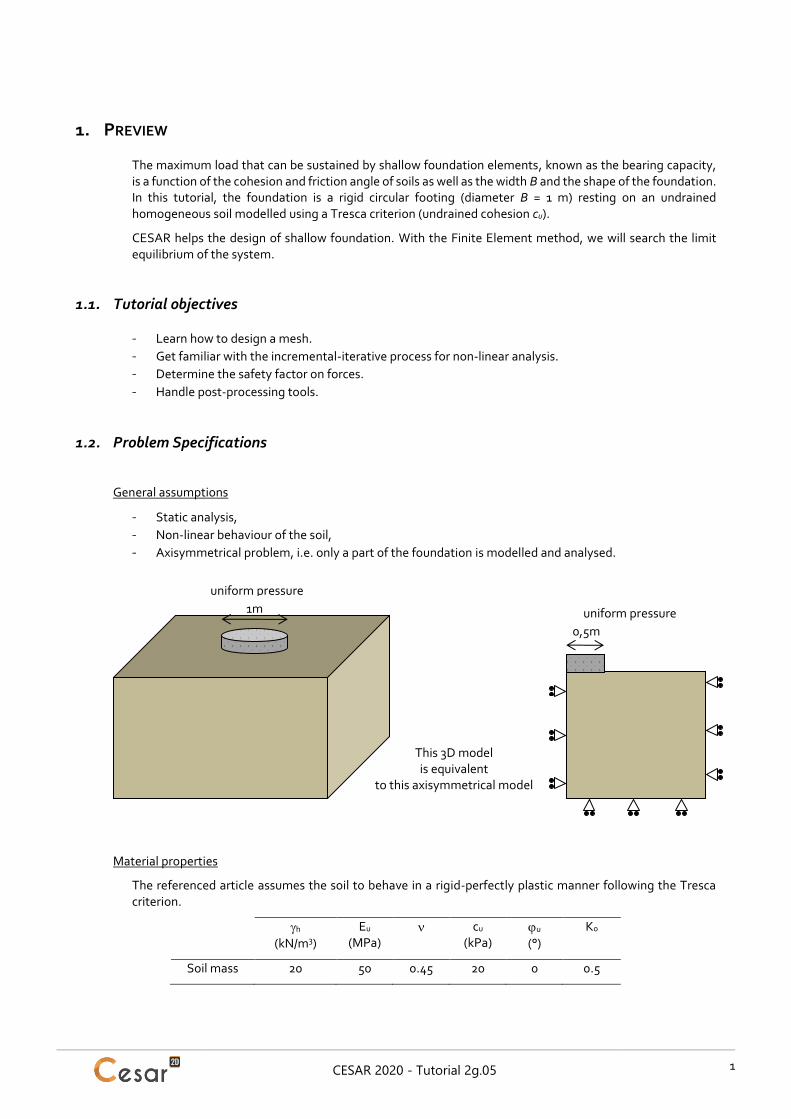
The maximum load that can be sustained by shallow foundation elements, known as the bearing capacity, is a function of the cohesion and friction angle of soils as well as the width B and the shape of the foundation. In this tutorial, the foundation is a rigid circular footing (diameter B = 1 m) resting on an undrained homogeneous soil modelled using a Tresca criterion (undrained cohesion cu).

CESAR helps the design of shallow foundation. With the Finite Element method, we will search the limit equilibrium of the system.

1.1. Tutorial objectives

- Learn how to design a mesh.

- Get familiar with the incremental-iterative process for non-linear analysis.

- Determine the safety factor on forces.

- Handle post-processing tools.

1.2. Problem Specifications

General assumptions

- Static analysis,

- Non-linear behaviour of the soil,

- Axisymmetrical problem, i.e. only a part of the foundation is modelled and analysed.

Material properties

The referenced article assumes the soil to behave in a rigid-perfectly plastic manner following the Tresca criterion.

h (kN/m3)

Eu (MPa)

cu (kPa)

u (°)

K0

Soil mass 20 50 0.45 20 0 0.5

This 3D model is equivalent

to this axisymmetrical model

uniform pressure

0,5m

1m

uniform pressure


2. GEOMETRY AND MESH

2.1. General settings

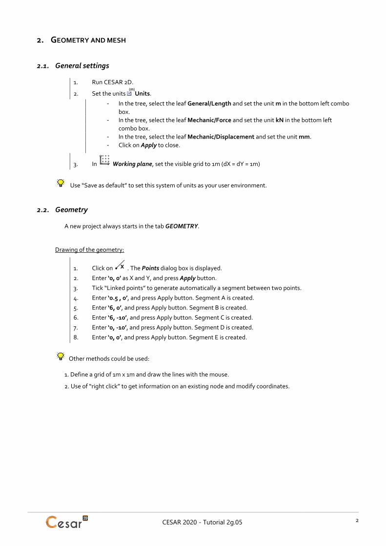
1. Run CESAR 2D.

2. Set the units Units.

- In the tree, select the leaf General/Length and set the unit m in the bottom left combo

box.

- In the tree, select the leaf Mechanic/Force and set the unit kN in the bottom left

combo box.

- In the tree, select the leaf Mechanic/Displacement and set the unit mm.

- Click on Apply to close.

3. In Working plane, set the visible grid to 1m (dX = dY = 1m)

Use “Save as default” to set this system of units as your user environment.

2.2. Geometry

A new project always starts in the tab GEOMETRY.

Drawing of the geometry:

1. Click on . The Points dialog box is displayed.

2. Enter ‘0, 0’ as X and Y, and press Apply button.

3. Tick “Linked points” to generate automatically a segment between two points.

4. Enter ‘0.5 , 0’, and press Apply button. Segment A is created.

5. Enter ‘6, 0’, and press Apply button. Segment B is created.

6. Enter ‘6, -10’, and press Apply button. Segment C is created.

7. Enter ‘0, -10’, and press Apply button. Segment D is created.

8. Enter ‘0, 0’, and press Apply button. Segment E is created.

Other methods could be used:

1. Define a grid of 1m x 1m and draw the lines with the mouse.

2. Use of “right click” to get information on an existing node and modify coordinates.


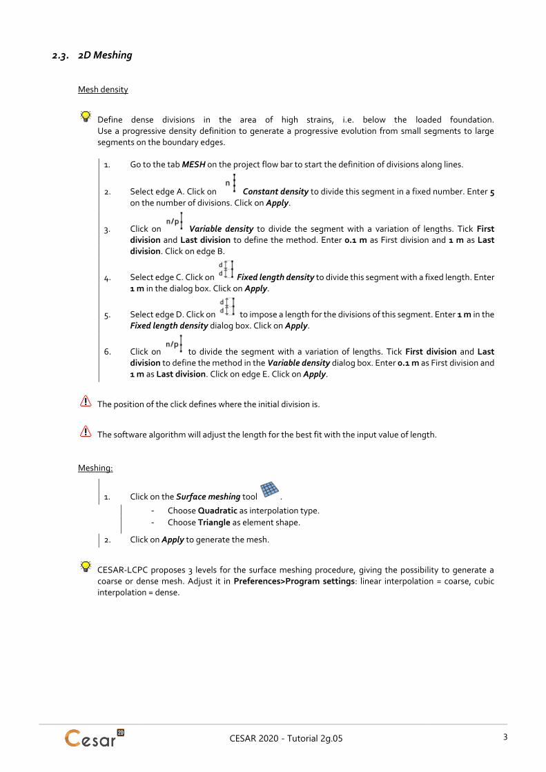
2.3. 2D Meshing

Mesh density

Define dense divisions in the area of high strains, i.e. below the loaded foundation. Use a progressive density definition to generate a progressive evolution from small segments to large segments on the boundary edges.

1. Go to the tab MESH on the project flow bar to start the definition of divisions along lines.

2. Select edge A. Click on Constant density to divide this segment in a fixed number. Enter 5 on the number of divisions. Click on Apply.

3. Click on Variable density to divide the segment with a variation of lengths. Tick First division and Last division to define the method. Enter 0.1 m as First division and 1 m as Last division. Click on edge B.

4. Select edge C. Click on Fixed length density to divide this segment with a fixed length. Enter 1 m in the dialog box. Click on Apply.

5. Select edge D. Click on to impose a length for the divisions of this segment. Enter 1 m in the Fixed length density dialog box. Click on Apply.

6. Click on to divide the segment with a variation of lengths. Tick First division and Last division to define the method in the Variable density dialog box. Enter 0.1 m as First division and 1 m as Last division. Click on edge E. Click on Apply.

The position of the click defines where the initial division is.

The software algorithm will adjust the length for the best fit with the input value of length.

Meshing:

1. Click on the Surface meshing tool .

- Choose Quadratic as interpolation type.

- Choose Triangle as element shape.

2. Click on Apply to generate the mesh.

CESAR-LCPC proposes 3 levels for the surface meshing procedure, giving the possibility to generate a coarse or dense mesh. Adjust it in Preferences>Program settings: linear interpolation = coarse, cubic interpolation = dense.


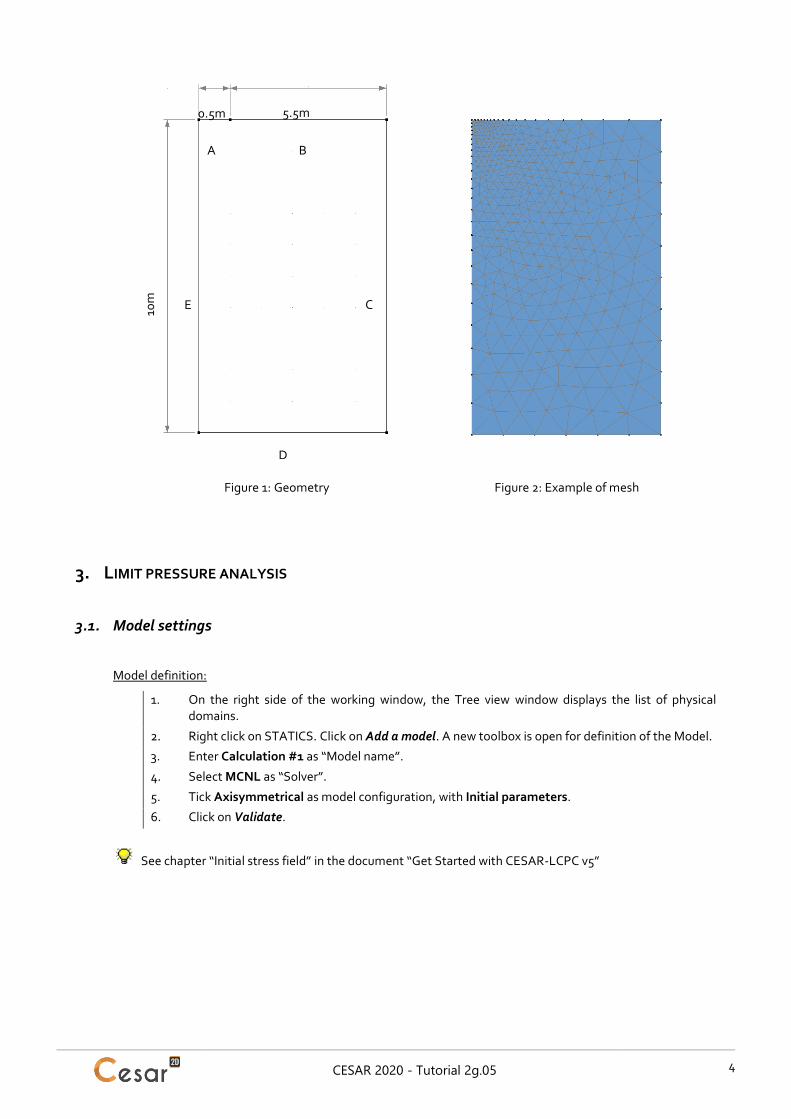
Figure 1: Geometry Figure 2: Example of mesh

3. LIMIT PRESSURE ANALYSIS

3.1. Model settings

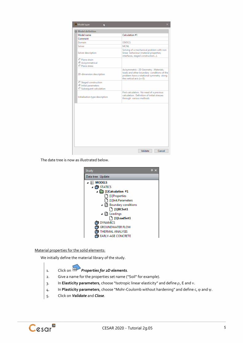
Model definition:

1. On the right side of the working window, the Tree view window displays the list of physical domains.

2. Right click on STATICS. Click on Add a model. A new toolbox is open for definition of the Model.

3. Enter Calculation #1 as “Model name”.

4. Select MCNL as “Solver”.

5. Tick Axisymmetrical as model configuration, with Initial parameters.

6. Click on Validate.

See chapter “Initial stress field” in the document “Get Started with CESAR-LCPC v5”

A B

C E

D

10m

5.5m 0.5m


The date tree is now as illustrated below.

Material properties for the solid elements:

We initially define the material library of the study.

1. Click on Properties for 2D elements.

2. Give a name for the properties set name (“Soil” for example).

3. In Elasticity parameters, choose “Isotropic linear elasticity” and define , E and .

4. In Plasticity parameters, choose “Mohr-Coulomb without hardening” and define c, and .

5. Click on Validate and Close.


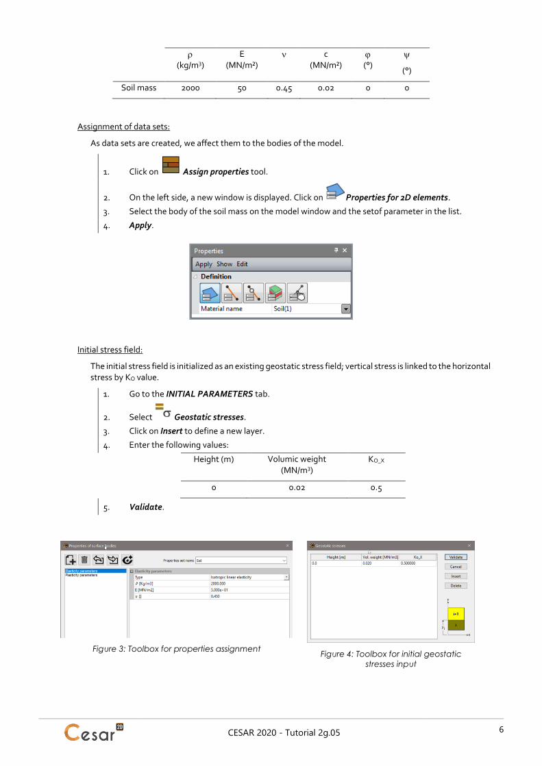
(kg/m3)

E (MN/m²)

c (MN/m²)

(°)

(°)

Soil mass 2000 50 0.45 0.02 0 0

Assignment of data sets:

As data sets are created, we affect them to the bodies of the model.

1. Click on Assign properties tool.

2. On the left side, a new window is displayed. Click on Properties for 2D elements.

3. Select the body of the soil mass on the model window and the setof parameter in the list.

4. Apply.

Initial stress field:

The initial stress field is initialized as an existing geostatic stress field; vertical stress is linked to the horizontal stress by KO value.

1. Go to the INITIAL PARAMETERS tab.

2. Select Geostatic stresses.

3. Click on Insert to define a new layer.

4. Enter the following values:

Height (m) Volumic weight (MN/m3)

KO_X

0 0.02 0.5

5. Validate.

Figure 3: Toolbox for properties assignment

Figure 4: Toolbox for initial geostatic

stresses input


Boundary conditions:

1. Go to the BOUNDARY CONDITIONS tab.

2. On the toolbar, activate to define side and bottom supports.

3. Apply. Supports are automatically affected to the limits of the mesh.

Default name of the boundary condition, BCSet1, set can be edited using the [F2] key.

Several boundary conditions sets are possible. Right click on Boundary conditions, in the data tree, to generate another one.

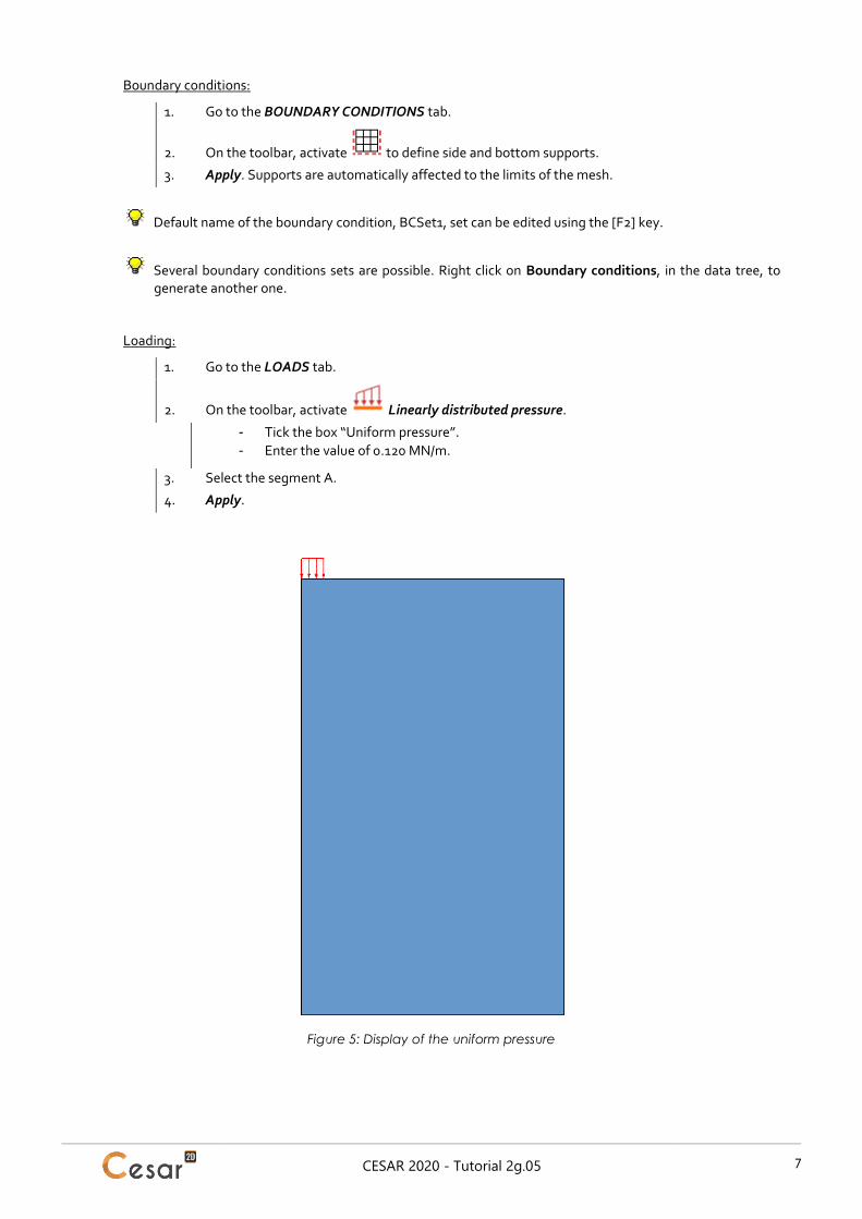
Loading:

1. Go to the LOADS tab.

2. On the toolbar, activate Linearly distributed pressure.

- Tick the box “Uniform pressure”.

- Enter the value of 0.120 MN/m.

3. Select the segment A.

4. Apply.

Figure 5: Display of the uniform pressure


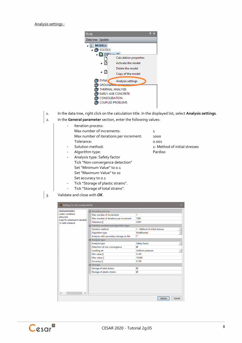
Analysis settings :

1. In the data tree, right click on the calculation title. In the displayed list, select Analysis settings.

2. In the General parameter section, enter the following values:

- Iteration process:

Max number of increments: 1

Max number of iterations per increment: 1000

Tolerance: 0.001

- Solution method: 1- Method of initial stresses

- Algorithm type: Pardiso

- Analysis type: Safety factor

Tick “Non-convergence detection”

Set “Minimum Value” to 0.1

Set “Maximum Value” to 10

Set accuracy to 0.1

- Tick “Storage of plastic strains”.

- Tick “Storage of total strains”.

3. Validate and close with OK.


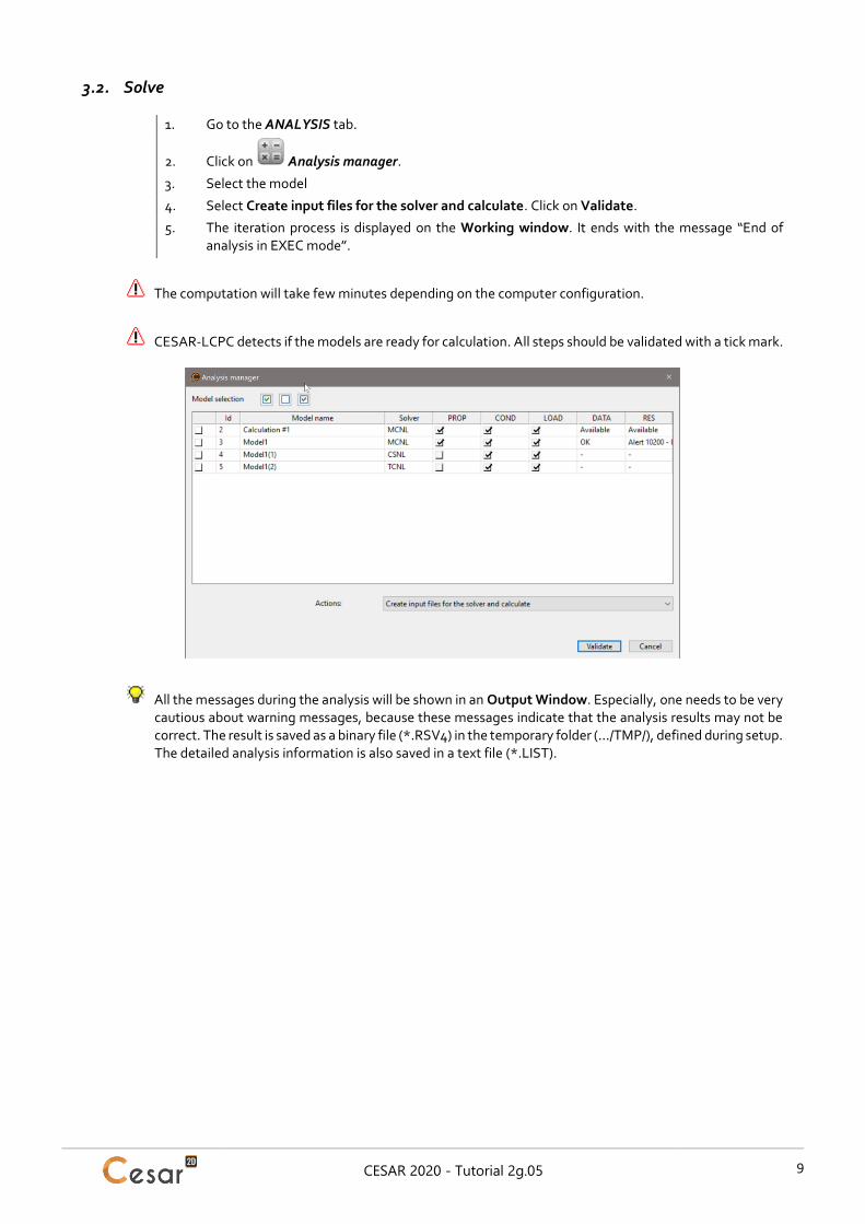
3.2. Solve

1. Go to the ANALYSIS tab.

2. Click on Analysis manager.

3. Select the model

4. Select Create input files for the solver and calculate. Click on Validate.

5. The iteration process is displayed on the Working window. It ends with the message “End of analysis in EXEC mode”.

The computation will take few minutes depending on the computer configuration.

CESAR-LCPC detects if the models are ready for calculation. All steps should be validated with a tick mark.

All the messages during the analysis will be shown in an Output Window. Especially, one needs to be very cautious about warning messages, because these messages indicate that the analysis results may not be correct. The result is saved as a binary file (*.RSV4) in the temporary folder (…/TMP/), defined during setup. The detailed analysis information is also saved in a text file (*.LIST).


3.3. Results

The result is the safety factor. It is displayed:

- In the Project window,

- In the listing file.

According to “Undrained bearing capacity factors for conical footings on clay”, G. T. Houlsby and C. M. Martin, Geotechnique 53, No. 5, 513–520, 2003; the ultimate bearing capacity obtained for the considered footing problem is:

p = 5.69 x cu = 113.8 kPa

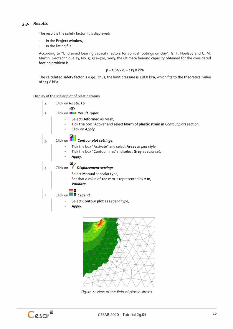
The calculated safety factor is 0.99. Thus, the limit pressure is 118.8 kPa, which fits to the theoretical value of 113.8 kPa.

Display of the scalar plot of plastic strains

1. Click on RESULTS

2. Click on Result Types

- Select Deformed as Mesh,

- Tick the box “Active” and select Norm of plastic strain in Contour plots section,

- Click on Apply.

3. Click on Contour plot settings.

- Tick the box “Activate” and select Areas as plot style,

- Tick the box “Contour lines”and select Grey as color set,

- Apply.

4. Click on Displacement settings.

- Select Manual as scalar type,

- Set that a value of 100 mm is represented by 2 m,

- Validate.

5. Click on Legend.

- Select Contour plot as Legend type,

- Apply.

Figure 6: View of the field of plastic strains


4. OTHER TYPES OF CALCULATIONS FOR DETERMINING THE LIMIT PRESSURE

4.1. Load controlled analysis

This analysis is similar to the previous one, with the difference that the process of loading is not automatic but user-defined.

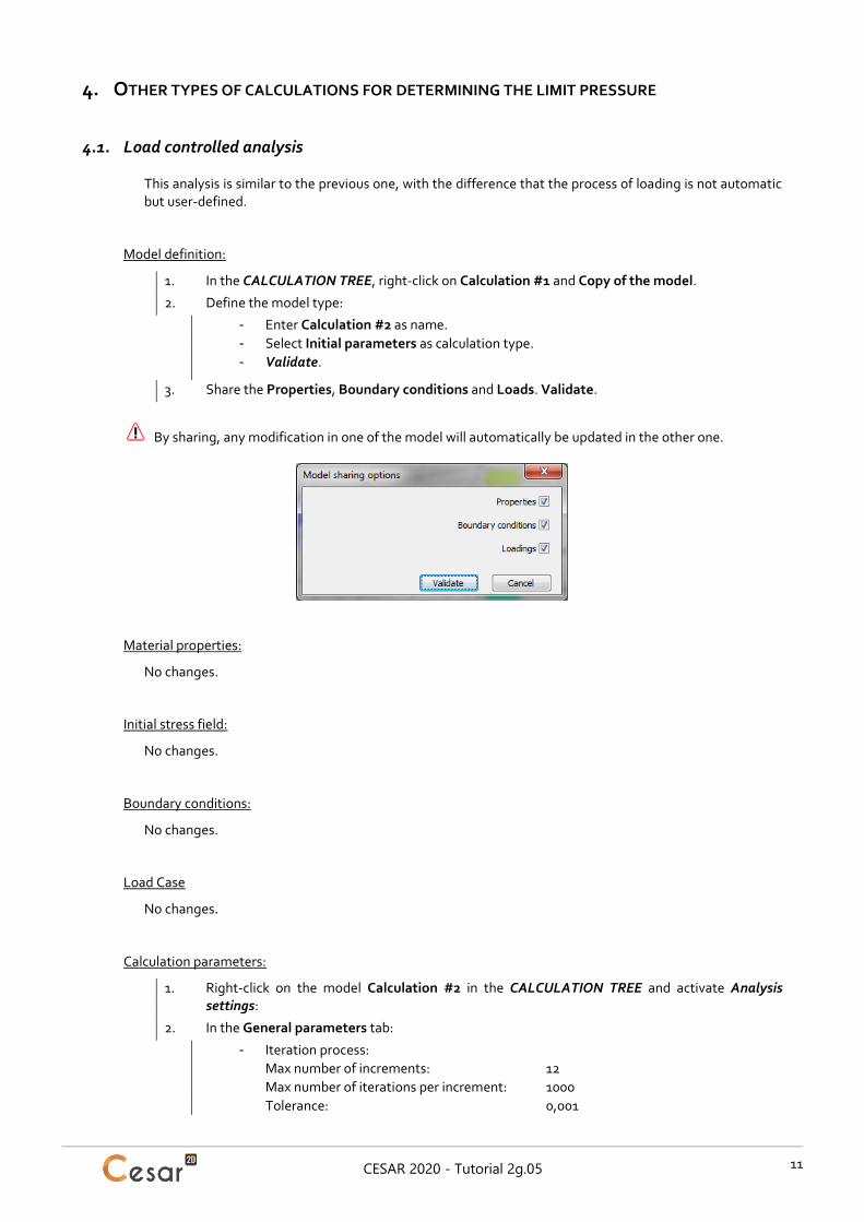
Model definition:

1. In the CALCULATION TREE, right-click on Calculation #1 and Copy of the model.

2. Define the model type:

- Enter Calculation #2 as name.

- Select Initial parameters as calculation type.

- Validate.

3. Share the Properties, Boundary conditions and Loads. Validate.

By sharing, any modification in one of the model will automatically be updated in the other one.

Material properties:

No changes.


No changes.


No changes.

Load Case

No changes.

Calculation parameters:

1. Right-click on the model Calculation #2 in the CALCULATION TREE and activate Analysis settings:

2. In the General parameters tab:




Tolerance: 0,001


- Solution method: 1- initial stresses

- Algorithm type: Pardiso

- Analysis type: Standard

3. Validate using OK.

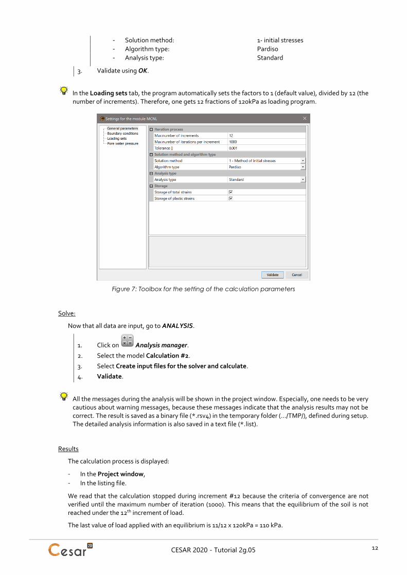
In the Loading sets tab, the program automatically sets the factors to 1 (default value), divided by 12 (the number of increments). Therefore, one gets 12 fractions of 120kPa as loading program.

Figure 7: Toolbox for the setting of the calculation parameters

Solve:

Now that all data are input, go to ANALYSIS.


2. Select the model Calculation #2.

3. Select Create input files for the solver and calculate.

4. Validate.

All the messages during the analysis will be shown in the project window. Especially, one needs to be very cautious about warning messages, because these messages indicate that the analysis results may not be correct. The result is saved as a binary file (*.rsv4) in the temporary folder (…/TMP/), defined during setup. The detailed analysis information is also saved in a text file (*.list).

Results

The calculation process is displayed:

- In the Project window,

- In the listing file.

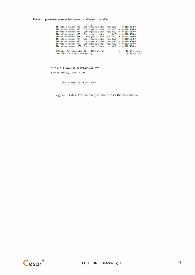
We read that the calculation stopped during increment #12 because the criteria of convergence are not verified until the maximum number of iteration (1000). This means that the equilibrium of the soil is not reached under the 12th increment of load.

The last value of load applied with an equilibrium is 11/12 x 120kPa = 110 kPa.


The limit pressure value is between 110 kPa and 120 kPa.

Figure 8: Extract of the listing at the end of the calculation


4.2. Displacement controlled analysis

This calculation is similar to the previous one. Only loads and boundary conditions are modified.

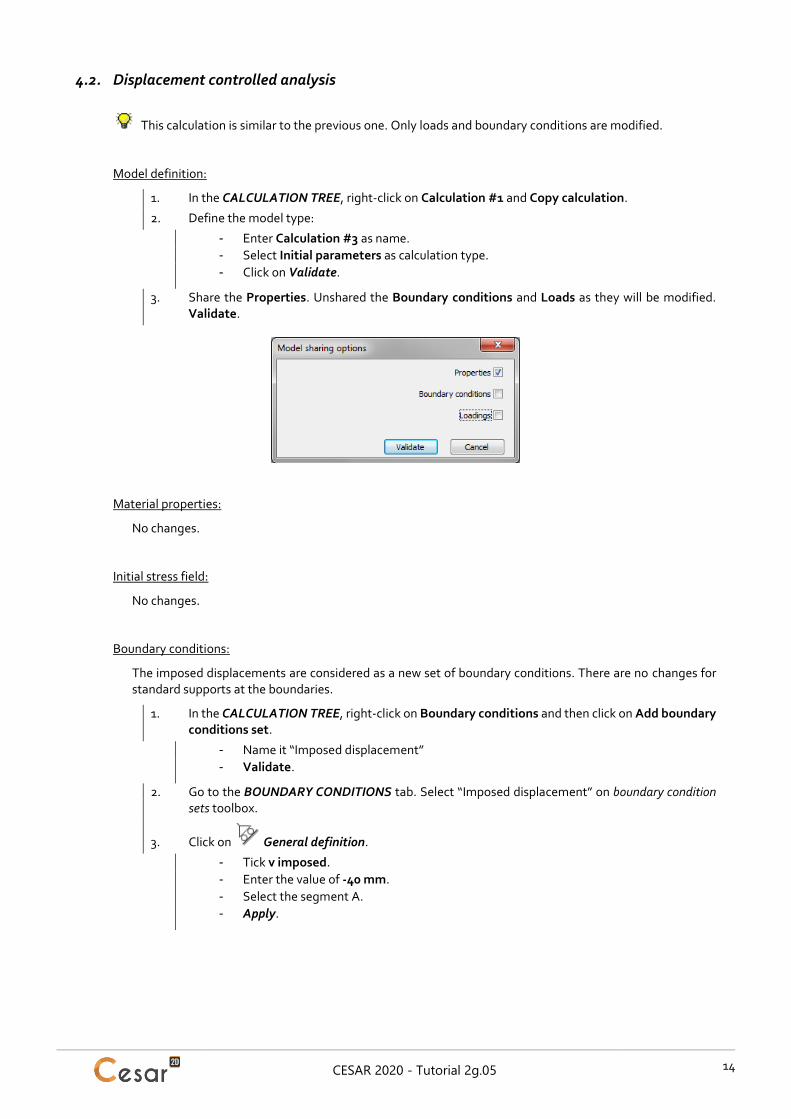
Model definition:

1. In the CALCULATION TREE, right-click on Calculation #1 and Copy calculation.

2. Define the model type:

- Enter Calculation #3 as name.

- Select Initial parameters as calculation type.

- Click on Validate.

3. Share the Properties. Unshared the Boundary conditions and Loads as they will be modified. Validate.

Material properties:

No changes.


No changes.


The imposed displacements are considered as a new set of boundary conditions. There are no changes for standard supports at the boundaries.

1. In the CALCULATION TREE, right-click on Boundary conditions and then click on Add boundary conditions set.

- Name it “Imposed displacement”

- Validate.

2. Go to the BOUNDARY CONDITIONS tab. Select “Imposed displacement” on boundary condition sets toolbox.

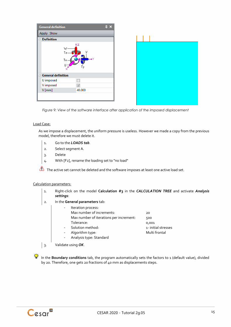
3. Click on General definition.

- Tick v imposed.

- Enter the value of -40 mm.

- Select the segment A.

- Apply.


Figure 9: View of the software interface after application of the imposed displacement

Load Case:

As we impose a displacement, the uniform pressure is useless. However we made a copy from the previous model, therefore we must delete it.

1. Go to the LOADS tab.

2. Select segment A.

3. Delete

4. With [F2], rename the loading set to "no load"

The active set cannot be deleted and the software imposes at least one active load set.

Calculation parameters:

1. Right-click on the model Calculation #3 in the CALCULATION TREE and activate Analysis settings:

2. In the General parameters tab:




Tolerance: 0,001

- Solution method: 1- initial stresses

- Algorithm type: Multi frontal

- Analysis type: Standard

3. Validate using OK.

In the Boundary conditions tab, the program automatically sets the factors to 1 (default value), divided by 20. Therefore, one gets 20 fractions of 40 mm as displacements steps.


Solve:

Now that all data are input, go to ANALYSIS.


2. Select the model Calculation #3.

3. Select Create input files for the solver and calculate. Click on Validate.


4.3. Alternative analyses

4.3.1 Linear elastic drained analysis with variable Young’s modulus

A non-linear elastic analysis can be carried out to assess the settlement under the footing in drained conditions. The increase of the modulus with depth is an important factor to take into consideration. Divide the model in several layers (2 m, 3 m and 5 m for example) and assess the drained modulus at the centre of each layer using the Ohde-Janbu empirical equation:

𝐸 = 𝐸𝑟𝑒𝑓 (𝜎𝑣

𝜎𝑟𝑒𝑓)

𝑁

with the following soil properties:

h (kN/m3)

E (MPa)

N

Soil mass 20 10

at ref = 100 kPa

0.7 0.33

4.3.2 Non-linear elastoplastic analysis with variable undrained cohesion

The increase of the undrained cohesion with depth is an important factor to take into consideration. Divide the upper part of the model in several thinner layers and assess the undrained cohesion at the centre of each layer using the following relationship:

𝜑𝑢 ≈ 0

𝑐𝑢 =1

2(𝜎′𝑣

𝑖𝑛𝑖 + 𝜎′ℎ𝑖𝑛𝑖) sin 𝜑 + 𝑐 cos 𝜑

with the following soil properties:

h (kN/m3)

Eu (MPa)

N cu (kPa)

u (°)

K0

Soil mass 20 50

at ref = 100 kPa

0.7 0.45 22 35 0.5

Note 1: The plasticity concentrating in the first meter of soil, the layers with varying cohesion must be thin enough to obtain the desired effect on the solution.

Note 2: Use the Ohde-Janbu formula to assess the undrained stiffness of each of the model layers.


4.4. Results

Load controlled analysis

The convergence is not achieved for the 12th step. This indicates that the soil is ruptured. The limit pressure value is between 110 kPa and 120 kPa.

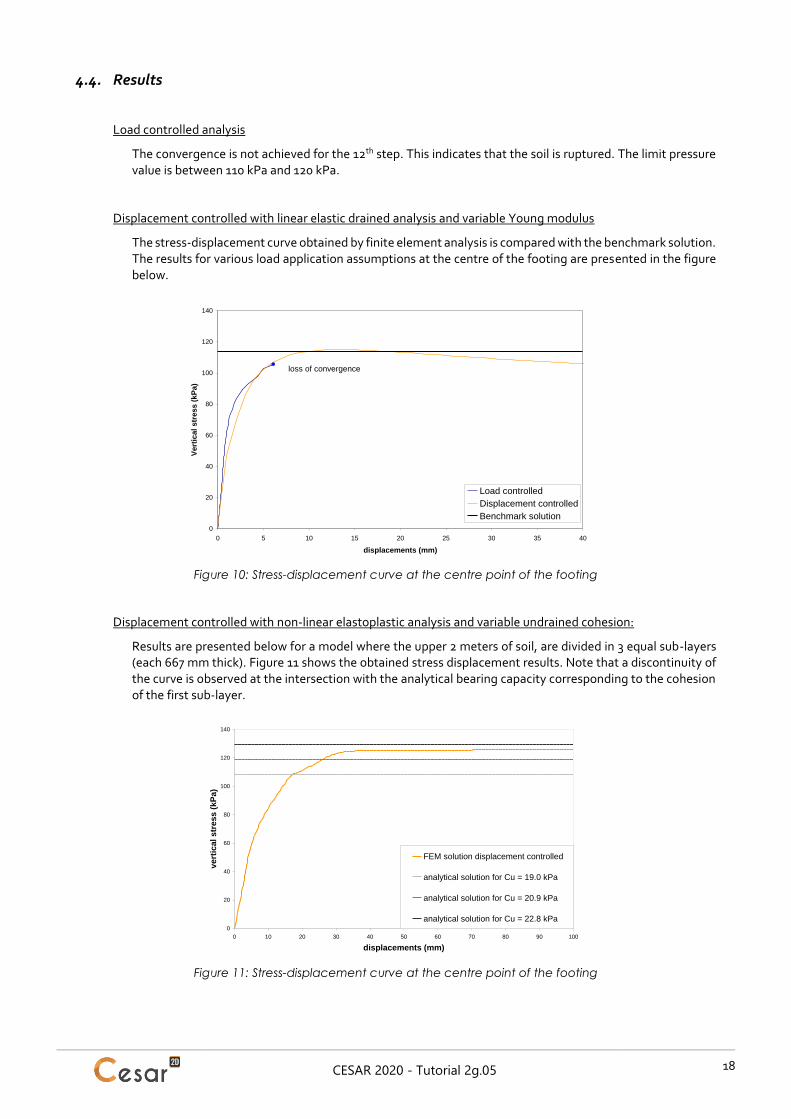
Displacement controlled with linear elastic drained analysis and variable Young modulus

The stress-displacement curve obtained by finite element analysis is compared with the benchmark solution. The results for various load application assumptions at the centre of the footing are presented in the figure below.

Figure 10: Stress-displacement curve at the centre point of the footing

Displacement controlled with non-linear elastoplastic analysis and variable undrained cohesion:

Results are presented below for a model where the upper 2 meters of soil, are divided in 3 equal sub-layers (each 667 mm thick). Figure 11 shows the obtained stress displacement results. Note that a discontinuity of the curve is observed at the intersection with the analytical bearing capacity corresponding to the cohesion of the first sub-layer.

Figure 11: Stress-displacement curve at the centre point of the footing

0

20

40

60

80

100

120

140

0 5 10 15 20 25 30 35 40

displacements (mm)

Ve

rtic

al

str

es

s (

kP

a)

Load controlled

Displacement controlled

Benchmark solution

loss of convergence

0

20

40

60

80

100

120

140

0 10 20 30 40 50 60 70 80 90 100

displacements (mm)

ve

rtic

al

str

es

s (

kP

a)

FEM solution displacement controlled

analytical solution for Cu = 19.0 kPa



Edited by :

8 quai Bir Hakeim

F-94410 SAINT-MAURICE

Tél. : +33 1 49 76 12 59

[email protected]

www.cesar-lcpc.com

© itech - 2020

Documents

CESAR 2D - Tutorial 2g.05 - Bearing capacity of a shallow