CERA - BOEM Homepage | BOEM · 2019-10-14 · OCS Study BOEM 2011-xxx IHS CERA Comparative Assessment of the Federal Oil and Gas Fiscal System Final Report Author Irena Agalliu October

OCS Study BOEM 2011-xxx

Comparative Assessment of the Federal Oil and Gas Fiscal System Final Report

U.S. Department of the Interior Bureau of Ocean Energy Management

U.S. Department of the Interior Bureau of Land Management

CERA

OCS Study BOEM 2011-xxx

IHS CERA

Comparative Assessment of the Federal Oil and Gas Fiscal System Final Report

Author

Irena Agalliu

October 2011 Prepared under BOEM Contract M10PC00090 IHS Cambridge Energy Research Associates 55 Cambridge Parkway Cambridge, Massachusetts, 02142

Published by:

U.S. Department of the Interior Bureau of Ocean Energy Management

U.S. Department of the Interior Bureau of Land Management

iii

DISCLAIMER

This report was prepared under contract between the U.S. Department of the Interior, Bureau of Ocean Energy Management, Regulation and Enforcement and Bureau of Land Management and IHS Cambridge Energy Research Associates. The opinions, conclusions, or recommendations expressed in it do not necessarily reflect the view and policies of BOEM and BLM, nor does mention of trade names or commercial products constitute endorsement or recommendation for use.

REPORT AVAILABILITY

Extra copies of the report may be obtained from the Public Information Office (Mail Stop 5034) at the following address:

U.S. Department of the Interior

Bureau of Ocean Energy Management

381 Elden Street

Herndon VA 20170

CITATION

Suggested citation:

Agalliu, I. 2011. Comparative assessment of the federal oil and gas fiscal systems. U.S. Department of the Interior, Bureau of Ocean Energy Management Herndon. VA. OCS Study, BOEM 2011-xxx. 300 pp.

ACKNOWLEDGMENTS

Thanks are extended to David Hobbs who advised on this project, the expert reviewers Emil Sunley and Carole Nakhle, and the Department of Interior team led by Dr. Radford Schantz for their helpful suggestions and comments. The author would like to acknowledge Rick Chamberlain, Tim Zoba, Curtis Smith, Aube Plop Montero, Diane Betts, Gina Hsieh, Imre Kugler, Shawn Gallagher, Adebola Adejumo, Taner Sensoy, Horacio Cuenca, and Jim Watkins, for the cooperation, encouragement , support and the tremendous effort in collecting information and developing the cost and economic models for this study.

iv

ABSTRACT

The competitiveness of oil and gas fiscal systems is often based on random ranking of jurisdictions without taking into consideration the relative prospectivity of the respective jurisdiction, the varying policy objectives, and socioeconomic drivers, not to mention the different investment environments, distance from markets, commodity prices, typical finding and development cost, relative size of discoveries, well productivity, and other factors. Analyses that focus solely on government take fail to account for the limitations of the government take statistic. A composite index that compares fiscal systems on government take as well as measures of profitability, revenue risk, and fiscal stability in relation to the relative prospectivity and policy objectives is a more objective and thorough approach to comparing fiscal systems. This report compares the oil and gas federal fiscal systems against a selected peer group of jurisdictions that compete for investment in the upstream oil and gas industry.

v

TABLE OF CONTENTS

ABSTRACT ................................................................................................................................ iv

TABLE OF CONTENTS................................................................................................................ v

LIST OF FIGURES ...................................................................................................................... ix

LIST OF TABLES ....................................................................................................................... xii ABBREVIATIONS, ACRONYMS AND SYMBOLS ..................................................................... xvii EXECUTIVE SUMMARY ............................................................................................................ 1

1. Introduction ................................................................................................................ 1

2. Objective of the Study ................................................................................................ 2

3. About IHS CERA ........................................................................................................... 2

4. Approach ..................................................................................................................... 2

4.1 Finding the Right Peer Group.............................................................................. 3

5. Government Take on Federal Lands ........................................................................... 5

6. Fair Share .................................................................................................................... 6

6.1 What Is Fair Share? ............................................................................................. 7

7. Resource Endowment ............................................................................................... 10

8. Ranking of Fiscal Systems ......................................................................................... 11

8.1 Ranking of Fiscal Terms ..................................................................................... 13

8.2 Revenue Risk ..................................................................................................... 15

8.2.1 Revenue Risk Index....................................................................................... 18

8.3. Fiscal Stability .................................................................................................... 20

8.4 Composite Index ............................................................................................... 22

9. Alternative Fiscal Systems......................................................................................... 24

10. Conclusion ............................................................................................................. 28

1. CONTEXT AND SCOPE ................................................................................................... 31

1.1 Approach ............................................................................................................... 31

1.1.1 Size and Availability of the Oil and Gas Resources in Place .......................... 32

1.1.2 Finding and Development Costs ................................................................... 32

1.1.3 Price and Cost Scenarios ............................................................................... 33

1.1.4 Finding the Right Peer Group........................................................................ 36

1.1.4.1 Worldwide Approach ............................................................................ 36

1.1.4.2 Regional Comparisons .......................................................................... 36

1.1.4.3 Similar Cost Environments .................................................................... 36

1.1.4.4 IHS CERA Fiscal System Selection Criteria ............................................ 37

1.1.5 Ranking of Fiscal Systems ............................................................................. 41

1.2 Organization of the Report ................................................................................... 43

2. DESIGN OF PETROLEUM FISCAL SYSTEMS .................................................................... 45

2.1 Overview ............................................................................................................... 45

2.2 The Concept of Government Take ........................................................................ 47

2.2.1 Definition and Use of Government Take ...................................................... 47

2.2.2. Components of Government Take................................................................ 48

2.2.2.1 Ad Valorem, or Production-Based Levies ............................................ 48

vi

2.2.2.2 Profit-based Levies ................................................................................ 50

2.2.2.3 Equity Participation ............................................................................... 52

2.2.2.4 Quasi-fiscal Instruments ........................................................................ 54

2.2.3 Limitations of Government Take .................................................................. 55

2.3 Literature Review .................................................................................................. 56

2.3.1 Government Take Referenced by GAO ......................................................... 56

2.3.2 The Government Take for New Acreage ...................................................... 60

2.3.3 Fair Share ...................................................................................................... 63

2.3.4 What Is Fair Share? ....................................................................................... 65

2.4 Features of U.S. Federal Oil and Gas Fiscal Systems............................................. 69

3. FACTORS INFLUENCING GOVERNMENT TAKE AND INVESTMENT DECISIONS ............. 71

3.1 Resource Endowment ........................................................................................... 71

3.2 Political and Commercial Risk ............................................................................... 74

3.3 Policy Goals and Constraints ................................................................................. 77

3.3.1 Value Added Through Expeditious and Orderly Development .................... 78

3.3.2 Restricting Access ......................................................................................... 81

3.3.3 Mixed Approaches ........................................................................................ 82

3.3.4 New Markets ................................................................................................. 83

3.3.5 Evolving Energy Policies and the Environment ............................................. 83

4. RANKING BY GOVERNMENT TAKE AND OTHER INDICATORS ....................................... 84

4.1 Approach ............................................................................................................... 84

4.2 Government Take and Profitability Indicators ..................................................... 85

4.2.1 Offshore Fiscal Systems ................................................................................ 85

4.2.2 North American Fiscal Systems ..................................................................... 91

4.3 Fiscal System Flexibility ......................................................................................... 94

4.4 Fiscal Terms Index ................................................................................................. 98

5. REVENUE RISK DISTRIBUTION ..................................................................................... 103

5.1 Sources of Risk ..................................................................................................... 103

5.2 Risk-Reward Structure of Federal Fiscal Systems ............................................... 107

5.2.1 Bonus Bids ................................................................................................... 107

5.2.2 Royalty ......................................................................................................... 108

5.2.3 Income Tax .................................................................................................. 109

5.3 Revenue Risk Ranking ......................................................................................... 111

6. FISCAL STABILITY ......................................................................................................... 114

6.1 Stability Index Variables ...................................................................................... 116

6.1.1 Type of Change ........................................................................................... 116

6.1.2 Applicability of Change ............................................................................... 118

6.1.3 Degree of Change ........................................................................................ 119

6.1.4 Frequency of Change ................................................................................. 121

6.2 Market Reaction to Changes in Fiscal Terms—Case Studies .............................. 124

6.2.1 The Case of Alaska ....................................................................................... 125

6.2.2 Alberta—Tracing Back Its Steps .................................................................. 126

7. COMPOSITE INDEX ...................................................................................................... 128

8. APPLICATION OF ALTERNATIVE FISCAL SYSTEMS ....................................................... 132

vii

8.1 Alternative Royalty Rates .................................................................................... 132

8.2 Comparative Analysis of Alternative Royalty Rates ............................................ 132

8.2.1 Royalty Alternatives in Gulf of Mexico ....................................................... 132

8.2.2 Royalty Alternatives in Wyoming ................................................................ 137

8.3 Break-even Prices ................................................................................................ 143

8.4 Final Ranking ....................................................................................................... 147

9. RECOMMENDATION FOR FUTURE UPDATES .............................................................. 148

10. CONCLUSION .............................................................................................................. 149

BIBLIOGRAPHY .................................................................................................................... 151

APPENDIX I—FIELD SELECTION CRITERIA ........................................................................... 155

1. Selection of Fields on Federal Lands ............................................................... 159

2. Selection of Fields in Other Jurisdictions ........................................................ 163

APPENDIX II—ASSUMED FISCAL TERMS ............................................................................. 177

A. Model Assumptions ................................................................................................ 177

B. Fiscal Systems ......................................................................................................... 178

1. ALGERIA ONSHORE ......................................................................................... 178

2. ANGOLA—OFFSHORE ..................................................................................... 180

3. AUSTRALIA—OFFSHORE FEDERAL JURISDICTION .......................................... 182

4. AUSTRALIA—QUEENSLAND COALBED GAS .................................................... 183

5. BRAZIL—DEEPWATER ..................................................................................... 184

6. CANADA—ALBERTA CONVENTIONAL OIL ...................................................... 189

7. CANADA—ALBERTA OIL SANDS...................................................................... 193

8. CANADA—BRITISH COLUMBIA SHALE GAS .................................................... 195

9. CHINA—OFFSHORE ........................................................................................ 197

10. COLOMBIA—ONSHORE................................................................................... 200

11. GERMANY—ONSHORE .................................................................................... 203

12. INDIA—DEEPWATER ....................................................................................... 204

13. INDONESIA—OFFSHORE CONVENTIONAL GAS .............................................. 206

14. INDONESIA—ONSHORE COALBED GAS .......................................................... 208

15. KAZAKHSTAN—OFFSHORE .............................................................................. 209

16. LIBYA—ONSHORE ........................................................................................... 213

17. MALAYSIA—OFFSHORE ................................................................................... 215

18. NORWAY—OFFSHORE .................................................................................... 218

19. POLAND—ONSHORE GAS ............................................................................... 219

20. RUSSIA—ONSHORE ......................................................................................... 220

21. UNITED KINGDOM—OFFSHORE ..................................................................... 223

22. UNITED STATES—ALASKA: STATE LANDS ....................................................... 225

23. UNITED STATES—LOUISIANA: STATE LANDS .................................................. 230

24. UNITED STATES—TEXAS: STATE LANDS .......................................................... 232

25. UNITED STATES—OUTER CONTINENTAL SHELF: DEEPWATER GULF OF MEXICO ………………………………………………………………………………………………………………….. 234

26. UNITED STATES—OUTER CONTINENTAL SHELF—GULF OF MEXICO SHELF ... 236

27. UNITED STATES—FEDERAL LANDS: WYOMING .............................................. 237

28. VENEZUELA—NON-ASSOCIATED GAS TERMS ................................................ 239

viii

29. VENEZUELA—HEAVY OIL TERMS .................................................................... 241

APPENDIX III—RESULTS OF ECONOMIC ANALYSIS ............................................................. 243

1. AVERAGE GOVERNMENT TAKE, PI, AND IRR INDICATORS ................................. 250

2. INDIVIDUAL FIELD RESULTS AND AVERAGE INDICATORS PER FISCAL SYSTEM .. 254

3. INDIVIDUAL FIELD RESULTS AND AVERAGE INDICATORS FOR ALTERNATIVE ROYALTIES ON FEDERAL LANDS .......................................................................... 265

APPENDIX IV—CHANGES IN FISCAL TERMS OVER THE PAST FIVE YEARS .......................... 272

APPENDIX V—INDEX TABLES .............................................................................................. 283

ix

LIST OF FIGURES Figure 1: Government Action Reflecting Commodity Prices .......................................................... 1

Figure 2: Government Take Variance in Five Coalbed Gas Fields ................................................... 6

Figure 3: DOI OCS Revenue (Fiscal Year 2005–2010) ..................................................................... 8

Figure 4: DOI Wyoming Revenue (Fiscal Year 2006–2010) ............................................................ 9

Figure 5: Government Take Relative to Remaining Recoverable Reserve Ranking ..................... 11

Figure 6: Fiscal Terms Index—Offshore ........................................................................................ 13

Figure 7: Fiscal Terms Index—Onshore North America................................................................ 14

Figure 8: Fiscal Terms Index .......................................................................................................... 15

Figure 9: Revenue Risk Ranking—Onshore North America .......................................................... 18

Figure 10: Revenue Risk Ranking—Worldwide Onshore .............................................................. 19

Figure 11: Revenue Risk Ranking Worldwide Offshore ................................................................ 20

Figure 12: Fiscal Stability Index ..................................................................................................... 21

Figure 13: Composite Index—Ranking of Offshore Systems ........................................................ 22

Figure 14: Composite Index—Ranking of Onshore North American Fiscal Systems .................... 23

Figure 15: Composite Index—Global Rating and Ranking ............................................................ 24

Figure 16: Average Bid per Acre Onshore North America ............................................................ 27

Figure 17: Composite Index: Alternative Fiscal Systems—Global Ranking .................................. 28

Figure 1.1: Crude Oil and Upstream Capital Costs Indexes .......................................................... 35

Figure 1.2: Composite Index Variables ......................................................................................... 43

Figure 2.1.a: Government Take for a Low-Cost Project ................................................................ 58

Figure 2.1.b: Government Take for a High-Cost Project ............................................................... 59

Figure 2.2.a: DOI OCS Revenue (Fiscal Years 2005–2010) ............................................................ 67

Figure 2.2.b: GOM Bonus Payments (Fiscal Years 2005–2010) .................................................... 68

Figure 2.3: DOI Wyoming Revenue (Fiscal Years 2006–2010) ...................................................... 68

Figure 3.1: E&P Activity Scorecard ................................................................................................ 72

Figure 3.2: Field Sizes per New-field Wildcats .............................................................................. 73

Figure 3.3: Government Take Relative to Remaining Recoverable Reserve Ranking .................. 74

Figure 3.4: Adverse Changes in Fiscal Terms (2005–2010) .......................................................... 76

Figure 3.5: Net Oil Imports and Exports, 2009 ............................................................................. 78

Figure 4.1.a: Undiscounted Cash Flow Components of Seven Gulf of Mexico Shelf Natural Gas Fields ............................................................................................................................................. 87

Figure 4.1.b: Undiscounted Cash Flow Components of Three Gulf of Mexico Shelf Oil Fields .... 87

Figure 4.2.a: Undiscounted Cash Flow Components of Five Gulf of Mexico Deepwater Gas Fields....................................................................................................................................................... 88

Figure 4.2.b: Undiscounted Cash Flow Components of Five Gulf of Mexico Deepwater Oil Fields....................................................................................................................................................... 89

Figure 4.3.a: Percentage of Average Government Take—Offshore Fiscal Systems ..................... 90

Figure 4.3.b: Average PI—Offshore Fiscal Systems ...................................................................... 90

Figure 4.3.c: Average IRR—Offshore Fiscal Systems .................................................................... 91

Figure 4.4: Undiscounted Cash Flow Components of Five Wyoming Conventional Gas Fields ... 92

Figure 4.5: Undiscounted Cash Flow Components of Five Wyoming Coalbed Gas Fields ........... 93

x

Figure 4.6: Comparison of North American Onshore Fiscal Systems—Government Take and Profitability Indicators .................................................................................................................. 95

Figure 4.7: Rigid Price Thresholds Adopted by Select Countries .................................................. 96

Figure 4.8: Degree of Change in Government Take with 20 Percent Increase in IRR .................. 97

Figure 4.9: Progressivity/Regressivity Index ................................................................................. 98

Figure 4.10: Fiscal Terms Index—Offshore ................................................................................... 99

Figure 4.11: Fiscal Terms Index—Onshore North America ........................................................ 100

Figure 4.12: Comparison of Federal Fiscal Systems—Government Take and Profitability Indicators .................................................................................................................................... 101

Figure 4.13: Fiscal Terms Index ................................................................................................... 102

Figure 5.1: Alberta and British Columbia Average Bonus per Hectare ....................................... 108

Figure 5.2: Share of Total Government Revenue at One-quarter of Producing Field Life (discounted at 10 percent) ......................................................................................................... 111

Figure 5.3: Revenue Risk Ranking—Onshore North America ..................................................... 112

Figure 5.4: Revenue Risk Ranking—Worldwide Onshore ........................................................... 113

Figure 5.5: Revenue Risk Ranking—Worldwide Offshore .......................................................... 113

Figure 6.1: Increase of Government Take (2005–2011) ............................................................. 116

Figure 6.2: Fiscal Stability Index—Worldwide Offshore ............................................................. 122

Figure 6.3: Fiscal Stability Index—Onshore North America ....................................................... 123

Figure 6.4: Fiscal Stability Index .................................................................................................. 124

Figure 6.4: Alaska—Acreage Awarded (2005–2010) .................................................................. 126

Figure 6.5: Percentage of Land Sales in Western Canadian Provinces ....................................... 127

Figure 6.6: Alberta Oil Sands—Acreage Awarded (2005–2010) ................................................. 127

Figure 7.1: Composite Index—Ranking of Offshore Fiscal Systems ........................................... 129

Figure 7.2: Composite Index—Ranking of Onshore North American Fiscal Systems ................. 130

Figure 7.3: Composite Index—Global Rating and Ranking ......................................................... 131

Figure 8.1: Fiscal Terms Index Offshore—Alternative Royalty Rates ......................................... 134

Figure 8.2: Offshore Revenue Risk—Alternative Royalty Comparison ....................................... 135

Figure 8.3: Fiscal System Stability—Alternative Offshore Systems ............................................ 136

Figure 8.4: Composite Index: Alternative Fiscal Systems—Offshore Comparison ..................... 137

Figure 8.5: Fiscal Terms Index: North American Comparison of Alternative Fiscal Systems ..... 139

Figure 8.6: Average Bid per Acre Onshore North America ......................................................... 140

Figure 8.7: Revenue Risk Score for North American Jurisdictions—Alternative Royalty Comparison ................................................................................................................................. 141

Figure 8.8: Fiscal System Stability–Alternative North American Systems .................................. 142

Figure 8.9: Composite Index: Alternative Fiscal Systems—Onshore North American Comparison..................................................................................................................................................... 143

Figure 8.10: Gulf of Mexico Natural Gas Break-even Prices at 10 Percent IRR .......................... 144

Figure 8.11: Gulf of Mexico Natural Gas Break-even Prices at 15 Percent IRR .......................... 144

Figure 8.12: Gulf of Mexico Crude Oil Break-even Prices at 10 Percent IRR .............................. 145

Figure 8.13: Gulf of Mexico Crude Oil Break-even Prices at 15 Percent IRR .............................. 145

Figure 8.14: Wyoming Natural Gas Break-even Prices at 10 Percent IRR .................................. 146

Figure 8.15: Wyoming Natural Gas Break-even Prices at 15 Percent IRR .................................. 146

Figure 8.16: Composite Index: Alternative Fiscal Systems—Global Ranking ............................. 147

xi

Figure I-I: Selected Fields ............................................................................................................ 156

Figure I-II: Gulf of Mexico Proved Gas Reserves ......................................................................... 159

Figure I-III: Gulf of Mexico Proved Oil Reserves ......................................................................... 160

Figure I-IV: Gulf of Mexico Shelf Discovered Fields (2000–2010) ............................................... 160

Figure I-V: Gulf of Mexico Deepwater Field Discoveries (2000–2010) ....................................... 161

Figure I-VI: Wyoming Federal Lands Fields Discovered (2000–2010) ........................................ 162

Figure I-VII: Algeria Onshore Discoveries (2000–2010) .............................................................. 163

Figure I-VIII: Angola Offshore Discoveries (2000–2010) ............................................................. 164

Figure I-IX: Australia Offshore Discoveries (2000–2010) ............................................................ 164

Figure I-X: Brazil Offshore Discoveries (2000–2010) .................................................................. 165

Figure I-XI: Canada (Alberta) Discoveries (2000–2010) .............................................................. 166

Figure I-XII: China Offshore Discoveries (2000–2010) ................................................................ 167

Figure I-XIII: Colombia Onshore Discoveries (2000–2010) ......................................................... 167

Figure I-XIV: India Offshore Discoveries (2000–2010) ................................................................ 168

Figure I-XV: Indonesia Offshore Discoveries (2000–2010) ......................................................... 169

Figure I-XVI: Kazakhstan Offshore Discoveries (2000–2010) ...................................................... 170

Figure I-XVII: Libya Onshore Discoveries (2000–2010) ............................................................... 170

Figure I-XVIII: Malaysia Offshore Discoveries (2000–2010) ....................................................... 171

Figure I-XIX: Norway Discoveries (2000–2010) ........................................................................... 171

Figure I-XX: Poland Conventional Field Discoveries (2000–2010) .............................................. 172

Figure I-XXI: Russia Onshore Discoveries (2000–2010) .............................................................. 173

Figure I-XXII: United Kingdom Offshore Discoveries (2000–2010) ............................................. 173

Figure I-XXIII: U.S. Louisiana Onshore Discoveries on State Land (2000–2010) ......................... 174

Figure I-XXIV: U.S. Texas Onshore Discoveries on State Land (2000–2010) ............................... 175

Figure I-XXV: Venezuela Onshore Discoveries (2000–2010) ...................................................... 175

xii

LIST OF TABLES Table 1: 29 Fiscal Systems Selected for Study ................................................................................ 4

Table 2: Composite Index ............................................................................................................. 12

Table 3: Revenue Risk of Fiscal Instruments ................................................................................. 16

Table 4: Fiscal Stability Index Weights .......................................................................................... 21

Table 5: Alternative Sliding Scale Royalty Rates ........................................................................... 25

Table 6: Average Indicators for Alternative Royalty Rates in the Gulf of Mexico ........................ 25

Table 1.1: E&P Rating and Ranking Approach .............................................................................. 39

Table 1.2: 29 Fiscal Systems Selected for Study ........................................................................... 41

Table 2.1: Royalty and Severance Tax Rates ................................................................................. 49

Table 2.2: Range of Income Tax Rates .......................................................................................... 50

Table 2.3: Range of Special Petroleum Taxes ............................................................................... 51

Table 2.4: Production Sharing Mechanisms ................................................................................. 52

Table 2.5: State Participation ........................................................................................................ 53

Table 2.6: Bonus Types ................................................................................................................. 54

Table 2.7: Studies Referenced by GAO ......................................................................................... 57

Table 2.8: Reliance on Profit-Based Levies ................................................................................... 62

Table 2.9: Impact of Royalty Alternatives on Exploration and Production Activity in the Gulf of Mexico ........................................................................................................................................... 64

Table 2.10: Impact of Royalty Alternatives on Federal Government Revenue from the Gulf of Mexico ........................................................................................................................................... 64

Table 2.11: Gulf of Mexico Federal Fiscal Systems ....................................................................... 69

Table 2.12: Wyoming Federal Fiscal System ................................................................................. 70

Table 3.1: Oil Revenue Share of GDP of Major OECD Countries .................................................. 80

Table 3.2: Oil Revenue Share of GDP of North American Jurisdictions ........................................ 80

Table 3.3: Impact of Oil and Gas Activities on Employment, Labor Income, and Value Added in Four U.S. States ............................................................................................................................. 81

Table 3.4: Oil Revenue Share of GDP of Major Exporting Countries ............................................ 81

Table 5.1 Revenue Risk—Fiscal Instruments .............................................................................. 104

Table 5.2: Fiscal System Components ......................................................................................... 105

Table 5.3: Average Bonus Bids per Acre ..................................................................................... 108

Table 5.4: Shift in Licensing Activities (2008–2009) ................................................................... 110

Table 6.1: Type of Change Category—Fiscal Stability Index ....................................................... 117

Table 6.2: Stability Ranking—Type of Change ............................................................................ 117

Table 6.3: Applicability of Change Category—Fiscal Stability Index ........................................... 118

Table 6.4: Stability Ranking—Applicability of Change ................................................................ 119

Table 6.5: Stability Ranking—Degree of Change ........................................................................ 120

Table 6.6: Stability Ranking—Frequency of Change ................................................................... 121

Table 6.7: Fiscal Stability Index Methodology ............................................................................ 122

Table 7.1: Composite Index ........................................................................................................ 129

Table 8.1: Alternative Sliding Scale Royalty Rates ...................................................................... 132

Table 8.2: Average Indicators for Alternative Royalty Rates in Gulf of Mexico ......................... 133

Table: 8.3: Average Indicators for Alternative Royalty Rates on Wyoming Federal Lands ........ 138

xiii

Table I-I: Fiscal Systems and Resource Type ............................................................................... 157

Table I-II: U.S. Wyoming Coalbed Gas Projects........................................................................... 163

Table I-III: Australia (Queensland) Coalbed Gas Fields Modeled ............................................... 165

Table I-IV: Canada (Alberta) Oil Sands Modeled ........................................................................ 166

Table I-V: Canada (British Columbia) Shale and Tight Gas Plays Modeled ................................. 166

Table I-VI: Germany Shale Gas Models ....................................................................................... 168

Table I-VII: Indonesia Coalbed Gas Fields Modeled .................................................................... 169

Table I-VIII: Poland Shale Gas Projects ....................................................................................... 172

Table I-IX: U.S. Alaska Selected Fields ......................................................................................... 174

Table I-X: U.S. Louisiana Shale Gas Projects Modeled ................................................................ 174

Table I-XI: Venezuela Extra Heavy Oil Projects ........................................................................... 176

Table II-I: Algeria Assumed Terms .............................................................................................. 178

Table II-II: Algeria Rental ............................................................................................................. 178

Table II-III: Algeria Oil and Gas Royalty Rates ............................................................................. 179

Table II-IV: Algeria Petroleum Revenue Tax ............................................................................... 180

Table II-V: Angola Assumed Terms ............................................................................................. 180

Table II-VI: Angola Contractor Profit Share ................................................................................ 182

Table II-VII: Australia Federal Assumed Terms ........................................................................... 182

Table II-VIII: Australia Offshore Rentals ...................................................................................... 183

Table II-IX: Australia—Queensland Assumed Terms .................................................................. 183

Table II-X: Australia—Queensland Rentals ................................................................................. 184

Table II-XI: Brazil Assumed Terms ............................................................................................... 184

Table II-XII: Brazil Rentals ............................................................................................................ 186

Table II-XIII: Brazil Special Participation Fee ............................................................................... 187

Table II-XIV: Alberta Conventional Oil Assumed Terms .............................................................. 189

Table II-XV: Alberta Crude Oil Price Based Royalty Rate ............................................................ 190

Table II-XVI: Alberta Crude Oil Quantity Based Royalty Rate ..................................................... 190

Table II-XVII: Alberta Natural Gas Price Based Royalty Rate ...................................................... 191

Table II-XVIII: Alberta Natural Gas Quantity Based Royalty Rate ............................................... 191

Table II-XIX: Canada Federal Income Tax .................................................................................... 192

Table II-XX: Alberta Provincial Income Tax ................................................................................. 192

Table II-XXI: Alberta Oil Sands Assumed Terms .......................................................................... 193

Table II-XXII: Alberta Oil Sands Royalty Rate .............................................................................. 194

Table II-XXIII: British Columbia Assumed Terms for Shale Gas ................................................... 195

Table II-XXIV: British Columbia Net Profit Royalty ...................................................................... 196

Table II-XXV: China Assumed Offshore Terms ............................................................................ 197

Table II-XXVI: China Offshore Royalty Rate ................................................................................ 198

Table II-XXVII: China Assumed Profit Sharing ............................................................................. 199

Table II-XXVIII: China Petroleum Special Revenue Charge ......................................................... 199

Table II-XXIX: Colombia Assumed Terms .................................................................................... 200

Table II-XXX: Colombia Royalty Rates ......................................................................................... 201

Table II-XXXI: Colombia Base Price for High Price Participation ................................................. 202

Table II-XXXII: Colombia High Price Participation Rate ............................................................... 202

Table II-XXXIII: Germany Assumed Terms ................................................................................... 203

xiv

Table II-XXXIV: India Assumed Deepwater Terms ...................................................................... 204

Table II-XXXV: India Assumed Profit Sharing .............................................................................. 205

Table II-XXXVI: Indonesia Assumed Conventional Gas Terms .................................................... 206

Table II-XXXVII: Indonesia Assumed Coalbed Gas Terms ........................................................... 208

Table II-XXXVIII: Kazakhstan Assumed Offshore Terms .............................................................. 209

Table II-XXXIX: Kazakhstan Crude Oil Royalty Rate..................................................................... 210

Table II-XL: Kazakhstan Royalty for Natural Gas Sold in Domestic Market ................................ 211

Table II-XLI: Kazakhstan Income Tax Rate ................................................................................... 211

Table II-XII: Kazakhstan Excess Profit Tax Rates ......................................................................... 212

Table II-XLIII: Libya Assumed Onshore Terms ............................................................................. 213

Table II-XLIV: Libya Production Bonuses ..................................................................................... 213

Table II-XLV: Libya Profit Sharing (B Factor) ............................................................................... 214

Table II-XLVI: Libya Profit Sharing (A Factor) .............................................................................. 215

Table II-XLVII: Malaysia Assumed Terms .................................................................................... 215

Table II-XLVIII: Malaysia Cost Recovery Ceiling .......................................................................... 217

Table II-XLIX: Malaysia Profit Sharing ......................................................................................... 217

Table II-L: Norway Assumed Terms ............................................................................................ 218

Table II-LI: Poland Assumed Gas Terms ...................................................................................... 219

Table II-LII: Poland Natural Gas Royalty ...................................................................................... 220

Table II-LIII: Russia Assumed Terms ............................................................................................ 220

Table II-LIV: United Kingdom Assumed Offshore Terms ............................................................ 223

Table II-LV: United Kingdom Rentals .......................................................................................... 223

Table II-LVI: Alaska State Lands Assumed Terms ........................................................................ 225

Table II-LVII: Alaska Rentals ........................................................................................................ 226

Table II-LVIII: Alaska Corporate Income Tax Rates ..................................................................... 228

Table II-LIX: U.S. Federal Corporate Income Tax Rates .............................................................. 229

Table II-LX: Louisiana State Lands Assumed Terms .................................................................... 230

Table II-LXI: Louisiana Corporate Income Tax Rates ................................................................... 231

Table II-LXII: Texas State Lands Assumed Terms ........................................................................ 232

Table II-LXIII: Texas Rental Rates ................................................................................................ 232

Table II-LXIV: U.S. GOM Assumed Deepwater Terms ................................................................. 234

Table II-LXV: U.S. GOM Deepwater Rentals ................................................................................ 235

Table II-LXVI: U.S. GOM Assumed Shelf Terms ........................................................................... 236

Table II-LXVII: U.S. GOM Rental for Water Depth up to 200m ................................................... 236

Table II-LXVIII: Wyoming Federal Lands Assumed Terms ........................................................... 237

Table II-LXIX: Wyoming Federal Rentals ..................................................................................... 238

Table II-LXX: Venezuela Assumed Non-associated Gas Terms ................................................... 239

Table II-LXXI: Venezuela Assumed Heavy Oil Terms ................................................................... 241

Table III-I: Individual Project Indicators ...................................................................................... 243

Table III-II: Illustration of Average Indicator Calculation ............................................................ 250

Table III-III.a: U.S. Gulf of Mexico Deepwater Field Results ....................................................... 251

Table III-III.b: U.S. Gulf of Mexico Deepwater Weighted Average Indicators ............................ 251

Table III.IV.a: U.S. Gulf of Mexico Shelf Field Results ................................................................. 252

Table III-IV.b: U.S. Gulf of Mexico Shelf Weighted Average Indicators ...................................... 252

xv

Table III-V.a: Wyoming Federal Field Results ............................................................................. 253

Table III-V.b: Wyoming Federal Weighted Average Indicators .................................................. 253

Table III-VI: Average Indicators on Federal Lands—Comparison of Approaches ....................... 254

Table III-VII: Algeria Onshore Field Results and Average Indicators ........................................... 254

Table III-VIII: Angola Offshore Field Results and Average Indicators ......................................... 255

Table III-IX: Australia (Queensland) Field Results and Average Indicators ................................. 255

Table III-X: Australia Offshore Field Results and Average Indicators ......................................... 255

Table III-XI: Brazil Offshore Field Results and Average Indicators .............................................. 256

Table III-XII: Canada (Alberta) Conventional Oil Field Results and Average Indicators .............. 256

Table III-XIII: Canada (Alberta) Oil Sands Results and Average Indicators ................................. 256

Table III-XIV: Canada (British) Columbia Field Results and Average Indicators .......................... 257

Table III-XV: China Field Results and Average Indicators............................................................ 257

Table III-XVI: Colombia Field Results and Average Indicators .................................................... 257

Table III-XVII: Germany Field Results and Average Indicators .................................................... 258

Table III-XVIII: India Field Results and Average Indicators .......................................................... 258

Table III-XIX: Indonesia Conventional Field Results and Average Indicators .............................. 258

Table III-XX: Indonesia Coal Bed Gas Field Results and Average Indicators ............................... 259

Table III-XXI: Kazakhstan Offshore Field Results and Average Indicators .................................. 259

Table III-XXII: Libya Onshore Field Results and Average Indicators ............................................ 259

Table III-XXIII: Malaysia Field Results and Average Indicators ................................................... 260

Table III-XXIV: Norway Field Results and Average Indicators ..................................................... 260

Table III-XXV: Poland Field Results and Average Indicators ....................................................... 261

Table III-XXVI: Russia Onshore Field Results and Average Indicators......................................... 261

Table III-XXVII: United Kingdom Offshore Field Results and Average Indicators ....................... 261

Table III-XXVIII: U.S. Alaska Onshore Field Results and Average Indicators ............................... 262

Table III-XXIX: U.S. GOM Deepwater Field Results and Average Indicators ............................... 262

Table III-XXX: U.S. Gulf of Mexico Shelf Field Results and Average Indicators ........................... 263

Table III-XXXI: Louisiana Onshore Field Results and Average Indicators .................................... 263

Table III-XXXII: U.S. Texas Onshore Field Results and Average Indicators ................................. 264

Table III-XXXIII: U.S. Wyoming Federal Field Results and Average Indicators ............................ 264

Table III-XXXIV: Venezuela Onshore Gas Field Results and Average Indicators ......................... 265

Table III-XXXV: Venezuela Heavy Oil Field Results and Average Indicators ............................... 265

Table III-XXXVI: Gulf of Mexico Deepwater Results and Average Indicators—12.5 Percent Alternative Royalty...................................................................................................................... 266

Table III-XXXVII: Gulf of Mexico Deepwater Results and Average Indicators—20 Percent Alternative Royalty...................................................................................................................... 266

Table III-XXXVIII: Gulf of Mexico Deepwater Results and Average Indicators—25 Percent Alternative Royalty...................................................................................................................... 267

Table III-XXXIX: Gulf of Mexico Deepwater Results and Average Indicators—Sliding Scale Alternative Royalty...................................................................................................................... 267

Table III-XL: Gulf of Mexico Shelf Results and Average Indicators—12.5 Percent Alternative Royalty ........................................................................................................................................ 268

Table III-XLI: Gulf of Mexico Shelf Results and Average Indicators—20 Percent Alternative Royalty ........................................................................................................................................ 268

xvi

Table III-XLII: Gulf of Mexico Shelf Results and Average Indicators—25 Percent Alternative Royalty ........................................................................................................................................ 269

Table III-XLIII: Gulf of Mexico Shelf Results and Average Indicators—Sliding Scale Alternative Royalty ........................................................................................................................................ 269

Table III-XLIV: Wyoming Results and Average Indicators—18.75 Percent Alternative Royalty . 270

Table III-XLV: Wyoming Results and Average Indicators—20 Percent Alternative Royalty ....... 270

Table III-XLVI: Wyoming Results and Average Indicators—25 Percent Alternative Royalty ...... 271

Table III-XLVII: Wyoming Results and Average Indicators—Sliding Scale Alternative Royalty ... 271

Table V-I: Fiscal Terms Index (Unweighted Score) ..................................................................... 283

Table V-II: Fiscal Terms Index (Weighted Score) ........................................................................ 284

Table V-III: Revenue Risk Index ................................................................................................... 285

Table V-IV: Algeria Onshore—Timing of Government Revenue ................................................ 286

Table V-V: Angola Offshore—Timing of Government Revenue ................................................. 287

Table V-VI: Australia Offshore—Timing of Government Revenue ............................................. 287

Table V-VII: Australia (Queensland) Coalbed Gas—Timing of Government Revenue ............... 287

Table V-VIII: Brazil Offshore—Timing of Government Revenue ................................................. 287

Table V-XIX: Canada (Alberta) Conventional Oil—Timing of Government Revenue.................. 287

Table V-X: Canada (Alberta) Oil Sands—Timing of Government Revenue ................................. 288

Table V-XI: Canada (British Columbia)—Timing of Government Revenue ................................. 288

Table V-XII: China Offshore—Timing of Government Revenue.................................................. 288

Table V-XIII: Colombia Onshore—Timing of Government Revenue ........................................... 288

Table V-XIV: Germany Onshore—Timing of Government Revenue ........................................... 288

Table V-XV: India Offshore—Timing of Government Revenue .................................................. 289

Table: V-XVI: Indonesia Conventional Gas Offshore—Timing of Government Revenue ........... 289

Table V-XVII: Indonesia Coalbed Gas—Timing of Government Revenue ................................... 289

Table V- XVIII: Kazakhstan Offshore—Timing of Government Revenue .................................... 289

Table V-XIX: Libya Onshore—Timing of Government Revenue.................................................. 289

Table V-XX: Malaysia Offshore—Timing of Government Revenue ............................................ 290

Table V-XXI: Norway Offshore—Timing of Government Revenue ............................................. 290

Table V-XXII: Poland Offshore—Timing of Government Revenue ............................................. 290

Table V-XXIII: Russia Onshore—Timing of Government Revenue .............................................. 290

Table V-XXIV: United Kingdom Offshore—Timing of Government Revenue ............................. 290

Table: V-XXV: U.S. Alaska Onshore—Timing of Government Revenue ...................................... 291

Table V-XXVI: U.S. Gulf of Mexico Deepwater—Timing of Government Revenue .................... 291

Table V-XXVII: U.S. Gulf of Mexico Shelf—Timing of Government Revenue ............................. 291

Table V-XXVIII: U.S. Louisiana Onshore Gas—Timing of Government Revenue ........................ 291

Table V-XXIX: U.S. Texas Onshore—Timing of Government Revenue ....................................... 291

Table V-XXX: U.S. Wyoming Gas—Timing of Government Revenue .......................................... 292

Table V-XXXI: Venezuela Conventional Gas—Timing of Government Revenue......................... 292

Table V-XXXII: Venezuela Heavy Oil—Timing of Government Revenue..................................... 292

Table V-XXXIII: Fiscal Stability Index—Unweighted Scores ........................................................ 293

Table V-XXXIV: Fiscal Stability Weighted Index Scores ............................................................... 295

Table V-XXXV: Composite Index—Unweighted Index Scores ..................................................... 297

Table V-XXXVI: Composite Index—Weighted Score ................................................................... 299

xvii

ABBREVIATIONS, ACRONYMS AND SYMBOLS

ACES Alaska Clear and Equitable Share ADP average daily production (Canada) ANH Agencia Nacional de Hidrocarburos (Colombian Hydrocarbon

Authority) APT additional profits tax Bcf billion cubic feet

BEA Bureau of Economic Analysis

BLM Bureau of Land Management

BOEM Bureau of Ocean Energy Management BPMIGAS Executive Agency for Upstream Oil and Gas Business, Republic of

Indonesia CBG coalbed gas CBM coalbed methane CNOOC China National Offshore Oil Corporation COFINS Brazilian social integration contribution CPI Consumer Price Index DOI Department of the Interior E&A exploration and appraisal E&P exploration and production

EIA Energy Information Administration

ELF Economic Limit Factor (Alaska) FTP First Tranche Petroleum (Indonesia) G&G geology and geophysics GAO Government Accountability Office

GDP gross domestic product

GJ gigajoule GOM Gulf of Mexico GST goods and services tax (Australia) Ha hectare ICMS ICSID

Municipal Sales Tax (Brazil) International Centre for Settlement of Investment Disputes

IGP

DI Índice Geral de Preços-Disponibilidade Interna (a general price index established in Brazil in 1944)

IMF International Monetary Fund

IPI Brazilian excise tax IRR internal rate of return ISS Brazilian municipal service tax LNG liquefied natural gas LTBR Long-term bond rate

xviii

MAT minimum alternative tax Mbd thousand barrels per day Mboed thousand barrels of oil equivalent per day Mcf thousand cubic feet MET Mineral Extraction Tax (Kazakhstan) MMboe million barrels of oil equivalent

MMcf million cubic feet MMcfd million cubic feet per day MPT Mineral Production Tax NBP National Balancing Point (UK) NELP New Exploration Licensing Policy (India)

NPV net present value

NOC national oil company

OCS Outer Continental Shelf

OECD Organization for Economic Co-operation and Development ONRR Office of Natural Resources Revenue

PDVSA Petróleos de Venezuela PEPS IHS Petroleum Economics and Policy Solutions service PI profit-to-investment (ratio) PLN Polish zloty PPT petroleum profits tax PRRT petroleum resources rent tax PRT petroleum revenue tax PSA production sharing agreement PTIM pretax investment multiple QUE$TOR IHS cost modeling software R/C ratio contractor’s cumulative cost and profit oil over cumulative costs

(Malaysia) REPETRO temporary admission import regime (Brazil) R-factor ratio of cumulative revenue to cumulative expenditures

SAGD steam assisted gravity drainage SC Supplementary Petroleum Tax (United Kingdom)

SCT Social Contribution Tax (Brazil)

SDFI State Direct Financial Interest (Norway)

SPF Special Participation Fee (Brazil)

SPT Special Petroleum Tax (Norway)

SRC Special Revenue Charge (China) UCCI IHS CERA Upstream Capital Costs Index UOCI IHS CERA Upstream Operating Costs Index

WTI West Texas Intermediate (crude oil benchmark)

1

EXECUTIVE SUMMARY

1. Introduction

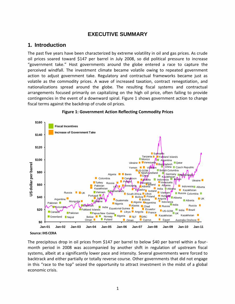
The past five years have been characterized by extreme volatility in oil and gas prices. As crude oil prices soared toward $147 per barrel in July 2008, so did political pressure to increase “government take.” Host governments around the globe entered a race to capture the perceived windfall. The investment climate became volatile owing to repeated government action to adjust government take. Regulatory and contractual frameworks became just as volatile as the commodity prices. A wave of increased taxation, contract renegotiation, and nationalizations spread around the globe. The resulting fiscal systems and contractual arrangements focused primarily on capitalizing on the high oil price, often failing to provide contingencies in the event of a downward spiral. Figure 1 shows government action to change fiscal terms against the backdrop of crude oil prices.

Figure 1: Government Action Reflecting Commodity Prices

$0

$20

$40

$60

$80

$100

$120

$140

$160

Jan-01 Jan-02 Jan-03 Jan-04 Jan-05 Jan-06 Jan-07 Jan-08 Jan-09 Jan-10 Jan-11

US

do

lla

r p

er

ba

rre

l

Colombia

Canada

Greenland

Pakistan

Nepal

Pakistan

Falkland Islands

Denmark

Papua New Guinea

Ukraine

India

NorwayPoland

Portugal

VietnamUK

UKPakistanKazakhstan

Turkey

OmanBelize

Nigeria

GuatemalaArgentina

Russia

ColombiaChina

Argentina

Algeria

Algeria

Alaska

Venezuela

Ecuador

Bolivia

Equatorial Guinea

PolandRussia

Cameroon

Algeria

Libya Angola

Alaska

Alberta

Newfoundland

T&T

Benin

BoliviaSpain

Oman

Mongolia

Chad

DRC

Iceland

Ireland

LibyaSouth Africa

France

Cyprus

Yemen Vietnam

Ukraine Venezuela

VenezuelaAlbania

Kazakhstan

Vietnam

Hungary

Indonesia

Russia

Egypt

Ecuador

Fiscal Incentives

Increase of Government Take

US-GOM

US-GOM

Alberta

British Columbia

Kazakhstan

China

Germany

Indonesia

UK

India

AlbertaAlberta

Brazil

Alberta

Colombia

UK

Russia

Kazakhstan

Australia Onshore

AngolaPoland

Colombia

Kazakhstan

Russia

Ukraine

Czech Republic

Netherlands

Netherlands

Bangladesh

Brunei

India

India

Indonesia

Argentina

Falkland IslandsMexico

Suriname

Qatar

Tanzania

Source: IHS CERA

The precipitous drop in oil prices from $147 per barrel to below $40 per barrel within a four-month period in 2008 was accompanied by another shift in regulation of upstream fiscal systems, albeit at a significantly lower pace and intensity. Several governments were forced to backtrack and either partially or totally reverse course. Other governments that did not engage in this “race to the top” seized the opportunity to attract investment in the midst of a global economic crisis.

2

In this “race to the top” or “race to the bottom,” depending on the perspective, governments share the same goal: developing the resource for the benefit of their citizens. Although the goal may be the same, the approaches and policies vary considerably. A nation’s energy policy is shaped by its economic development needs, relative prospectivity or resource size, dependence on hydrocarbon revenues, protection of the environment, and other factors. Government actions are a reflection of the way governments balance these policy objectives. The success or failure in this race is measured not by what position a given nation takes in a ranking of government take or other indexes, but rather by whether the nation has reached its policy objectives.

2. Objective of the Study

Bureau of Ocean Energy Management (BOEM) and Bureau of Land Management (BLM) commissioned this IHS CERA study to compare the oil and gas fiscal systems that apply on federally owned offshore and onshore lands with oil and gas fiscal systems adopted by other countries that compete with the United States for investments in the oil and gas upstream industry.

The purpose of the study is not to make recommendations but rather to inform decisions about lease terms on federal lands by providing a consistent comparison of selected federal oil and gas fiscal systems with those of other petroleum-producing countries. This comparative analysis and ranking is applied against current federal lease terms as well as against new models reflecting some of the suggested changes provided by the Department of the Interior (DOI) for future oil and gas leasing on federal lands. It is not within the scope of this study to make direct recommendations related to specific royalty rates or fiscal elements for federal leases.

This IHS CERA study compares 29 oil and gas upstream fiscal systems with respect to government share of profit, rates of return and other measures of profitability, revenue risk, and fiscal system stability in relation to each country’s policy objectives and oil and gas resource endowment.

3. About IHS CERA

IHS Cambridge Energy Research Associates, Inc. (IHS CERA) is a leading advisor to international energy companies, governments, financial institutions, energy consumers, and technology providers. IHS CERA delivers critical knowledge and independent analysis on energy markets, geopolitics, industry trends, and strategy. As part of IHS Inc. IHS CERA has access to the most comprehensive databases of oil and gas activity and analytical tools.

4. Approach

In assessing the competitive position of a fiscal system and its ability to strike the proper balance between attracting investment and generating appropriate returns to the resource holder, the size and availability of the oil and gas resources in place are crucial elements. To mirror each investment environment, IHS CERA relied on actual oil and gas discoveries made in each jurisdiction between 2000 and 2010. A total of 153 exploration and development cost models representing 124 conventional field developments and 29 unconventional oil and gas

3

projects were selected for this comparative review. This study relies on actual finding and development costs in each jurisdiction, taking into consideration varying commodity prices, price differentials, distance from liquid markets, the actual size of discoveries, well productivity, water depth, and technological challenges associated with each environment and resource type. This approach enables an “apples to apples” comparison of fiscal systems by generating models that mirror each investment environment.

A set of three West Texas Intermediate (WTI) prices was chosen, using as appropriate price differentials to account for crude quality. Distance from liquid markets is taken into account by netting back the price of crude oil to the wellhead, i.e., deducting the cost of transportation from the WTI price that has already been adjusted to account for the quality differential. For the purpose of this study we used a low price of $45 per barrel, a base price of $75 per barrel, and a high price of $105 per barrel.

The selection of natural gas prices becomes more complex owing to the lack of a global gas market. Natural gas trade is currently centered in three distinct regional markets: North America, Europe, and Asia.1 These markets have different degrees of maturity. The natural gas prices selected for each region reflect the market structures in the region. For North America the selected natural gas prices are $4 per Mcf, $6 per Mcf, and $8 per Mcf, netted back to the wellhead. Gas that is sold in European markets is analyzed at $6 per Mcf, $8 per Mcf, and $10 per Mcf. For Asia the selected natural gas prices are $8 per Mcf, $10 per Mcf, and $12 per Mcf, relying on the long-term liquefied natural gas (LNG) contract prices.

We developed three cost scenarios to match the low, base, and high price cases for each region. For the base case scenario, we used costs prevailing in third quarter 2010, i.e., $75 per barrel price, and the respective gas price for each region. High and low cost scenarios were developed using IHS CERA’s proprietary Capital Costs and Operating Costs Indexes based on the outlook to 2018 as of September 2010, when we began this study.

4.1 Finding the Right Peer Group

The federal fiscal systems are very diverse with respect to resource endowment, field discovery sizes, resource type (conventional versus unconventional), finding and development costs, E&P activity, industry players, and the components of oil and gas fiscal systems. To provide valid comparisons, the jurisdictions selected represent onshore and offshore development, North American and international, and conventional and unconventional resources.

Owing to significant differences in finding and development cost and the operation of different rentals and signature bonuses, the shelf and deepwater areas of the Gulf of Mexico have been treated as separate fiscal systems. Whereas onshore federal lands appear to have one applicable royalty rate, the application of state income and severance taxes and local property taxes results in several onshore fiscal systems on federal lands. For the purposes of this study the following federal fiscal systems were selected jointly by the DOI and IHS CERA:

U.S. Gulf of Mexico—shelf

U.S. Gulf of Mexico—deepwater

1

The European market includes Russia and North Africa.

4

U.S. federal lands—Wyoming conventional and unconventional gas

In short-listing the countries and the respective fiscal systems that were included in the study, a number of soft as well as numerical variables were established. Table 1 contains a list of the 29 fiscal systems selected based on the criteria described in this section.

Table 1: 29 Fiscal Systems Selected for Study

Fiscal System Location Fuel Type

Algeria Onshore conventional oil and gas

Australia (federal) Offshore conventional gas

Brazil Offshore conventional oil and gas

Canada (Alberta) oil sands Onshore oil sands

China Offshore conventional oil and gas

Germany Onshore shale gas

Indonesia coalbed gas Onshore coalbed gas

Kazakhstan Offshore conventional oil

Malaysia Offshore conventional oil and gas

Poland Onshore conventional and shale gas

United Kingdom Offshore conventional oil and gas

U.S. GOM deepwater Offshore conventional oil and gas

U.S. Louisiana (state lands) Onshore conventional and shale gas

U.S. Wyoming (federal lands) Onshore conventional and coalbed gas

Venezuela heavy oil Onshore heavy oil

Angola Offshore conventional oil and gas

Australia Queensland Onshore coalbed gas

Canada (Alberta) conventional oil Onshore conventional oil

Canada (British Columbia) Onshore shale gas

Colombia Onshore conventional oil and gas

India Offshore conventional oil and gas

Indonesia conventional Offshore conventional gas

Libya Onshore conventional oil and gas

Norway Offshore conventional oil and gas

Russia Onshore conventional oil and gas

U.S. Alaska (state lands) Onshore conventional oil and gas

U.S. GOM shelf Offshore conventional oil and gas

U.S. Texas (state lands) Onshore conventional oil and gas

Venezuela gas Onshore conventional gas

For the purpose of identifying the above jurisdictions that compete with the U.S. government for upstream oil and gas investment, the following E&P activity variables were selected:

The country has significant existing or potential production.

There has been significant exploratory activity in recent years.

5

The third and most important criterion in the numerical rating and ranking developed for this purpose is exploration success over the past five years.

To capture planned activity and future potential of the petroleum-producing countries, especially the potential for unconventional oil and gas resources, a 60 percent weighting was allocated to E&P activity of the past five years and a 40 percent weighting to E&P activity that is expected to take place in the next five years. The selection criteria combined global and regional comparisons, offshore versus North America onshore.2

5. Government Take on Federal Lands

The currently applicable royalty rate of 18.75 percent in the Gulf of Mexico has significantly increased government take compared with the rates referenced in 2008 by the United States Government Accountability Office (GAO) in it its report Oil and Gas Royalties: The Federal System for Collecting Oil and Gas Revenues Needs Comprehensive Reassessment.3 For shelf projects modeled for this study, the range of government take varies from 57 percent to 99 percent, with a fiscal system average of 79 percent.4 For the deepwater Gulf of Mexico the results of the study show that government take ranges from 53 to 90 percent, with a system average of 64 percent. In Wyoming, government take for gas resources ranges from 53 to 93 percent. Even though the current GOM shelf and deepwater fiscal systems are almost identical—the only difference lies in rental rates which usually are a rather minor component of government take and rarely have a noticeable impact on the overall government take percentage—the average government take varies significantly between them. The relatively small size of the recent discoveries on the shelf leads to a higher per-unit cost compared with the deepwater projects. This ultimately has an impact on the government take. Whereas this study shows that the government collects less revenue on a per-project basis from new discoveries on the shelf, the government take statistic tells a different story. For this reason, and others, government take reveals only part of the full picture.

Our economic analysis supports the arguments that the government take varies with commodity prices, finding and development costs, reserve size, reservoir characteristics, distance from infrastructure, water depth, and other factors. There is no single government take statistic, unless the regime is absolutely neutral. The wide ranges of government take between 53 percent for profitable projects to 86 percent for marginal ones in deepwater GOM suggest a highly regressive fiscal system that penalizes marginal fields.5 Figure 2 demonstrates

2 Saudi Arabia, Kuwait, Mexico, and Iran were eliminated owing to restricted foreign investment and information

being held confidential by the respective governments. Iraq was eliminated since the security issues that Iraq presents are not comparable with any of the other jurisdictions selected for review. Nigeria was also eliminated because oil and gas licensing in Nigeria has been at a stalemate for the past three years, pending approval of sector reforms that were introduced to the parliament in 2008. 3

U.S. Government Accountability Office, Oil and Gas Royalties: The Federal System for Collecting Oil and Gas

Revenues Needs Comprehensive Reassessment, GAO-08-691 (Washington, DC, September 2008). 4

In calculating averages, IHS CERA has eliminated projects that result in 100 percent government take under all three price and cost scenarios. For a detailed description of the approach, see Appendix III. 5

Under a regressive fiscal regime such as the U.S. federal fiscal systems, the government take declines as project profitability increases and increases as profitability declines. Such systems increase the marginal cost of development and often deter the development of marginal fields.

6

the cash flow components of Wyoming coalbed gas fields and the variance of government take with the variance of costs, reserve size, and reservoir characteristics. Although the government take for all five coalbed gas projects at a price of $6 Mcf is 66 percent, the range of government take for individual projects varies between 57 percent and 91 percent. The combined company income for all five coalbed gas projects is 15 percent of the combined cash flow, while the combined federal and state government income from all five projects is almost twice the amount accruing to the investor: 28 percent of the cash flow.

Figure 2: Government Take Variance in Five Coalbed Gas Fields

50%

73%

59%

58%59%

$0

$500

$1,000

$1,500

$2,000

$2,500

$3,000

$3,500

$4,000

$4,500

$5,000

Coalbed Gas Field 1

Coalbed Gas Field 2

Coalbed Gas Field 3

Coalbed Gas Field 4

Coalbed Gas Field 5

Mill

ion

Do

llars

Wyoming Coalbed Gas Fields

Government Take

Company Income

Income Taxes

Production Taxes

Royalty

Bonus and Rental

Operating Expenses

Capital Expenditure

Company Income 15% of Cash FlowGovernment Income 28% of Cash Flow66% Government Take

Source: IHS CERA

6. Fair Share

One of the policy objectives of the Outer Continental Shelf Lands Act (OCS Lands Act) is to assure receipt of fair market value for the offshore lands leased and rights conveyed by the federal government. The Mineral Leasing Act, which governs the oil and gas activities onshore, authorizes the Secretary of the Interior to set the minimum bid so as to enhance financial returns to the United States. To fulfill the mandate of the OCS Lands Act, BOEM follows specific bid adequacy procedures to ensure that the government receives fair market value for the tracts receiving offshore bids.6

The GAO made a finding that the U.S. government is not receiving a fair return on oil and gas leases in the GOM. That finding, however, appears to be based on a ranking of government take rather than an analysis of the bid adequacy procedures or an accounting of the amounts received via signature bonuses and income tax. Based on the ranges of the GOM government take reported by the GAO, we have concluded that the specific GOM government takes did not

6 This process is carried out in several phases and incorporates geological and geophysical data along with reserve,

resource, engineering, and economic information into a sophisticated discounted cash flow computer model. The goal of that model is to achieve estimates of fair market value on tracts receiving bids.

7

include signature bonuses or account for exploration risk.7 Studies that factored in risk and present value in the mid-1980s and late 1990s reported the U.S. OCS government take closer to 77 percent.8 If not accounted for in the government take statistic, a significant source of revenue accruing to the U.S. government is being overlooked.9

6.1 What Is Fair Share?

All the changes of fiscal terms introduced over the past five years have been based on the premise that the government is not receiving a fair share. Whether the change has been politically motivated, as in the nationalization of Venezuela’s oil industry, or purely for revenue collection purposes, as in Alberta, Alaska, Australia, Newfoundland and Labrador, and elsewhere, the question has always been the same: Is the government getting a fair share of the revenue from its oil and gas resources?

Although there is universal consensus that the government and the public should receive a fair share of the revenue from the oil and gas resources, there appears to be no standard or benchmark as to what that means. What is a fair share is a judgment or opinion that can neither be refuted nor proven.10 The Alberta Department of Energy in its 2007 Royalty Review recognized the inherently subjective nature of the fair share concept.11 Nonetheless, it concluded that Alberta was not receiving its fair share but without properly defining the benchmark or justifying the reasoning for such a conclusion. Fairness was judged on the basis that royalties had not changed for a long time rather than considering the fiscal system as a whole, taking into account that conventional resources had reached maturity or that Alberta’s royalty rates were among the highest in the world. Less than two years later, the government of Alberta reversed the royalty framework in order to maintain the competitive edge.12

Although concerns about whether the government is receiving a fair share of the oil and gas revenues over the long term may be more justified in a fiscal system where all components of the take are fixed, with fiscal systems relying on cash bonus bids for allocation of acreage, such as the federal oil and gas fiscal systems, the bonus bids create a self-correcting mechanism within the overall fiscal system.13 Since the bid value represents the economic rent the investors expect to receive from developing the resource, the investors can, within tolerable limits, reduce the amount of the bid if it is felt that the royalty or the government take is too high; likewise, investors may increase the bid amount under conditions where low royalties

7

In a phone interview with a GAO staff member in 2007, IHS CERA pointed out that the government take presented in that particular graph did not account for signature bonuses. 8Daniel Johnston, “Changing Fiscal Landscape,” Journal of World Energy Law and Business 1 (2008),1.

9 Ibid. See also Andrew Derman and Daniel Johnston, “Bonuses Enhance Upstream Fiscal System Analysis,” Oil and

Gas Journal, 51 February 8, 1999, 5. 10

Wade Locke, “Is Newfoundland and Labrador Getting Its Fair Share?” Newfoundland Quarterly 99, , no. 3 (2007). 11

Alberta Department of Energy, Royalty Information Briefing # 2—What is Fair Share?—Alberta Royalty Review

(2007), 1. 12

Government of Alberta, Energizing Investment: A Framework to Improve Alberta’s Natural Gas and Conventional Oil Competitiveness, (March 11, 2010). 13

Sierra Systems, Project Committee Final Report to the Alberta Department of Energy on Alberta’s Natural Gas and Conventional Oil Competitiveness, (2010), Appendix B-12.

8

leave more room for investors.14

Bonus bids in the U.S. OCS have acted as self-correcting mechanisms within the federal fiscal systems. During 2005–2010 revenue collected by the DOI from signature bonuses for the U.S. offshore constituted 27 percent of total revenue the DOI collected from offshore oil and gas leases. When each individual year is examined separately, there is clear evidence that in times of high prices investors have been willing to contribute a significant amount in signature bonuses.15 In 2008, when the oil price reached its highest at $147 per barrel, revenue from signature bonuses made up 53 percent of the total revenue collected by the DOI from OCS oil and gas leases. The $9 billion collected in signature bonuses alone far outweighed any hypothetical loss in royalty revenue because of a failure to introduce a sliding scale royalty to capture the upside.16 Figure 3 gives a breakdown of the DOI revenue from OCS oil and gas leases for the 2005–2010 fiscal years.

Figure 3: DOI OCS Revenue (Fiscal Year 2005–2010)

$0

$2,000

$4,000

$6,000

$8,000

$10,000

$12,000

$14,000

$16,000

$18,000

$20,000

2005 2006 2007 2008 2009 2010

Mil

lio

n D

oll

ars

Fiscal Year

Bonus

Rents

Royalty

Source: IHS CERA, data from ONRR

14

Sierra Systems, Project Committee Final Report to the Alberta Department of Energy on Alberta’s Natural Gas and Conventional Oil Competitiveness, (2010), Appendix B-12. 15

While the DOI does not rely on bonuses as a "self-correcting mechanism," but as a reflection of past choices on risk sharing, signature bonuses, have in fact acted as a self correcting mechanism for Gulf of Mexico. 16

In 2008 the GAO wrote “The Inflexibility of Royalty Rates to Changing Oil and Gas Prices Has Cost the Federal

Government Billions of Dollars in Foregone Revenues.” GAO, Oil and Gas Royalties,16. Given the time lag from award of acreage to first production (five to ten years), the U.S. government would not have been able to reap the benefits of any royalty revisions, even if such revisions were introduced in 2005.

9

Federal government revenue from onshore acreage in Wyoming shows a similar trend as the revenue from outer continental shelf acreage. Data on revenue collected in terms of signature bonuses, royalties, and rentals in federal lands in Wyoming show a 100 percent increase in revenue in 2008 from 2007 (Figure 4). However signature bonuses were not the source of additional revenue in times of high commodity prices. The adjusting mechanism in the case of Wyoming was investment in producing capacity. The relative ease with which new sources of supply are brought onstream onshore in the United States compared with offshore acreage led to increased investment in production capacity. While sales volumes of crude oil in Wyoming federal lands continued their steady decline despite the high commodity prices, sales volumes of processed residue gas increased 80 percent in 2008 compared with 2007.17 In 2010 as natural gas prices dropped to $4 Mcf from an average of $8 per Mcf in 2008 the sales volumes of processed residue gas dropped by 52 percent compared with 2008.18 This behavior is supported by the results of the economic analysis conducted for this study, which shows positive rates of return for only one out of five conventional gas fields selected from the pool of discoveries made in the past ten years.

Figure 4: DOI Wyoming Revenue (Fiscal Year 2006–2010)

$0

$200

$400

$600

$800

$1,000

$1,200

$1,400

$1,600

2006 2007 2008 2009 2010

Mil

lio

n D

oll

ars

Fiscal Year

Bonus

Rents

Royalty


17

According to data published on ONRR website sales volumes of crude oil produced from federal lands in Wyoming dropped from 29,844,078 barrels in 2007 to 28,556,565 barrels in 2008, while sales volumes for processed residue gas increased from 547,765,513 Mcf to 998,826,124 Mcf during the same period. 18

According to data published on ONRR website sales of processed residue gas in 2010 dropped to 522,711,425 Mcf, lower than the 2007 sales volume of 547,765,513 Mcf.

10

7. Resource Endowment

As a general trend, countries with high prospectivity, low development costs, and a stable investment environment should be able to demand higher levels of government take. Perceived endowment is a motivator for companies to invest in a particular jurisdiction, despite high levels of political risk or high levels of government take. What drives fiscal policy is often the government’s perception of its own endowment. Governments that have an unrealistic perception of their endowment often design fiscal policies that fail to attract investment.19 More than 150 jurisdictions have a petroleum fiscal system in place, although fewer than half of them have any significant production.20 Yet some of the toughest fiscal terms are found in jurisdictions with no established production. Having a fiscal system in place and demanding a high government take does not always establish a successful policy. For any ranking or competitiveness review to be meaningful, it is important to find the right peer group.

The analysis found that the U.S. jurisdictions in general, except for the deepwater GOM, ranked high with respect to the number of wells drilled; however, the size of the discoveries per new-field wildcat drilled was among the lowest. When drilling for shale is excluded, from the perspective of field sizes onshore jurisdictions in the United States were not as appealing as most of the countries selected for this study. Although a significant number of wells are drilled in the United States each year, they have very low productivity. Most of the conventional oil and gas fields discovered onshore in the United States are smaller than 1 million barrels of oil equivalent (MMboe).

When remaining reserves are taken into consideration, all three federal oil and gas jurisdictions ranked relatively low compared with Texas and other international oil and gas jurisdictions (see Figure 5). When comparing jurisdictions based on average government take among the cases generated for this study, all three federal jurisdictions are levying a higher government take than other jurisdictions relative to their remaining recoverable reserve ranking.

19

Robin Boadway and Michael Keen, “Theoretical Perspectives on Resource Tax Design” (paper presented International Monetary Fund Conference on Taxing Natural Resources: New Challenges, New Perspectives September 25–27, 2008), 12, argued that policymakers are “generally less well-informed of the geological and commercial circumstances at all stages of particular resource projects than are those who undertake the exploration, development and extraction.” 20

Out of 116 countries we examined in the IHS Petroleum Economics and Policy Solutions (PEPS) database that had one or more petroleum fiscal systems in place, 30 had no established production, with an additional group of 30 not having any significant production that would make them competitors of the United States.

11

Figure 5: Government Take Relative to Remaining Recoverable Reserve Ranking

Algeria

Angola

Australia offshore

Brazil China

Colombia

Germany

India

Indonesia

Kazakhstan Libya

Malaysia

Norway

Poland

Russia

United Kingdom

Venezuela heavy oil

U.S. GOM deepwater

U.S. GOM shelf

Louisiana

Texas

Alaska

Wyoming

Alberta oil sands

British Columbia

Queensland

Alberta conventional

Venezuela gas

0.00

0.50

1.00

1.50

2.00

2.50

3.00

3.50

4.00

4.50

5.00

0% 10% 20% 30% 40% 50% 60% 70% 80% 90% 100%

Re

ma

inin

g R

ec

ove

rab

le R

es

erv

e R

ati

ng

Average Government TakeSource: IHS CERA

8. Ranking of Fiscal Systems

Rather than relying on one single measure such as government take to compare fiscal systems, the study uses a composite index which includes indicators of profitability, measures of fiscal system flexibility, revenue risk, and fiscal stability. Reliance on a single indicator is unlikely to capture all dimensions of project economics and fiscal system competitiveness.

This study compares fiscal systems based on three main indexes:

Fiscal terms—combines comparison of government take statistics with profitability indicators such as internal rate of return (IRR) and measures of capital efficiency such as profit-to-investment ratio, as well as measures of fiscal system progressivity/regressivity, i.e., the ability of government take to increase or decline with increases or declines in project profitability. Each of the four variables is assigned an equal weight of 25 percent.

Revenue risk—analyzes the timing of revenue accruing to the government as a measure of risk sharing between resource owners and private investors.

Fiscal stability—focuses on changes in fiscal terms over the past five years and assesses stability of fiscal terms on the basis of

12

whether the change led to an increase or a decline of government take

whether the change applied to new investments or all investments

the degree of the change, considering the percentage increase in government take

frequency of the change

To provide consistent comparison and ranking of government take, rate of return, profit-to-investment ratio, and progressivity/regressivity of fiscal systems with other factors such as risk of return and flexibility and stability of fiscal systems, we developed a relative rating and ranking system which assigned each variable a score of zero to five, where a score of five indicates a high government take, highly progressive/regressive fiscal system, low rate of return to investors, low profit-to-investment ratio, low risk of return to the government, and unstable fiscal terms. On the other end of the spectrum a score of zero indicates low government take, high rate of return and profit-to-investment ratio, a neutral fiscal system, high risk of return to the government, and stable fiscal terms. Table 2 shows the variables under each category and their weight.

Table 2: Composite Index

Fiscal Terms Revenue

Risk Fiscal Stability

Weight

40% 30% 30%

Go

vern

men

t Ta

ke

Inte

rnal

Rat

e o

f R

etu

rn (

IRR

)

Pro

fit

to In

vest

men

t R

atio

(P

I)

Pro

gres

sivi

ty/R

egre

ssiv

ity

Tim

ing

of

Go

vern

men

t R

even

ue

Typ

e o

f C

han

ge

Ap

plic

abili

ty o

f C

han

ge

Deg

ree

of

Ch

ange

Fre

qu

ency

of

Ch

ange

Weight

25% 25% 25% 25% 100% 20% 30% 40% 10%

13

8.1 Ranking of Fiscal Terms

Analysis of government take shows that on average the take in the U.S. GOM shelf is higher than the worldwide average of 72 percent and the offshore average of 74 percent. 21 By itself, this metric fails to reveal whether the fiscal system is attractive to investors, or reflect the rather marginal nature of profits. The average PI at a discount factor of 10 percent is 0.72, which means that for every dollar invested, the total value created is $0.72. The IRR indicator also shows poor rates of return, averaging 4 percent. Even under our high price assumption of $8 per Mcf of gas and $105 per barrel of oil, the PI ratio and IRR remain rather low, at 0.89 and 8 percent, respectively.

In a ranking of offshore fiscal systems based on equal weighting of all four variables, the GOM shelf fiscal system is at the top of the list while the deepwater system ranks fifth. Reliance on bonus bids and high royalty rates for revenue collection has resulted in the balance weighing in favor of the government. Figure 6 shows the ranking of fiscal terms for offshore systems. A combination of low IRR and high government take and a highly regressive fiscal system is likely to result in loss of competitive edge for the GOM shelf fiscal system. While the deepwater fiscal system does not rank as high as the fiscal system applicable on the shelf, there is potential for the deepwater also to lose competitive ground, in particular with regard to natural gas resources.22 The fiscal system has also been shown to be vulnerable when commodity prices drop. This vulnerability was manifested in 2009 when there was a significant drop in acreage leased as well as bonus revenue from both areas of the gulf when commodity prices were low.

Figure 6: Fiscal Terms Index—Offshore

0.00 0.50 1.00 1.50 2.00 2.50 3.00 3.50 4.00 4.50

Australia offshore

Angola offshore

United Kingdom offshore

China offshore

Brazil offshore

India offshore

Kazakhstan offshore

U.S. GOM deepwater

Indonesia conventional gas offshore

Malaysia offshore

Norway offshore

U.S. GOM shelf

Fiscal Index Score

Gov Take PI IRR Progressivity/Regressivity

Source: IHS CERA

21

The average government take in the GOM shelf is 79 percent. 22

Our economic model revealed that a significant number of natural gas fields in deepwater areas of the Gulf of Mexico were subeconomic under the prevailing costs and commodity prices.

14

When all four variables are combined into a single index, Wyoming gas fiscal system ranks fifth among the seven onshore North American jurisdictions. Wyoming, however, faces strong competition from the Canadian jurisdictions of British Columbia and Alberta as well as from the United States jurisdictions with shale gas potential. As traditional sources of gas supply are displaced by the lower-cost shale gas resources, Wyoming could become less competitive. The trend of leasing and the average bonus bid per acre payable on federal lands in Wyoming is significantly lower than the amounts payable in the other jurisdictions, except Alaska.23 The high-cost conventional gas resources that were developed prior to 2008, when commodity prices were high, are no longer competitive under the prevailing market prices. Four out of five conventional fields modeled for Wyoming resulted in negative IRR. Figure 7 ranks North American onshore jurisdictions based on the fiscal terms index developed for this study.

Figure 7: Fiscal Terms Index—Onshore North America

0.00 0.50 1.00 1.50 2.00 2.50 3.00 3.50

Canada (British Columbia)

U.S. Louisiana onshore gas

U.S. Wyoming gas

Canada (Alberta) conventional oil

U.S. Alaska onshore

Canada (Alberta) oil sands

U.S. Texas onshore

Fiscal Index Score


Source: IHS CERA

Figure 8 shows the profitability indicators and government take for all 29 fiscal systems. A ranking of fiscal terms based on all four variables puts all U.S. federal jurisdictions in the top half of the index, which indicates high government take, low IRR, low PI, and highly regressive fiscal terms. The GOM shelf appears to be least favorable to investors among the U.S. jurisdictions, ranking in the top 10 percent, with Wyoming gas and the GOM deep water ranking in the top 35–50 percent range.

23

There has been a notable increase in bonus bids per acre in 2011 in Wyoming on a select number of parcels sold. This is associated with the potential for shale oil development in Niobrara, south of Wyoming. Although this has led to an increase of the average bonus bid per acre from $168 in 2010 to $474 in 2011 (as of October 2011), Wyoming continues to rank below Texas, British Columbia, and Louisiana in bonus bids per acre received in 2011.

15

Figure 8: Fiscal Terms Index

0.00 1.00 2.00 3.00 4.00 5.00

Poland onshoreAlgeria onshore

Canada (British Columbia)Australia (Queensland) coalbed gas

Australia offshoreAngola offshore

Indonesia coalbed gasUnited Kingdom offshore

U.S. Louisiana onshore gasLibya onshore

Colombia onshoreChina offshoreBrazil offshore

U.S. Wyoming gasIndia offshore

Kazakhstan offshoreCanada (Alberta) conventional oil

Russia onshoreU.S. GOM deepwater

Indonesia conventional gas offshoreGermany onshore

U.S. Alaska onshoreCanada (Alberta) oil sands

U.S. Texas onshoreVenezuela conventional gas

Malaysia offshoreNorway offshore

U.S. GOM shelfVenezuela heavy oil

Fiscal Index Score

Gov Take

PI

IRR

Progressivity/Regressivity

Source: IHS CERA

8.2 Revenue Risk

The high level of uncertainty associated with oil and gas exploration and development raises serious questions as to who should undertake the risk and to what extent the government should, as resource holder, share in the project risk. The sources of risk are varied, and they can occur at all stages of an upstream oil and gas venture. Some of the main risks associated with oil and gas exploration and development are as follows:

Geological and geophysical risks. These relate to the probability of finding substantial, technically and economically recoverable deposits. Such risks accompany all phases of an upstream venture. It is only when the deposit is fully exhausted that operators know precisely the size of the reserve.24

Price. Price volatility is one of the major risks that upstream oil and gas investments face throughout the project life. While high commodity prices may lead to significant upside, depressed prices can have a devastating impact on project economics and may at times cause the premature cessation of upstream activities.

24

Phillip Andrews-Speed, “Fiscal Systems for Mining: The Case of Brazil,” Journal of Mineral Policy, Business and Environment 13, no. 2, (1998), 13–21.

16

Cost. As commodity prices go up, the associated demand for goods and services usually drives the cost up. This definitely has an impact on project economics and, ultimately, the before-tax profit to be shared between the government and the investor.

Who should undertake the risk and in what measure is a policy decision.25 Whereas companies hedge against risk by investing in a diverse global portfolio of projects, governments hedge against risk by transferring part of it to the private investors.26 There is a fundamental conflict between the government and the oil companies over the division of risk and reward from an upstream oil and gas investment.27 Each party wants to maximize rewards and shift as much risk as possible to the other party. The choice and the design of the petroleum fiscal system reflect the trade-off between each party’s interests.

Table 3 displays the degree of risk exposure associated with each fiscal instrument.

Table 3: Revenue Risk of Fiscal Instruments

Fiscal Instrument Risk to Government

Bonus payments Low

Ad valorem payments (royalty, severance tax, export duty) Low

Cost recovery ceiling Low

Corporate income tax Medium

Resource rent tax High

Profit sharing Medium

Equity participation High

Source: IHS CERA

Risk-Reward Structure of Federal Fiscal Systems

Bonus Bids

The federal oil and gas fiscal systems rely heavily on bonus bids for allocation of acreage. These upfront payments for the right to explore and produce provide no guarantee that the lessee will be able to discover oil and gas in paying quantities, effectively shifting the risk of exploration onto the oil companies. The amount of bids payable depends largely upon

Perceived prospectivity of the jurisdiction. The relative maturity of a geological basin affects the level of competition and the size of the winning bids.28 This explains the

25

Silvana Tordo, David Johnston, and Daniel Johnston, “Countries’ Experience with the Allocation of Petroleum Exploration and Production Rights: Strategies and Design Issues,” World Bank Working Paper no. 179, (2007). 26

Ibid. 27

Emil M. Sunley, Thomas Baunsgaard, Dominique Simard, “Revenue from the Oil and Gas Sector: Issues and Country Experience,” (Background Paper prepared for the IMF Conference on Fiscal Policy Formulation and Implementation in Oil Producing Countries, June 5–6, 2002), World Bank. 28

Tordo, Johnston, and Johnston, Countries’ Experience with the Allocation of Petroleum Exploration and Production Rights, viii.

17

relatively lower amount of bids per acre received in Wyoming and the GOM shelf areas compared with the deepwater GOM.

Expected future oil and gas prices. Price expectations affect the number of bids as well as the bid size for the same geological basin. That partly explains the variability over time of the average bid per acre received for rights on federal lands. Thus, in 2007 and 2008, as the oil prices were steadily going up, the number of bids in the GOM and the average bid per acre were high, largely because of expectations that prices would persist at those levels or continue to go up. In 2009, the depressed commodity prices, combined with the global economic crises, contributed to a decline in total acreage sold as well as in the average bid per acre.29

Overall sharing of risks and rewards between government and investor. Depending on the design of the fiscal system and the degree of risk undertaken by the government, investors adjust their expected rate of return when they bid for acreage. Thus, in a fiscal system in which government revenue is front-end loaded, the investors are likely to seek a higher rate of return compared with a jurisdiction that allows the investors to recover costs and generate a specific rate of return before any revenue accrues to the government.

Royalty

Unlike bonuses that guarantee the resource holder revenue regardless of the success or failure of exploration efforts, revenue from royalties is tied to production or gross proceeds from oil and gas produced. In this respect royalties are not as regressive as bonuses, and the government shares the risk of exploration with the oil companies. However, royalties in general, and the ones applicable in the United States in particular, do not take into account the profitability of the oil and gas investment. Therefore they shift the price, cost, and reserve risk largely onto the oil companies. Whereas the total revenue accruing to the government is affected by commodity prices, the royalty rate is insensitive to production levels, price, or cost. Thus it can contribute toward an increase in the marginal cost of extracting oil and gas, and it can discourage the development of marginal fields or lead to early abandonment of oil and gas properties.

Income Tax

Revenue from upstream oil and gas investments is subject to corporate income tax. Unlike bonuses and royalties that present a low revenue risk for the federal government, the level of risk sharing increases with corporate income taxes. While the company bears the investment risk, the government shares in the revenue risk through allowable deductions and credits. Since income taxes are levied on profits, the government’s share of revenues is dependent on the project being profitable. The price, cost and reserve risk are shared between the government and investors. The total government revenue is sensitive to commodity prices, finding and development cost and production volumes.

29

See Table 5.4 for the decline in new acreage licensed in 2009.

18

8.2.1 Revenue Risk Index

To provide a consistent comparison of fiscal systems from the revenue risk perspective and to ascertain the extent to which governments share in the project risk, we examined what percentage of total government revenue was collected early on in the producing life of the field. To this end, we compared the revenue accruing to the government when the field reached one quarter of its producing life against the total revenue accruing to the government from each individual project. The share of government revenue early in the field life averaged around 7 percent in the case of Norway and 57 percent in the case of Angola. Relative risk scores of zero to five were assigned to each jurisdiction. The jurisdiction with the lowest revenue risk allocation to the government, i.e., where the government received the largest share of its total revenues early in the producing life, was assigned a score of five (in this case, Angola); the jurisdiction where the government undertakes the highest revenue risk through back-end loading of revenue (in this case, Norway) was assigned a score of zero. The other jurisdictions were assigned a relative score falling between the two extremes.

Except for British Columbia, where the government revenue is back-end loaded, the North American fiscal systems are designed with several front-end loaded levies that reduce significantly the government’s revenue risk. This risk allocation is largely because the U.S. onshore fiscal systems rely on a variety of front-end loaded payments, such as signature bonuses, royalties, rentals, and severance and production taxes. Thus, when a field reaches a quarter of its producing life, the federal (and state) government in Wyoming receive on average 45 percent of their total revenue from this field, leaving the investor very vulnerable to shifts in commodity prices throughout the project life. Figure 9 shows the revenue risk ranking of onshore North American jurisdictions.

Figure 9: Revenue Risk Ranking—Onshore North America

0.59

2.87

3.04

3.81

4.39

4.79

4.95

0.00 1.00 2.00 3.00 4.00 5.00 6.00




U.S. Wyoming gas


U.S. Alaska onshore

U.S. Texas onshore

Revenue Risk ScoreSource: IHS CERA

19

Compared with all onshore jurisdictions covered in this study, the North American jurisdictions, including Wyoming federal lands, allocate the least degree of risk to the government. As with onshore fiscal systems, under the GOM fiscal systems the risk is allocated to the investor; however, the impact is not as harsh as in onshore U.S. jurisdictions because of the lack of severance and property taxes offshore. Compared with other offshore jurisdictions, the GOM fiscal systems fall in the top 50 percent, with the deepwater fiscal system ranking fourth out of 12 jurisdictions. Figures 10 and 11 display the revenue risk ranking of onshore and offshore jurisdictions covered in this study.

Figure 10: Revenue Risk Ranking—Worldwide Onshore

0.59

0.91

1.80

1.85

1.91

2.05

2.15

2.61

2.87

2.90

3.04

3.43

3.81

4.39

4.79

4.92

4.95

0.00 1.00 2.00 3.00 4.00 5.00 6.00


Poland onshore

Algeria onshore

Colombia onshore

Australia (Queensland) coalbed gas

Libya onshore

Indonesia coalbed gas

Germany onshore


Venezuela heavy oil


Russia onshore

U.S. Wyoming gas


U.S. Alaska onshore

Venezuela conventional gas

U.S. Texas onshore

Revenue Risk ScoreSource: IHS CERASource: IHS CERA

20

Figure 11: Revenue Risk Ranking Worldwide Offshore

0.00

0.28

0.73

1.78

1.86

2.18

2.38

2.51

2.71

2.74

3.44

5.00

0.00 1.00 2.00 3.00 4.00 5.00 6.00

Norway offshore



Malaysia offshore

India offshore

Australia offshore

U.S. GOM shelf

China offshore

U.S. GOM deepwater

Kazakhstan offshore

Brazil offshore

Angola offshore


8.3. Fiscal Stability

When considering where to invest, investors often consider the stability and predictability of the prevailing fiscal and regulatory environment. Stability affects the confidence of investors in government policy.30 A fiscal system that is subject to frequent change increases political risk and reduces the value placed by investors on future income streams.31 Oil price volatility has brought instability to oil and gas fiscal systems. The desire to capture the upside when commodity prices are high has resulted in a competitive race to increase government take and assert greater control over natural resources.

This fiscal stability index takes into account all the various measures introduced by governments around the globe and assigns risk scores from zero to five to each fiscal system depending on the type of change (increase versus decrease of the fiscal burden), the applicability of change (application to future investments versus all investments or renegotiation of existing contracts), the degree of change, and the frequency of change.

The four categories of stability identified in this study have been combined to provide useful and consistent comparison among the jurisdictions covered. Each variable has been assigned a specific weight. As with any weighting system these weights are subjective. Decision makers and investors may assign different weights to each variable depending on their perception of

30

Carole Nakhle, Petroleum Taxation: Sharing the Oil Wealth: A Study of Petroleum Taxation, Yesterday, Today, and Tomorrow, (New York: Routledge 2008), 161. 31

Nakhle, Petroleum Taxation.

21

risk and their ability to manage such risk. Table 4 shows the specific weights assigned to each variable of the fiscal stability index in this study.

Table 4: Fiscal Stability Index Weights

Fiscal Stability

Type of Change Applicability of Change Degree of Change Frequency of Change

30% 20% 40% 10%

Among the offshore jurisdictions, Kazakhstan and the United Kingdom show the highest degree of instability over the past five years. They are followed by Brazil and the deepwater GOM. Unlike in Kazakhstan and the United Kingdom, the changes introduced in Brazil and for the deepwater GOM apply to future terms only and therefore do not have an impact on existing investments. However, they have resulted in significantly increased government take and could impact an investor’s ability to participate in future lease offerings. The degree of change in government take has been the highest in the United Kingdom, Brazil, and the deepwater GOM. Brazil’s increase in government take is spurred by the significant spike in prospectivity. The changes in the United Kingdom and United States, however, are not associated with any major shifts in prospectivity. They appear to be simply motivated by the desire to capture a larger share of the before-tax profits. Figure 11 shows the ranking of jurisdictions under the fiscal stability index.

Figure 12: Fiscal Stability Index

0.00 1.00 2.00 3.00 4.00 5.00 6.00

India offshore


U.S. GOM shelf

Angola offshore

Australia offshore

Poland onshore


China offshore

U.S. GOM deepwater

Colombia onshore

Brazil offshore


Algeria onshore

U.S. Alaska onshore


Kazakhstan offshore


Russia onshore

Libya onshore

Venezuela heavy oil

Fiscal Stability Score


Note: British Columbia, Germany, Indonesia CBG, Louisiana, Malaysia, Norway , Texas, Venezuela Conventional Gas and Wyoming have a zero score and have not been included in this chart.

Source: IHS CERA.

22

8.4 Composite Index

A combination of the index of fiscal terms, revenue risk, and fiscal stability captures various dimensions of project economics and fiscal system competitiveness. A comparison of offshore fiscal systems shows that both Gulf of Mexico fiscal systems rank very favorably from a government perspective, indicating high government take, low rates of return and profit-to-investment ratio, low revenue risk for the government, and somewhat unstable fiscal terms. The other OECD countries whose policies are more aligned with the policies of the United States, mainly the United Kingdom, Norway, and Australia, provide a more attractive investment environment than the U.S. government. These governments undertake a higher revenue risk, owing largely to profit-based or resource rent levies that expose the government to greater risk when projects are not profitable and reward them with a greater share of the upside when profitability increases. Figure 13 shows a ranking of offshore fiscal systems based on the composite index.

Figure 13: Composite Index—Ranking of Offshore Systems

0.00 0.50 1.00 1.50 2.00 2.50 3.00

Norway offshore


Australia offshore


India offshore

Malaysia offshore

China offshore

U.S. GOM deepwater

Brazil offshore

U.S. GOM shelf

Angola offshore

Kazakhstan offshore

Final Index Score

Gov Take

PI

IRR

Progressivity/Regresivity

Revenue Risk

Type of Change

Applicability of Change

Degree of Change

Frequency of Change

Source: IHS CERA

Government Perspective

Investor Perspective

Wyoming natural gas fiscal systems ranks fifth among the seven North American fiscal systems. The relatively high government take combined with the rather low revenue risk taken by the government is offset by the fiscal stability score to provide a relatively attractive environment for investors. The scores of Wyoming should be interpreted with caution since a significant number of the conventional gas fields were excluded from the calculation of average indicators under the assumption that they will not be developed in the current price and cost

23

environment. See Appendix III, Tables III–V.a and b, and III-VI for an explanation of the approach and the individual field results. Figure 14 shows a ranking of onshore North American fiscal systems based on the composite index.

Figure 14: Composite Index—Ranking of Onshore North American Fiscal Systems

0.00 0.50 1.00 1.50 2.00 2.50 3.00 3.50 4.00



U.S. Wyoming gas


U.S. Texas onshore


U.S. Alaska onshore

Final Index Score

Gov Take

PI

IRR


Revenue Risk

Type of Change


Degree of Change

Frequency of Change

Source: IHS CERA



The overall ranking of the 29 fiscal systems shows the U.S. GOM shelf, U.S. GOM deepwater, and U.S. Wyoming gas fiscal systems ranking tenth, twelfth, and fifteenth, respectively. On a global perspective the North American jurisdictions in general, and the federal fiscal systems in particular, reap most of the rewards and share very little revenue risk compared with the majority of the jurisdictions included in this study. 32, 33 Figure 15 shows the overall ranking of the 29 fiscal systems under the composite index.

32

The exception is British Columbia, which has designed a back-end loaded fiscal system for shale gas resources whereby the government undertakes a significant share of the revenue risk. 33

The only revenue risk exposure is through federal and state income taxes.

24

Figure 15: Composite Index—Global Rating and Ranking

0.00 0.50 1.00 1.50 2.00 2.50 3.00 3.50 4.00 4.50


Poland onshore

Norway offshore



Australia offshore


Algeria onshore

India offshore

Malaysia offshore

Colombia onshore

Germany onshore



U.S. Wyoming gas

China offshore


U.S. GOM deepwater

Brazil offshore

U.S. GOM shelf

Libya onshore

Angola offshore

U.S. Texas onshore

Kazakhstan offshore



Russia onshore

U.S. Alaska onshore

Venezuela heavy oil

Final Index Score

Gov Take

PI

IRR


Revenue Risk

Type of Change


Degree of Change

Frequency of Change

Source: IHS CERA



9. Alternative Fiscal Systems

One of the objectives of this study is to compare alternative fiscal systems suggested by the DOI against its existing fiscal systems as well as those of other jurisdictions. The objective is not to make recommendations but rather to inform policy decisions.

The alternative rates suggested by the DOI consist of a range of flat rate royalties as well as one sliding scale royalty. The following flat rate royalties have been suggested by the DOI for onshore as well as offshore areas:

12.5% 18.75% 20% 25%

The suggested sliding scale royalty rates are tied to commodity prices starting at a low threshold of $30 to $150 per barrel for crude oil and from $3 to $11 per Mcf for natural gas. Table 5 summarizes the suggested sliding scale royalty rates for offshore and onshore federal lands.

25

Table 5: Alternative Sliding Scale Royalty Rates

Commodity Price Onshore Offshore

Oil $30 per barrel 12.50% 12.50% $45 per barrel 16.67% 16.67% $74 per barrel 18.75% 18.75% $105 per barrel 22.50% 21.88% $150 per barrel 22.50% 31.25%

Gas $3 per Mcf 12.50% 12.50% $4 per Mcf 12.50% 16.67% $6 per Mcf 16.67% 18.75% $8 per Mcf 18.75% 21.88% $11 per Mcf 18.75% 31.25%

The royalty reduction alternative for the GOM, as expected, results in a reduction of average government take by 8 and 9 percent, respectively, for deepwater and shelf areas. This measure does improve the profitability indicators; however, the measure is not sufficient to improve the profitability of the mature resources of the shelf to reasonable levels that would encourage investment. The gas-prone areas of the shelf face competition from the lower-cost supplies associated with shale gas development onshore in the United States and Canada. The 12.5 percent rate lowers the degree of regressivity of the GOM fiscal systems, but they remain highly regressive. Table 6 shows the average government take, PI ratio, investor IRR, and degree of regressivity of the alternative offshore fiscal systems compared with the status quo.

Table 6: Average Indicators for Alternative Royalty Rates in the Gulf of Mexico

Royalty Government Take PI IRR Progressivity/Regressivity

U.S. GOM Deepwater

12.50% 55% 1.11 11% -14%

18.75%* 64% 1.04 10% -18%

20.00% 65% 1.02 10% -17%

25.00% 72% 0.96 8% -18%

Sliding Scale 65% 1.02 10% -7%

U.S. GOM Shelf

12.50% 70% 0.77 5% -13%

18.75%* 79% 0.72 4% -16%

20.00% 80% 0.71 4% -17%

25.00% 85% 0.66 3% -18%


Source: IHS CERA *Currently applicable rate.

When the royalty rate increases from 18.75 percent to 20 percent, any appreciable benefit that accrues from the 2 percent revenue increase is offset by eroding rates of return and a

26

heightened perception of instability. Although royalty rates of 20 to 25 percent are not common in offshore oil and gas exploration and production, the GOM nominal royalty rate is already higher than that of all offshore oil and gas jurisdictions outside the United States. Other offshore jurisdictions such as the United Kingdom, Norway, and Australia, albeit with high government takes, do not levy royalties for new acreage.

When compared against other North American jurisdictions, the flat alternative rate royalty systems will make Wyoming gas projects less attractive than Louisiana, British Columbia, and Alberta conventional oil. These jurisdictions, however, are home to some of the most prolific shale gas resources in North America, offering alternative, lower-cost, new sources of supply.

The sliding scale royalty appears to result in no significant benefit to the federal government compared to the status quo: a 1 percent increase. It does, however, depress the already low profitability indicators, bringing the average investor IRR below 10 percent. When the full impact of the sliding scale is analyzed, i.e., economics are run to incorporate crude oil prices of $30 per barrel and $150 per barrel, which represent the lowest and the highest price thresholds under the suggested alternative, the results for the sliding scale royalty are harsher than the 25 percent royalty alternative for the GOM. In the case of Wyoming, the results of the sliding scale fall between those of the 20 and 25 percent royalty alternative. Although the fiscal system becomes less regressive, which influences the overall index score, the introduced flexibility does not influence investment decisions when profitability falls below acceptable hurdle rates.34

The lower overall score for the sliding scale is largely attributed to its flexibility as it adjusts with commodity prices. The sliding scale royalty has been designed to capture the upside; however, it does not offer any relief from the current fiscal system for Wyoming when natural gas prices are low. A 12.5 percent floor royalty rate is high for a jurisdiction that is geologically the least attractive compared to the other North American jurisdictions. Indeed, that is clear from the oil and gas industry’s appetite to bid on Wyoming federal lands. The average bids per acre in Wyoming are the second lowest, next to Alaska among the select peer group. Figure 16 shows the average bids per acre paid since 2006 in the various jurisdictions.35

A significant number of jurisdictions internationally offer lower royalties or other incentives for natural gas. Among the countries reviewed in this study, China, Colombia, Venezuela, Russia, Kazakhstan and Poland apply lower royalties for natural gas, Even in North America, the Canadian provinces of Alberta and British Columbia have established floor royalty rates for natural gas starting at 5 percent and 2 percent, respectively. A 12.5 percent royalty rate when gas prices are at or below $3 per Mcf does not offer flexibility in the fiscal system for either onshore or offshore acreage and thus does not make the fiscal systems more attractive to investors.

34

Studies conducted by Alberta Royalty Review Panel and industry experts involved in the hearings held during the revision of Alberta’s royalty framework in 2007 held rates of return between 13 percent and 20 percent and PI ratios between 1.15 and 1.75 to be acceptable profitability thresholds. See Pedro Van Meurs, “Preliminary Fiscal Evaluation of Alberta Oil Sands Terms,” presented to the Alberta Department of Energy, April 12, 2007. 35

The bids per acre do not distinguish by resource. When new acreage is awarded it is not necessarily classified as oil, gas or shale. In some cases there may be more than one resource type underlying the lease tract.

27

Figure 16: Average Bid per Acre Onshore North America

2006 2007 2008 2009 2010

Louisiana $377.33 $527.94 $2,321.65 $1,107.16 $1,239.17

British Columbia $358.54 $691.33 $1,383.37 $902.27 $871.16

Texas $413.74 $267.66 $366.16 $277.97 $869.21

Alberta $214.91 $149.28 $182.28 $165.31 $243.66

Wyoming $46.67 $62.06 $77.44 $24.64 $167.85

Alaska $22.86 $15.72 $25.00 $25.89 $14.78

$0

$500

$1,000

$1,500

$2,000

$2,500

Bo

nu

s B

id p

er A

cre

(US$

)

Source: IHS CERA

The approach and the rating and ranking for this task are the same as with those developed for the current fiscal terms comparison. The alternative fiscal systems do not significantly change the sharing of risks and rewards between the government and investors. This is largely because the structure and the components of the fiscal system remain unchanged. The sliding scale royalty, sometimes referred to as a “progressive royalty,” does very little to change risks and rewards. The progressive royalty rates linked to commodity prices do not make the fiscal system progressive. Any potential increase in revenue risk to the government resulting from the reduced royalty rate when commodity prices decline is offset by a lowering of the risk resulting from the increase of royalty rate when commodity prices rise. Therefore there is no discernible difference in revenue risk sharing between the sliding scale royalty and the status quo for the GOM shelf areas.

On a global scale, the introduction of alternative royalty rates higher than the status quo, such as the 20 and 25 percent rates for offshore and 18.75, 20, and 25 percent royalty rates for onshore, place the federal fiscal systems at the top of the ranking chart and contribute to a diminished competitive position. Despite the risk of instability, the introduction of a 12.5 percent royalty rate significantly improves the attractiveness of the GOM fiscal systems. However, this rate reduction may not prove sufficient to bring the GOM marginal fields onstream. When other factors such as resource potential, potential reduction in revenue

28

collected via signature bonuses and income tax, and the comparable royalty rates for the specific environment are factored in, the alternative royalty rates suggested for this study could deter investment and in turn affect timely resource development, which could ultimately lead to reduced federal revenue. Figure 17 shows the overall ranking of alternative fiscal systems under the composite index.

Figure 17: Composite Index: Alternative Fiscal Systems—Global Ranking

0.00 1.00 2.00 3.00 4.00 5.00

Canada (British Columbia)Poland onshore

Norway offshoreIndonesia coalbed gas

Indonesia conventional gas offshoreAustralia offshore

United Kingdom offshoreAlgeria onshore

India offshoreMalaysia offshoreColombia onshoreGermany onshore

U.S. GOM deepwater 12.5% royaltyAustralia (Queensland) coalbed gas

U.S. Louisiana onshore gasU.S. Wyoming gas

China offshoreU.S. GOM shelf 12.5% royalty

U.S. GOM deepwater sliding scale …U.S.Wyoming gas sliding scale royalty

Canada (Alberta) conventional oilU.S. GOM deepwater

U.S. GOM deepwater 20% royaltyBrazil offshoreU.S. GOM shelf

Libya onshoreAngola offshore

U.S. GOM shelf sliding scale royaltyU.S. GOM shelf 20% royalty

U.S. Wyoming gas 18.75% royaltyU.S. Texas onshore

Kazakhstan offshoreVenezuela conventional gas

U.S.Wyoming gas 20% royaltyU.S. GOM deepwater 25% royalty

Canada (Alberta) oil sandsU.S. GOM shelf 25% royalty

U.S.Wyoming gas 25.5% royaltyRussia onshore

U.S. Alaska onshoreVenezuela heavy oil

Index Score

Gov Take

PI

IRR


Revenue Risk

Type of Change


Degree of Change

Frequency of Change

Source: IHS CERA



10. Conclusion

Government take should not be the only measure to determine attractiveness of the fiscal system. If it is used at all, it should be combined with other measures of profitability, fiscal system flexibility, revenue risk, and fiscal stability in order to properly assess petroleum fiscal systems. Such analysis should be combined with a proper understanding of the resource potential and the relative prospectivity of the federal lands. Fiscal design should be a reflection of the jurisdiction’s relative prospectivity, economic development needs, dependence on hydrocarbon revenues, and environmental protection policies. This study found that all three federal jurisdictions are levying a higher government take than other jurisdictions relative to their remaining recoverable reserve ranking.

From a resource-size perspective, Wyoming federal lands conventional resources cannot

29

compete with Gulf of Mexico and international jurisdictions selected for this comparative analysis. Because of the size of natural gas fields likely to be discovered in Wyoming, the reserves per new-field wildcat, well productivity, and prevailing natural gas prices in the United States, Wyoming does not appeal to the oil and gas investors likely to invest internationally. In that respect, any ranking of Wyoming in global indexes developed for this study may not be as meaningful, as it is not within its peer group.

When compared with a peer group of North American jurisdictions, Wyoming’s competitive edge is on shaky ground. The province of Alberta and British Columbia are aggressively seeking to attract investment in conventional and unconventional gas resources in two ways: by offering incentives through lower initial royalty rates that encourage development or through net profit royalties that back-end government revenue and allow investors reasonable returns. If shale gas continues to perform better than expected, it could drive the higher-cost resources developed during the high price era that ended in 2008 off the margin. The current royalty rates on federal land do not reflect the maturity of the basins and the high cost of bringing these supplies to market. Although Wyoming may rank more favorably than some of the onshore jurisdictions in North America, its resource base and the high per-unit cost of development of its gas resources make it less appealing to investors, even if paying less on a dollar-per-acre basis for acquisition of acreage in Wyoming compared with Texas or Louisiana.

Exploration for and development of natural gas resources in the GOM face the same challenge as the exploration for and development of gas resources in Wyoming. They are a higher-cost alternative to shale gas resources being developed in North America. The current fiscal system on the shelf does not reflect the maturity of the resource. Royalties levied on federal lands in the GOM are the highest among offshore jurisdictions surveyed for this analysis. Therefore they increase the marginal cost of development, discouraging the development of the GOM’s high-cost deep and ultradeep natural gas resources. This is reflected in the rather high ranking of the GOM fiscal systems compared with other offshore and onshore jurisdictions.

The bonus bid system adopted by the federal government is an objective and fair way to allocate acreage. Since the bid value represents the economic rent investors expect to receive from developing the resource, the bonus bid serves as a self-correcting mechanism within the fiscal system. In times of high commodity prices, revenue from bonus bids in Outer Continental Shelf lands has exceeded revenue collected through royalties and rentals combined.

Any increase of the already high royalty rate levied in the GOM will increase the risk of system instability. Any potential gains from the higher royalty rate are likely to be offset by reduced revenue from signature bonuses and the slower pace of leasing.

The 12.5 percent royalty alternative improves the competitive position of the GOM fiscal systems by placing them in the middle of the select peer group. Any of the suggested alternative rates for Wyoming federal lands, however, will deteriorate their competitive position in the market, which is rather weak as it is.

The sliding scale alternatives have been designed to capture the upside, providing no significant relief at the lower end of the scale. The 12.5 percent minimum royalty rate for commodity prices of $30 per barrel and $3 per Mcf is rather high, given that break-even prices at 10

30

percent discount are in the $70 per barrel range for the GOM jurisdiction.36 The added benefit of flexibility is not really a benefit when the fiscal system is designed simply to capture the upside. Most sliding scale royalties for natural gas adopted in other jurisdictions start at a rate of zero or 2 to 3 percent. A minimum 12.5 percent royalty rate for a sliding scale that exceeds 30 percent at the high end is rather high compared to other offshore jurisdictions.

36

The 12.5 percent royalty rate is the minimum rate established under OCSLA and the Department of Interior cannot lower the threshold without amendment of the statute.

31

1. CONTEXT AND SCOPE

In 2008 the United States GAO published Oil and Gas Royalties: The Federal System for Collecting Oil and Gas Revenues Needs Comprehensive Reassessment.37 The report, which suggests that the U.S. government’s return on federal oil and gas leases is lower than the returns of other resource owners, calls for a reassessment of the federal oil and gas fiscal systems. It states that the DOI does not routinely evaluate the oil and gas fiscal system, monitor what other governments or resource owners are receiving for energy resources, or evaluate and compare the attractiveness of federal lands and waters for oil and gas investment with that of other oil and gas regions.

The GAO considered it essential to evaluate the oil and gas fiscal system and to monitor what other governments or resource owners are receiving for their energy resources so as to determine whether there is a proper balance between the attractiveness of federal leases for investment and appropriate returns to the federal government for oil and gas resources. To this end the Bureau of Ocean Energy Managementand the Bureau of Land Management commissioned this IHS CERA study to compare the oil and gas fiscal systems that apply on federally owned offshore and onshore lands with oil and gas fiscal systems adopted by other countries that compete with the United States for investments in the oil and gas upstream industry.

The purpose of the study is not to make recommendations but rather to inform decisions about lease terms on federal lands by providing a consistent comparison of selected federal oil and gas fiscal systems with those of other petroleum-producing countries. This comparative analysis and ranking is applied against current federal lease terms as well as against new models reflecting some of the suggested changes by the DOI for future oil and gas leasing on federal lands. It is not within the scope of this study to make direct recommendations related to specific royalty rates or fiscal elements for federal leases.

1.1 Approach

Quite often comparative analysis of fiscal terms, including government take, is conducted by applying different fiscal systems to a hypothetical field or set of fields and comparing the resulting economic indicators and level of government take. Other studies have relied on a set of fields from the oil and gas jurisdiction that is the focus of the study and have applied other fiscal systems to the selected development concept. Although both approaches have their usefulness in the sense that they are able to analyze the behavior of fiscal systems under the same set of circumstances, they oversimplify the situation by assuming a world devoid of varying climates, topographies, and reservoir conditions, not to mention market conditions (including distance to liquid markets).

The GAO report recognizes the shortcomings of the above-mentioned approaches and

37

GAO, Oil and Gas Royalties.

32

emphasizes the need to take into consideration the size and availability of the oil and gas resources in place; the costs of finding and developing these resources, including labor costs and the costs of complying with environmental regulations; and the stability of the oil and gas fiscal system in particular and of the country in general. These factors were taken into consideration in defining the approach for this study, which is consistent with previous studies conducted by IHS CERA involving comparison of petroleum fiscal systems.38

1.1.1 Size and Availability of the Oil and Gas Resources in Place

In assessing the competitive position of a fiscal system and its ability to strike the proper balance between attracting investment and generating appropriate returns to the resource holder, the size and availability of the oil and gas resources in place are crucial elements. A comparison of fiscal systems on hypothetical oil and gas field sizes that are not likely to be found in the respective jurisdictions is theoretical at best and has limited applicability. To mirror each investment environment, IHS CERA relied on actual oil and gas discoveries made in each jurisdiction between 2000 and 2010. A total of 153 exploration and development cost models representing 124 conventional field developments and 29 unconventional oil and gas projects were selected for this comparative review. Appendix I contains an explanation of field selection criteria.

The IHS international, U.S., and Canadian proprietary exploration and production (E&P) databases were used to provide field information related to cumulative production, recoverable reserves, geological formation, reservoir and water depth, well flow rates, pressure, oil/gas ratio, distance from existing facilities and infrastructure, exploration success, and other inputs. The following data sets were used:

IHS Oil & Gas Discoveries and Fields databases cover more than 24,600 discoveries and 51,500 reservoirs.

IHS Wells Dataset provides comprehensive information on more than 680,000 international wells as well as over 3.5 million current and historical well records in the United States, accounting for virtually every well drilled and produced back to 1859.

IHS Oil & Gas Production Data in its various forms contains production data for over 115 countries, from country level down to field level, with annual and monthly information.

1.1.2 Finding and Development Costs

This study relies on actual finding and development cost in each jurisdiction, taking into consideration varying commodity prices, price differentials, distance from liquid markets, the actual size of discoveries, well productivity, water depth, and technological challenges associated with each environment and resource type. This approach enables an “apples to

38

Similar IHS CERA studies available in the public domain include the IHS CERA Special Reports A Comparison of Fiscal Regimes: Offshore Natural Gas in Israel (Cambridge, MA: 2010), http://www.mof.gov.il/BudgetSite/Reform/Lists/List9/Attachments/43/novelEnergy_4.pdf and A Comparison of Fiscal Regimes (Cambridge, MA: 2007). http://lba.legis.state.ak.us/aces/doc_log/2007-11-10_cera_a_comparison_of_fiscal_regimes_presented_to_sen_fin.pdf.

http://www.mof.gov.il/BudgetSite/Reform/Lists/List9/Attachments/43/novelEnergy_4.pdf

http://lba.legis.state.ak.us/aces/doc_log/2007-11-10_cera_a_comparison_of_fiscal_regimes_presented_to_sen_fin.pdf


33

apples” comparison of fiscal systems by generating models that mirror each investment environment.

IHS proprietary cost-modeling software QUE$TORTM was used for the development of cost models. QUE$TOR™ is the world’s leading software solution for new oil and gas project cost analysis. It is the industry standard tool for cost evaluation and concept optimization of new oil and gas field developments. QUE$TOR™ has been benchmarked against actual project costs and is continuously maintained to reflect the latest changes in technology. QUE$TOR uses primary input data including recoverable reserves, gas and liquid ratios, reservoir depth, and water depth. It leverages IHS basin data to generate a production profile that supports the development of concept and design flow rates.

To mirror the current investment environment, we modeled fields according to development concepts typical for each jurisdiction, using third quarter 2010 cost databases. Although the discoveries of the past ten years are useful for indicating the size and quality of the discoveries likely to be found in each jurisdiction, applying current costs provides insight about the cost of bringing similar discoveries onstream today.

The cost models account for abortive exploration efforts, applicable risk premiums associated with each jurisdiction, and the cost of environmental compliance. IHS data on exploration success rates for each jurisdiction were used to account for the number of exploratory wells included in each model. The cost models used for this study provide detailed information on capital expenditure and operating costs, tangible and intangible expenditure, and processing and transportation costs, which are often allowed as deductions for royalty purposes.

The economics were run in real terms to avoid the need to make assumptions about escalation rates for capital and development costs. The models do not account for price escalation or inflation. We developed three separate price and cost scenarios to analyze the impact of varying market conditions on project economics.

1.1.3 Price and Cost Scenarios

The high degree of volatility in crude oil markets over the past five years is an indication of the uncertainty that surrounds oil and gas investments, which ultimately has an impact on the revenue accruing to the resource holder. The selection of crude oil prices for this analysis is not intended as a forecast but rather reflects the relatively wide gap between the high and low price ranges that have prevailed since 2008, the year with the most dramatic shift in crude oil prices in the past decade.39

A set of three West Texas Intermediate (WTI) prices was chosen, using appropriate price differentials to account for crude quality. Distance from liquid markets is taken into account by netting back the price of crude oil to the wellhead, i.e., deducting the cost of transportation from the WTI price that has already been adjusted to account for the quality differential. For the purpose of this study, we used a low price of $45 per barrel, a base price of $75 per barrel, and a high price of $105 per barrel. The base price represents the average WTI price for the 12-

39

In 2008 the average monthly WTI price reached a high of $134 per barrel in June–July and a low of $41 per barrel toward the end of the year.

34

month period preceding the date this study was commissioned. The low and the high prices vary by (-/+)$30 per barrel from the base price and represent the average prices for November 2008–April 2009, which was marked by predominantly low crude oil prices, and for October 2007–October 2008, which was marked by predominantly high oil prices.

The selection of natural gas prices becomes more complex owing to the lack of a global gas market. Natural gas trade is currently centered in three distinct regional markets: North America, Europe, and Asia.40 These markets have different degrees of maturity. In North America, spot and derivative markets are fully developed. Despite the emerging natural gas hubs in Europe, that market relies more heavily on long-term contracts, with price terms indexed to a mix of competing fuels. Asia favors long-term contracts, with the natural gas price indexed to the crude oil price. These market structures have resulted in higher natural gas prices in Europe and Asia than in North America.

Applying one set of natural gas prices across the board would not reflect the business environment in the selected jurisdictions. In determining the range of gas prices applicable in North America, we relied on historical Henry Hub prices published by the U.S. Energy Information Administration (EIA). The 2008–10 period was marked by a high price of $8 per Mcf and a low price of $4 per Mcf. Hence, for North America, the selected natural gas prices are $4 per Mcf, $6 per Mcf, and $8 per Mcf, netted back to the wellhead.

Gas that is sold in European markets is analyzed at $6 per Mcf, $8 per Mcf, and $10 per Mcf. The prices selected represent a balance between the spot price and the term contract prices in Europe. The $6 per Mcf price represents the average U.K. National Balancing Point (NBP) gas price for January 2010–September 2010.41 Historical term contract prices in Europe between 2008 and 2010 ranged between $7 and $12 per Mcf. We selected the $10 per Mcf average for this period for the high price scenario and $8 per Mcf as the base price.

Long-term liquefied natural gas (LNG) contract prices in Asia have been just as volatile as crude oil prices. Average annual prices since 2008 ranged between $7 and $17 per Mcf, with monthly average prices skyrocketing in July 2008 to $22 per Mcf. For this study, we relied on the average $8 per Mcf price prevailing in the second half 2010 for the low case scenario and the combined average of 2008 and 2009 prices of $12 per Mcf for the high price scenario, with $10 per Mcf for the base case, which reflects the 2011 prices in the region. The cost of liquefaction and transportation of LNG from Australia, Indonesia, and Malaysia into China and Japan was reflected in the netback prices for the respective models. IHS CERA’s LNG Analytics Application was used to determine the cost of liquefaction and transportation into the respective markets.42

We developed three cost scenarios to match the low, base, and high price cases for each region. Since 2000, upstream capital costs have skyrocketed; however, they do not exhibit the

40

The European market includes Russia and North Africa. 41

The NBP, a virtual trading location for natural gas in the United Kingdom, is the most liquid gas trading hub in Europe. 42

The LNG Analytics Application is an interactive tool providing critical information and economic analysis on the global LNG business through a unique combination of comprehensive data, forward-looking IHS CERA projections across markets, and project economics analysis tools.

35

same degree of volatility as commodity prices. Figure 1.1 shows the movement of the WTI spot index and the IHS CERA Upstream Capital Costs Index (UCCI) in 2000–11 and their divergence since 2008.

Figure 1.1: Crude Oil and Upstream Capital Costs Indexes

50

100

150

200

250

300

350

400

450

2000 2001 2002 2003 2004 2005 2006 2007 2008 2009 2010 2011

WT

I Sp

ot

Ind

ex

& U

CC

I In

de

x (

20

00

=1

00

)

IHS CERA Upstream Capital Costs Index Average WTI Spot Indexed

Source: IHS CERA

For the base case scenario, we used costs prevailing in the third quarter 2010, i.e., $75 per barrel and the respective gas price for each region. High- and low-cost scenarios were developed using IHS CERA’s proprietary Capital Costs and Operating Costs Indexes based on the outlook to 2018 as of September 2010, when we began this study.

The IHS CERA UCCI and Upstream Operating Costs Index (UOCI) track the costs of operations equipment, facilities, materials, and personnel (both skilled and unskilled) used in the construction of a geographically diversified portfolio of onshore, offshore, pipeline and LNG projects. They are similar to the Consumer Price Index (CPI) in that they provide a clear, transparent benchmark tool for tracking and projecting a complex and dynamic environment.

The UCCI and UOCI track the purchase price and the “life-cycle cost” for a representative set of project portfolios and calculate weighted values for various inputs that have caused upstream project costs to skyrocket in recent years. The indexes account for factors such as

engineering, procurement, and construction labor scarcity

operations labor scarcity

number of current well projects

rig rates, spares, chemicals, helicopters, vessels, and power

36

raw materials supply: availability of premium steel, cement, copper, and diesel fuel

competition with downstream industry for resources

1.1.4 Finding the Right Peer Group

In comparing oil and gas fiscal systems it is important to identify the right peer group. The U.S. fiscal systems in general and the Gulf of Mexico region in particular have often been included in studies conducting a comparative review of fiscal terms. They have been included in worldwide comparisons, regional comparisons focused mainly in the United States or North America, and comparison of systems with similar technological challenges and cost environments.

1.1.4.1 Worldwide Approach

The worldwide approach involves comparison of a rather significant number of fiscal systems (over 100 in most cases) without specifically targeting a particular fiscal system as the focus of the analysis. Often such studies do not distinguish between jurisdictions with established production and an active E&P sector and those that aspire to attract investment, or the ones that have failed to attract investments over a considerable period of time or are closed to private equity investments. Though they provide useful theoretical information, the findings of such studies can be misleading when the analysis focuses on comparison of government take statistics and fails to identify the jurisdictions where the government is not generating any revenue at all or where its revenue is dwindling as a result of the fiscal or energy policies in place. Another shortcoming of studies of such broad scope is that they often make very general assumptions with respect to cost and field sizes and ignore the reality of the investment environment in each jurisdiction.

1.1.4.2 Regional Comparisons

Regional studies are usually justified when the petroleum jurisdiction is not competing in the international market for investments, i.e., the size of the resource or the market conditions are such that investment in the respective jurisdiction would not appeal to companies with a diversified portfolio of domestic and international investments. It is not uncommon for an oil and gas jurisdiction to rely on international comparisons for a particular resource type and on regional comparisons for another. The government of Alberta in recent studies relied on international comparisons of high-cost investment environments for its oil sands resources; however, it limited the analysis of its mature conventional oil and gas resources to North American jurisdictions.43

1.1.4.3 Similar Cost Environments

When analysis of the fiscal system relies solely on “government take” as a comparative measure, the selection of similar cost environments is important to provide a consistent basis for comparison. The pretax profitability of activities in low-cost environments leaves more room than a high-cost environment for government take without undermining the

43

Alberta Royalty Review Panel. Our Fair Share: Report of the Alberta Royalty Review Panel (2007); and Sierra Systems, Appendix B-12.

37

attractiveness of investment in exploration and development of the hydrocarbon resources. When the resource holder is not considering measures of profitability, such as the IRR, profit-to-investment ratio, the expected monetary value, or other profitability criteria, this approach may be the most suitable one. However, this approach does to some extent overlook that investors have a global portfolio and may very well forgo the opportunity to invest in a high-cost jurisdiction in favor of a low-cost jurisdiction that offers higher rates of return, even if the high-cost jurisdiction ranks very favorably among other jurisdictions with similar cost structures.

1.1.4.4 IHS CERA Fiscal System Selection Criteria

The federal fiscal systems are very diverse with respect to resource endowment, field discovery sizes, resource type (conventional versus unconventional), finding and development cost, E&P activity, industry players, and the components of oil and gas fiscal systems. To provide valid comparisons, the jurisdictions selected represent onshore and offshore development, North American and international, and conventional and unconventional resources.

Owing to significant differences in finding and development cost and the operation of different rentals and signature bonuses, the shelf and deepwater areas of the Gulf of Mexico have been treated as separate fiscal systems. Whereas onshore federal lands appear to have one applicable royalty rate, the application of state income and severance taxes and local property taxes results in numerous onshore fiscal systems on federal lands. For the purposes of this study the following federal fiscal systems were selected jointly by the DOI and IHS CERA:

U.S. Gulf of Mexico—shelf

U.S. Gulf of Mexico—deepwater

U.S. federal lands—Wyoming conventional and unconventional gas

In short-listing the countries and the respective fiscal systems that were included in the study, a number of soft as well as numerical variables were established. For the purpose of identifying countries that compete with the U.S. government for upstream oil and gas investment, the following E&P activity variables were selected:

The country has significant existing or potential production. Although the level of production is important in analyzing the success or failure of a government’s fiscal policy in attracting investment in its jurisdiction, it is not a very strong indicator of recent policy decisions because of the long lead times from acquisition of mineral rights to first production. Since the high production levels do not often equate with future prospectivity, this criterion was assigned a 10 percent weight. The category was further divided into the following subcategories:

o oil production

o gas production

There has been significant exploratory activity in recent years. The level of recent exploration activity is often a better reflection of energy policy and fiscal measures adopted by a certain jurisdiction. The immediate impact of policy decisions is often

38

reflected in licensing and exploratory drilling. At that stage of the E&P life cycle, investors either have made no investment commitment, as in the case of licensing activity, or have committed very little in signature bonuses and other lease acquisition payments. Thus, their decisions to invest in new licenses or exploratory drilling are a better reflection of the opportunity cost of capital. As a consequence, any policy decisions, such as changes in fiscal terms that shift a country’s competitive position in the world, have a bearing on a country’s ability to attract new investments in the oil and gas sector. This criterion was given a 40 percent weighting in the overall scorecard. The level of exploratory activity is further measured by the following criteria:

o number of new field wildcats drilled

o number of licenses/contracts awarded in recent years

o number of E&P companies active in the country

The third and most important criterion in the numerical rating and ranking developed for this study is exploration success over the past five years. This criterion is crucial since a country’s perceived prospectivity and therefore decisions for future investments are based largely on exploratory successes or failures of recent years. This criterion is given a 50 percent weighting in the overall scorecard. The exploration success category is further measured by the following criteria:

o oil reserves added

o gas reserves added

o exploration success rate

o reserves added per new-field wildcat44

Although the ranking of E&P activity over the past five years is a good approach to identifying countries that have established E&P over a significant period of time, it fails to identify the countries that are emerging as competitors for future investments. The technological revolution that has enabled the development of unconventional gas resources in North America has put on the map of competitors for future investment some countries that in the past were not considered traditional oil and gas jurisdictions. To capture planned activity and future potential of the petroleum-producing countries, especially the potential for unconventional oil and gas resources, a 60 percent weighting was allocated to E&P activity of the past five years and a 40 percent weighting was allocated to E&P activity that is expected to take place in the next five years. Table 1.1 contains a graphical layout of the three main criteria and the defining set of variables.

44

A new-field wildcat is a well located on a structural feature or other type of trap that has not previously produced oil or gas.

39

Table 1.1: E&P Rating and Ranking Approach

OVERALL E&P

RATING

PERIOD OF ACTIVITY

WEIGHT MAIN CRITERIA WEIGHT VARIABLES WEIGHT

E&P

Act

ivit

y

E&P Activity,

Past Five Years

60% Production 10% Oil 60%

Gas 40%

Exploration Activity 40% New-Field Wildcat 50%

New Licenses 25%

Active Companies 25%

Exploration Success 50% Oil Reserves Added 20%

Gas Reserves Added 15%

Success Rate 15%

Reserves Added per New-Field Wildcat

50%

Expected E&P Activity, Next Five Years

40% Production 40% Oil 60%

Gas 40%

Exploration Activity 60% New Licenses 70%

Active Companies 30%

In addition to the above-mentioned numerical criteria, a set of soft (hard to quantify) criteria was used to narrow the list of fiscal systems, to provide adequate coverage without redundancy or excessive detail. The following are some of the softer criteria:

There is sufficient information available to enable analysis of a country’s fiscal system. This process resulted in elimination of the following jurisdictions from the comparative analysis:

o These countries were eliminated owing to restricted foreign investment and information being held confidential by the respective governments: Saudi Arabia, Kuwait, Mexico, and Iran.

o Iraq was eliminated from the list, not because it is not an important competitor for oil and gas investments, but rather because there has been no consensus regarding the new petroleum law, and the security issues that Iraq presents are not comparable with any of the other jurisdictions selected for review.

o Nigeria was also eliminated from the list of countries to compare against because oil and gas licensing in Nigeria has been at a stalemate for the past two years, pending approval of sector reforms that were introduced to the parliament in 2008.

The application of the above-mentioned numerical and soft criteria resulted in the selection of the following countries for comparative analysis:

Algeria Angola Australia

Brazil Canada China

Colombia Germany India

40

Indonesia Kazakhstan Libya45

Malaysia Norway Poland

Russia United Kingdom United States

Venezuela

In addition to international comparisons the analysis focuses on two subsets of peer groups:

Offshore jurisdictions. The U.S. Gulf of Mexico federal jurisdictions are compared against other offshore jurisdictions such as Angola, Australia, Brazil, China, India, Indonesia conventional gas, Kazakhstan, Malaysia, Norway, and the United Kingdom. Owing to the high cost involved with offshore development, most jurisdictions offer more lenient terms for offshore and deepwater acreage. This comparison is especially important in considering the specific components of government take, the mixture of front-end loaded payments with progressive back-end loaded ones, and the suitability of the alternative royalty rates for the specific environment.

Onshore North American jurisdictions. The maturity of conventional oil and gas resources in North America, as evidenced by the size of new-field wildcat discoveries over the past ten years; the competition for investment in unconventional resources; and the existence of an integrated natural gas network between the United States and Canada provide the basis for the selection of a subset of jurisdictions competing for investment with onshore federal jurisdictions, represented by Wyoming in this study.46 This peer group consists of Alaska, Alberta, British Columbia, Louisiana, and Texas. The significant role these jurisdictions’ peer group will play in the oil and gas sector in North America, the level of activity, and the fiscal instruments adopted by the respective jurisdictions were also a factor in the selection process. The DOI was interested in the diverse fiscal instruments adopted by these jurisdictions.

Upon consideration of the location of activities, the predominant fuel type, and the various fiscal systems applicable within each jurisdiction, 29 fiscal systems were selected.47 Table 1.2 displays a list of selected jurisdictions.

In conducting this analysis, we relied on information from the IHS Petroleum Economics and Policy Solution Service (PEPS). The service, which has been in existence for 25 years, provides analysis of petroleum legislation and fiscal systems of over 150 jurisdictions worldwide. Appendix II contains a brief summary of the fiscal terms used for the economic analysis.

45

The selection of the jurisdictions was made in September 2010, prior to the conflict in Libya. 46

Major gas pipelines in Canada interconnect with the U.S. pipeline grid at about a dozen export points. Canada contributes a significant portion to the natural gas supply of the United States. According to EIA, US natural gas consumption in 2010 was 24,133 billion cubic feet (Bcf), while imports from Canada for the same year were 3,275 Bcf, representing 14 percent of total consumption. This interdependence of the Canadian and U.S. natural gas markets has resulted in one integrated market where market pressures in one region are transmitted to the other regions. 47

Separate fiscal systems apply to conventional oil and oil sands in Alberta, to natural gas and heavy oil in Venezuela, and to conventional gas and coalbed gas in Indonesia.

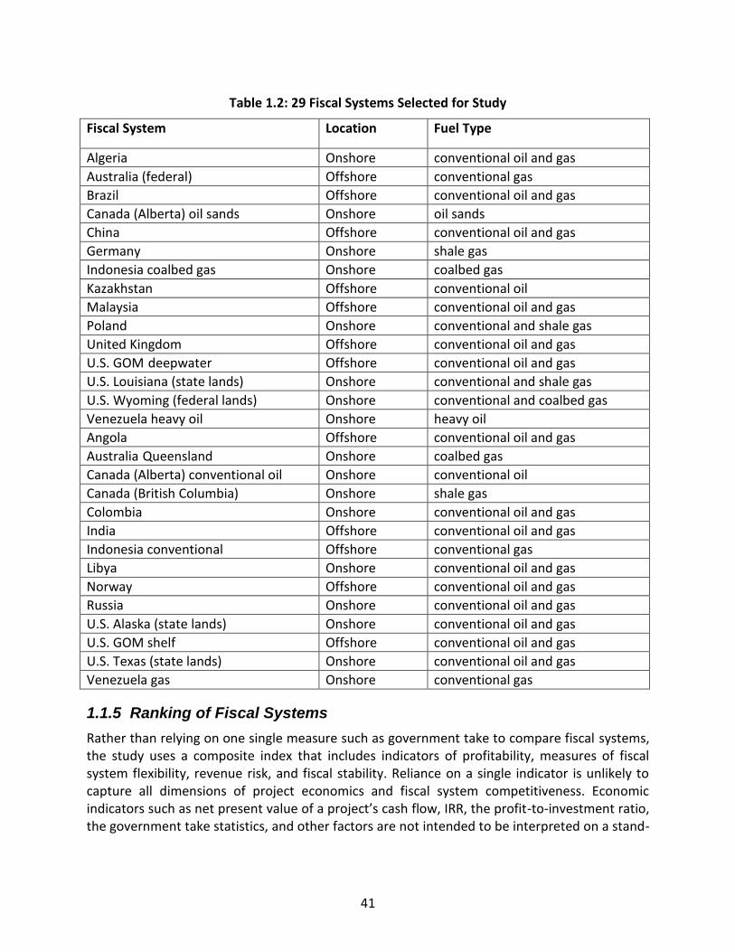
41

Table 1.2: 29 Fiscal Systems Selected for Study

Fiscal System Location Fuel Type

Algeria Onshore conventional oil and gas

Australia (federal) Offshore conventional gas

Brazil Offshore conventional oil and gas

Canada (Alberta) oil sands Onshore oil sands

China Offshore conventional oil and gas

Germany Onshore shale gas

Indonesia coalbed gas Onshore coalbed gas

Kazakhstan Offshore conventional oil

Malaysia Offshore conventional oil and gas

Poland Onshore conventional and shale gas

United Kingdom Offshore conventional oil and gas

U.S. GOM deepwater Offshore conventional oil and gas

U.S. Louisiana (state lands) Onshore conventional and shale gas

U.S. Wyoming (federal lands) Onshore conventional and coalbed gas

Venezuela heavy oil Onshore heavy oil

Angola Offshore conventional oil and gas

Australia Queensland Onshore coalbed gas

Canada (Alberta) conventional oil Onshore conventional oil

Canada (British Columbia) Onshore shale gas

Colombia Onshore conventional oil and gas

India Offshore conventional oil and gas

Indonesia conventional Offshore conventional gas

Libya Onshore conventional oil and gas

Norway Offshore conventional oil and gas

Russia Onshore conventional oil and gas

U.S. Alaska (state lands) Onshore conventional oil and gas

U.S. GOM shelf Offshore conventional oil and gas

U.S. Texas (state lands) Onshore conventional oil and gas

Venezuela gas Onshore conventional gas

1.1.5 Ranking of Fiscal Systems

Rather than relying on one single measure such as government take to compare fiscal systems, the study uses a composite index that includes indicators of profitability, measures of fiscal system flexibility, revenue risk, and fiscal stability. Reliance on a single indicator is unlikely to capture all dimensions of project economics and fiscal system competitiveness. Economic indicators such as net present value of a project’s cash flow, IRR, the profit-to-investment ratio, the government take statistics, and other factors are not intended to be interpreted on a stand-

42

alone basis.48 Since each indicator has its own limitations, they need to be carefully interpreted to account for such limitations, i.e., things they do not show.49 A combination of indicators is necessary for adequate comparison and assessment of fiscal systems.

Studies related to comparison of petroleum fiscal systems have often relied on analysis of various criteria and indicators; however, results have often been examined individually rather than combined.50 This study compares fiscal systems based on three main indexes:

Fiscal terms—combines comparison of government take statistics with profitability indicators such as after-tax rate of return to investors and measures of capital efficiency such as profit-to-investment ratio, as well as measures of fiscal system flexibility, i.e., the ability of government take to increase or decline with increases or declines in project profitability. Each of the four variables is assigned an equal weight of 25 percent.

Revenue risk—analyzes the timing of revenue accruing to the government as a measure of risk sharing between resource owners and private investors. This index distinguishes between fiscal systems where the government bears relatively low revenue risk compared with investors and those where the government bears a larger share of the revenue risk.

Fiscal stability—focuses on changes in fiscal terms over the past five years and assesses stability of fiscal terms on the basis of

whether the change lead to increase or decline of government take

whether the change applied to new investments or all investments

the degree of the change, considering the percentage increase in government take

frequency of the change (several jurisdictions changed the terms more than once during the past five years)

To provide consistent comparison and ranking of government take, rate of return, profit-to-investment ratio, and progressivity/regressivity of fiscal systems with other factors such as risk of return and flexibility and stability of fiscal systems, we developed a relative rating and ranking system that assigned each variable a score of zero to five, where a score of five indicates a high government take, highly progressive/regressive fiscal system, low rate of return to investors, low profit-to-investment ratio, low risk of return to the government, and stable fiscal terms. On the other end of the spectrum, a score of zero indicates low government take,

48

Silviana Tordo. Fiscal Systems for Hydrocarbons: Design Issues, World Bank Working Paper No. 123 (2007), 18.

49 Philip

Daniel, et al. 2006. Evaluating Fiscal Regimes for Resource Projects: An Example from Oil Development,

presented at IMF Conference on Taxing Natural Resources: New Challenges and New Perspectives, September 25, 2006. 50

Alberta Royalty Review Panel; Van Meurs Corporation, Comparative Analysis of Fiscal Terms for Alberta Oil Sands

and International Heavy and Conventional Oils (2007); Brenton Goldsworthy, and Daria Zakharova, Evaluation of the fiscal regime in Russia and proposals for reform, IMF Working Paper 10/33 (2010); Michael Alexeev, and Robert Conrad, “The Russian Oil Tax Regime: A Comparative Perspective,” Eurasian Geography and Economics 50, no. 3, 93–114; Mark J. Kaiser and Allan G. Pulsipher, 2004. Fiscal System Analysis: Concessionary and Contractual Systems Used in Offshore Petroleum Arrangements, U.S. Department of the Interior, Minerals Management Service, Gulf of Mexico OCS Region, New Orleans, LA. OCS Study MMS 2004-016.

43

high rates of return and profit-to-investment ratios, a neutral fiscal system, high risk of return to the government, and unstable fiscal terms. Figure 1.2 shows the variables under each category and their weight.

Figure 1.2: Composite Index Variables

Index VariablesIndex CategoriesTotal Jurisdiction

Score

Jurisdiction Score

Fiscal Terms

Government Take

P/I

IRR


Revenue Risk Timing of Revenue

Fiscal Stability

Type of Change

Nature of Change

Degree of Change

Frequency of Change

Weighted Score40 % weight

30 % weight

30 % weight

25%

25%

25%

25%

100%

20%

30%

40%

10%

1.2 Organization of the Report

This report is organized into ten chapters. Chapter 2 provides a high-level overview of petroleum fiscal systems, focusing mainly on the concept of government take, the main fiscal instruments found in petroleum fiscal systems analyzed for this study, limitations of government take, a review of the GAO report that was the instigator for this study, and other studies referenced in the GAO report.

Chapter 3 identifies factors influencing government take and investment decisions. This chapter examines what role, if any, resource endowment, political risk, and policy goals play in the design of fiscal policies for upstream oil and gas investments in the respective jurisdictions and the main drivers behind investment decisions.

Chapter 4 focuses on comparative analysis of fiscal terms such as government take, profit-to-investment ratio, internal rate of return, and the flexibility of fiscal designs. Using the methodology developed for this study, fiscal systems are ranked on the basis of each individual metric as well as on the basis of a composite index of fiscal terms.

Chapter 5 reviews the mechanisms in place for the sharing of revenue risk between host governments and investors and applies the study methodology for ranking of countries based on the front-end and back-end loading of the revenue stream to the resource holder.

Chapter 6 examines the long-term nature of upstream oil and gas investments, highlights the

44

need for stability, provides case studies for investor reaction to changes in government take, and ranks jurisdictions based on stability of fiscal terms over the past five years.

Chapter 7 brings together all the elements of profitability, flexibility, government take revenue risk, and fiscal stability into a composite index that rates and ranks each variable on a zero to five point system placing the government and investor perspectives on opposite ends of the spectrum.

Chapter 8 provides a detailed analysis of the fiscal systems resulting from the suggested royalty rates on federal lands in the U.S. onshore and offshore. This chapter examines the impact of each fiscal system on the various indicators developed for this study as well as the shift in ranking among the respective peer groups. The commodity prices required to reach break-even at 10 and 15 percent post-tax rate of return on investment is analyzed to provide insight into the cost of bringing onstream new sources of supply under the existing and suggested alternative royalty rates.

Chapters 9 and 10 make recommendations related to future updates and present study conclusions.

45

2. DESIGN OF PETROLEUM FISCAL SYSTEMS

2.1 Overview

With the exception of the United States and parts of Canada, where there is a combination of public and private ownership of mineral resources, oil and gas resources in the rest of the world are owned by the public. Depending on the institutional framework within each jurisdiction, the right to explore for and develop oil and gas resources is granted by the government through the ministry of energy, a government agency established to administer mineral rights, or through the national oil company (NOC).

Mineral rights are granted through either a concessionary or a contractual right. The concessionary system, or royalty/tax system as it is often referred to, is the older of the two.51 It has been adopted for oil and gas rights by 121 countries at one point in time or another.52 This is the fiscal system used in the United States. Contractual rights fall into two distinct categories: production sharing and service agreements. The latter can be further classified as pure service contracts and risk service contracts. Though use of service contracts in their pure form or as hybrids has been more limited (15 countries experimented with hybrids at one time or another), production sharing agreements (PSAs) have been just as widely used as concessionary ones (in 99 countries worldwide).53

Countries have various reasons for choosing one fiscal system over the other.54 Quite a few countries have tried all three, with a small number of jurisdictions providing for the application of more than one fiscal system in their petroleum legislation. Each type of right establishes the ground rules for the long-term relationship between the host government and the investor, including title to hydrocarbons, the degree of control granted to investors, the revenue-sharing mechanism, and any potential NOC involvement. The relationship can become fragile when the assumptions upon which it was established undergo major change. Restoring the balance is not always easy and often comes with resistance.55

Although the legal nature of rights granted and the degree of investor control in the decision-making process varies among concessions, PSAs, and service contracts, from a revenue-sharing

51

The concessionary regime has been in existence since 480 BC, when it was used by the Greek state for silver mining. See Owen L. Anderson, “Royalty Valuation: Should Royalty Obligations Be Determined Intrinsically, Theoretically, or Realistically?” Natural Resources Law Journal 37 (Summer 1997), 611. 52

Information has been assembled from historical evolution of contract terms within IHS Petroleum Economics and Policy Solutions (PEPS) service. 53

IHS PEPS.

54 The choice of the fiscal system often has deep roots in the culture, history, and sociopolitical condition of each

jurisdiction. See C Nakhle, Petroleum Taxation: Sharing the Oil Wealth: A Study of Petroleum Taxation Yesterday, Today and Tomorrow (Routledge, New York 2008), 48. Service contracts are often adopted in jurisdictions where the constitution prohibits the grant of title to hydrocarbons to private investors. 55

IHS CERA. E&P Fiscal Terms: Larger Pies but Smaller Portions, IHS CERA Decision Brief (2007); Thomas W. Waelde, and George Ndi, “Stabilizing International Investment Commitments: International Law Versus Contract Interpretation,” Texas International Law Journal 31, no.2 (1996), 216. Waelde and Ndi argue that there is a predominance of international energy and mineral arbitration cases compared with other sectors.

46

perspective the same result can be achieved under any of the three major types of contracts.

Depending on the fiscal instruments used and the number of variables attached to each levy, fiscal system designs can range from simple, efficient, and easy to administer to rather complex and difficult to administer. The desire to account for various contingencies has quite often resulted in rather complex fiscal designs that governments find difficult to audit and administer.56 Intelligent fiscal design without the institutional structures to support it may not achieve the desired goals.57 Fiscal design needs to be within the administrative capacity of the institutions managing and enforcing it. Sometimes the added cost of administering the design far outweighs any benefits associated with its enhanced capability to account for changes in project profitability, price, production volume, and other factors, especially if the design encourages tax avoidance or inefficient development of the resource.

In designing fiscal systems, governments often have to balance the desire to maximize revenue in the short term against the long-term goal of maximizing investments. Striking the right balance is not always easy. On numerous occasions governments find that what they perceive to be fair does not correspond with what the market considers fair. The market test is often the best test for the fairness of a fiscal system.58 However, that test is not without risk. If the market is tested too often, the system becomes unstable, and the lessons learned usually come with a significant price tag—lost investment and inefficient resource development. Sometimes loss of investor confidence arises after one or two instances of increase in government take such as in Alberta, Canada, and the state of Alaska, where changes introduced in 2007 led to deleterious impacts on investment levels.59 Nations that have shown a high degree of instability by changing fiscal terms with each fluctuation of the commodity price have suffered longer-term consequences—migration of investors away from the jurisdiction. In 2009 the number of active companies in Kazakhstan’s oil and gas sector dwindled to 71, from 143 in 2006, despite the government’s attempt to lower government take toward the end of 2008.60 Stable fiscal systems that encourage efficient resource development maximize the magnitude of revenue to be shared between the host government and the investor.61

56

See United Nations Conference on Trade and Development (UNCTAD). 1996. Administration of petroleum fiscal regimes. The study emphasizes that much of the complexity often arises out of government attempts to fully satisfy too many objectives, of both the host governments and the transnational oil companies. The problem that the study illustrates is that in an effort to encourage marginal field development, capture a fair share of "windfall profits," stimulate reinvestment of capital, earn the highest possible government take, and at the same time encourage exploration of most of the nation´s petroleum potential, governments are likely to design extremely complex fiscal systems. 57

Tordo, Fiscal Systems for Hydrocarbons, 15. 58

Sunley, Baunsgaard, and Simard, Revenue from the Oil and Gas Sector, 19. 59

Subsequent to introduction of Alaska’s Clear and Equitable Share (ACES) (petroleum profits tax introduced under the administration of Governor Sarah Palin) investment in Alaska dropped to levels not seen since oil prices were below $20 per barrel. Since entry into force of the new royalty framework (2009) licensing of new acreage for oil sands in Alberta dropped by more than 90 percent compared with 2008 levels. 60

IHS PEPS. 61

Tordo, Fiscal Systems for Hydrocarbons, 13-15.

47

2.2 The Concept of Government Take

2.2.1 Definition and Use of Government Take

Government take is a fiscal statistic often used by host governments in comparing fiscal systems. Academics and consultants often use it to compare fiscal systems, in particular to compare changes resulting from a recent or proposed change in taxation. Investors on the other hand rely on economic indicators such as net present value, rate of return, profit-to-investment ratio, the expected monetary value of exploration prospects, and other factors rather than government take to make investment decisions.62

When used as the sole criterion to determine the competitiveness of a particular oil and gas jurisdiction, government take can be quite misleading. It is not an economic indicator.63 The “take” is a statistic and a rather imperfect one. Those who are unfamiliar with the shortcomings of the government take as a criterion tend to overuse it.64 When relying on government take statistics to assess the competitiveness of a fiscal system, it is important to understand the context in which it is used, the assumptions that are made in generating the government take, and the limitations of this particular statistic in order to avoid misinterpretation.

62

Tordo, Fiscal Systems for Hydrocarbons, 13-15. 63

Kaiser and Pulsipher, Fiscal System Analysis, 9. 64

Daniel Johnston, “Current Developments in Production Sharing Contracts and International Concerns:

Retrospective Government Take—Not a Perfect Statistic,” Petroleum Accounting and Financial Management. Journal 21, no. 2 (2002), 101–108.

Government take is a general term used to describe the share of revenues that accrues to the government over the life of the project. Our calculation of government take includes the share of revenues accruing to the state through royalties, taxes, and other fiscal and quasi-fiscal levies as well as revenues accruing to the NOC. Government take in this report is defined as the government’s percentage of pretax project net cash flow. The calculation below is used to determine government take:

What Is Government Take?

48

2.2.2. Components of Government Take

In designing fiscal systems, policymakers often face the trade-off between the revenue they can generate within a certain fiscal system and the uncertainty surrounding the receipt of that revenue.65 Quite often revenue accruing to the government comes from various tax and nontax instruments.66 Fiscal instruments can be production based or profit based. Most countries use a combination of production- and profit-based levies as a way of balancing the sharing of risk and reward between the investor and the government. Some governments play an active role in resource development through the participation of the NOC. This section examines some of the main fiscal instruments used in the 29 fiscal systems covered in this study.

2.2.2.1 Ad Valorem, or Production-Based Levies

Royalty. Usually a percentage of production or of the proceeds of the sale of hydrocarbons is payable to the government on a monthly basis. The basis of royalty varies among jurisdictions. The most common types include flat rate royalties; sliding scale royalties tied either to production levels, commodity price, rate of return, or other profitability factors; or net revenue. Royalties usually raise the marginal cost of extracting oil or gas and can discourage the development of marginal fields or lead to early abandonment of producing oil and gas properties. They are usually tax deductible under both production sharing and concessionary systems. Under a production sharing system, royalty is not a recoverable cost for profit-sharing purposes.

Onshore royalties are usually higher than those levied on offshore resources. This is a reflection of the lower cost of finding and development associated with onshore oil and gas activities compared with offshore. Venezuela, Texas, and Louisiana have the highest royalty rates among onshore jurisdictions. The Canadian provinces and Colombia apply sliding scale royalties with a relatively high maximum rate; however, such royalties are based either on production levels or a combination of production and price or net revenue, thus resulting in much lower effective royalty rates.

Offshore royalty rates usually reflect the higher risk and high cost associated with oil and gas exploration offshore. Of the 12 offshore jurisdictions covered in this study, only 7 levy royalties, which range between zero and 18.75 percent. The royalties levied by U.S. Gulf of Mexico jurisdictions are the highest in the selected group and the highest out of 63 offshore fiscal systems found in the IHS PEPS service.67 Table 2.1 contains the range for royalties and

65

Tordo, Johnston, and Johnston, Countries’ Experience with the Allocation of Petroleum Exploration and Production Rights, 12. 66

Sunley, Baunsgaard, Simard, Revenue from the Oil and Gas Sector, 2. 67

PEPS service does not include Texas and Louisiana. Accounting for these two jurisdictions, the U.S. GOM royalty rate would be the third highest in the world for offshore acreage. It is important to note that the offshore activities within state waters in Louisiana and Texas in recent years do not really compare with federal lands in the GOM. The number of discoveries over the past ten years in the territorial waters of Texas and Louisiana was so insignificant that we focused on onshore acreage for these two states.

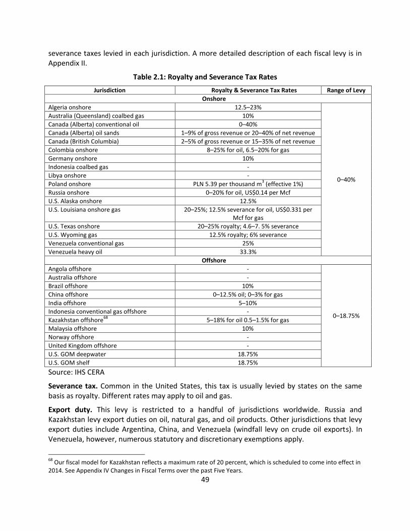
49

severance taxes levied in each jurisdiction. A more detailed description of each fiscal levy is in Appendix II.

Table 2.1: Royalty and Severance Tax Rates

Jurisdiction Royalty & Severance Tax Rates Range of Levy

Onshore

Algeria onshore 12.5–23%

0–40%

Australia (Queensland) coalbed gas 10%

Canada (Alberta) conventional oil 0–40%

Canada (Alberta) oil sands 1–9% of gross revenue or 20–40% of net revenue

Canada (British Columbia) 2–5% of gross revenue or 15–35% of net revenue

Colombia onshore 8–25% for oil, 6.5–20% for gas

Germany onshore 10%

Indonesia coalbed gas -

Libya onshore -

Poland onshore PLN 5.39 per thousand m3 (effective 1%)

Russia onshore 0–20% for oil, US$0.14 per Mcf

U.S. Alaska onshore 12.5%

U.S. Louisiana onshore gas 20–25%; 12.5% severance for oil, US$0.331 per Mcf for gas

U.S. Texas onshore 20–25% royalty; 4.6–7. 5% severance

U.S. Wyoming gas 12.5% royalty; 6% severance

Venezuela conventional gas 25%

Venezuela heavy oil 33.3%

Offshore

Angola offshore -

0–18.75%

Australia offshore -

Brazil offshore 10%

China offshore 0–12.5% oil; 0–3% for gas

India offshore 5–10%

Indonesia conventional gas offshore -

Kazakhstan offshore68

5–18% for oil 0.5–1.5% for gas

Malaysia offshore 10%

Norway offshore -

United Kingdom offshore -

U.S. GOM deepwater 18.75%

U.S. GOM shelf 18.75%

Source: IHS CERA

Severance tax. Common in the United States, this tax is usually levied by states on the same basis as royalty. Different rates may apply to oil and gas.

Export duty. This levy is restricted to a handful of jurisdictions worldwide. Russia and Kazakhstan levy export duties on oil, natural gas, and oil products. Other jurisdictions that levy export duties include Argentina, China, and Venezuela (windfall levy on crude oil exports). In Venezuela, however, numerous statutory and discretionary exemptions apply.

68

Our fiscal model for Kazakhstan reflects a maximum rate of 20 percent, which is scheduled to come into effect in 2014. See Appendix IV Changes in Fiscal Terms over the past Five Years.

50

2.2.2.2 Profit-based Levies

Income tax. This is the most common levy and often not oil industry specific. A few jurisdictions, however, exempt the oil industry from the generally applicable corporate income tax and impose a petroleum income tax. Incentives are often provided in the form of accelerated recovery of development costs, depletion allowances, infrastructure credits, and other benefits. A state income tax may be levied in addition to the federal income tax with appropriate deductions. Table 2.2 contains the range of nominal income tax rates in the 29 jurisdictions covered by this study.

Table 2.2: Range of Income Tax Rates

Jurisdiction Nominal Income Tax Rate Range of Tax

Onshore

Algeria onshore 30%

0–50%

Australia (Queensland) coalbed gas 30%

Canada (Alberta) conventional oil 16.5% federal; 10% provincial

Canada (Alberta) oil sands 16.5% federal; 10% provincial

Canada (British Columbia) 16.5% federal; 11% provincial

Colombia onshore 33%

Germany onshore 15% federal: 14% municipal

Indonesia coalbed gas 40%

Libya onshore -

Poland onshore 19%

Russia onshore 20%

U.S. Alaska onshore 35% federal; 1–9.5% state

U.S. Louisiana onshore gas 35% federal; 8% state

U.S. Texas onshore 35% federal

U.S. Wyoming gas 35% federal

Venezuela conventional gas 34%

Venezuela heavy oil 50%

Offshore

Angola offshore 50%

20–50%

Australia offshore 30%

Brazil offshore 34%

China offshore 25%

India offshore 25%

Indonesia conventional gas offshore 40%

Kazakhstan offshore 20%


Norway offshore 28%

United Kingdom offshore 30%

U.S. GOM deepwater 35%

U.S. GOM shelf 35%

Source: IHS CERA

51

Petroleum profit and windfall taxes. Such taxes are usually levied in addition to income tax and are designed to provide the government with a share of the upside of highly profitable projects. They can be levied on the same basis as income tax with additional credits or allowances, as in the United Kingdom and Norway, or they may be linked to the ratio of cumulative revenue to cumulative expenses, as in Kazakhstan. Quite often such taxes are levied on sliding scales linked to commodity prices, such as the Alaskan Clear and Equitable Share (ACES), Venezuelan Windfall Profits Tax, or China’s Special Revenue Charge. The maximum tax rate can be as high as 75 percent. Table 2.3 shows the range of special petroleum taxes and windfall profits taxes in the 29 jurisdictions covered in this study.

Table 2.3: Range of Special Petroleum Taxes

Jurisdiction Special Petroleum Tax & Windfall Tax Range of Levy

Onshore

Algeria onshore 30–70%

0–75%

Australia (Queensland) coalbed gas -

Canada (Alberta) conventional oil -

Canada (Alberta) oil sands -

Canada (British Columbia) -

Colombia onshore 30–50%

Germany onshore -

Indonesia coalbed gas -

Libya onshore -

Poland onshore -

Russia onshore -

U.S. Alaska onshore 25–75%

U.S. Louisiana onshore gas -

U.S. Texas onshore -

U.S. Wyoming gas -

Venezuela conventional gas -

Venezuela heavy oil 50%

Offshore

Angola offshore -

0–70%

Australia offshore 40%

Brazil offshore 0–40%

China offshore 20-40%

India offshore -

Indonesia conventional gas offshore -

Kazakhstan offshore 0–60%


Norway offshore 50%

United Kingdom offshore 32%

U.S. GOM deepwater -

U.S. GOM shelf -

Source: IHS CERA

52

Profit sharing. A feature of production sharing agreements (PSAs) provides for sharing profits between the host government and investor after recovery of allowable costs. A cost recovery ceiling applies, usually to minimize the government’s revenue risk.69 Profits may be shared on sliding scales based on production volumes, rate of return, or revenue-cost ratio. When designed as a resource rent tax, i.e., profits being shared between the government and the investor after the project has reached a specified rate of return, this levy shifts all the revenue risk to the government. Table 2.4 provides the indicative cost recovery ceilings and range of profit share allocated to the host government under the respective production sharing systems.

Table 2.4: Production Sharing Mechanisms

Jurisdiction Cost Recovery Ceiling Government Profit Share

Angola offshore 50% 30–80% China offshore 65% 51–65.7% India offshore 100% 10–60% Indonesia conventional gas 90% 60–65% Indonesia coalbed gas 80% 55% Libya onshore Equivalent to contractor share 4–85% Malaysia offshore 30–70% 20–90%

Source: IHS CERA

2.2.2.3 Equity Participation

Governments sometimes take a greater risk in upstream oil and gas investment by taking an equity interest. Such participation is motivated by the desire to share in the project upside as well as the nationalistic tendency to exercise greater control over natural resources and facilitate transfer of technology and know-how. Such interest usually falls under two main categories: working interest, whereby the NOC pays up its share right from the start; and carried interest, whereby the investor carries the NOC through exploration and sometimes through development. Usually the government pays its equity share through proceeds from its production participation.70 Table 2.5 shows the range and the type of state participation.

69

The cost recovery limit is an implicit royalty that ensures the government gets a share of the revenue up front. 70

Other less common forms of equity participation include tax swapped for equity, equity in exchange for non-cash contribution, etc, Sunley, Baunsgaard, Simard, Revenue from the Oil and Gas Sector, 9-10.

53

Table 2.5: State Participation

Jurisdiction State Participation Type of Interest Timing of Participation

Onshore

Algeria onshore 51% Carried Discovery


- - -


- - -

Canada (Alberta) oil sands - - -

Canada (British Columbia) - - -

Colombia onshore - - -

Germany onshore - - -

Indonesia coalbed gas - - -

Libya onshore 50% and 85% Carried Discovery (no repayment of past

cost)

Poland onshore - - -

Russia onshore - - -

U.S. Alaska onshore - - -

U.S. Louisiana onshore gas - - -

U.S. Texas onshore - - -

U.S. Wyoming gas - - -

Venezuela conventional gas 35% Carried Discovery

Venezuela heavy oil 60% Working interest Development

Offshore

Angola offshore 20% Carried Discovery

Australia offshore - - -

Brazil offshore 30% Working interest Exploration

China offshore 51% Carried Discovery

India offshore - - -


10% Carried Discovery

Kazakhstan offshore 50% Carried Production

Malaysia offshore 40% Carried Discovery

Norway offshore - - -

United Kingdom offshore - - -

U.S. GOM deepwater - - -

U.S. GOM shelf - - -

Source: IHS CERA

54

2.2.2.4 Quasi-fiscal Instruments

Fiscal systems usually consist of fiscal as well as quasi-fiscal instruments. The most common quasi-fiscal instruments are bonuses, rentals, and training or research fees. Such fees usually provide upfront revenue for the government; however, they may discourage investment in marginal fields. Bonuses may be payable upon execution of a contract or lease (signature bonuses), upon commercial discovery (discovery bonuses), or once production reaches certain volumetric thresholds (production bonuses). From a government perspective, bonus payments are a desirable means of ensuring early revenue. Signature bonuses and rentals are more commonly used than other quasi-fiscal levies. Table 2.6 identifies jurisdictions that provide for various bonus payments.

Table 2.6: Bonus Types

Jurisdiction

Bonus

Training Signature Discovery & Production

Onshore

Algeria onshore √ - -

Australia (Queensland) coalbed gas - - -

Canada (Alberta) conventional oil √ - -

Canada (Alberta) oil sands √ - -

Canada (British Columbia) √ - -

Colombia onshore - - -

Germany onshore - - -

Indonesia coalbed gas √ - -

Libya onshore √ √ √

Poland onshore - √ -

Russia onshore √ - -

U.S. Alaska onshore √ - -

U.S. Louisiana onshore gas √ - -

U.S. Texas onshore √ - -

U.S. Wyoming gas √ - -

Venezuela conventional gas √ - -

Venezuela heavy oil √ - -

Offshore

Angola offshore √ - √

Australia offshore - - -

Brazil offshore √ - -

China offshore √ - -

India offshore - - -

Indonesia conventional gas offshore √ - -

Kazakhstan offshore71

√ √ -

Malaysia offshore - √ -

Norway offshore - - -

United Kingdom offshore - - -

U.S. GOM deepwater √ - -

U.S. GOM shelf √ - -

Source: IHS CERA

71

Our fiscal model for Kazakhstan reflects a maximum rate of 20 percent, which is scheduled to come into effect in 2014. See Appendix IV Changes in Fiscal Terms over the past Five Years.

55

2.2.3 Limitations of Government Take

As a statistic, the government take information is as reliable as the information it is based upon. Therefore, it is important that those who use government take as an input in analysis understand the approach taken and the assumptions that were made. Since the only reliable way to calculate government take is after a project is completed, provided that there is access to all the historical costs and revenue information related to that project, any government take calculation should be qualified by the assumptions made. 72

Several oil and gas fiscal systems apply within each jurisdiction. Understanding which fiscal system is selected is also important. Most countries award contracts based on negotiated agreements. A model contract often serves as the basis for negotiation; however, fiscal terms are usually negotiable and will depend on the perceived prospectivity, commodity prices, and the bargaining power of the parties at the time the contract is negotiated. Thus, a statement that the government take in a particular jurisdiction is X or Y percent is an oversimplification. Even in countries where the fiscal terms are prescribed by law, there are several fiscal systems in place depending on the time the license was awarded. Therefore, it is important to understand which fiscal system within the respective jurisdiction is being analyzed, since the government take will vary with each fiscal system.

Even within the same fiscal system, government take varies with commodity prices, finding and development costs, reserve size, reservoir characteristics, distance from infrastructure, water depth, and other factors. As the analysis shows, government take varies with project profitability. Under fiscal systems that apply ad valorem levies, such as royalties or severance taxes similar to those that apply in the United States, the government take can reach as high as 99 percent when the profits are marginal. It is important to understand whether these results are included or excluded from the calculation of the average or range of government take. Although an argument can be made that such projects will probably not proceed with development and therefore should not be taken into account in the analysis, the counterargument would be that even the projects that appear highly profitable at the planning stage could turn into marginal ones, as a result of drastic market changes, cost overruns, regulatory delays, human error, and other developments.73 Given that sunk costs are never taken into account in projecting future cash flows, these projects are rarely abandoned. Yet they are often excluded from the government take statistic.

The government take statistic accounts for the share of revenue accruing to the government over the full project cycle, i.e., from award of license or contract to decommissioning and abandonment. Although the cash flow is generated on an annual basis, the government take statistic per se does not reveal the timing of revenue and the sharing of risk between the investor and the government. Thus, a government take statistic of 90 percent under a production sharing system does not explain whether the government revenue is front-end loaded or back-end loaded, or whether the government shares the risk by investing through the

72

Kaiser and Pulsipher, Fiscal System Analysis, 9. 73

“A ‘tough’ contract may be highly profitable, while a very ‘favorable’ contract may not be. Good geologic projects

do not always translate to profitable ventures.” Kaiser and Pulsipher, Fiscal System Analysis,10.

56

NOC, and more importantly fails to explain why a project that does not yield positive rates of return to investors under a fiscal system reported to have a 55–65 percent government take could generate positive returns under a fiscal system with 90 percent government take.

Regardless of the approach taken, all studies involving government take, including this one, are based on a set of assumptions with respect to capital and operating cost, commodity price, reserve size, and other inputs. In real life, projects that yield a high government take in studies like this one could in fact generate less revenue to the government over the life of the project than projects of similar reserve size and market conditions in a jurisdiction with a lower government take statistic. Thus, under a fiscal system that does not provide for equitable sharing of the project upside between the host government and the investor, there is less incentive to increase project profitability. In such cases the revenue accruing to the host government could be lower than projected under hypothetical analysis. Since data related to project historical costs and revenue are not publicly available, there is no accurate way of determining who the actual winners or losers are in this race to the top.

2.3 Literature Review

In 2008 the GAO published Oil and Gas Royalties: The Federal System for Collecting Oil and Gas Revenues Needs Comprehensive Reassessment.74 The report made a finding that the GOM has a relatively low government take. At the time the GAO report was published, royalty rates in the GOM were changed twice. First, in 2007, the 12.5 percent rate applicable to acreage in water depths of 400 meters and deeper was changed to 16.67 percent, the same as the rate that applied to shallow-water acreage. Then, in 2008, the royalty rate for shallow and deepwater acreage was increased to 18.75 percent. However, the studies the GAO reviewed predated the royalty changes and did not reflect the current fiscal systems in the GOM. Although the GAO study does not distinguish between the two fiscal systems applicable in the GOM (despite the significant differences between the two at the time the study was written), from the data that GAO is quoting we have been able to ascertain that it was referring to the deepwater GOM fiscal system. Since one of the alternative fiscal systems proposed for this study consists of a 12.5 percent royalty rate, the rate applicable in the deepwater GOM at the time the report was written, we have used the economic analysis generated for that purpose to review the findings of the GAO.

2.3.1 Government Take Referenced by GAO

The results of our economic analysis, based on modeling 20 actual discoveries made in the GOM during the past ten years, show that at a royalty rate of 12.5 percent, the government take statistic ranges between 47 and 74 percent in deepwater projects and between 49 and 76 percent on the shelf under our low, base, and high price and cost scenarios of $45, $75, and $105 per barrel for crude oil and $4, $6 and $8 per Mcf for natural gas.75

74

GAO, Oil and Gas Royalties, 6. 75

These ranges exclude the cases where the government take reaches 100 percent. See Appendix III for results of individual cases under all three price and cost scenarios.

57

The data quoted by the GAO, including a presentation by IHS CERA, show the following government take statistics:

Table 2.7: Studies Referenced by GAO

Study Rank of GOM

Government Take

Percentage of Government Take

Highest Lowest GOM

OUR FAIR SHARE, Report of the Alberta Royalty Review Panel, Sept. 18, 2007 (analysis done by the Alberta Department of Energy).

16/19 77.00% 39.00% 49.00%

Cambridge Energy Research Associates: 2002 vs. 2007.

17/17 95.00% 49.00% 49.00%

Van Meurs Corporation: “Comparative Analysis of Fiscal Terms for Alberta Oil Sands and International Heavy and Conventional Oils,” May 17, 2007.

25/28 92.00% 29.05% 47.00%

Wood Mackenzie: “Government Take: Comparing the Attractiveness and Stability of Global Fiscal Systems,” Wood Mackenzie, June 2007.

93/104 98.04% 18.50% 44.09%

Source: GAO 2008.

Our economic analysis supports the argument that the government take varies with commodity prices, finding and development costs, reserve size, reservoir characteristics, distance from infrastructure, water depth, and other factors. There is no single government take statistic, unless the system is absolutely neutral. The wide ranges of government take from 47 percent for profitable projects to 74 percent for marginal ones in the deepwater GOM suggest a highly regressive fiscal system that penalizes marginal fields.76

Understanding the assumptions made and the fiscal system used is very important in deciding the usefulness of the analysis coming from other studies. With respect to IHS CERA’s presentation showing a 49 percent government take, that presentation was not prepared to show the range of government take in each jurisdiction but rather to illustrate the degree of change in government take as a result of changing fiscal policies in various jurisdictions, and it relied on applying a single model for each fiscal system. It was designed to measure the degree of change in government take for projects yielding a specific rate of return rather than to compare jurisdictions and assess their relative competitiveness. A similar chart (Figure 6.1) has been produced for this study in the analysis of fiscal stability.

The study by Van Meurs Corporation referenced in the GAO report does in fact represent a wider range of the U.S. GOM government take between 47 and 56 percent. That is perhaps

76

Under a regressive fiscal regime such as the U.S. federal fiscal systems, the government take declines as project profitability increases and increases as profitability declines. Such systems increase the marginal cost of development and often deter the development of marginal fields.

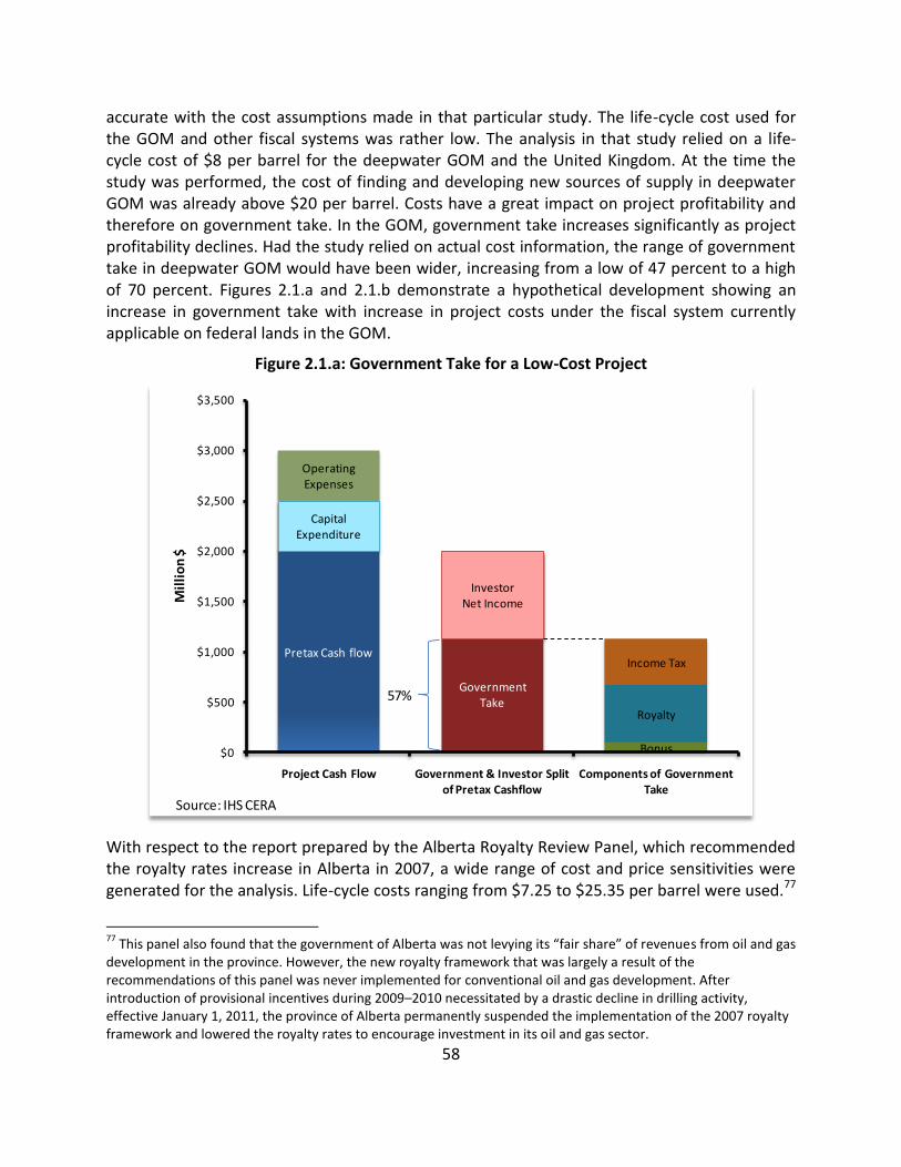
58

accurate with the cost assumptions made in that particular study. The life-cycle cost used for the GOM and other fiscal systems was rather low. The analysis in that study relied on a life-cycle cost of $8 per barrel for the deepwater GOM and the United Kingdom. At the time the study was performed, the cost of finding and developing new sources of supply in deepwater GOM was already above $20 per barrel. Costs have a great impact on project profitability and therefore on government take. In the GOM, government take increases significantly as project profitability declines. Had the study relied on actual cost information, the range of government take in deepwater GOM would have been wider, increasing from a low of 47 percent to a high of 70 percent. Figures 2.1.a and 2.1.b demonstrate a hypothetical development showing an increase in government take with increase in project costs under the fiscal system currently applicable on federal lands in the GOM.

Figure 2.1.a: Government Take for a Low-Cost Project

Pretax Cash flow

Government Take

Bonus

Royalty

Income Tax

Investor Net Income

Capital Expenditure

Operating Expenses

$0

$500

$1,000

$1,500

$2,000

$2,500

$3,000

$3,500

Project Cash Flow Government & Investor Split of Pretax Cashflow

Components of Government Take

Mil

lio

n $

57%

Source: IHS CERA

With respect to the report prepared by the Alberta Royalty Review Panel, which recommended the royalty rates increase in Alberta in 2007, a wide range of cost and price sensitivities were generated for the analysis. Life-cycle costs ranging from $7.25 to $25.35 per barrel were used.77

77

This panel also found that the government of Alberta was not levying its “fair share” of revenues from oil and gas development in the province. However, the new royalty framework that was largely a result of the recommendations of this panel was never implemented for conventional oil and gas development. After introduction of provisional incentives during 2009–2010 necessitated by a drastic decline in drilling activity, effective January 1, 2011, the province of Alberta permanently suspended the implementation of the 2007 royalty framework and lowered the royalty rates to encourage investment in its oil and gas sector.

59

Appendices attached to the report showed that for life-cycle costs of $21.73 per barrel and $25.35 per barrel, which would be representative of costs for deepwater GOM at the time of the report, government take ranged between 47 and 63 percent. The data from the same study indicate that at the cost levels mentioned above, average rates of return are achieved in the GOM only when crude oil prices are between $60 and $90 per barrel, based on the analysis of the authors.78 Similar conclusions can be drawn with respect to profit-to-investment ratio, an indicator often used by companies when making investment decisions. According to the Alberta Royalty Review study average profit-to-investment ratios at 10 percent discount were reached when crude oil prices were between $70 and $120 per barrel for projects with life-cycle costs of $21.73 and $25.35 per barrel.

Figure 2.1.b: Government Take for a High-Cost Project

Pretax Cash flow Government Take

Bonus

Royalty

Income Tax

Investor Income

Capital Expenditure

Operating Expenses

$0

$500

$1,000

$1,500

$2,000

$2,500

$3,000

$3,500

Project Cash Flow Government & Investor Split of Pretax Cashflow

Components of Government Take

Mil

lio

n $

78%

Source: IHS CERA

Despite the shortcoming of using the same field development model to compare various jurisdictions, for example not taking into account the difference in timing when bringing onstream an onshore field as opposed to an offshore field, well productivity, or typical field sizes expected in each jurisdiction, the Alberta Royalty Review study, though it may support the finding that the government take was lower than average in the GOM, also indicates that average rates of return are reached when prices are above $70 per barrel. In determining the competitive position of a particular oil and gas jurisdiction, it is important to consider

78

The Alberta Royalty Review study considers average rates of return to range between 12 and 17 percent.

60

profitability indicators, an approach that was followed by the Alberta Royalty Review Panel.

The GAO recognizes the shortcomings of the government take statistic, yet it does not consider other indicators often used to make investment decisions. the GOM is an attractive investment environment; however, it is also among the most expensive next to Alaska and other arctic environments. As exploration and production move beyond 5,000 feet, which seems to be the area with the greatest growth potential in the GOM according to data from the EIA and the DOI, achieving desirable rates of return is going to be quite challenging.

The GAO report made no findings with respect to federal onshore jurisdictions. A recent article published in the Oil and Gas Journal described the government take on federal lands onshore as ranging between 61.8 and 74.2 percent.79 Despite the shortcoming of using the same production, cost, and prices for each fiscal system, the article supports a finding of high government take in both federal and state lands in the United States.80 The economic models generated for our study resulted in government take ranges between 54 and 93 percent for Wyoming natural gas fiscal system, with a 66 percent jurisdictional average.

A recent study commissioned by the government of Alberta to examine its competitive position, instigated by drastic decline in drilling activity between 2007 and 2009, incorporated onshore U.S. jurisdictions in the analysis, including Wyoming.81 Although the study did not display the data separately for each U.S. jurisdiction, it made, among others, two general observations relevant to this study:

The investment attractiveness of conventional wells in the United States is generally not as attractive as that for U.S. shale gas wells.

On average, conventional wells in the United States and Canada were generally found to be marginally economic under anticipated price conditions.82

2.3.2 The Government Take for New Acreage

The currently applicable royalty rate of 18.75 percent in the GOM has significantly increased government take compared with the rates referenced by the GAO report. For shelf projects modeled for this study, the range of government take varies from 57 to 99 percent, with a fiscal system average of 79 percent.83 For the deepwater GOM the results of the study show that government take ranges from 53 to 90 percent, with a fiscal system average of 64 percent. Even though the current GOM shelf and deepwater fiscal systems are almost identical—the only difference lies in rental rates, which are usually a rather minor component of government take

79

Jerry Kepes, Barry Rogers, and Pedro van Meurs, “Gas Prices, Other Factors Indicate Changes in North American

Shale Play Fiscal Systems,” Oil and Gas Journal 109, (2011). 80

Ibid. The article states that the average government take on state lands in the United States ranges between 62.5 and 77.3 percent. 81

Sierra Systems, Appendix B-12. 82

This helped avoid concentrating on the lesser important differences among states and facilitated comment on

whether there is a fundamental difference in economic attractiveness between the United States and Canada. 83

In calculating averages, IHS CERA has eliminated projects that result in 100 percent government take under all three price and cost scenarios. For a detailed description of the approach, see Appendix III.

61

and rarely have a noticeable impact on the overall government take percentage—the average government take varies significantly between them. The relatively small size of the recent discoveries on the shelf leads to a higher per-unit cost compared with the deepwater projects. This ultimately has an impact on the government take. Although this study shows that the U.S. government collects less revenue on a per-project basis from new discoveries on the shelf, the government take statistic tells a different story. For this reason, and others, government take reveals only part of the full picture.

In 2008 the GAO concluded that the U.S. government was losing billions of dollars in revenue. This finding was based on the fact that the U.S. GOM government take ranked lower than that in most jurisdictions, i.e., 93 out of 104 fiscal systems. However, a high government take statistic does not always mean high revenues or realization of that particular statistic. Table 2.8 shows that the majority of the fiscal systems having a higher average government take than the three federal fiscal systems rely more heavily or entirely on profit-based sliding scale levies. Such levies are usually structured with a lower share to the government when profits are low, with the government share progressively increasing as profitability increases. In the majority of the profit-based fiscal systems, the government’s ability to capture the upside and to fully realize the take stated in studies such as this one depends largely on the profits realized. Given that these progressive levies encourage tax avoidance or inefficient development of the resource, it is quite possible that in real life revenue accruing to the government may not be as high as expected by a government take study.84 Despite the theoretical appeal, resource rent taxes and profit-sharing mechanisms designed to mirror the resource rent tax have not been a significant revenue raiser in practice.85

84

Over the past decade, capital and operating costs in the oil and gas upstream sector have more than doubled. This cost escalation ultimately shrinks the profit available to be shared between the host government and investor. In those instances where the fiscal system relies heavily on progressive profit-based levies, this increase in cost could contribute to keeping the government profit share to the lower thresholds, thus never realizing the full potential of the fiscal system as displayed in studies offering a benchmarking of fiscal terms. 85

Sunley, Baunsgaard, Simard, Revenue from the Oil and Gas Sector, 6; Allan L. Clark, “Resource Rent Extraction, Application, Consumption, Investment and Sustainability of Resource-Based Development in Resource-Rich Island Economies,”presented at UNCTAD Regional Workshop on the Constraints, Challenges, and Prospects for the Commodity-Based Development and Diversification in the Pacific Island Economies on August 18–20, 2001. The U.S. government adopted, on an experimental basis, net profit sharing between 1980 and 1982. The reasoning behind the move was that it would eliminate distortive royalties and extract larger payments during the production stage. The experiment was considered a failure and ended in 1982. See James L. Smith, Daniel R. Siegel, and C. S. Agnes Cheng, 1988. “Failure of the Net Profit Share Leasing Experiment for Offshore Petroleum Resources,” The Review of Economics and Statistics 70, no. 2 (MIT Press: May 1988), 199-206. For issues related to resource rent taxation, see Ross Garnaut, “Principles and Practice of Resource Rent Taxation,” Australian Economic Review 43, no. 4 (2010), 347–356. The author argues that the various means of taxing resource rents in practice either fall short of the ideal of neutrality or collect only a small proportion of the mineral rent.

62

Table 2.8: Reliance on Profit-Based Levies

Fiscal System Average Government

Take Reliance on Profit-based Levies

Venezuela heavy oil 95% Medium

Malaysia offshore 93% High

Libya onshore 91% High

Angola offshore 90% High

Algeria onshore 86% High

U.S. Louisiana onshore 85% Low

Venezuela conventional gas 84% Low

Indonesia conventional gas offshore 82% High

Colombia onshore 82% High

China offshore 80% High

Indonesia coalbed gas 79% High

U.S. GOM shelf 79% Low

Kazakhstan offshore 78% High

U.S. Alaska onshore 76% High

U.S. Texas onshore 76% Low

Norway offshore 73% Total

Russia onshore 73% Low

Brazil offshore 72% Low

Australia offshore 71% Total

Canada (Alberta) oil sands 67% High

U.S. Wyoming onshore 66% Low

U.S. GOM deepwater 64% Low

United Kingdom 62% Total

Germany onshore 61% Low

Canada (Alberta) conventional oil 59% Low

India offshore 57% High

Australia (Queensland) coalbed gas 40% High

Canada (British Columbia) 39% High

Poland onshore 28% Medium

Source: IHS CERA

The GAO report concludes that the federal government lost billions of dollars in forgone revenue because the royalty system had no built-in flexibility to adjust the rate as the market changed. An assessment of whether the government actually gained or lost revenue from a specific action or inaction cannot be made from studies comparing fiscal terms such as the ones quoted by the GAO or this particular study. This type of analysis is usually done through long-term forecasts of the exploration and production activity of the respective jurisdiction, the expected revenue from the alternative policy decisions, and the potential offsets associated with each alternative. A recent study commissioned by the BOEM titled “Policies to Affect the

63

Pace of Leasing and Revenues in the Gulf of Mexico” reviewed among others the sliding scale royalty alternative ranging between 12.5 and 35 percent as well as an increased 35 percent flat royalty alternative.86 This study, which was conducted by Economic Analysis Inc. and Marine Policy Center, focused on tracts to be leased on the central and western GOM planning areas over the 50-year period from 2010 to 2060. Tables 2.9 and 2.10 contain the assessment criteria used by the study “Policies to Affect the Pace of Leasing and Revenues in the Gulf of Mexico” measured against the OCS Lands Act goal of expeditious and orderly development of the OCS resources and the goal to obtain a fair market value for leased resources.87

The study concluded that any potential gains from higher royalty rates are offset by “associated reductions in cash bonus bids, area rental fees, and federal corporate taxes.” The study also concluded that higher royalty rates would adversely affect expeditious development of Outer Continental Shelf resources. With respect to coastal states, the study found that any state gains due to higher royalty revenue are likely to be offset by reduced onshore spending associated with lower levels of offshore activities. When comparing the sliding scale royalty to the status quo (the current fiscal system with 18.75 percent royalty), the study conducted by Economic Analysis Inc. and Marine Policy Center found that the application of this alternative would result in a 13 percent reduction of total production from the central and western GOM planning areas and a 1 percent decline in total discounted revenues to the federal government.

2.3.3 Fair Share

One of the policy objectives of the OCS Lands Act is to assure receipt of fair market value for the lands leased and rights conveyed by the federal government. The Mineral Leasing Act, which governs the oil and gas activities onshore, authorizes the Secretary of the Interior to set the minimum bid so as to enhance financial returns to the United States. To fulfill the mandate of the OCS Lands Act, BOEM follows specific bid adequacy procedures to ensure that the government receives fair market value for the offshore tracts receiving bids.88

86

J. James Opaluch, et al., “Policies to Affect the Pace of Leasing and Revenues in the Gulf of Mexico,” U.S.

Department of the Interior, Bureau of Ocean Energy Management, Regulation and Enforcement, Gulf of Mexico OCS Region, New Orleans, LA. OCS Study BOEMRE 2011-014 (November 2010), 160. 87

The study considered 12 alternatives; however, for the purpose of this section we focus on just two: the sliding scale royalty and the increased royalty. 88

This process is carried out in several phases and incorporates geological and geophysical data along with reserve, resource, engineering, and economic information into a sophisticated discounted cash flow computer model. The goal of that model is to achieve estimates of fair market value on tracts receiving bids.

64

Table 2.9: Impact of Royalty Alternatives on Exploration and Production Activity in the Gulf of Mexico

Goal: Expeditious and Orderly Development of OCS Resources

Criteria Current Leasing System

Sliding Scale Royalty (12.5–35%)

Increase Royalty to 35%

Sliding Scale—Change from Status Quo

Royalty Increase—Change from Status Quo

Percent Change—Sliding Scale

Percent Change—Increased Royalty

Total production (MMboe 22,113 19,131 17,251 (2,982) (4,862) -13% -22%

Discounted production (MMboe) 3,733 3,199 2,907 (534) (826) -14% -22%

Fields discovered 954 952 936 (2) (18) 0% -2%

Exploration wells 10,931 10,866 10,412 (65) (519) -1% -5%

Development wells 5,267 4,638 4,219 (629) (1,048) -12% -20%

Production wells 11,467 10,288 9,487 (1,179) (1,980) -10% -17%

Average annual number of tracts offered 5,598 5,598 5,598 — — 0% 0%

Average annual tracts sold 119 119 118 — (1) 0% -1%

Source: Economic Analysis Inc. and Marine Policy Center

Table 2.10: Impact of Royalty Alternatives on Federal Government Revenue from the Gulf of Mexico

Goal: Obtain Fair Market Value for Leased Resources

Criteria Current Leasing System

Sliding Scale Royalty (12.5–35%)

Increase Royalty to 35%

Sliding Scale—Change from Status Quo

Royalty Increase—Change from Status Quo

Percent Change—Sliding Scale

Percent Change—Increased Royalty

Discounted high bids $31,464 $26,211 $19,278 ($5,253) ($12,186) -17% -39%

Discounted royalties $44,290 $53,079 $67,804 $8,789 $23,514 20% 53%

Discounted area rental payments $5,579 $5,574 $5,537 ($5) ($42) 0% -1%

Total discounted OCS revenues $81,333 $84,863 $92,619 $3,530 $11,286 4% 14%

Discounted federal taxes $24,541 $20,465 $15,756 ($4,076) ($8,785) -17% -36%

Total discounted revenues $105,874 $105,328 $108,374 ($546) $2,500 -1% 2%

Source: Economic Analysis Inc. and Marine Policy Center

65

The GAO made a finding that the U.S. government is not receiving a fair return on oil and gas leases in the GOM. That finding, however, appears to be based on a ranking of government take rather than an analysis of the bid adequacy procedures or an accounting of the amounts received via signature bonuses. Based on the ranges of the GOM government take reported by the GAO, we have concluded that the specific GOM government takes did not include signature bonuses or account for exploration risk.89 Studies that factored in risk and present value in the mid-1980s and late-1990s reported the U.S. OCS government take closer to 77 percent.90 If not accounted for in the government take statistic, a significant source of revenue accruing to the U.S. government is being overlooked.91

2.3.4 What Is Fair Share?

All the changes of fiscal terms introduced over the past five years have been based on the premise that the government is not receiving a fair share. Whether the change has been politically motivated, as in the nationalization of Venezuela’s oil industry, or purely for revenue collection purposes, as in Alberta, Alaska, Australia, Newfoundland and Labrador, and elsewhere, the question has always been the same: Is the government getting a fair share of the revenue from its oil and gas resources?

Although there is universal consensus that the government and the public should receive a fair share of the revenue from the oil and gas resources, there appears to be no standard or benchmark as to what that means. “Fair share” is a judgment or opinion that can neither be refuted nor proven.92 The Alberta Department of Energy in its 2007 Royalty Review recognized the inherently subjective nature of the fair share concept.93 Nonetheless, it concluded that Alberta was not receiving its fair share but without properly defining the benchmark or justifying the reasoning for such a conclusion. Although the study conducted regional and international comparisons, it did not identify the metrics on which such a finding was based, nor did it identify what target the government take should reach for it to be considered fair. In fact, similar to the GAO finding, the reasoning was related to the fact that the royalty rates and formulas had not kept pace with changes in resource base, energy markets, and conditions in other energy-rich jurisdictions. Basically, fairness was judged on the basis that royalties had not changed for a long time rather than considering the fiscal system as a whole, including that the conventional resources had reached maturity or that Alberta’s royalty rates were already among the highest in the world. To achieve a fair return the study recommended “an equitable and flexible administrative framework that maintains Alberta’s competitive edge for energy investment.”94 Less than two years later, the Government of Alberta reversed the royalty

89

In a phone interview with a GAO staff member in 2007, IHS CERA pointed out that the government take presented in that particular graph did not account for signature bonuses. 90

Daniel Johnston, “Changing Fiscal Landscape,” Journal of World Energy Law and Business 1, 1 no. 1 (2008).

91 Ibid. See also Andrew Derman and Daniel Johnston, “Bonuses Enhance Upstream Fiscal System Analysis,” Oil and

Gas Journal 51, February 8, 1999,5. 92

Locke, Is Newfoundland and Labrador Getting Its Fair Share? 93

Alberta Department of Energy, Royalty Information Briefing # 2, 1. 94

Alberta Department of Energy, Royalty Information Briefing # 2, 1

66

framework in order to maintain a competitive edge.95

Similar approaches were followed by other governments that attempted a benchmarking of fiscal terms to justify an increase in the government take. Alaska under Governor Sarah Palin conducted hearings before the introduction of the petroleum profits tax. In fact, the tax itself was called Alaska Clear and Equitable Share (ACES). At the time of the ACES hearings, Alaska had just introduced a petroleum profits tax (PPT). It is not clear what standard was used for abolishing the newly introduced PPT, which had only been in effect for six months, and for introducing ACES.

Although concerns as to whether the government is receiving a fair share of the oil and gas revenues may be more justified in a fiscal system where all components of the take are fixed, with fiscal systems relying on cash bonus bids for allocation of acreage, such as the federal oil and gas fiscal systems, the bonus bids create a self-correcting mechanism within the overall fiscal system.96 The stakeholders interviewed by the project committee conducting Alberta’s Natural Gas and Conventional Oil Investment Competitiveness study emphasized that in addition to being an objective and fair way to allocate land, the bonus bids also create a potential for a self-correcting mechanism within the fiscal system. Since the bid value represents the economic rent the investors expect to receive from developing the resource, the investors can, within tolerable limits, reduce the amount of the bid if it is felt that the royalty or the government take is too high; likewise, investors may increase the bid amount under conditions where low royalties leave more room for investors.97 Theoretically, pure bonus bidding approximates the optimum allocation mechanism when the government’s objective is to maximize rent capture.98

Bonus bids in the U.S. OCS have acted as self-correcting mechanisms within the federal fiscal systems. During 2005–2010 revenue collected by the DOI from signature bonuses for the U.S. offshore constituted 27 percent of total revenue the DOI collected from offshore oil and gas leases. When each year is examined separately, there is clear evidence that in times of high prices investors have been willing to contribute a significant amount in signature bonuses.99 In 2008, when the oil price reached its highest, at $147 per barrel, revenue from signature bonuses made up 53 percent of the total revenue collected by the DOI from OCS oil and gas leases. The $9 billion collected in signature bonuses alone far outweighed any hypothetical loss in royalty revenue because of a failure to introduce a sliding scale royalty to capture the upside.100 Figures 2.2.a and 2.2.b give a breakdown of the DOI revenue from OCS oil and gas leases and the GOM for the 2005-2010 fiscal years. 101,102

95

Government of Alberta, Energizing Investment. 96



Tordo, Johnston, and Johnston, Countries’ Experience with the Allocation of Petroleum Exploration and Production Rights,18. 99

While the DOI does not rely on bonuses as a "self-correcting mechanism," but as a reflection of past choices on risk sharing, signature bonuses, have in fact acted as a self correcting mechanism for Gulf of Mexico. 100

Given the time lag from award of acreage to first production (five to ten years), the U.S. government would not have been able to reap the benefits of any royalty revisions, even if such revisions were introduced in 2005. 101

There is a discrepancy between the BOEMRE-reported bonuses from lease sales and the Office of Natural

67

Figure 2.2.a: DOI OCS Revenue (Fiscal Years 2005–2010)

$0

$2,000

$4,000

$6,000

$8,000

$10,000

$12,000

$14,000

$16,000

$18,000

$20,000

2005 2006 2007 2008 2009 2010

Mil

lio

n D

oll

ars

Fiscal Year

Bonus

Rents

Royalty


Federal government revenue from onshore acreage in Wyoming shows a similar trend as the revenue from outer continental shelf acreage. Data on revenue collected in terms of signature bonuses, royalties, and rentals in federal lands in Wyoming shows a 100 percent increase in revenue in 2008 from 2007 (Figure 2.3). However signature bonuses were not the source of additional revenue in times of high commodity prices. The adjusting mechanism in the case of Wyoming was investment in producing capacity. The relative ease with which new sources of supply are brought onstream onshore in the United States compared with offshore acreage led to increased investment in production capacity. Whereas sales volumes of crude oil in Wyoming federal lands continued their steady decline despite the high commodity prices, sales volumes of processed residue gas increased 80 percent in 2008 compared to 2007.103 In 2010 as natural gas prices dropped to $4 Mcf from an average of $8 per Mcf in 2008, the sales volumes of processed residue gas dropped by 52 percent compared with 2008.104 This behavior is supported by the results of the economic analysis conducted for this study, which shows

Resources Revenue because the latter report payments as received, whereas data from the BOEM website is reported when the lease sale occurred. Thus some of the bonus payments pledged in the 2007 lease sales were actually made in 2008. 102

This IHS CERA study refers to the area up to 200 meter water depth as shelf rather than 1,000 feet, since a separate fiscal system can be established for areas in less than 200 meter water depth. 103

According to data from ONRR website sales volumes of crude oil produced from federal lands in Wyoming dropped from 29,844,078 barrels in 2007 to 28,556,565 in 2008, while sales volumes for processed residual gas increased from 547,765,513 Mcf to 998,826,124 Mcf during the same period. 104

According to data from ONRR website sales of processed residue gas in 2010 dropped to 522,711,425 Mcf, lower than the 2007 sales volume of 547,765,513 Mcf.

68

positive rates of return for only one out of five conventional gas fields selected from the pool of discoveries made in the past ten years.

Figure 2.2.b: GOM Bonus Payments (Fiscal Years 2005–2010)

2006 2007 2008 2009 2010

Mil

lio

n U

S D

oll

ars

Year

Deepwater Shelf

Source: BOEMRE

Figure 2.3: DOI Wyoming Revenue (Fiscal Years 2006–2010)

$0

$200

$400

$600

$800

$1,000

$1,200

$1,400

$1,600

2006 2007 2008 2009 2010

Mill

ion

Do

llars

Fiscal Year

Bonus

Rents

Royalty


69

2.4 Features of U.S. Federal Oil and Gas Fiscal Systems

Rights on OCS areas in the United States are awarded through competitive bids under the 1953 OCS Lands Act. Various bidding systems have been prescribed by the Act that differ with respect to the bidding terms or bidding variables. The cash bonus bid with a minimum of 12.5 percent royalty and royalty suspension areas has been the preferred system for awarding acreage in the GOM since 1983. The main elements of the U.S. offshore fiscal systems are signature bonuses, rentals, royalties, and federal income tax (see Table 2.3). The fiscal systems analyzed in this study are those implemented in the recent lease sales in the GOM, which result in different fiscal systems for shelf and for deepwater areas. The only difference between the two fiscal systems lies in the amount of rental payable and minimum signature bonuses.

The Mineral Leasing Act of 1920 governs the management of oil and gas development activities on over 570 million acres of BLM lands and other federal lands as well as on private lands where mineral rights have been retained by the federal government. Section 32 of the Act recognizes the right of the states to levy and collect taxes on improvements, output of mines, or other rights, or assets of any lessee of the United States. Although the levies of the federal government are uniform among all federal lands onshore, the application of Section 32 of the Act results in separate fiscal systems for each state where the federal government administers oil and gas leases.

Table 2.11: Gulf of Mexico Federal Fiscal Systems

Water Depth (meters)

Signature Bonus Rental Royalty

Rate Federal Income

Tax Rate Year Rate

GOM Shelf

<200

Biddable (minimum $25 per

acre)

1–5 $7 per acre

18.75% 35% 6 $14 per acre

7 $21 per acre

8+ $28 per acre

GOM Deepwater

200–400

Biddable (minimum $25 per

acre)

1-5 $11 per acre

18.75% 35%

6 $22 per acre

7 $33 per acre

8+ $44 per acre

400+ Biddable

(minimum $37.50 per acre)

1–5 $11 per acre

6+ $16 per acre

Source: IHS CERA

Onshore acreage is offered under competitive bids; however, parcels that do not receive any competitive bids are available for noncompetitive offers beginning the first business day following the day of the sale. If not withdrawn, these parcels are available for noncompetitive offers for a period of two years following the day of the sale. Table 2.4 summarizes the fiscal system that applies to federal lands within the state of Wyoming, which have been modeled for this study.105

105

Noncompetitive bids are not subject to bonus payments. All other fiscal terms remain unchanged.

70

Table 2.12: Wyoming Federal Fiscal System

Bonus

Rental

Royalty Federal Income Tax

Severance Tax

Ad Valorem (Property Tax)

Conservation Tax Year Rate

Minimum $2/acre

1–5 $1.5/acre 12.5% 35% 6% 6.2%106 0.04%

6–10107 $2/acre

Source: IHS CERA

106

Ad valorem taxes in Wyoming vary by county and range between 6 and 7.3 percent. The 6.2 percent used in this study is the statewide mineral tax district average. 107

The $2 per acre rental is for the remainder of the first term of the lease or until production starts, whichever occurs earlier.

71

3. FACTORS INFLUENCING GOVERNMENT TAKE AND INVESTMENT DECISIONS

3.1 Resource Endowment

Resource endowment, along with the design of the fiscal system, is one of the main factors influencing investment decisions. As a general trend, countries with high prospectivity, low development costs, and a stable investment environment should be able to demand higher levels of government take. Perceived endowment motivates companies to invest in a particular jurisdiction despite high levels of political risk or high levels of government take. What drives fiscal policy is often the government’s perception of its own endowment. Governments that have an unrealistic perception of their endowment often design fiscal policies that fail to attract investment.108 More than 150 jurisdictions have a petroleum fiscal system in place, although fewer than half of them have any significant production.109 Yet some of the toughest fiscal terms are found in jurisdictions with no established production. Having a fiscal system in place and demanding a high government take does not always establish a successful policy. For any ranking or competitiveness review to be meaningful, it is important to find the right peer group.

For each petroleum jurisdiction in this study, we analyzed the exploration and production activity of the past five years and ranked the respective jurisdictions based on production and E&P activity levels as well as exploration success. The deepwater Gulf of Mexico and Texas ranked in the top 30 percent of the selected peer group. However, the other two federal oil and gas jurisdictions, the GOM shelf and Wyoming, ranked in the bottom 20 percent together with Louisiana and Alaska. Figure 3.1 shows the E&P activity scorecard.

The analysis found that the U.S. jurisdictions in general, except for the deepwater GOM, ranked high with respect to the number of wells drilled; however, the size of the discoveries per new-field wildcat drilled was among the lowest. When drilling for shale is excluded, from the perspective of field sizes, onshore jurisdictions in the United States are not as appealing as most of the countries selected for this study. Although a significant number of wells are drilled in the United States each year, they have very low productivity. Most of the conventional oil and gas fields discovered onshore in the United States are smaller than 1 MMboe. Table 3.2 shoes the field size per new field wildcat in the respective jurisdictions.

108

Boadway and Keen. The authors argued that policy makers are “generally less well-informed of the geological and commercial circumstances at all stages of particular resource projects than are those who undertake the exploration, development and extraction.” 109

Out of 116 countries we examined in the IHS Petroleum PEPS database that had one or more petroleum fiscal systems in place, 30 had no established production; an additional 30 had no significant production that would make them competitors of the United States.

72

Figure 3.1: E&P Activity Scorecard

0.00 0.50 1.00 1.50 2.00 2.50 3.00 3.50

Germany

Poland

U.S. Wyoming

U.S. Alaska

U.S. Louisiana

U.S. GOM shelf

Colombia

Malaysia

Indonesia


Kazakhstan

India

Australia (Queensland)

Canada (Alberta)

Libya

United Kingdom

Algeria

Australia offshore

U.S. GOM deepwater

Norway

U.S. Texas

Angola

China

Venezuela conventional oil and gas

Russia

Brazil

E&P Activity Score

Oil Production

Gas Production

No. of New-field Wildcats

Acreage Leased

No. of Operators

Oil Reserves Added

Gas Reserves Added

Reserves per NFW

Success Rate

High Production LevelsHigh E&P Activity

High Exploration Success

Source: IHS CERA

Upon a closer examination of the lease areas granted by the BLM in Wyoming over the past five years, lease sizes usually varied between 80 and 640 acres, when the standard spacing unit for a natural gas well in the U.S. is 640 acres. Even when lease sizes exceeded these ranges, they were large enough to permit the drilling of two to three wells. Although there may be a market for individuals to take on operations of this size in the United States, the conventional oil and gas onshore opportunities in the United States do not compete in the international market. Therefore, they are not likely to attract the same investors as other onshore jurisdictions outside North America covered in this analysis. Except for one field, our analysis of conventional gas cases onshore in Louisiana and on federal lands in Wyoming indicated that none of these resources can be commercially exploited under the current natural gas prices in the North American market.110

110

The conventional fields modeled for Wyoming were brought onstream between 2000 and 2003. Since then, the capital and operating costs have more than doubled according to IHS CERA’s Capital and Operating Costs Indexes. That is one of the reasons that these fields are not economic in the current environment. Also, it is hard to ascertain whether such fields are in fact yielding desirable returns on investment in real life. Two of the fields have just one well drilled in them, and it is quite possible that these fields are sub economic. Sunk costs are never taken into account in projecting future cash flows. After drilling the first well, it makes more sense to continue to produce and recover as much of the original investment as possible, even if the entire project is not economic. The other fields have seven and four wells, respectively; however, the flow rates are too low.

73

Figure 3.2: Field Sizes per New-field Wildcats

0.00 20.00 40.00 60.00 80.00 100.00 120.00 140.00

U.S. Texas

U.S. Louisiana

U.S. GOM Shelf

U.S. Wyoming

Canada (Alberta)

U.S. Alaska

Poland conventional oil and gas

Australia (Queensland)

Colombia

Indonesia conventional gas

Venezuela heavy oil

Russia

India

United Kingdom

Algeria

Kazakhstan

China

Libya

Malaysia

U.S. GOM deepwater

Norway

Australia offshore

Angola

Brazil

Venezuela gas

Field Size per New Field Wildcat (MMboe)

Source: IHS CERA

When remaining reserves are taken into consideration, all three federal oil and gas jurisdictions ranked relatively low compared with Texas and other international oil and gas jurisdictions. When comparing jurisdictions based on average government take among the cases generated for this study, all three federal jurisdictions are levying a higher government take than other jurisdictions relative to their remaining recoverable reserve ranking. Figure 3.3 shows the ranking of remaining recoverable reserves relative to the government take.

74

Figure 3.3: Government Take Relative to Remaining Recoverable Reserve Ranking

Algeria

Angola

Australia offshore

Brazil China

Colombia

Germany

India

Indonesia

Kazakhstan Libya

Malaysia

Norway

Poland

Russia

United Kingdom

Venezuela heavy oil

U.S. GOM deepwater

U.S. GOM shelf

Louisiana

Texas

Alaska

Wyoming

Alberta oil sands

British Columbia

Queensland

Alberta conventional

Venezuela gas

0.00

0.50

1.00

1.50

2.00

2.50

3.00

3.50

4.00

4.50

5.00

0% 10% 20% 30% 40% 50% 60% 70% 80% 90% 100%

Re

ma

inin

g R

ec

ove

rab

le R

es

erv

e R

ati

ng


3.2 Political and Commercial Risk

Political and commercial risk is a factor that companies consider when making investment decisions. Often such risks are reflected in the cost of doing business in a particular jurisdiction. The degree of political or commercial risk is reflected in risk premiums associated with the leasing of facilities and any infrastructure-related work. From the government take perspective, there is no correlation between political risk and government take. The term political risk reflects the perception of risk by investors and international financial institutions in a particular jurisdiction, not necessarily how a government perceives its own risk. That’s why policies related to natural resources taxation in general and the level of government take in particular do not reflect investors’ perception of political risk of the respective jurisdiction.111

In addition to overall political risks that are not industry specific, in periods of volatile commodity prices, investors face several petroleum industry–specific commercial and regulatory risks. Sometimes these risks can be greater than the overall political risk. Thus, it is not unusual for a petroleum jurisdiction with a low overall political risk to have a high

111

Most jurisdictions that are perceived to have a high political risk, such as Venezuela, Libya, Nigeria, Iraq, and others, also demand high government take.

75

commercial and regulatory petroleum risk. The petroleum commercial and regulatory risks can take the form of threat of adverse contract changes or nationalization, currency repatriation or convertibility restrictions, regulatory risk, and opposition to foreign investment in the oil and gas sector.

Threat of adverse contract changes and nationalization is the greatest risk oil and gas investors face when commodity prices are high. Unlike manufacturing or other industries that operate on annual cycles, investment in the oil and gas sector has long lead times.112 Depending on the size of the investment, it could take eight to ten years before first production comes onstream. The time it takes for companies to recover their investment varies to a large extent with the structure of the fiscal system. In fiscal systems that rely heavily on signature bonuses and royalties, such as the ones common in the United States and Canada, it is usually several years after first production that project cash flow turns positive. It could be 15 to 20 years before payout is reached. A lot happens in this 15–20 year time frame. Commodity prices are often not at the same level as when companies signed the lease or entered into a PSA with the resource owner. Costs also change over time, at times rather dramatically. Although governments are usually well informed about commodity prices, their information about project costs is much more limited. Thus, when the change in fiscal terms is not motivated by nationalistic tendencies but rather is based on the perception that the government is not getting its fair share of revenues, access to information about one variable (price) and lack of information about the other important variable (cost) increase significantly the risk that investors take when they sign an oil and gas lease or contractual arrangement.113 To mitigate these risks, companies often need assurances of stability. Events of the past few years have shown that even with such assurances, investments have been frequently subjected to adverse changes in fiscal terms and sometimes to nationalization.114 To secure project financing, companies have to pay high premiums for investments in countries with a track record of adverse changes in contract and fiscal terms.115 These premiums are often taken into account when calculating the expected rate of return and making investment decisions. Figure 3.4 shows government action in a high oil price environment, with the highest risk being represented by renegotiation and ultimately nationalization.

112

International Energy Agency, “The Impact of the Financial and Economic Crisis on Global Energy Investment,” International Energy Agency Background Paper for the G8 Energy Minister’s Meeting (May 2009) and National Petroleum Council. Global Oil and Gas Study (2007). 113

Lack of adequate cost information has often led policymakers to design petroleum tax regimes that have resulted in considerable distortions of oil and gas investments. See Nakhle, Petroleum Taxation,92. 114

Obinna Dike, “Nationalization of Foreign Asset by Host States: A Failure of Stabilization Clause?” Center for

Energy, Petroleum, Mineral Law and Policy, University of Dundee (2009) and T. J. Pate, “Evaluating Stabilization Clauses in Venezuela's Strategic Association Agreements for Heavy-Crude Extraction in The Orinoco Belt: The Return of a Forgotten Contractual Risk Reduction Mechanism for the Petroleum Industry,” University of Miami Inter-American Law Review 40 (2009), 347. 115

P. Apps, 2009. Resource nationalism ups political risk premium. Reuters, November 6, 2009. The author

explains that political risk insurance premiums, fueled by resource nationalism, have reached the upper end of the range, with an extractive project in Russia being almost uninsurable.

76

Figure 3.4: Adverse Changes in Fiscal Terms (2005–2010)

Applied to New Investments

Applied to All Investments

Piecemeal Renegotiation

Renegotiation/ NationalizationSource: IHS CERA

Although risks related to currency repatriation and opposition to foreign investment represent much more isolated cases than the risk of adverse contract changes, nevertheless they do exist, and companies have to account for and manage such risks. Regulatory risk on the other hand is the second greatest risk after nationalization.116, 117 The grant of an E&P right does not result in automatic grant of all the necessary permits and approvals related to the project. Regulatory risk can include delays in the permitting process. The process for approval of environmental impact assessments in the United Kingdom and other parts of Europe can be quite lengthy—two years is common. In Alberta the competitiveness review published by the government on March 11, 2010, concluded that a lack of coordination among the various government agencies involved in the regulation of the oil and gas industry has resulted in an inefficient and complicated web of processes that have introduced greater complexity and higher compliance

116

According to BDO USA, LLP, volatile oil and gas prices and regulatory changes were the two types of risks cited by all of the 100 largest US oil and gas E&P companies in their 10-K Securities and Exchange Commission filings in 2011. “Volatile Oil and Gas Prices are #1 Risk to U.S. E&P Industry, According to BDO USA Report,” BDO USA, LLP Press Release, May 24, 2011. Business Wire. http://www.businesswire.com/news/home/20110524006441/en, accessed May 2011. 117

Arina Shulga, “Foreign Investment in Russia’s Oil and Gas: Legal Framework and Lessons for the Future.” University of Pennsylvania Journal of International Economic Law 22 (2001), 1067–1103. The author argues that legal and regulatory risks are key in making investment decisions in oil and gas sector in Russia.

http://www.businesswire.com/news/home/20110524006441/en

77

costs for the industry.118 In 2008 the Australia’s upstream petroleum sector was identified by the Council of Australian Governments as one of the many “hot spot” areas where overlapping and inconsistent regulation threatens to impede economic activity. The 2009 review undertaken by the Productivity Commission identifies significant unnecessary costs from delays and uncertainties in obtaining approvals, duplication of compliance requirements, and inconsistent administration of regulatory processes.119 In 2011 a similar situation arose in the United States when controversy over recent delays in drilling permits in the GOM spilled over into federal courts.120

On occasion governments have used regulatory approvals as a way to impose changes to existing fiscal terms. Having a signed lease is no guarantee that the government will approve the development plan. In 2007 the Government of Newfoundland and Labrador in Canada would not give the necessary development plan approval for Hebron and Hibernia oil fields unless the companies agreed to increased royalty rates and equity participation by the province.121 Regulatory risks are in fact greater in countries considered to have relatively low political risk such as the United States, Canada, Australia, and the European Union.

3.3 Policy Goals and Constraints

Energy policies are shaped by a nation’s ability to balance security of supply and demand, maximize the benefit to the public, encourage investment, and ensure efficient development of the resource along with the need to develop the local sector, employment, and environmental protection. The policy drivers vary nationally depending on the country’s development needs, supply-demand balance, and overall social goals. Quite often, a shift in a country’s position from net importer to net exporter and vice versa has been associated with a change in the oil and gas fiscal system. Brazil is a good example. The recent shift from net importer to net exporter associated with major discoveries offshore was accompanied by the passage of legislation that mandates NOC participation in future licenses as well as a sharing of net profits by the government.122 The reverse happened with Colombia a decade ago. To avoid becoming a net importer of crude oil, the government introduced reforms in the sector that eliminated the

118

Government of Alberta, Energizing Investment, 2010, finding that “incremental layers of regulation over many years and across many government departments have created an inefficient and complicated web of processes that are hard to navigate. This has resulted in greater complexity and higher compliance costs for industry.” 119

Australian Government Productivity Commission. Review of Regulatory Burden on the Upstream Petroleum (Oil and Gas Sector), (Melbourne: 2009). 120

New Orleans U.S. District Court Judge Martin Feldman described the pace of permitting as unreasonable. Ensco Offshore Co. v. Salazar, 41 ELR 20138. 121

After a two-year dispute, the government was able to renegotiate royalty rates and obtain equity interest in 2009 for the Hibernia South Extension. See Joe Carroll and Jim Polson, “Exxon, Chevron to Pay Record Royalty on Hibernia Oil” Bloomberg, June 16, 2009. See also Government of Newfoundland and Labrador, “Equity, Improved Royalty Regime and Outstanding Local Benefits Highlights of Memorandum of Understanding for Hebron Development” (2007). For a history of the development of the province’s offshore fields, see Leah Fusco, “Offshore Oil: An Overview of Development in Newfoundland and Labrador,” Internet article: http://www.ucs.mun.ca/~oilpower/documents/NL%20oil%207-25-1.pdf, accessed May 2011. 122 “Brazilian president signs law regulating pre-salt oil reserves,” December 23, 2010, Fox News, http://latino.foxnews.com/latino/money/2010/12/23/brazilian-president-signs-law-regulating-pre-salt-oil-reserves/.

http://www.ucs.mun.ca/~oilpower/documents/NL%20oil%207-25-1.pdf

http://latino.foxnews.com/latino/money/2010/12/23/brazilian-president-signs-law-regulating-pre-salt-oil-reserves/


78

mandatory participation of the NOC and reduced royalty rates.123 However, as the decline in production was reversed because of an influx of investment, the government introduced a biddable government participation levy (effectively a royalty) as well as a windfall profit tax. Figure 3.5 provides data on the supply-demand balance of the countries included in this analysis.

Figure 3.5: Net Oil Imports and Exports, 2009

0

2,000

4,000

6,000

8,000

10,000

12,000

Un

ited

Sta

tes

Ru

ssia

Ch

ina

Ger

man

y

Ind

ia

No

rway

An

gola

Alg

eria

Ven

ezu

ela

Un

ited

Kin

gdo

m

Lib

ya

Kaz

akh

stan

Can

ada

Po

lan

d

Co

lom

bia

Au

stra

lia

Ind

on

esia

Mal

aysi

a

Bra

zil

Tho

usa

nd

bar

rels

of o

il p

er d

ay

Net Exports Net Imports

Source: EIA

3.3.1 Value Added Through Expeditious and Orderly Development

The main goals of the 1953 Outer Continental Shelf Lands Act are

promotion of expeditious and orderly development of the OCS resources, subject to environmental safeguards, in a manner that maintains competition and national needs

receipt of fair market value for the lands leased and the rights conveyed

equitable sharing of developmental benefits and environmental risks among the various regions

Similar goals are established onshore through the Federal Lands Policy and Management Act of 1976, which establishes multiple use, sustained yield, and environmental protection as the guiding principles for public land management. The Mining and Minerals Policy Act of 1970 establishes a national interest to foster and encourage private enterprise while mitigating adverse environmental impacts.

Expeditious and orderly development has been subject to environmental safeguards that have

123

Stephen J. Randall and Jillian Dowding, Colombia Current and Future Political, Economic and Security Trends.

Canadian Defense and Foreign Affairs Institute (December 2006).

79

led to the withdrawal of land leases in the OCS through presidential moratoria. Environmental legislation, such as the National Environmental Policy Act, Clean Water Act, Clean Air Act, Endangered Species Act, and National Historic Preservation Act, provide the necessary safeguards and present the values and bounds established by Congress to manage federal lands both onshore and offshore. An inventory of onshore federal oil and natural gas resources and restrictions to their development found that approximately 60 percent of the federal land is inaccessible.124

In administering acreage that is not restricted because of moratoria or other lease stipulations, the DOI is expected to balance the goals of expeditious development, obtaining fair market value for the lease, and environmental protection. Balancing the objectives of receiving a fair share for the public against protecting the environment and encouraging private investment is a goal shared by many resource holders. In its latest policy document, Energizing Investment: A Framework to Improve Alberta’s Natural Gas and Conventional Oil Competitiveness (2008), the government of Alberta highlights the numerous regulations in place that ensure that oil and gas occurs in ways that protect the environment, guarantee public safety, and use resources wisely. One stated goal is that oil and gas development happens in an orderly and informed fashion and is in the public interest.

In Australia the mission of the Department of Resources, Energy and Tourism is to create a policy framework that expands Australia’s resource base, increases the international competitiveness of the resources, and improves the regulatory system consistent with principles of environmental responsibility and sustainable development.125 In the United Kingdom those responsible for the development of a fiscal system for the North Sea sought to balance a “fair share” for the country against the need to maintain incentives and encourage the fastest possible development of North Sea resources.126

The licensing policies adopted by these jurisdictions have led to orderly and expeditious development of their resources. The common denominator has been the generation of revenue through the encouragement of investments. These jurisdictions are characterized by robust economies, and revenue from the oil and gas sector constitutes a rather small percentage of their gross domestic product (GDP). Table 3.1 shows the oil revenue as a percentage of the GDP of the major OECD countries.

124

U.S. Departments of the Interior, Agriculture, and Energy. Inventory of Onshore Federal Oil and Natural Gas Resources and Restrictions to Their Development, Phase III Inventory—Onshore United States (Washington, DC: 2008). 125

Tina Hunter, Review of the Australian Petroleum Sector: Submission to the Australian Productivity Commission, (2009). Canvassing the following key objectives of the regulatory framework related to development of oil and gas resources in Australia:

Offer high levels of certainty to investors and other stakeholders about their rights and responsibilities and the process of decision making.

Provide a highly competitive operating environment, in an economic sense.

Ensure good stewardship of the environment and community interests.

Allow industry to respond confidently to international challenges and seize international trade and investment opportunities.

126 Nakhle, Petroleum Taxation, 155.

80

Table 3.1: Oil Revenue Share of GDP of Major OECD Countries

Country Oil Revenue as % of GDP

Canada 5% Australia 4% United Kingdom 2% United States 1%

Source: U.S. Bureau of Economic Analysis (BEA), International Monetary Fund

Within these countries, however, the degree of dependence on oil and gas revenues varies by jurisdiction. In North America the share of oil revenues in the gross state product ranges from 3 percent in British Columbia to as high as 25 percent in Alaska. Jurisdictions such as Alaska and Alberta, where oil revenues make up a significant portion of their gross state product, have shown a greater propensity to change fiscal terms than any other jurisdiction within North America over the past five years. Table 3.2 shows the oil revenue share of the state GDP of the North American jurisdictions covered in this study.

Table 3.2: Oil Revenue Share of GDP of North American Jurisdictions

Jurisdiction Oil Revenue as Percentage of GDP

Alaska 24% Alberta 15%

Wyoming 13% Louisiana 10% Texas 8% British Columbia 3%

Source: BEA, government of Alberta, government of British Columbia

Despite the relatively low impact on the overall GDP of the United States, the net benefit to the entire economy through employment, labor income, and value added is much higher. A recent study by PricewaterhouseCoopers titled The Economic Impacts of the Oil and Natural Gas Industry on the U.S. Economy: Employment, Labor Income and Value Added noted that the industry’s total value-added contribution to the national economy was more than $1 trillion, or 7.5 percent of the U.S. GDP, in 2007, the most recent year for which data were available.127 Although the study concluded that the impact of oil and gas activities reached all 50 states, including the District of Columbia, the impact on the oil- and gas-producing states covered by the study was significantly higher. Table 3.3 shows the impact of oil and gas activities on the economies of Alaska, Louisiana, Texas, and Wyoming.

127 PricewaterhouseCoopers. The Economic Impacts of the Oil and Natural Gas Industry on the U.S. Economy: Employment, Labor Income and Value Added, (2009).

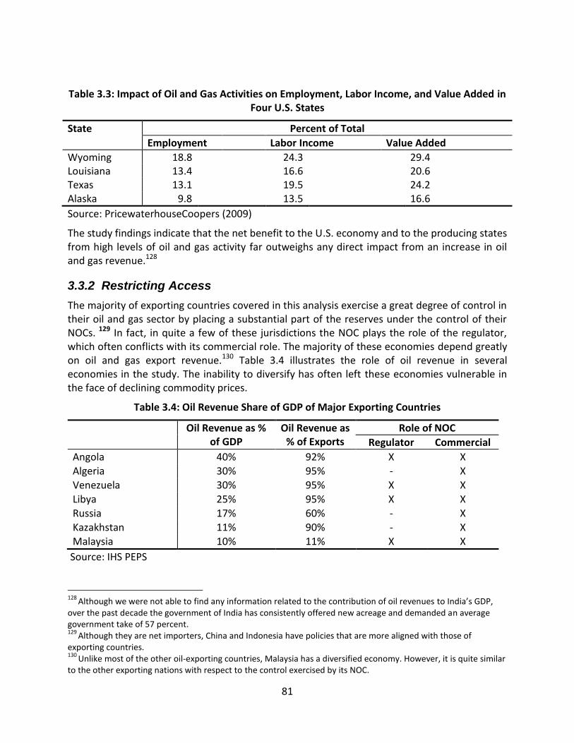
81

Table 3.3: Impact of Oil and Gas Activities on Employment, Labor Income, and Value Added in Four U.S. States

State Percent of Total

Employment Labor Income Value Added

Wyoming 18.8 24.3 29.4 Louisiana 13.4 16.6 20.6 Texas 13.1 19.5 24.2 Alaska 9.8 13.5 16.6

Source: PricewaterhouseCoopers (2009)

The study findings indicate that the net benefit to the U.S. economy and to the producing states from high levels of oil and gas activity far outweighs any direct impact from an increase in oil and gas revenue.128

3.3.2 Restricting Access

The majority of exporting countries covered in this analysis exercise a great degree of control in their oil and gas sector by placing a substantial part of the reserves under the control of their NOCs. 129 In fact, in quite a few of these jurisdictions the NOC plays the role of the regulator, which often conflicts with its commercial role. The majority of these economies depend greatly on oil and gas export revenue.130 Table 3.4 illustrates the role of oil revenue in several economies in the study. The inability to diversify has often left these economies vulnerable in the face of declining commodity prices.

Table 3.4: Oil Revenue Share of GDP of Major Exporting Countries

Oil Revenue as % of GDP

Oil Revenue as % of Exports

Role of NOC

Regulator Commercial

Angola 40% 92% X X Algeria 30% 95% - X Venezuela 30% 95% X X

Libya 25% 95% X X Russia 17% 60% - X Kazakhstan 11% 90% - X Malaysia 10% 11% X X

Source: IHS PEPS

128

Although we were not able to find any information related to the contribution of oil revenues to India’s GDP, over the past decade the government of India has consistently offered new acreage and demanded an average government take of 57 percent. 129

Although they are net importers, China and Indonesia have policies that are more aligned with those of exporting countries. 130

Unlike most of the other oil-exporting countries, Malaysia has a diversified economy. However, it is quite similar to the other exporting nations with respect to the control exercised by its NOC.

82

A common characteristic among these oil exporting jurisdictions is that they do not offer acreage on a regular basis, as is done in Canada, Australia, parts of the United States, and the United Kingdom. These countries usually demand a very high government take, and, except for Malaysia, they have very unstable fiscal systems.

They often experience periods of high and low investments, which are also reflected in production fluctuations. The periods of low investment are sometimes a result of government decisions to withdraw acreage when commodity prices drop.

3.3.3 Mixed Approaches

Other resource holders covered in this study, in spite of the different socioeconomic drivers, appear to share similar goals with both camps—net exporters and net importers. Over the past decade Brazil’s approach to attracting investment in the oil sector has been quite similar to that of the United States. In fact, Brazil’s bidding rounds mimicked the ones in the GOM with respect to block sizes and signature bonuses.131 Brazil’s objectives were somewhat different, however. In addition to increasing investment in the country, the government focused on increasing local content.132 Building local capabilities and participation was just as important to the government as attracting investment. A combination of good geology, intensified drilling activity, and reasonable levels of government take (similar to that in the GOM) helped Brazil shift its position from a net importer of crude oil to a net exporter in 2009, according to data from the EIA.

As the perception about Brazil’s prospectivity skyrocketed in 2008–09, the government decided to exercise a greater degree of control over oil and gas production by introducing mandatory participation by its NOC and also introducing production sharing as one of the models to be adopted for future acreage allocation. Given the experience of Petrobras as Brazil’s operator offshore and the fact that international oil companies had already partnered with Petrobras in the past, this particular measure does not appear to have had any detrimental effect on E&P activity in this jurisdiction.

Unlike the other exporting countries, Norway is a developed economy. In spite of the diversification of its economy, oil revenue makes up 30 percent of its GDP and 45 percent of its export earnings. It has the largest sovereign fund, $500 billion, saved for future generations. As in most exporting countries, though, the government has had a “go slow” policy.133 At the heart of this policy is the objective of conserving petroleum resources for future generations; this has been implemented through control of the rate of depletion of the resources.134 Although the policy of a controlled depletion rate is still in force, a more recent policy calls for rapid development of mature areas to utilize existing infrastructure prior to the end of its useful life.

131

Since 1998 Brazil has offered acreage on a regular basis (annually)—with a few exceptions in recent years, when the government was contemplating a policy change. In 2003 Brazil reduced the size of an offshore block from an average of 4,555 square km per block in 2009 to 262 square km. See Jacqueline Mariano and Emilio La Rovere, “Oil and Gas Exploration and Production Activities in Brazil: The Consideration of Environmental Issues in the Bidding Rounds Promoted by the National Petroleum Agency,” Energy Policy 35 (2007), 2899–2911. 132

According to data from Brazil’s National Oil Regulatory Agency, the average local content commitment during exploration phase increased from 25 percent in 1999 to almost 86 percent in 2004. 133

Storting, An Industry for the Future—Norway’s Petroleum Activities. White Paper 28 (2010). 134

Hunter.

83

Norway has been able to sustain reasonable levels of activity on its share of the North Sea by providing a stable and attractive investment environment that yields a reasonable return on investments. Although it is often referred to as an example of high government take, the Norway fiscal system is still very attractive because it is based purely on taxation of profits rather than gross revenue.

3.3.4 New Markets

Germany, Poland, and Queensland (Australia) represent relatively new markets for international oil companies.135 The technological advances that made the unconventional gas revolution possible in the United States have opened these markets to international oil companies. The perception of prospectivity and their relatively low levels of government take have drawn investors to these jurisdictions just as activity levels in some of the major petroleum jurisdictions have dropped down significantly. It remains to be seen whether the companies will be able to overcome environmental challenges and other aboveground risks associated with the development of shale gas in a densely populated Europe.

3.3.5 Evolving Energy Policies and the Environment

In spite of the generalizations made in this study and the attempt to group countries into categories, energy policies are much more complex and evolve with the evolution of the socioeconomic drivers behind them.136 Often concerns about the environment and climate change have a significant impact on energy policy related to fossil fuels in general and the oil and gas sector in particular. The way governments approach environmental concerns varies by country and sometimes by location within the same jurisdiction. Even when these concerns are not directly reflected in fiscal policy through carbon taxes, the cost of compliance with environmental regulation is often reflected in the cost of doing business in a particular jurisdiction.

Environmental legislation in North America is much more prescriptive than in other parts of the world, where governments adopt a goal-setting approach. Both approaches are designed to reach the same goal: protection of the environment. The prescriptive approach, however, places a greater administrative burden on companies in terms of permitting and reporting requirements. This ultimately affects the cost of doing business in a particular jurisdiction and is factored into the considerations that go into investment decisions and projecting future cash flows.

135

Germany and Poland are not new to the oil and gas industry per se. Their conventional oil and gas potential was not significant enough to attract international oil and gas companies. The market was dominated by local operators. 136

Tordo, Johnston, and Johnston, Countries’ Experience with the Allocation of Petroleum Exploration and Production Rights, xii, “Country-specific objectives and constraints tend to change over time, as do exogenous factors.”

84

4. RANKING BY GOVERNMENT TAKE AND OTHER INDICATORS

4.1 Approach

Our approach to ranking of fiscal systems in respect to fiscal terms relies on an index of four variables: government take, profit-to-investment ratio (PI), internal rate of return (IRR) and progressivity/regressivity. The combination of the chosen variables sheds light on various aspects of the fiscal system. This approach provides for a comparison of fiscal systems from both the government and investor perspectives. An analysis of measures of profitability is important to gauge whether prospects in a particular jurisdiction are competitive in the international market as well as whether they are economic under the current cost and market prices. Reliance on measures of profitability is essential to determine whether the current and suggested royalty frameworks strike the proper balance between the attractiveness of the federal leases for investment and appropriate returns to the federal government for the oil and gas resources.

Government Take. The definition and limitations of this indicator are discussed at length in the previous chapter.

Profit-to-Investment Ratio. The PI indicator measures profitability by comparing the proposed project’s cash flows to the capital investments required and is one of the most commonly used tools for evaluating investments. It allows companies to identify the relationship of investment to payoff of a proposed project. It is calculated as the ratio between the net present value (NPV) of the sum of project cash flow and total capital invested to the NPV of the total capital invested. The PI indicator measures the profitability per dollar invested: a PI of 1.20 means that for every dollar invested in the project the total value created is $1.20, or a net profit of $0.20 per dollar invested. The PI is a decision criterion for ranking investments when capital is constrained.

The discount factor used to calculate PI will vary with each investor. Sometimes different projects are assigned different discount factors depending on the risk. In the decision-making process companies do not proceed with projects that yield a PI of less than one. That would indicate that the NPV of capital invested exceeds the NPV of cash inflows. For this study we have used a 10 percent discount rate.137 The choice of the discount rate depends on a number of factors, including the company’s cost of capital and the desired IRR.

Internal Rate of Return. Investor IRR expresses the nominal discount rate that would generate an NPV of zero when applied to the investor's net cash flow after all levies and taxes (and after direct state participation, where relevant). Projects with an IRR lower than the target rate, or threshold rate, are not usually pursued. Although threshold rates are unique to each company,

137

The US Securities and Exchange Commission requires 10 percent in filings for public companies. See Rhett G. Campbell, “Valuing Oil and Gas Assets in the Courtroom,” presented at the American Institute of Business Law in conjunction with the Oklahoma Bar Review and the Conference on Consumer Finance Law, February 7-8, 2002.

85

a 15 percent rate of return is quite common.138 The IRR method does have one significant advantage: managers tend to better understand the concept of returns stated in percentages and find it easy to compare them to other opportunities. However, the use of the IRR indicator can lead to the belief that a smaller project with a shorter life and earlier cash inflows is preferable to a larger project that will eventually generate more cash.

Despite its widespread use, the IRR indicator has its limitations. It assumes reinvestment of interim cash flows in projects with equal rates of return. When a project’s interim cash flows are reinvested at a rate lower than the calculated IRR, the IRR approach overstates the annual equivalent rate of return. Quite often there may be no other project in the interim that can earn the same rate of return as the original project. Thus, when the IRR appears to be very high (higher than the true reinvestment rate), it is not a reliable measure because it overstates significantly the annual equivalent return from the project.139

Progressivity/Regressivity. Unlike the PI and IRR indicators that measure profitability, the fourth measure we use for this particular index looks at the relationship between the government take and project profitability. This relationship is significant, as it can influence investment decisions as well as investor behavior. When the relationship is inverse, i.e., the government take declines as profitability increases, or vice versa, the fiscal system is considered regressive. Such fiscal systems affect investment decisions and hinder the development of marginal fields. When the relationship between government take and profitability is direct, i.e., government take increases as profitability goes up, or vice versa, the fiscal system is considered progressive. Such fiscal systems usually allow the government to capture the upside when project profitability increases as a result of high prices, growing reserves, lower costs, and other factors.

Each fiscal system in our ranking is assigned a score of zero to five. A score of five represents the government perspective—high government take, low PI, low IRR, and a highly progressive or regressive fiscal system. On the other end of the spectrum, a score of zero is favorable to investors and represents a low government take, high IRR, high PI, and a neutral fiscal system. All four variables are assigned an equal weight of 25 percent to combine into a single index score to measure the relative attractiveness of fiscal terms from both the government and investor perspectives. This chapter analyzes the results for each variable, both individually and combined.

4.2 Government Take and Profitability Indicators

4.2.1 Offshore Fiscal Systems

The analysis of 153 fields modeled for this study shows that on average the government take from offshore projects was higher than the average take related to onshore projects, 74 and 70 percent, respectively. Although this may be partially attributed to the features of the specific fiscal systems included in the study, the main reason for the high take is the costs associated

138

Tordo, Fiscal Systems for Hydrocarbons, 28. 139 Another issue with the IRR indicator is that a single project can have more than one rate of return when cash flow switches from positive to negative and turns positive again.

86

with offshore development. Even in the U.S. GOM there is a significant difference in government take between the mature areas of the shelf and the more prospective deepwater and ultradeepwater acreage, even though the fiscal systems are identical.140 Although costs are generally lower in the shelf compared to the deepwater, the relatively small size of discoveries and the depth of formations result in a higher per-unit cost of finding and development in the shelf.141

The average government take under all three price and cost scenarios adopted for this study is 79 percent for the GOM shelf area. The average take under the low price and cost scenario is 96 percent. The low gas price of $4 per Mcf of gas adopted for this study is actually closer to the currently prevailing natural gas prices in the United States. Under our base price and cost scenario of $6 per Mcf of gas and $75 per barrel of oil, the government take averages around 74 percent. The take drops to 66 percent under the high price assumption of $8 per Mcf of gas and $105 per barrel of oil.

Although this analysis of government take shows that on average the take in the GOM shelf is higher than the worldwide average of 72 percent and the offshore average of 74 percent, by itself it fails to reveal the rather marginal nature of profits. The profitability indicators are not simply below average; they are undesirable. Even with the field selection skewed toward the limited number of fields that rank in the ninetieth percentile for the GOM shelf region, this jurisdiction compares poorly with other offshore systems as well as globally. The average PI at a discount factor of 10 percent is 0.72, which means that for every dollar invested, the total value created is $0.72. The IRR indicator also shows poor rates of return, averaging 4 percent. Even under our high price assumption of $8 per Mcf of gas and $105 per barrel of oil, the PI ratio and IRR remain rather low, at 0.89 and 8 percent, respectively. Figures 4.1.a and 4.1.b show cash flow components of the natural gas and oil fields in the GOM shelf modeled for this study. Government take and other indicators for each project for all jurisdictions are shown in Appendix III.

The combined government take for the seven gas fields on the shelf is 100 percent. While government Income represents 21 percent of the combined cash flow from the seven gas fields selected for this study, investor income is minus seven percent of the combined cash flow. When the results of the three oil fields are combined, the government take as a percentage of total cash flow is 25 percent, compared with company income of 8 percent. The combined government take for all five projects is greater than 75 percent.

140

The only difference lies in area rentals, which are not significant enough to cause the difference in government take. 141

The discoveries on the shelf were mostly found in deep and ultradeep gas formations, which are very expensive to develop.

87

Figure 4.1.a: Undiscounted Cash Flow Components of Seven Gulf of Mexico Shelf Natural Gas Fields

-$1,000

$0

$1,000

$2,000

$3,000

$4,000

$5,000

$6,000

$7,000

Gas Field 1 Gas Field 2 Gas Field 3 Gas Field 4 Gas Field 5 Gas Field 6 Gas Field 7

Mill

ion

Do

llars

U.S. GOM Shelf Gas Fields

Company Income

Income Taxes

Bonus and Rental

Royalty

Operating Expenses

Capital Expenditure

Company Income -7% of Cash FlowGovernment Income 21% of Cash Flow>100% Government TakeSix fields rank >90% for the region

Source: IHS CERA

59%

>100% >100% >100%

>100%

61%

>100%

Figure 4.1.b: Undiscounted Cash Flow Components of Three Gulf of Mexico Shelf Oil Fields

-$500

$0

$500

$1,000

$1,500

$2,000

$2,500

$3,000

$3,500

Oil Field 1 Oil Field 2 Oil Field 3

Mill

ion D

olla

rs

U.S. GOM Shelf Oil Fields

Company Income

Income Taxes

Bonus and Rental

Royalty

Operating Expenses

Capital Expenditure


Source: IHS CERA

63%

87%

>100%

88

Unlike the GOM shelf area, which has reached maturity, the deepwater and ultradeepwater areas of the GOM are much more prospective. This is evidenced by the significantly larger reserves discovered during the past ten years. The recoverable reserves for the GOM shelf oil fields modeled for this study range between 4 and 40 million barrels, compared with the recoverable reserves for the deepwater and ultradeepwater fields, which range between 30 and 600 million barrels of oil.

The government take for deepwater acreage averages 73 percent under our low price and cost scenario, 61 percent under the base price and cost scenario, and 57 percent under the high price and cost scenario. The deepwater oil fields modeled for this study yield acceptable IRRs ranging between 10 and 15 percent under the base price and cost scenario. Natural gas projects, however, are highly unprofitable under all three price and cost scenarios. Figures 4.2.a and 4.2.b show the cash flow components of the deepwater oil and gas fields modeled for this study. When the results of the five deepwater gas fields are combined, the government take as a percentage of total cash flow is 21 percent, compared with company income of minus 69 percent. The combined government take for all five projects is greater than 100 percent. When the results of the five deepwater oil fields are combined, the government take as a percentage of total cash flow is 34 percent, compared with company income of 28 percent. The combined government take is 55 percent.

Figure 4.2.a: Undiscounted Cash Flow Components of Five Gulf of Mexico Deepwater Gas Fields

-$1,500

-$1,000

-$500

$0

$500

$1,000

$1,500

$2,000

$2,500

$3,000

$3,500

Gas Field 1 Gas Field 2 Gas Field 3 Gas Field 4 Gas Field 5

Mil

lio

n D

oll

ars

U.S. GOM Deepwater Gas Fileds

Company IncomeIncome TaxesBonus and RentalRoyaltyOperating ExpensesCapital Expenditure

Company Income - 69% of Cash FlowGovernment Income 21% of Cash Flow>100% Government Take

Source: IHS CERA

>100%

>100%86%

>100% >100%

89

Figure 4.2.b: Undiscounted Cash Flow Components of Five Gulf of Mexico Deepwater Oil Fields

$0

$5,000

$10,000

$15,000

$20,000

$25,000

$30,000

$35,000

$40,000

$45,000

$50,000

Oil Field 1 Oil Field 2 Oil Field 3 Oil Field 4 Oil Field 5

Mill

ion

Do

llars

U.S. GOM Deepwater Oil Fields

Company Income

Income Taxes

Bonus and Rental

Royalty

Operating Expenses

Capital Expenditure

Company Income 28% of Cash FlowGovenrment Income 34% of Cash Flow55% Government Take

Source: IHS CERA

56%

54%

54%

57%

58%

Figures 4.3.a–c compare offshore fiscal systems on the basis of government take and profitability indicators. To some extent, these offshore jurisdictions are comparable in terms of finding and development costs.142 The distinguishing feature in most cases is the fiscal system. The front-end loaded payments in the GOM fiscal systems increase the marginal cost of finding and development, rendering these systems less attractive than the majority of the offshore fiscal systems covered in this study. The levy of royalties at rates that are unusually high for offshore exploration and production contributes to the rather low profitability indicators in the GOM.

142

Cost on average ranged between $20 and $30 per barrel among most jurisdictions.

90

Figure 4.3.a: Percentage of Average Government Take—Offshore Fiscal Systems

62%

63%

64%

71%

72%

78%

78%

79%

79%

80%

82%

93%

0% 10% 20% 30% 40% 50% 60% 70% 80% 90% 100%


India offshore

U.S. GOM deepwater

Australia offshore

Brazil offshore

Angola offshore

Kazakhstan offshore

U.S. GOM shelf

Norway offshore

China offshore


Malaysia offshore


Figure 4.3.b: Average PI—Offshore Fiscal Systems

1.62

1.57

1.46

1.32

1.19

1.17

1.13

1.07

1.04

1.04

0.93

0.72

- 0.20 0.40 0.60 0.80 1.00 1.20 1.40 1.60 1.80

Brazil offshore

Australia offshore

China offshore

Angola offshore

India offshore

Kazakhstan offshore



U.S. GOM deepwater

Norway offshore

Malaysia offshore

U.S. GOM shelf

Average PISource: IHS CERA

91

Figure 4.3.c: Average IRR—Offshore Fiscal Systems

20%

16%

14%

14%

13%

12%

12%

12%

11%

10%

7%

4%

0% 5% 10% 15% 20% 25%

Australia offshore

Angola offshore

Brazil offshore

India offshore

Kazakhstan offshore

China offshore


Norway offshore


U.S. GOM deepwater

Malaysia offshore

U.S. GOM shelf

Average IRRSource: IHS CERA

4.2.2 North American Fiscal Systems

A comparison of North American onshore fiscal systems against other onshore fiscal systems covered in this study shows that the regional average government take is about the same: 69 percent in North America and 70 percent worldwide. However, there is a wider gap among profitability indicators, particularly with respect to PI. The average PI for North American projects is 1.06, compared with the worldwide average of 1.22 onshore and 1.16 offshore. In particular, the fiscal systems of the United States strongly favor the resource holder.

Of the four U.S. onshore jurisdictions included in this study, Wyoming federal lands levy the lowest average government take: 66 percent compared with 76 percent in Alaska and Texas and 85 percent in Louisiana. Although averages are useful when comparing multiple projects per jurisdiction, they may not be very reliable when one or two fields skew the average significantly. An examination of the results of the conventional fields in Wyoming reveals that four out of five conventional gas projects were not profitable and resulted in a greater than 100 percent government take. Figure 4.4 shows the cash flow components of the five conventional gas fields in Wyoming. When the results of the five fields are combined, the government take as a percentage of total cash flow is 31 percent, compared with company income of zero percent. The combined government take for all five projects is greater than 100 percent.

92

Figure 4.4: Undiscounted Cash Flow Components of Five Wyoming Conventional Gas Fields

-$50

$0

$50

$100

$150

$200

$250

Conventional Gas Field 1





Mill

ion

Do

llars

Wyoming Conventional Gas Fields

Company Income

Income Taxes

Production Taxes

Royalty

Bonus and Rental

Operating Expenses

Capital Expenditure

Company Income 0% of Cash FlowGovernment Income 31% of Cash Flow>100% Government Take

Source: IHS CERA

55%

> 100% > 100%

> 100% > 100%

The poor economic performance of the fields modeled for this study is largely due to the rather low well productivity and the small size of recoverable reserves associated with new-field wildcat discoveries made in the past decade. The combined reserves for the five conventional gas fields selected for this study were 7.61 MMboe, compared with the total of 46.13 MMboe for three natural gas fields in Texas and 60.71 for the conventional gas fields in Louisiana. The limited number of new-field wildcat discoveries—20 total over the past decade—and the rather small size of the discoveries have affected investor perception of prospectivity in the jurisdiction. This perception is reflected in bonus bids payable per acre on Wyoming federal lands. In general, companies have been willing to pay more for acquisition of rights on state land in Louisiana and Texas than in Wyoming and Alaska. The average bid per acre over the past five years in Wyoming has been the lowest among North American jurisdictions, after Alaska. Since 2006 the average bonus bid in Wyoming has been $76 per acre, compared with $1,115 per acre in Louisiana, $841 per acre in British Columbia, $439 per acre in Texas, $191 per acre in Alberta, and $21 per acre in Alaska.

Coalbed gas projects in Wyoming perform marginally better, largely because of a processing cost allowance for royalty purposes. The cost of compressing coalbed gas can be significant enough to result in an effective royalty rate of 8 percent. Figure 4.5 shows the undiscounted cash flow components of the Wyoming coalbed gas projects. When the results of the five coalbed gas fields are combined, the government take as a percentage of total cash flow is 28 percent, compared with company income of fifteen percent. The combined government take for all five projects is 66 percent.

93

Figure 4.5: Undiscounted Cash Flow Components of Five Wyoming Coalbed Gas Fields

50%

73%

59%

58%59%

$0

$500

$1,000

$1,500

$2,000

$2,500

$3,000

$3,500

$4,000

$4,500

$5,000

Coalbed Gas Field 1

Coalbed Gas Field 2

Coalbed Gas Field 3

Coalbed Gas Field 4

Coalbed Gas Field 5

Mill

ion

Do

llars


Government Take

Company Income

Income Taxes

Production Taxes

Royalty

Bonus and Rental

Operating Expenses

Capital Expenditure


Source: IHS CERA

With the exception of the Alberta oil sands fiscal system, the Canadian fiscal systems are more attractive for investors than the U.S. fiscal systems included in this study, based on government take as well as profitability indicators. After a temporary setback resulting from the revision of royalty rates in 2007, the province of Alberta has been able to reverse course and attract investment in its mature conventional oil and gas sector. A recent competitiveness review conducted by the government of Alberta acknowledged that the province had lost competitive ground to the neighboring provinces of British Columbia and Saskatchewan and to the United States. British Columbia has seen an unprecedented level of activity, particularly after the introduction of the net revenue royalty to encourage investment in shale gas resources. These two provinces with significant potential in shale gas and coalbed gas have positioned themselves as major competitors with the United States for investment in their natural gas sector.

As a gas-prone jurisdiction, Wyoming is competing for investments not just with its neighbors in the United States. The determination of the Canadian provinces to maintain their position as a major supplier of natural gas to the United States could lead to a race to soften, rather than increase, the fiscal burden. Since 2009 the provinces of Alberta and British Columbia have competed with each other, which resulted in several incentives for the industry.

Given this shift in the competitive landscape since the time the GAO report was written and released, the main question should be whether Wyoming is competitive. Figure 4.6 compares the North American onshore oil and gas fiscal systems placing Wyoming fourth among seven jurisdictions with regard to government take. Although average profitability indicators fall

94

within a reasonable range, the limited number of conventional oil and gas discoveries over the past ten years and the low bonus bids per acre compared with the select peer group raise doubts about the competitive position of the federal lands fiscal system for conventional and coalbed gas in Wyoming.143

4.3 Fiscal System Flexibility

The commodity price fluctuations over the past five years have often raised questions about the suitability of existing fiscal systems. Even within the United States, the GAO has suggested introducing a fiscal system that has built-in flexibility to automatically adjust to changing economic and market conditions. Although that goal is much sought after by many resource holders, to date no one has been able to achieve that kind of flexibility.144 The fact that almost every nation with significant resource potential has introduced changes at least once and, in many cases, two to three times over the past five years suggests that they have not been able to strike the right balance. There is no such thing as a perfect fiscal system; each one has advantages and disadvantages. Attempts to introduce built-in flexibility in the fiscal system quite often have resulted in rigid fiscal systems as market conditions change over time. Introducing price thresholds does not always result in built-in flexibility. In fact, if there is a dramatic shift in commodity prices, one that could not have been anticipated at the time the fiscal system was designed, the fiscal system does not work. Figure 4.7 shows some of the price thresholds adopted in various fiscal instruments by a number of countries over the past decade. Although they were all designed to capture the upside when the commodity prices exceeded the base price (the so-called windfall price), in the current investment environment where costs have gone up significantly, most of the base prices, including those established two to three years ago, can hardly be considered windfall prices in their respective jurisdictions.

For the purpose of this study, the degree of progressivity and regressivity of each fiscal system was examined to determine the risk exposure to the government and the contractor. Theoretically progressive fiscal systems should appeal to governments and investors alike. However, in reality they are very difficult to achieve. Of the 29 fiscal systems analyzed in this study, only 6 are truly progressive ones. In fact, some of the most regressive fiscal systems are ones that already adopt fiscal instruments tied to oil prices or payout, such as Alberta conventional and Alberta oil sands.

143

A range of IRR between 13 and 18 percent was considered reasonable by the Alberta Royalty Review Panel in 2007. See Van Meurs, “Comparative Analysis.” 144

Bryan Land, “Capturing a Fair Share of Fiscal Benefits in the Extractive Industries,” Transnational Corporations Journal 18 no. 1 (2009), 157–174.

95

Figure 4.6: Comparison of North American Onshore Fiscal Systems—Government Take and Profitability Indicators

40%

59%

61%

66%

76%

76%

85%

0% 50% 100%

Canada (British

Columbia)



U.S. Wyoming gas

U.S. Texas onshore

U.S. Alaska onshore

U.S. Louisiana

onshore gas

GOV Take

1.32

1.22

1.17

1.09

1.03

0.95

0.92

- 0.50 1.00 1.50


U.S. Wyoming gas


U.S. Alaska onshore

U.S. Louisiana onshore

gas

U.S. Texas onshore


PI

27%

16%

14%

13%

11%

11%

9%

0% 10% 20% 30%



U.S. Wyoming gas


U.S. Alaska onshore

U.S. Texas onshore


IRR

Source IHS CERA

96

A progressive fiscal system is one in which government take increases as profitability increases and declines as profitability drops. Using fiscal instruments that change with the commodity price but are not responsive to cost changes does not make a fiscal system progressive. In fact, if costs escalate at a higher pace than the commodity price, the system becomes rather regressive. Payments made early on in the project life, when there is no revenue stream, are considered regressive. Fiscal levies that are based on gross revenues rather than net revenues are inherently regressive, regardless of the ability to change as commodity prices change. Signature bonuses, training fees, and rentals are included in this category. State participation through carried interest is another means of taxation. This, too, is considered to be regressive. Royalty and severance taxes under concessionary systems and cost recovery ceiling or government allocation under production sharing schemes are means of securing revenue up front for the government. Although these instruments may not be as regressive as signature bonuses, they are not based on project profits, and therefore they are regressive in nature. Fiscal instruments that tax net revenue are considered progressive. Most fiscal systems use a combination of progressive and regressive elements. Very few governments rely entirely on profit-based levies to generate revenue from upstream oil and gas investments.

Figure 4.7: Rigid Price Thresholds Adopted by Select Countries

$0 $20 $40 $60 $80 $100 $120 $140

Pakistan***

Egypt

Venezuela

Hungary

U.S. Alaska


Algeria

China

Ecuador**

Colombia

Russia

Argentina*

Oil Price

Base Price

Maximum Price

$343

$200

2002

2003

2004

2006

2006

2006

2007

2007

2008

2008

2008

20092001

Year Adopted

Source: IHS CERA *In 2007 Argentina introduced legislation by means of which the government is entitled to all incremental revenue above $42 per barrel. **Ecuador base price is the price of oil prevailing at the time the contract was signed. We have assumed $18 for Round 8 contracts. ***In Pakistan the base price was established in 2001, whereas the maximum threshold was established in 2009.

97

To assess the fiscal system flexibility, our analysis focused on the behavior of each fiscal system as IRRs increased from 5 percent to 25 percent. Based on the relative degree of change in government take, fiscal systems were assigned a score of zero to five, with neutral fiscal systems scoring zero. In a neutral fiscal system, government take remains constant while project profitability goes up or down. Such systems do not distort investment decisions. Although it seems desirable from an economic theory perspective, governments do not always rely on neutral tax to generate revenue. Under a neutral fiscal system, the government takes on a significant revenue risk, the possibility of zero revenue if the project is not profitable. Also the government does not reward itself for the revenue risk it takes, i.e., it does not capture the project upside. From an investor point of view, this is a desirable fiscal system, as it does not present any risk and therefore does not distort investment decisions.

Although progressive fiscal systems are desirable, highly progressive fiscal systems pose a significant threat to investors if they tend to capture all of the upside. If not properly designed, they encourage inefficient resource development and provide no incentive to lower costs. For that reason, highly progressive systems are assigned a high score similar to highly regressive systems. Figure 4.8 shows the degree of change in government take as profitability increases from 5 to 25 percent IRR.

Figure 4.8: Degree of Change in Government Take with 20 Percent Increase in IRR

-30%

-20%

-10%

0%

10%

20%

30%

Nor

way

off

shor

e

Kaz

akh

stan

off

sho

re

Ch

ina

off

sho

re

Liby

a on

shor

e

An

gola

off

sho

re

Can

ada

(Bri

tish

Co

lum

bia

)

Uni

ted

Kin

gdom

Col

ombi

a on

shor

e

Vene

zuel

a he

avy

oil

Po

lan

d o

nsh

ore

Aus

tral

ia o

ffsh

ore

Alg

eria

ons

hore

U.S

. Lou

isia

na o

nsho

re g

as

Aus

tral

ia (Q

ueen

slan

d) c

oalb

ed g

as

Ger

man

y on

shor

e

Ind

on

esi

a c

oa

lbe

d g

as

Mal

aysi

a of

fsho

re

Indo

nesi

a co

nven

tion

al g

as o

ffsh

ore

U.S

. Wyo

min

g ga

s

Ve

ne

zue

la c

on

ven

tio

na

l ga

s

Indi

a of

fsho

re

U.S

. GO

M s

helf

U.S

. Tex

as

U.S

. GO

M d

ee

pw

ate

r

U.S

. Ala

ska

on

sho

re

Can

ada

(Alb

erta

) oil

sand

s

Bra

zil o

ffsh

ore

Rus

sia

onsh

ore

Ca

na

da

(Alb

ert

a) c

on

ven

tio

na

l oil

Gov

ernm

ent T

ake

Cha

nge

Source: IHS CERA

98

The results indicate that all three U.S. federal fiscal systems are highly regressive. That is explained by the front-end loaded payments such as signature bonuses and royalties. The only neutral system is for the U.K. offshore, to the degree that the operator can carry back in full losses from abandonment costs.

Fiscal systems are assigned scores of zero to five depending on their degree of progressivity or regressivity. The fiscal systems with the highest degree of progressivity/regressivity get a score of five. A neutral system such as in the United Kingdom is assigned a score of zero. Depending on the degree of progressivity or regressivity, scores are normalized to fall within these two ranges. When ranking fiscal systems from a progressivity or regressivity perspective, the deepwater GOM ranks in the top 20 percent of the fiscal systems analyzed and the GOM shelf and Wyoming fall in the top 30–35 percent range. Figure 4.9 shows the progressivity/regressivity score for each fiscal system.

Figure 4.9: Progressivity/Regressivity Index

0.00

0.67

0.83

1.33

1.33

1.50

1.50

1.67

1.83

2.00

2.00

2.17

2.17

2.67

2.67

2.67

2.83

3.00

3.00

3.17

3.67

3.67

5.00

0.16

0.17

0.52

1.21

1.33

4.50

0.00 1.00 2.00 3.00 4.00 5.00 6.00

United Kingdom offshoreCanada (British Columbia)

Angola offshoreLibya onshore

Colombia onshoreVenezuela heavy oil

China offshoreKazakhstan offshore

Australia offshorePoland onshoreAlgeria onshore

U.S. Louisiana onshoreAustralia (Queensland) coalbed gas

Germany onshoreIndonesia coalbed gas

Malaysia offshoreIndonesia conventional gas offshore

Venezuela conventional gasIndia offshore

U.S. GOM shelfU.S. Wyoming gas

U.S. Texas onshoreU.S. Alaska onshore

U.S. GOM deepwaterCanada (Alberta) oil sands

Brazil offshoreRussia onshore

Norway offshoreCanada (Alberta) conventional oil

Progressivity/Regressivity Index Score

Progressive Regressive

Source: IHS CERA

Highly Regressive/Progressive

4.4 Fiscal Terms Index

In a ranking of offshore fiscal systems based on equal weighting of all four variables, the GOM shelf fiscal system is at the top of the list and the GOM deepwater fiscal system ranks fifth. Reliance on bonus bids and high royalty rates for revenue collection has resulted in the balance weighing in favor of the government. Figure 4.10 shows the ranking of fiscal terms for offshore

99

systems. A combination of low IRR and high government take and a highly regressive fiscal system is likely to result in loss of competitive edge for the GOM shelf fiscal system. Although the deepwater fiscal system does not rank as high as the fiscal system applicable on the shelf, there is potential for the deepwater also to lose competitive ground. The fiscal system has been shown to be vulnerable when commodity prices drop. This vulnerability was manifested in 2009, when there was a significant drop in acreage leased as well as bonus revenue from both areas of the Gulf when commodity prices were low.

Figure 4.10: Fiscal Terms Index—Offshore

0.00 0.50 1.00 1.50 2.00 2.50 3.00 3.50 4.00 4.50

Australia offshore

Angola offshore


China offshore

Brazil offshore

India offshore

Kazakhstan offshore

U.S. GOM deepwater


Malaysia offshore

Norway offshore

U.S. GOM shelf

Fiscal Index Score


Source: IHS CERA

When all four variables are combined into a single index for North America, as in Figure 4.11, Wyoming gas fiscal system ranks fifth among the seven onshore North American jurisdictions. Wyoming, however, faces strong competition from the Canadian jurisdictions of British Columbia and Alberta as well as from the United States jurisdictions with shale gas potential. As traditional sources of gas supply are displaced by the lower-cost shale gas resources, Wyoming could become less competitive. The trend of leasing and the average bonus bid per acre payable on federal lands in Wyoming is significantly lower than the amounts payable in the other jurisdictions, except Alaska.145 The high-cost conventional gas resources that were developed prior to 2008, when commodity prices were high, are no longer competitive under the prevailing market prices. Four out of five conventional gas fields modeled for Wyoming resulted in negative IRR. Figure 4.11 ranks North American onshore jurisdictions based on the

145

There has been a notable increase in bonus bids per acre in 2011 in Wyoming on a number of parcels sold. This is associated with the potential for shale oil development in Niobrara, south of Wyoming. Although this has led to an increase of the average bonus bid per acre from $168 in 2010 to $474 in 2011 (as of October 2011), Wyoming continues to rank below Texas, British Columbia and Louisiana in bonus bids per acre received in 2011.

100

fiscal terms index developed for this study.

Figure 4.11: Fiscal Terms Index—Onshore North America

0.00 0.50 1.00 1.50 2.00 2.50 3.00 3.50



U.S. Wyoming gas


U.S. Alaska onshore


U.S. Texas onshore

Fiscal Index Score


Source: IHS CERA

On a global scale, whereas the U.S. offshore fiscal systems rank on top of each profitability indicator—meaning offering a low IRR and PI—Wyoming ranks in the middle. Since Wyoming does not really compete on a global scale in the same sense that most jurisdictions covered in this study do, the global ranking may not be as meaningful for Wyoming as it is for the offshore federal fiscal systems. Figure 4.12 shows the profitability indicators and government take for all 29 fiscal systems. A ranking of fiscal terms based on all four variables as shown in Figure 4.13 puts all three federal jurisdictions in the top half of the index, which indicates high government take, low IRR, low PI, and highly regressive fiscal terms. The GOM shelf appears to be least favorable to investors among these three jurisdictions, ranking in the top 10 percent, with Wyoming and the GOM deepwater ranking in the top 35–50 percent range.

101

Figure 4.12: Comparison of Federal Fiscal Systems—Government Take and Profitability Indicators

28%

40%

40%

59%

61%

61%

62%

63%

64%

66%

71%

72%

73%

76%

76%

78%

78%

79%

79%

79%

80%

82%

82%

84%

85%

86%

91%

93%

95%

0% 50% 100%

Poland onshore




Germany onshore



India offshore

U.S. GOM deepwater

U.S. Wyoming gas

Australia offshore

Brazil offshore

Russia onshore

U.S. Texas onshore

U.S. Alaska onshore

Angola offshore

Kazakhstan offshore

U.S. GOM shelf


Norway offshore

China offshore


Colombia onshore



Algeria onshore

Libya onshore

Malaysia offshore

Venezuela heavy oil

GOV Take

1.83

1.62

1.57

1.50

1.46

1.43

1.41

1.35

1.32

1.32

1.26

1.22

1.20

1.19

1.17

1.17

1.13

1.09

1.07

1.04

1.04

1.03

0.98

0.95

0.93

0.92

0.80

0.72

0.52

- 0.50 1.00 1.50 2.00

Algeria onshore

Brazil offshore

Australia offshore

Poland onshore

China offshore

Libya onshore



Angola offshore


Russia onshore

U.S. Wyoming gas

Colombia onshore

India offshore

Kazakhstan offshore



U.S. Alaska onshore


U.S. GOM deepwater

Norway offshore



U.S. Texas onshore

Malaysia offshore


Germany onshore

U.S. GOM shelf

Venezuela heavy oil

PI

27%

25%

23%

20%

16%

17%

16%

16%

16%

15%

14%

14%

14%

14%

13%

13%

12%

12%

12%

11%

11%

11%

10%

9%

9%

7%

6%

4%

4%

0% 5% 10% 15% 20% 25% 30%


Algeria onshore


Australia offshore


Libya onshore

Angola offshore

Colombia onshore

Poland onshore


U.S. Wyoming gas

Brazil offshore

Russia onshore

India offshore


Kazakhstan offshore

China offshore


Norway offshore

U.S. Alaska onshore


U.S. Texas onshore

U.S. GOM deepwater



Malaysia offshore

Germany onshore

U.S. GOM shelf

Venezuela heavy oil

IRR

Source: IHS CERA

102

Figure 4.13: Fiscal Terms Index

0.00 1.00 2.00 3.00 4.00 5.00

Poland onshoreAlgeria onshore

Canada (British Columbia)Australia (Queensland) coalbed gas

Australia offshoreAngola offshore

Indonesia coalbed gasUnited Kingdom offshore

U.S. Louisiana onshore gasLibya onshore

Colombia onshoreChina offshoreBrazil offshore

U.S. Wyoming gasIndia offshore

Kazakhstan offshoreCanada (Alberta) conventional oil

Russia onshoreU.S. GOM deepwater

Indonesia conventional gas offshoreGermany onshore

U.S. Alaska onshoreCanada (Alberta) oil sands

U.S. Texas onshoreVenezuela conventional gas

Malaysia offshoreNorway offshore

U.S. GOM shelfVenezuela heavy oil

Fiscal Index Score

Gov Take

PI

IRR


Source: IHS CERA

103

5. REVENUE RISK DISTRIBUTION

5.1 Sources of Risk

The high level of uncertainty associated with oil and gas exploration and development raises serious questions as to who should undertake the risk and to what extent the government should, as resource holder, share in the project risk. The sources of risk are varied, and they can occur at all stages of an upstream oil and gas venture. Some of the main risks associated with oil and gas exploration and development are the following:

Geological and geophysical risks. These relate to the probability of finding substantial technically and economically recoverable deposits. Such risks accompany all phases of an upstream venture. It is only when the deposit is fully exhausted that operators know precisely the size of the reserve.146

Price. Price volatility is one of the major risks that upstream oil and gas investments face throughout the project life. While high commodity prices may lead to significant upside, depressed prices can have a devastating impact on project economics and may at times cause the premature cessation of upstream activities.

Cost. As commodity prices rise, the associated demand for goods and services usually drives the cost up. This has a definite impact on project economics and, ultimately, on the before-tax profit to be shared between the government and the investor.

Who should undertake the risk and in what measure is a policy decision.147 Whereas companies hedge against risk by investing in a diverse global portfolio of projects, governments hedge against risk by transferring part of it to the private investors.148 There is a fundamental conflict between the government and the oil companies over the division of risk and reward from an upstream oil and gas investment.149 Each party wants to maximize rewards and shift as much risk as possible to the other party. The choice and the design of the petroleum fiscal system reflect the trade-off between each party’s interests.

Depending on the system adopted for awarding acreage, the fiscal instruments incorporated in the design, and the involvement of the national oil company, the degree of risk sharing by host governments varies significantly. Fiscal systems that front-end load the government revenue shift all the revenue risk to the investor. Signature bonuses, cost recovery ceilings, and ad valorem levies, such as royalties or severance taxes, are some of the fiscal instruments that allow the government to generate revenue up front. On the other hand, governments that use profit-based fiscal instruments usually share the upside; however, they also share the risk of

146

Andrews-Speed, 13–21. 147

Tordo, Johnston, and Johnston, Countries’ Experience with the Allocation of Petroleum Exploration and Production Rights, viii. 148

Tordo, Johnston, and Johnston. 149

Sunley, Baunsgaard, Simard, Revenue from the Oil and Gas Sector, 1.

104

not generating any revenue at all should the project be unprofitable.150 Table 5.1 displays the degree of risk exposure associated with each fiscal instrument.

Table 5.1 Revenue Risk—Fiscal Instruments

Fiscal Instrument Risk to Government

Bonus payments Low

Ad valorem payments (royalty, severance tax, export duty) Low

Cost recovery ceiling Low

Corporate income tax Medium

Resource rent tax High

Profit sharing Medium

Equity participation High

Source: IHS CERA

When governments take on equity interest in the project, their risk exposure is even higher. In addition to sharing the revenue risk, they are sharing the cost with the investor. This higher risk for the government, resulting from its equity participation, does not always mean a lower risk for the investor. The risks associated with the government’s ability to meet the cash-call requirements during the development phase render this kind of arrangement less attractive for investors. Also the type of state participation is important. When participating on a carried-interest basis, which is often the case, the government risk is minimized by allocating the risk of unsuccessful exploration to the investor. Table 5.2 identifies fiscal components found in each jurisdiction with respect to timing of revenue to the government as well as sharing of cost and revenue risk.

150

Sunley, Baunsgaard, Simard, Revenue from the Oil and Gas Sector, 2.

105

Table 5.2: Fiscal System Components

Fiscal System Timing of Revenue Sharing of Revenue and Cost Risk

Bonus Ad Valorem

Cost Recovery Ceiling

Income Tax

Revenue Sharing

State Participation

Income Tax

Resource Rent Tax

Net Revenue-based Royalties

Profit Sharing

Algeria onshore √ √ - √ √ √ √ √ - -

Angola offshore √ - √ √ √ √ √ - - √

Australia (Queensland) coalbed gas - √ - √ - - √ - - -

Australia offshore - - - √ √ - √ √ - -

Brazil offshore √ √ - √ √ √ √ √ - √

Canada (Alberta) conventional oil √ √ - √ - - √ - - -

Canada (Alberta) oil sands √ √ - √ - - √ - √ -

Canada (British Columbia) √ √ - √ - - √ - √ -

China offshore √ √ √ √ √ √ √ √ - √

Colombia onshore - √ - √ √ - √ √ - -

Germany onshore - √ - √ - - √ - - -

India offshore - √ - √ √ - √ - - √

Indonesia coalbed gas √ - √ √ √ - √ - - √


√ - √ √ √ - √ - - √

Kazakhstan offshore √ √ - √ √ √ √ √ √ -

Libya onshore √ - √ √ √ √ √ - - √

Malaysia offshore - √ √ √ √ √ √ √ - √

Norway offshore - - - √ √ - √ √ - -

Poland onshore - √ - √ - - √ - - -

Russia onshore √ √ - √ - √ √ - - -

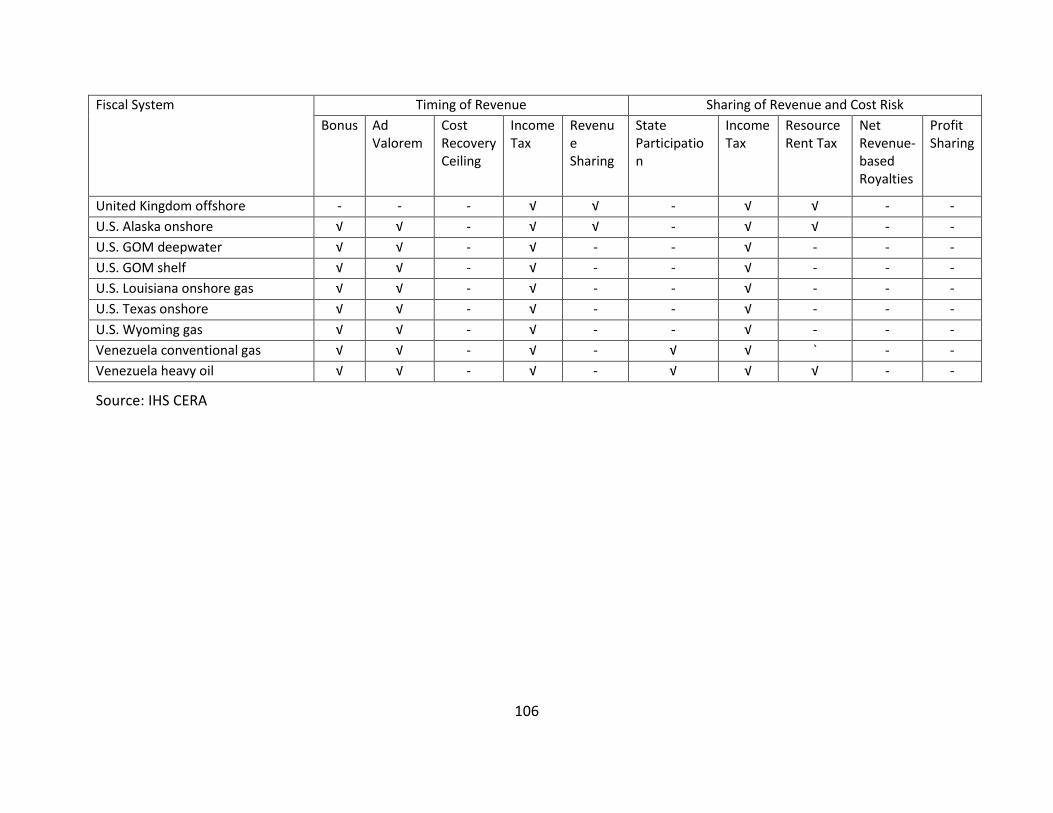
106

Fiscal System Timing of Revenue Sharing of Revenue and Cost Risk

Bonus Ad Valorem


Income Tax

Revenue Sharing

State Participation

Income Tax

Resource Rent Tax

Net Revenue-based Royalties

Profit Sharing

United Kingdom offshore - - - √ √ - √ √ - -

U.S. Alaska onshore √ √ - √ √ - √ √ - -

U.S. GOM deepwater √ √ - √ - - √ - - -

U.S. GOM shelf √ √ - √ - - √ - - -

U.S. Louisiana onshore gas √ √ - √ - - √ - - -

U.S. Texas onshore √ √ - √ - - √ - - -

U.S. Wyoming gas √ √ - √ - - √ - - -

Venezuela conventional gas √ √ - √ - √ √ ` - -

Venezuela heavy oil √ √ - √ - √ √ √ - -

Source: IHS CERA

107

5.2 Risk-Reward Structure of Federal Fiscal Systems

5.2.1 Bonus Bids

The federal oil and gas fiscal systems rely heavily on bonus bids for the allocation of acreage. These upfront payments for the right to explore and produce provide no guarantee that the lessee will be able to discover oil and gas in paying quantities, effectively shifting the risk of exploration onto the oil companies. The amount of bids payable depends largely on

Perceived prospectivity of the jurisdiction. The relative maturity of a geological basin affects the level of competition and the size of the winning bids.151 This explains the relatively lower per acre bid size received in Wyoming and the GOM shelf areas compared with the deepwater GOM. Table 5.3 shows the bonus bids per acre in these jurisdictions since 2001.

Expected future oil and gas prices. Price expectations affect the number of bids as well as the bid size for the same geological basin. That explains the variability over time of the average bid per acre received for rights on federal lands. Thus, in 2007 and 2008, as oil prices were steadily going up, the number of bids in the GOM and the average bid per acre were high, largely because of expectations that prices would persist at those levels or continue to rise. In 2009 the depressed commodity prices combined with the global economic crises contributed to a decline in total acreage sold as well as in the average bid per acre.152

Overall sharing of risks and rewards between government and investor. Depending on the design of the fiscal system and the degree of risk undertaken by the government, investors adjust their expected rate of return when they bid for acreage. Thus, in a system in which government revenue is front-end loaded, the investors are likely to seek a higher rate of return compared with a jurisdiction that allows the investors to recover costs and generate a specific rate of return before any revenue accrues to the government. In the latter case, they may even be willing to make higher payments in relation to acquisition of acreage. Even front-end loaded payments, such as royalties, can vary with respect to risk allocation between investor and the government. For example, Alberta and British Columbia have rather similar fiscal systems but an entirely different approach to royalties. British Columbia’s net revenue royalty system, which was introduced to encourage investment in unconventional gas resources, is much more progressive than Alberta’s conventional royalty framework, even though Alberta’s royalty fluctuates with commodity prices and production volumes. A comparison of bidding results from these two provinces shows investors’ willingness to pay significantly higher bonuses per hectare in British Columbia than in Alberta. Figure 5.1 shows the bonus bids payable in British Columbia and Alberta.

151

Tordo, Johnston, and Johnston, Countries’ Experience with the Allocation of Petroleum Exploration and Production Rights, xi. 152

See Table 5.4 for the decline in new acreage licensed in 2009 in all jurisdictions studied.

108

Table 5.3: Average Bonus Bids per Acre

Year Wyoming GOM Shelf GOM Deepwater

2006 $47.00 $148.00 $256.00

2007 $62.00 $179.00 $720.00

2008 $77.00 $214.00 $966.00

2009 $25.00 $66.00 $310.00

2010 $168.00 $118.00 $515.00

Source: IHS CERA

Figure 5.1: Alberta and British Columbia Average Bonus per Hectare

$0

$500

$1,000

$1,500

$2,000

$2,500

$3,000

$3,500

$4,000

2000 2001 2002 2003 2004 2005 2006 2007 2008 2009 2010

Sign

atu

re B

on

us

(C$

/ha)

Alberta British Columbia

Source: IHS CERA

5.2.2 Royalty

Unlike bonuses, which guarantee the resource holder revenue regardless of the success or failure of exploration efforts, revenue from royalties is tied to production or gross proceeds from oil and gas produced. In this respect, royalties are not as regressive as bonuses, and the government shares the risk of exploration with the oil companies. However, royalties in general, and the ones applicable in the United States in particular, do not take into account the profitability of the oil and gas investment. As a result they shift the price, cost, and reserve risk

109

largely onto the oil companies. Whereas the total revenue accruing to the government is affected by commodity prices, the royalty rate is insensitive to production levels, price, or cost. Therefore it can contribute to an increase in the marginal cost of extracting oil and gas, and it can discourage the development of marginal fields or lead to early abandonment of oil and gas properties.

The higher the royalty rate, the higher the degree of risk that the oil companies undertake. In Wyoming, where investors are subject to severance and property taxes (which usually operate as royalties) in addition to the 12.5 percent federal royalty, the risk borne by investors is higher compared with the offshore federal fiscal systems.

Investor behavior depends not only on the level of tax but also on the extent to which the government shares the project risks. Investors usually try to avoid situations where potential rewards are outweighed by the perceived risks.153 Investor behavior in 2009, when the credit crisis and the depressed commodity prices increased uncertainty in the market, was a clear indicator of how investors balance risk and rewards. The petroleum jurisdictions that relied heavily on allocation of acreage through signature bonuses in general saw a decline in licensing of new acreage. The jurisdictions where the government shares the revenue risk through back-end loaded payments by and large registered an increase in licensing activity in 2009 despite the drop in commodity prices. Table 5.4 shows the change in licensing activity in 2009 from 2008.

5.2.3 Income Tax

Revenue from upstream oil and gas investments is subject to corporate income tax. Unlike bonuses and royalties that present a low revenue risk for the federal government, the level of risk sharing increases with corporate income taxes. While the company bears the investment risk, the government shares in the revenue risk through allowable deductions and credits. Since income taxes are levied on profits, the government’s share of revenues is dependent on the project being profitable. The price, cost and reserve risk are shared between the government and investors. The total government revenue is sensitive to commodity prices, finding and development cost and production volumes.

153

Nakhle, Petroleum Taxation, 13.

110

Table 5.4: Shift in Licensing Activities (2008–2009)

Fiscal System Change in New Acreage Awarded

Reliance on Bonus Bids

Indonesia coalbed gas 214% √

Germany 174% -

Norway 166% -

United Kingdom 93% -

China 68% √

Poland 62% -

Brazil 40% √

Australia offshore 16% -

Queensland 16% -

Venezuela heavy oil 2% √

Alaska154 -10% √

Alberta conventional oil -14% √

Kazakhstan -36% √

Russia -36% √

Indonesia conventional gas -39% √

India -40% -

British Columbia -49% √

US GOM shelf -49% √

Malaysia -59% -

Louisiana -62% √

Texas -63% √

Wyoming -65% √

U.S. GOM deepwater -66% √

Colombia -67% -

Algeria -90% √

Alberta oil sands -94% √

Angola -100% √

Libya -100% √

Venezuela conventional gas -100% √

Source: IHS CERA

154

Alaska’s 10 percent drop in licensing activity in 2009 is in addition to the 74 percent drop in 2007 and in 2008. The drop in licensing activity is attributed to the introduction of ACES in 2007.

111

5.3 Revenue Risk Ranking

To provide a consistent comparison of fiscal systems from the revenue risk perspective and to ascertain the extent to which governments share in the project risk, we examined what percentage of total government revenue was collected early on in the producing life of the field. To this end, we compared the revenue accruing to the government when the field reached one quarter of its producing life against the total revenue accruing to the government from each individual project. Figure 5.2 shows the percentage of total revenue accruing to the government at one quarter of the producing life of the field, discounted at 10 percent.

Figure 5.2: Share of Total Government Revenue at One-quarter of Producing Field Life (discounted at 10 percent)

7%

10%

13%

14%

16%

25%

25%

25%

26%

26%

27%

28%

29%

31%

32%

33%

34%

34%

36%

36%

37%

41%

41%

45%

51%

55%

56%

57%

57%

0% 10% 20% 30% 40% 50% 60% 70%

Norway offshore




Poland onshore

Malaysia offshore

Algeria onshore

Colombia onshore

India offshore


Libya onshore


Australia offshore

U.S. GOM shelf

China offshore

Germany onshore

U.S. GOM deepwater

Kazakhstan offshore


Venezuela heavy oil


Russia onshore

Brazil offshore

U.S. Wyoming gas


U.S. Alaska onshore


U.S. Texas onshore

Angola offshore

Share of Total Government Revenue (discounted at 10%)Source: IHS CERA

Relative risk scores of zero to five were assigned to each jurisdiction. The jurisdiction with the lowest revenue risk allocation to the government, i.e., where the government received the largest share of its total revenues early in the producing life, was assigned a score of five (in this case, Angola); the jurisdiction where the government undertakes the highest revenue risk through back-end loading of revenue (in this case, Norway) was assigned a score of zero. The other jurisdictions were assigned a relative score falling between the two extremes. Appendix V Table V-III lists the respective revenue risk index scores for each jurisdiction.

Except for British Columbia, where the government revenue is back-end loaded, the North

112

American fiscal systems are designed with several front-end loaded levies that reduce significantly the government’s revenue risk. This risk allocation is largely because the U.S. onshore fiscal systems rely on a variety of front-end loaded payments, such as signature bonuses, royalties, rentals, and severance and production taxes. Thus, when the field reaches a quarter of its producing life, the federal government and state government in Wyoming receive on average 45 percent of their total revenue from the respective field, leaving the investor very vulnerable to shifts in commodity prices throughout the project life. Figure 5.3 shows the revenue risk ranking of North American jurisdictions.

Figure 5.3: Revenue Risk Ranking—Onshore North America

0.59

2.87

3.04

3.81

4.39

4.79

4.95

0.00 1.00 2.00 3.00 4.00 5.00 6.00




U.S. Wyoming gas


U.S. Alaska onshore

U.S. Texas onshore


Compared with all onshore jurisdictions covered in this study, the North American jurisdictions, including Wyoming federal lands, allocate the least degree of risk to the government. Under the GOM fiscal systems, the risk is allocated to the investor; however, the impact is not as harsh as in onshore U.S. jurisdictions because of the lack of severance and property taxes offshore. Compared with other offshore jurisdictions, the GOM fiscal systems fall in the top 50 percent of the jurisdictions and the deepwater fiscal system ranks fourth out of 12 jurisdictions. Figures 5.4 and 5.5 display the revenue risk ranking of onshore and offshore jurisdictions covered in this study.

113

Figure 5.4: Revenue Risk Ranking—Worldwide Onshore

0.59

0.91

1.80

1.85

1.91

2.05

2.15

2.61

2.87

2.90

3.04

3.43

3.81

4.39

4.79

4.92

4.95

0.00 1.00 2.00 3.00 4.00 5.00 6.00


Poland onshore

Algeria onshore

Colombia onshore


Libya onshore


Germany onshore


Venezuela heavy oil


Russia onshore

U.S. Wyoming gas


U.S. Alaska onshore


U.S. Texas onshore

Revenue Risk ScoreSource: IHS CERASource: IHS CERA

Figure 5.5: Revenue Risk Ranking—Worldwide Offshore

0.00

0.28

0.73

1.78

1.86

2.18

2.38

2.51

2.71

2.74

3.44

5.00

0.00 1.00 2.00 3.00 4.00 5.00 6.00

Norway offshore



Malaysia offshore

India offshore

Australia offshore

U.S. GOM shelf

China offshore

U.S. GOM deepwater

Kazakhstan offshore

Brazil offshore

Angola offshore


114

6. FISCAL STABILITY

When making investment decisions, investors often consider the stability and predictability of the prevailing fiscal and regulatory environment. Stability affects the confidence of investors in government policy.155 A fiscal system that is subject to frequent change increases political risk and reduces the value placed by investors on future income streams.156 According to a recent competitiveness review conducted by the Alberta Department of Energy, investors placed a great deal of value on fiscal stability and predictability. The U.S. GAO report echoes this sentiment. Oil and gas company representatives interviewed by the GAO stated a clear preference for stable fiscal terms, other things being equal.157

Oil price volatility has brought instability to oil and gas fiscal systems. The desire to capture the upside when commodity prices are high has resulted in a competitive race to increase government take and assert greater control over natural resources. Host governments have chosen four distinct responses to redress what they view as an asymmetry in the sharing of resource revenues.

Increase of government take for future investments. A considerable number of resource holders introduce changes to fiscal terms that affected future leases or contracts. This is usually the case where the change is not instituted through legislation but rather is applied to a particular bidding round or offering of acreage on an ad-hoc basis by the regulatory agency or NOC with the authority to introduce change, such as the royalty rates increase in the Gulf of Mexico or the changes to production sharing schemes in Angola, Mongolia, Indonesia, and other countries. Changes introduced through legislation may fall into this category if the law specifically excludes existing investments from the new or increased measure, as it does in the presalt legislation in Brazil and the income tax holiday for gas fields in India.158 This approach is less problematic because it does not reduce the value of future income streams on investors’ existing assets. Such a measure may, however, reduce competition if the terms for new acreage are considered unattractive.

Increase of government take for existing as well as new investments. This approach is often a result of a change in law. It has been the most common approach over the past five years, affecting fiscal systems in Alaska, Alberta, Russia, Kazakhstan, Algeria, the United Kingdom, Australia, China, and elsewhere. This approach is considered more unstable, as it invalidates the revenue prediction upon which investment decision was made. On rare occasions, governments elect to apply the increased levy retroactively.

Piecemeal renegotiation. This approach involves renegotiation of individual contracts in each jurisdiction. The approach that increases government take for both existing and new investments often is accomplished through exercise of the taxing power. Piecemeal

155

Nakhle, Petroleum Taxation, 161. 156

Nakhle, Petroleum Taxation. 157

US GAO. 158 For a summary of changes in fiscal terms in each oil and gas jurisdiction, see Appendix IV.

115

renegotiation, however, is often a result of repeated pressure from the host government to increase the fiscal burden or obtain equity interest, usually under threat of license revocation or refusal to give the necessary permits. Instances of such actions were reported in Russia, Kazakhstan, Libya, Newfoundland and Labrador, and elsewhere.

Renegotiation and outright nationalization. This approach has been most prevalent in Latin America and is usually applied to the entire oil and gas sector. In Venezuela, for example, the 2006-2007 nationalization of investments under existing contracts was carried out in stages and did not apply to all fuel types; natural gas investment was spared.

Although stability per se is important, the reaction of investors varies by the type of change in the fiscal system. For example, the introduction of fiscal incentives is often welcomed and is not cause for investors to shift their investment onto another jurisdiction. Therefore it does not represent a risk from the investor point of view.

As already displayed in Figure 3.4, more than 60 countries took measures over the past five years to increase the fiscal burden on oil and gas investments when commodity prices were rising. Sometimes the government take increase was driven by competition rather than government action, as in Libya during 2005–2006. Although change resulting from a competitive market cannot be characterized as fiscal instability, any subsequent government action using the market shift as a benchmark for renegotiation of existing agreements represents a high degree of instability. When analyzing the fiscal stability of the federal fiscal systems and the other jurisdictions selected for this study, the degree of change in government take is also an important factor influencing investment decisions. Investor reaction to a 3 percent increase in government take is not going to be the same as the reaction to a 50 percent increase in government take in a jurisdiction with high government take. Figure 6.1 shows the degree of change in various fiscal systems since 2005, as well as the proposed changes expected to take effect in 2011 or 2012.

The frequency of change sometimes is just as important as the degree of change. Jurisdictions that introduce numerous changes to their oil and gas fiscal systems often suffer consequences even when they start introducing incentives. This fiscal stability index takes into account all the various measures introduced by governments around the globe and assigns risk scores from zero to five to each fiscal system, depending on the type of change (increase versus decrease of the fiscal burden), the applicability of change (application to future investments versus all investments or renegotiation of existing contracts), the degree of change, and the frequency of change.

116

Figure 6.1: Increase of Government Take (2005–2011)

0% 20% 40% 60% 80% 100%

Venezuela heavy oil

Libya onshore

Angola offshore

Algeria onshore

Colombia onshore

U.S. Alaska onshore

Russia onshore

Kazakhstan offshore

China offshore

Brazil offshore


United Kingdom

U.S. GOM shelf


U.S. GOM deepwater


Poland onshore

Government Take

Increases in Government Take

2005 2011 Future

Source: IHS CERA

Note: Russia - sale in domestic market assumed. Netback price reflects the difference between

WTI and the domestic market price.

6.1 Stability Index Variables

6.1.1 Type of Change

In scoring fiscal systems from zero to five, nationalization scores five and a drop in the tax rate or no change scores zero. Similar to the other indexes developed for this study, a score of five is favorable to the government, whereas a score of zero is favorable to investors. Table 6.1 shows the categories under this variable. For a complete list of fiscal stability index scores, see Appendix V, Tables XXXIII–XXXIV.

117

Table 6.1: Type of Change Category—Fiscal Stability Index

Type of Change Score

Nationalization 5.00 Renegotiation, tax/royalty increase and incentives 4.00 Renegotiation 4.00 Tax/royalty increase 3.00 Tax/royalty increase and incentives 2.00 Incentives/tax decrease 0.00 No change 0.00

Source: IHS CERA

Table 6.2: Stability Ranking—Type of Change

Fiscal System Type of Change Score

Venezuela heavy oil Nationalization 5.00 Kazakhstan offshore Renegotiation, tax/royalty increase and incentives 4.00 Libya onshore Renegotiation 4.00 Russia onshore Renegotiation, tax/royalty increase and incentives 4.00 Algeria onshore Tax/royalty increase 3.00 Angola offshore Tax/royalty increase 3.00 Australia (Queensland) coalbed gas Tax/royalty increase 3.00 Australia offshore Tax/royalty increase 3.00 Brazil offshore Tax/royalty increase 3.00 Canada (Alberta) oil sands Tax/royalty increase 3.00 China offshore Tax/royalty increase 3.00 Colombia onshore Tax/royalty increase 3.00 Poland onshore Tax/royalty increase 3.00 U.S. Alaska onshore Tax/royalty increase 3.00 U.S. GOM deepwater Tax/royalty increase 3.00 U.S. GOM shelf Tax/royalty increase 3.00 Canada (Alberta) conventional oil Tax/royalty increase and incentives 2.00 India offshore Tax/royalty increase and incentives 2.00 Indonesia conventional gas offshore Tax/royalty increase and incentives 2.00 United Kingdom offshore Tax/royalty increase and incentives 2.00 Canada (British Columbia) Incentives/tax decrease 0.00 Germany onshore Incentives/tax decrease 0.00 Indonesia coalbed gas Incentives/tax decrease 0.00 Malaysia offshore No change 0.00 Norway offshore No change 0.00 U.S. Louisiana onshore gas No change 0.00 U.S. Texas onshore No change 0.00 U.S. Wyoming gas No change 0.00 Venezuela conventional gas No change 0.00

Source: IHS CERA

118

6.1.2 Applicability of Change

Scoring fiscal systems under applicability of change, application on a discriminatory basis, such as piecemeal renegotiation, is assigned a score of five; and investment incentives, whether applicable to future or existing investments, are assigned a zero score. As with the other indexes developed for this study, a score of five is favorable to the government, and a score of zero is favorable to investors. Table 6.3 shows the categories under this variable. For a complete list of fiscal stability index scores see Appendix V, Tables XXXIII–XXXIV.

Table 6.3: Applicability of Change Category—Fiscal Stability Index

Applicability of Change Score

Piecemeal renegotiation 5.00 Existing and future investments, piecemeal renegotiation 5.00 Existing and future investments, retroactive application 4.00 Existing and future investments 3.00 Future investments 2.00 Future investments (bid variable) 1.00 Future investment incentive 0.00 Existing and future investment incentive 0.00

Source: IHS CERA

119

Table 6.4: Stability Ranking—Applicability of Change

Fiscal System Applicability of Change Score

Kazakhstan offshore Existing and future investments, piecemeal renegotiation

5.00

Libya onshore Piecemeal renegotiation 5.00

Russia onshore Existing and future investments, piecemeal renegotiation

5.00

Venezuela heavy oil Piecemeal renegotiation 5.00

U.S. Alaska onshore Existing and future investments, retroactive application 4.00

United Kingdom offshore Existing and future investments 4.00

Algeria onshore Existing and future investments 3.00

Australia (Queensland) coalbed gas Existing and future investments 3.00

Australia offshore Existing and future investments 3.00

Canada (Alberta) conventional oil Existing and future investments 3.00

Canada (Alberta) oil sands Existing and future investments 3.00

China offshore Existing and future investments 3.00

Poland onshore Existing and future investments 3.00

Angola offshore Future investments 2.00

Brazil offshore Future investments 2.00

India offshore Future investments 2.00


Future investments 2.00

U.S. GOM deepwater Future investments 2.00

U.S. GOM shelf Future investments 2.00

Colombia onshore Future investments (Bid Variable) 1.00

Canada (British Columbia) Future Investment Incentive 0.00

Germany onshore Existing and Future Investment Incentive 0.00

Indonesia coalbed gas Future Investment Incentive 0.00

Malaysia offshore - 0.00

Norway offshore - 0.00

U.S. Louisiana onshore gas - 0.00

U.S. Texas onshore - 0.00

U.S. Wyoming gas - 0.00

Venezuela conventional gas - 0.00

Source: IHS CERA

6.1.3 Degree of Change

Fiscal systems are assigned a score of zero to five to measure the degree of change in government take over the past five years. The fiscal system with the highest increase in government take has been assigned a score of five. Systems that lowered the government take, those that did not change the government take during the past five years, and those that as a result of frequent government action have reversed any increase have been assigned a score of zero. This reflects the government and investor perspectives; an increase in government take is

120

perceived as desirable for the government, while a lowering of the government take or no change in government take is perceived as desirable for investors. The following formula has been used to assign scores between zero and five:

R = [(V-Vmin)/Vmax—Vmin)] x 5

Table 6.5 shows the scores under this variable. For a complete list of fiscal stability index scores see Appendix V, Tables XXXIII–XXXIV.

Table 6.5: Stability Ranking—Degree of Change

Fiscal System Degree of Change Score

Venezuela heavy oil 50% 5.00

Libya onshore 28% 4.00

Australia (Queensland) coalbed gas 26% 3.70

United Kingdom offshore 22% 3.17

U.S. Alaska onshore 17% 2.37

Algeria onshore 15% 2.17

Colombia onshore 15% 2.16

Alberta oil sands 14% 2.01

Brazil offshore 12% 1.73

Russia onshore 11% 1.58

U.S. GOM deepwater 10% 1.44

Canada (Alberta) conventional oil 6% 0.86

China offshore 4% 0.62

Kazakhstan offshore 4% 0.58

Angola offshore 3% 0.43

U.S. GOM shelf 3% 0.43

Poland onshore 2% 0.29

Australia offshore 0% 0.00

Canada (British Columbia) -24% 0.00

Germany onshore 0% 0.00

India offshore 0% 0.00

Indonesia coalbed gas 0% 0.00

Indonesia conventional gas offshore -5% 0.00

Malaysia offshore 0% 0.00

Norway offshore 0% 0.00

U.S. Louisiana onshore gas 0% 0.00

U.S. Texas onshore 0% 0.00

U.S. Wyoming gas 0% 0.00

Venezuela conventional gas 0% 0.00

Source: IHS CERA

121

6.1.4 Frequency of Change

This variable takes into account the frequency with which the fiscal system has changed during the past five years. When the change introduces incentives, it is not counted as instability; from an investor perspective that is a welcome change. However, when the changes include increases of taxes as well as incentives, those are counted in this stability index. Fiscal systems are assigned a score of zero to five to measure the frequency of change in government take over the past five years. This reflects the government and investor perspectives; a government may consider frequent changes in government take desirable, whereas investors consider stability desirable. Again, the following formula has been used to assign scores between zero and five:

R = [(V-Vmin)/Vmax—Vmin)] x 5

Table 6.6 shows the scores under this variable. For a complete list of fiscal stability index scores see Appendix V, Tables XXXIII–XXXIV.

Table 6.6: Stability Ranking—Frequency of Change

Fiscal System Frequency of Change Score

Kazakhstan offshore 7.00 5.00 Venezuela heavy oil 7.00 5.00 Russia onshore 6.00 4.29 Canada (Alberta) conventional oil 3.00 2.14 United Kingdom offshore 3.00 2.14 U.S. Alaska onshore 2.00 1.43 Algeria onshore 2.00 1.43 Angola offshore 2.00 1.43 Australia offshore 2.00 1.43 Brazil offshore 2.00 1.43 China offshore 2.00 1.43 India offshore 2.00 1.43 Indonesia coalbed gas 2.00 1.43 Libya onshore 2.00 1.43 U.S. GOM deepwater 2.00 1.43 Canada (Alberta) oil sands 1.00 0.71 Colombia onshore 1.00 0.71 Poland onshore 1.00 0.71 Australia (Queensland) coalbed gas 1.00 0.71 U.S. GOM shelf 1.00 0.71 Canada (British Columbia) 0.00 0.00 Germany onshore 0.00 0.00 Indonesia conventional gas offshore 0.00 0.00 U.S. Louisiana onshore gas 0.00 0.00 Malaysia offshore 0.00 0.00 Norway offshore 0.00 0.00 U.S. Texas onshore 0.00 0.00 U.S. Wyoming gas 0.00 0.00 Venezuela conventional gas 0.00 0.00

Source: IHS CERA

122

The four categories of stability identified in this study have been combined to provide useful and consistent comparison among the jurisdictions covered. Each variable has been assigned a specific weight. As with any weighting system, these weights are subjective. Decision makers and investors may assign different weights to each variable depending on their perception of risk and ability to manage such risk. Table 6.7 shows the specific weights assigned to each variable of the fiscal stability index.

Table 6.7: Fiscal Stability Index Methodology

Fiscal Stability


30% 20% 40% 10%

Among the offshore jurisdictions, Kazakhstan and the United Kingdom show the highest degree of instability over the past five years. They are followed by Brazil and the deepwater GOM. Unlike for Kazakhstan and the United Kingdom, the changes introduced for Brazil and the deepwater GOM apply to future terms only and therefore do not have an impact on existing investments. However, they have resulted in significantly increased government take and could impact an investor’s ability to participate in future lease offerings. The degree of change in government take has been the highest in the United Kingdom, Brazil, and the deepwater GOM. Brazil’s increase in government take is spurred by the significant spike in prospectivity. The changes in the United Kingdom and United States, however, are not associated with any major shifts in prospectivity. They appear to be motivated simply by the desire to capture a larger share of the before-tax profits. Figure 6.2 shows the fiscal stability ranking of offshore jurisdictions.

Figure 6.2: Fiscal Stability Index—Worldwide Offshore

- 0.50 1.00 1.50 2.00 2.50 3.00 3.50

India offshore


U.S. GOM shelf

Angola offshore

Australia offshore

China offshore

U.S. GOM deepwater

Brazil offshore


Kazakhstan offshore



Note: Malaysia and Norway have a zero score and have not been included in this chart.

Source: IHS CERA

123

Among onshore North American jurisdictions, British Columbia, Louisiana, Texas, and Wyoming are considered to have a stable environment. There has been no increase in government take over the past five years in these jurisdictions. Alaska, on the other hand, has the highest score, indicating a high degree of instability compared with the other fiscal systems. Figure 6.3 shows the fiscal stability index for onshore North America.

Figure 6.3: Fiscal Stability Index—Onshore North America

- 0.50 1.00 1.50 2.00 2.50 3.00



U.S. Alaska onshore



Note: Canada (British Columbia), U.S. Louisiana, U.S. Texas and U.S. Wyoming have a Source: IHS CERA

On a global basis, the degree of change in fiscal terms has been higher for onshore fiscal systems. This accounts for the drop in ranking of the deepwater GOM from fourth among offshore fiscal systems to eleventh globally. The GOM shelf fiscal system has a lower stability score largely because royalty was changed only once for shelf areas and the degree of change was not as significant as for the deep water. However, as a result of such changes, the GOM fiscal systems levy the highest royalty rate among offshore jurisdictions, after Louisiana and Texas. Currently offshore areas of Louisiana and Texas are not as active as the areas under federal jurisdictions in new leasing and new-field wildcat discoveries. Figure 6.4 shows the fiscal stability index worldwide.

124

Figure 6.4: Fiscal Stability Index

0.00 1.00 2.00 3.00 4.00 5.00 6.00

India offshore


U.S. GOM shelf

Angola offshore

Australia offshore

Poland onshore


China offshore

U.S. GOM deepwater

Colombia onshore

Brazil offshore


Algeria onshore

U.S. Alaska onshore


Kazakhstan offshore


Russia onshore

Libya onshore

Venezuela heavy oil



Note: British Columbia, Germany, Indonesia CBG, Louisiana, Malaysia, Norway , Texas, Venezuela Conventional Gas and Wyoming have a zero score and have not been included in this chart.

Source: IHS CERA.

6.2 Market Reaction to Changes in Fiscal Terms—Case Studies

Market reaction to changes in fiscal terms is mixed. It depends to a large extent on whether the measure is applied retroactively as well as the nature and degree of the change. When the government and investor perceptions of “what is fair” clash, attempts to increase government’s share of revenue face resistance and sometimes lead to conflict. This was particularly true under the direct and indirect nationalizations that took place in Bolivia, Ecuador, and Venezuela and led to international arbitration of various oil and gas investments in those jurisdictions.159 Even in OECD countries such as the United States and Canada, disputes arose when the

159

See International Center for Settlement of Investment Disputes (ICSID) cases Eni Dación B.V. v. Bolivarian Republic of Venezuela; Mobil Corporation and others v. Bolivarian Republic of Venezuela; ConocoPhillips Company and others v. Bolivarian Republic of Venezuela; City Oriente Limited v. Republic of Ecuador and Empresa Estatal Petróleos del Ecuador (Petroecuador); Occidental Petroleum Corporation and Occidental Exploration and Production Company v. Republic of Ecuador; Repsol YPF Ecuador, S.A. and others v. Republic of Ecuador and Petroecuador; Perenco Ecuador Limited v. Republic of Ecuador and Petroecuador; Burlington Resources, Inc. and others v. Republic of Ecuador and Petroecuador; Murphy Exploration and Production Company International v. Republic of Ecuador, etc.

125

government attempted to increase its share of revenues from existing investments. The U.S. government attempt to suspend royalty relief for leases issued between 1996 and 2000 in the GOM based on price thresholds rather than volumetric thresholds led to a dispute between the DOI and the affected leaseholders. 160

However, not all changes lead to investment disputes.161 Often the reaction is much more subtle—a temporary shift of investments away from the respective jurisdiction. This was evident when the fiscal burden increase was perceived to be too high, or the fiscal system was perceived to be highly unstable. This was manifested particularly through a decline of new acreage licensed or in a drop of the amount of signature bonuses collected. Although in certain instances it is hard to determine whether the drop in activity is related to changes in fiscal terms, government action to withdraw acreage, or the economic crisis, the decline of investments is mostly attributed to changes in fiscal terms when the drop in activity happened prior to 2008.

6.2.1 The Case of Alaska

During 2006 and 2007 the government of Alaska introduced two proposals to replace the existing severance tax, known as the Economic Limit Factor, with more progressive petroleum profits taxes. Less than four months after the new tax took effect, the government of Alaska embarked on another challenge: introduction of another profits tax to capture a greater share of the upside. The tax was called Alaska Clear and Equitable Share. Despite warnings of the unsustainability of the oil prices and the risks to investment through fiscal instability, the legislation was passed with very little opposition.

The tax, which took effect retroactively, undoubtedly increased revenue from existing production. Some legislators still consider it a success, but activity has declined to levels not seen since oil prices were below $20 per barrel. There have been some calls for a review of the fiscal system, and it continues to be the central issue of debate in the state legislature in both the House and Senate. Figure 6.4, showing acreage licensed in Alaska during the past five years, is a clear indication of the impact of repeated government action to increase government take. The drop in licensing activity in Alaska in 2007 and 2008, despite rising oil prices until July 2008, indicates that the decline is related to the harsh fiscal terms and loss of investor confidence in the stability of the petroleum fiscal system.

160

Department of the Interior et al. v. Kerr-McGee Oil and Gas Corp, 130 S. Ct. 236 (2009). The U.S. Supreme Court declined to hear a challenge by the DOI to an appeals court's ruling in favor of Anadarko Petroleum Corp. 161

Oil and gas investment disputes arising from government action resulting in increase of the tax burden or nationalization were filed during 2005–2010 against the following nations under ICSID: Algeria, Argentina, Canada, Kazakhstan, Niger, Jordan, Venezuela, and others.

126

Figure 6.4: Alaska—Acreage Awarded (2005–2010)

0

500

1,000

1,500

2,000

2,500

3,000

3,500

4,000

4,500

5,000

5,500

Acreage (square kilometer)

-74%

-10%

201020092008200720062005

Source: IHS CERA

6.2.2 Alberta—Tracing Back Its Steps

In 2007, with oil prices rising toward unprecedented levels, the government of Alberta appointed a committee of respected business leaders that included former oil industry executives to review Alberta’s share of royalties. Their report, Our Fair Share, concluded that Alberta took a smaller share of the rents than many of its selected peers.

The suggested changes were enacted—with a dramatic impact on investment levels. The new royalty was expected to take effect in 2009, just as shale gas in North America contributed to lower commodity prices. The new royalty was temporarily suspended. Alberta then introduced several temporary measures to halt the decline in drilling activity. However, that action was not a significantly strong message to the market. Temporary measures were not considered a commitment by the province to offer a stable investment environment. According to a recent competitiveness review conducted by the Alberta Department of Energy, investors placed a great deal of value on fiscal stability and predictability. Alberta learned that the hard way. The fiscal measures the province introduced in 2007 shifted investments away from Alberta and into British Columbia and Saskatchewan.

A study submitted by Sierra Systems Group to the Alberta Department of Energy on Alberta’s natural gas and conventional oil competitiveness revealed a dramatic shift in land sale patterns between Alberta and British Columbia. The study found that this shift in sales patterns in western Canadian provinces was also reflected in the reinvestment pattern. Reinvestment in conventional oil and gas in Alberta dropped from a 60 percent mark over the past decade to 40 percent in 2008. In British Columbia, by 2008 the industry was reinvesting over 100 percent, more than its share of earnings in that jurisdiction. Figure 6.5 shows the percentage of land sales of the three western Canadian provinces of Alberta, British Columbia, and Saskatchewan.

127

Figure 6.5: Percentage of Land Sales in Western Canadian Provinces

67%

8%

25%

Percentage of Land Sales 1999-2007

Alberta

Saskatchewan

British ColumbiaSource: Sierra Systems Group

26%

19%

55%

Percentage of Land Sales 2008-2009

Alberta

Saskatchewan

British ColumbiaSource: Sierra Systems Group

In the case of the Alberta oil sands, the 2009 advent of the new royalty rate coincided with the economic crisis and the sharp decline in crude oil prices. As a result, the licensing of acreage dropped by 94 percent. Figure 6.6 shows licensing activity on Alberta’s oil sands. An argument can be made that such a drop is perhaps due to the drop in oil prices. However, the licensing of conventional acreage, for which the government decided to suspend implementation of the new royalty framework indefinitely, marked record levels in 2010, which indicates that the decline in oil sands new acreage holding is perhaps associated with the new royalty framework.

Figure 6.6: Alberta Oil Sands—Acreage Awarded (2005–2010)

0

2,000

4,000

6,000

8,000

10,000

12,000

14,000

16,000

18,000 -94%

201020092008200720062005

Acreage (square kilometer)

Source: IHS CERA

128

7. COMPOSITE INDEX

All the various indexes described in the previous chapters provide insight into the relative competitiveness of the federal fiscal systems. When combined into a single composite index, such variables provide consistent comparison and ranking of government take, profitability indicators, revenue risk, and fiscal stability. The weighted scores are combined into a single score of zero to five, where a score of five indicates a high government take, highly progressive/regressive fiscal system, low rate of return to investors, low profit-to-investment ratio, low revenue risk for the government, and unstable fiscal terms. At the other end of the spectrum, a score of zero indicates low government take, high rates of return and profit-to-investment ratios, a neutral fiscal system, high revenue risk for the government, and stable fiscal terms.

The composite index consists of three main components: fiscal terms, revenue risk, and fiscal stability. The weight assigned to each component of the index is subjective and will vary depending on the preferences of each decision maker or company and their ability to manage certain risks better than others. We offer a balanced approach by assigning 40 percent weight to the fiscal terms index, 30 percent weight to the revenue risk index, and 30 percent weight to the fiscal stability index. For the composite index, we have kept the weights of the variables within each index unchanged. Table 7.1 shows the variables under each category and their respective weight. Appendix V Tables XXXV–XXXVI show the composite index and respective scores for each fiscal system.

A comparison of offshore fiscal systems shows that both Gulf of Mexico fiscal systems rank very favorably from a government perspective, indicating high government take, low rates of return and profit-to-investment ratio, low revenue risk for the government, and somewhat unstable fiscal terms. The other OECD countries whose policies are more aligned with the policies of the United States, mainly the United Kingdom, Norway, and Australia, provide a more attractive investment environment than the U.S. government. These governments undertake a higher revenue risk, largely due to profit-based or resource rent levies that expose the government to greater risk when projects are not profitable and reward it with a greater share of the upside when profitability increases. Figure 7.1 shows a ranking of offshore fiscal systems based on the composite index.

129

Table 7.1: Composite Index

Fiscal Terms Revenue Risk Fiscal Stability

Weight

40% 30% 30%

Go

vern

men

t Ta

ke

Inte

rnal

Rat

e o

f R

etu

rn

Pro

fit

to In

vest

men

t R

atio

Pro

gres

sivi

ty/R

egre

ssiv

ity

Tim

ing

of

Go

vern

men

t R

even

ue

Typ

e o

f C

han

ge

Ap

plic

abili

ty o

f C

han

ge

Deg

ree

of

Ch

ange

Freq

uen

cy o

f C

han

ge

Weight

25% 25% 25% 25% 100% 20% 30% 40% 10%

Figure 7.1: Composite Index—Ranking of Offshore Fiscal Systems

0.00 0.50 1.00 1.50 2.00 2.50 3.00

Norway offshore


Australia offshore


India offshore

Malaysia offshore

China offshore

U.S. GOM deepwater

Brazil offshore

U.S. GOM shelf

Angola offshore

Kazakhstan offshore

Final Index Score

Gov Take

PI

IRR


Revenue Risk

Type of Change


Degree of Change

Frequency of Change

Source: IHS CERA



130

Wyoming federal lands rank fifth among the seven North American fiscal systems. The relatively high government take combined with the rather low revenue risk taken by the government is offset by the fiscal stability score to provide a relatively attractive environment for investors. The scores of Wyoming should be interpreted with caution since a significant number of the conventional fields were excluded from the calculation of average indicators under the assumption that they will not be developed in the current price and cost environment. See Appendix III, Tables III-V.a and III-V.b for an explanation of the approach and the individual field results. Figure 7.2 shows a ranking of onshore North American fiscal systems based on the composite index.

Figure 7.2: Composite Index—Ranking of Onshore North American Fiscal Systems

0.00 0.50 1.00 1.50 2.00 2.50 3.00 3.50 4.00



U.S. Wyoming gas


U.S. Texas onshore


U.S. Alaska onshore

Final Index Score

Gov Take

PI

IRR


Revenue Risk

Type of Change


Degree of Change

Frequency of Change

Source: IHS CERA



The overall ranking of the 29 fiscal systems shows the U.S. GOM shelf, U.S. GOM deepwater, and Wyoming fiscal systems ranking tenth, twelfth, and fifteenth, respectively. On a global perspective, the North American jurisdictions in general and the federal fiscal systems in particular reap most of the rewards and share very little revenue risk compared with the

majority of the jurisdictions included in this study. 162, 163 Figure 7.3 shows the overall ranking of the 29 fiscal systems under the composite index.

162

Except for British Columbia, which has designed a back-end loaded fiscal system for shale gas resources whereby the government undertakes a significant share of the revenue risk. 163

The only revenue risk exposure is through federal and state income taxes.

131

Figure 7.3: Composite Index—Global Rating and Ranking

0.00 0.50 1.00 1.50 2.00 2.50 3.00 3.50 4.00 4.50


Poland onshore

Norway offshore



Australia offshore


Algeria onshore

India offshore

Malaysia offshore

Colombia onshore

Germany onshore



U.S. Wyoming gas

China offshore


U.S. GOM deepwater

Brazil offshore

U.S. GOM shelf

Libya onshore

Angola offshore

U.S. Texas onshore

Kazakhstan offshore



Russia onshore

U.S. Alaska onshore

Venezuela heavy oil

Final Index Score

Gov Take

PI

IRR


Revenue Risk

Type of Change


Degree of Change

Frequency of Change

Source: IHS CERA



132

8. APPLICATION OF ALTERNATIVE FISCAL SYSTEMS

8.1 Alternative Royalty Rates

This section analyzes the alternative royalty rates suggested by the DOI against all the indicators and risk variables used to compare the current fiscal systems as well as the international ones.

The alternative rates suggested by the DOI consist of a range of flat rate royalties as well as one sliding scale royalty. The following flat rate royalties have been suggested by the DOI for onshore as well as offshore areas:

12.5% 18.75% 20% 25%

The suggested sliding scale royalty rates are tied to commodity prices starting at a low threshold of $30 per barrel to $150 per barrel for crude oil and from $3 to $11 per Mcf for natural gas. Table 8.1 summarizes the suggested sliding scale royalty rates for offshore and onshore federal lands.

Table 8.1: Alternative Sliding Scale Royalty Rates

Commodity Price Onshore Offshore

Oil $30per barrel 12.50% 12.50% $45 per barrel 16.67% 16.67% $74 per barrel 18.75% 18.75% $105 per barrel 22.50% 21.88% $150 per barrel 22.50% 31.25%

Gas $3 per Mcf 12.50% 12.50% $4 per Mcf 12.50% 16.67% $6 per Mcf 16.67% 18.75% $8 per Mcf 18.75% 21.88% $11 per Mcf 18.75% 31.25%

8.2 Comparative Analysis of Alternative Royalty Rates

8.2.1 Royalty Alternatives in Gulf of Mexico

Compared with the status quo, the suggested DOI alternatives represent one case of royalty reduction to 12.5 percent and three cases of royalty increase, one of which is a sliding scale linked to commodity prices.

As expected, the royalty reduction to 12.5 percent results in reduced average government take, by 8 and 9 percent for deepwater and shelf areas, respectively. The rate reduction leads to an

133

improved PI ratio and minor improvement of the investor after-tax rate of return in the deepwater GOM; but this is not sufficient to improve the profitability of the mature resources of the shelf to reasonable levels that would encourage investment. The gas-prone areas of the shelf face competition from the lower-cost supplies associated with shale gas development onshore in the United States and Canada. The 12.5 percent rate lowers the degree of regressivity of the GOM fiscal systems, but they remain highly regressive. Table 8.2 shows the average government take, PI ratio, investor IRR, and degree of regressivity of the alternative offshore fiscal systems compared with the status quo.

Table 8.2: Average Indicators for Alternative Royalty Rates in Gulf of Mexico

Royalty Government Take PI IRR Progressivity/Regressivity

U.S. GOM Deepwater

12.50% 55% 1.11 11% -14% 18.75%* 65% 1.02 10% -18% 20.00% 66% 1.02 10% -17% 25.00% 72% 0.96 8% -18%

Sliding Scale 65% 1.02 10% -7% U.S. GOM Shelf

12.50% 70% 0.77 5% -13% 18.75%* 79% 0.72 4% -16% 20.00% 80% 0.71 4% -17% 25.00% 85% 0.66 3% -18%


Source: IHS CERA *Currently applicable rate.

When the royalty rate increases from 18.75 to 20 percent, any appreciable benefit that accrues from the 2 percent revenue increase is offset by eroding rates of return and a heightened perception of instability. Although royalty rates of 20 to 25 percent are not common in offshore oil and gas exploration and production, the GOM nominal royalty rate is already higher than all offshore oil and gas jurisdictions outside the United States. Although they have high government takes, other offshore jurisdictions such as the United Kingdom, Norway, and Australia do not levy royalties for new acreage.

The sliding scale royalty appears to result in no significant benefit to the federal government compared with the status quo: a 1 percent increase. It does, however, depress the already low profitability indicators, bringing the average investor IRR to below 10 percent. When the full impact of the sliding scale is analyzed, i.e., economics are run to incorporate crude oil prices of $30 per barrel and $150 per barrel, which represent the lowest and the highest price thresholds under the suggested alternative, the results for the sliding scale royalty are harsher than the 25 percent royalty alternative. The average government take increases to 72 percent, the PI indicator drops to 0.96, and the average IRR drops to 8 percent. Although the fiscal system becomes less regressive, which influences the overall index score, the introduced flexibility does not influence investment decisions when profitability falls below acceptable hurdle

134

rates.164

Figure 8.1 ranks the alternative fiscal systems against existing terms and other offshore jurisdictions. The approach and the rating and ranking for this task are the same as with those developed for the current fiscal terms comparison.

Figure 8.1: Fiscal Terms Index Offshore—Alternative Royalty Rates

0.00 1.00 2.00 3.00 4.00 5.00

Australia offshore

Angola offshore


India offshore

China offshore

U.S. GOM deepwater 12.5% royalty

Brazil offshore

Kazakhstan offshore

U.S. GOM deepwater sliding scale royalty

U.S. GOM deepwater

U.S. GOM deepwater 20% royalty



U.S. GOM shelf 12.5% royalty

U.S. GOM shelf sliding scale royalty

Malaysia offshore

Norway offshore

U.S. GOM shelf

U.S. GOM shelf 20% royalty


Final Index Score

Gov Take

PI

IRR


Source: IHS CERA



The alternative fiscal systems do not significantly change the sharing of risks and rewards between the government and investors, largely because the structure and the components of the fiscal system remain unchanged. The sliding scale royalty does very little to change risks and rewards. The progressive royalty rates linked to commodity prices do not make the fiscal system progressive. The government’s share of total benefit when the field reaches one-quarter of its producing life under the sliding scale alternative is reduced by only 1 percent for deepwater acreage. Any potential increase in revenue risk to the government resulting from the reduced royalty rate when commodity prices decline is offset by a lowering of the risk resulting from the increase of royalty rate when commodity prices rise. There is no discernible difference in revenue risk sharing between the sliding scale royalty and the status quo for the

164

Studies conducted by Alberta Royalty Review Panel and industry experts involved in the hearings held during the revision of Alberta’s royalty framework in 2007 held rates of return between 13 and 20 percent and PI ratios between 1.15 and 1.75 to be acceptable profitability thresholds. See Van Meurs Preliminary Fiscal Evaluation.

135

GOM shelf areas. Figure 8.2 shows the offshore revenue risk comparison for alternative royalty rates.

Figure 8.2: Offshore Revenue Risk—Alternative Royalty Comparison

0.00 0.50 1.00 1.50 2.00 2.50 3.00 3.50 4.00

Norway offshore



Malaysia offshore

India offshore

Australia offshore


U.S. GOM shelf



China offshore



U.S. GOM deepwater



Kazakhstan offshore


Brazil offshore

Index ScoreSource: IHS CERA

The introduction of alternative royalty rates on federal lands in the GOM will have an impact on the stability of the fiscal systems. This will be the third royalty rate increase for the deepwater GOM areas within five years. As the GAO already pointed out in its report, the royalty changes introduced since 2008 have contributed to a perception of instability. This perception has also been reflected in our fiscal stability index; the GOM deepwater ranks among the top 25 percent of the offshore fiscal systems in instability. Introduction of alternative royalty rates contributes to a higher degree of instability.

With sliding scale and increased royalty rates the only components of the index affected are the degree of change in government take and the frequency of change within the past five years. The scores for these two categories increase for all alternatives except the 12.5 percent royalty, thus contributing to greater instability. Under the 12.5 percent royalty alternative, the type of change and the degree of change result in lower risk of instability. Figure 8.3 shows a ranking of alternative fiscal systems for offshore areas among 12 offshore jurisdictions.

136

Figure 8.3: Fiscal System Stability—Alternative Offshore Systems

0.00 0.50 1.00 1.50 2.00 2.50 3.00 3.50

India offshore




U.S. GOM shelf

Angola offshore

Australia offshore


China offshore

U.S. GOM deepwater


Brazil offshore






Kazakhstan offshore



Note: Malaysia and Norway have a zero score and have not been included in this chart.

Source: IHS CERA

When the individual components of the index are combined, the majority of the alternative systems move to the top of the ranking of offshore fiscal systems, next to Angola and Kazakhstan, placing the United States further from nations that share similar policy goals regarding expeditious and orderly development, energy security, and environmental protection, such as the United Kingdom and Australia. Except for the 12.5 percent royalty alternative, which provides a better balance between the public interest of collecting revenues from oil and gas resources and encouraging investments, the other alternatives lead to an erosion of profitability indicators and greater fiscal system instability. Figure 8.4 shows the ranking of alternative offshore fiscal systems based on the composite index explained in Chapter 7.

137

Figure 8.4: Composite Index: Alternative Fiscal Systems—Offshore Comparison

0.00 0.50 1.00 1.50 2.00 2.50 3.00 3.50

Norway offshore


Australia offshore


India offshore

Malaysia offshore


China offshore

U.S. GOM deepwater


Brazil offshore

U.S. GOM shelf

Angola offshore


Kazakhstan offshore


Final Index Score

Gov Take

PI

IRR


Revenue Risk

Type of Change


Degree of Change

Frequency of Change

Source: IHS CERA



8.2.2 Royalty Alternatives in Wyoming

All the alternative royalty rates for Wyoming gas fiscal system raise the government take above the status quo. The overall government share of before-tax profits increases between 4 and 10 percent with the suggested alternatives, but with current commodity prices, there are serious concerns about the profitability of the state’s conventional natural gas discoveries and coalbed gas resources. Serious doubts about the economic viability of new supply sources are created based on the fact that eight out of ten projects resulted in undesirable IRRs, the relatively low number of new-field wildcat discoveries in Wyoming over the past ten years, and the rather small size of recoverable reserves per field.165 Table 8.3 gives the average indicators for alternative royalty rates in Wyoming.

165

The search through IHS exploration and production databases resulted in a total of 20 discoveries (9 oil fields and 11 gas fields) on federal lands in Wyoming during 2000–2010. Recoverable reserves from oil field discoveries on the state’s federal lands during this period averaged about 262,000 barrels of oil equivalent, with gas fields averaging about 3.3 Bcf.

138

Table: 8.3: Average Indicators for Alternative Royalty Rates on Wyoming Federal Lands

Fiscal System Government Take

PI IRR Regressivity

12.50% 66% 1.22 14% -16%

18.75% 71% 1.14 13% -16%

20% 72% 1.12 13% -15%

25% 77% 1.05 11% -16%

Sliding Scale 68% 1.19 13% -11%

Source: IHS CERA

When compared against other North American jurisdictions, the flat alternative rate royalty systems would make Wyoming gas system less attractive than Louisiana, British Columbia, and Alberta conventional oil. These jurisdictions, however, are home to some of the most prolific shale gas resources in North America, offering alternative, lower-cost, new sources of supply.

At first glance, the sliding scale royalty appears to lower Wyoming’s ranking among the North American jurisdictions. When the full impact of the sliding scale is analyzed, however, i.e., economics are run to incorporate crude oil prices of $30 and $150 per barrel, and gas prices of $3 and $11 per Mcf (the lowest and the highest price thresholds under the suggested alternative), the results fall between those of the 20 and 25 percent royalty alternatives. The average government take rises to 72 percent, the PI indicator drops to 1.09, and the average IRR drops to 12 percent. Figure 8.5 ranks North American jurisdictions on the basis of government take, measures of profitability, and fiscal system flexibility.

139

Figure 8.5: Fiscal Terms Index: North American Comparison of Alternative Fiscal Systems

0.00 1.00 2.00 3.00 4.00



U.S.Wyoming gas sliding scale royalty

U.S. Wyoming gas


U.S. Wyoming gas 18.75% royalty

U.S.Wyoming gas 20% royalty

U.S.Wyoming gas 25.5% royalty


U.S. Alaska onshore

U.S. Texas onshore

Final Index Score

Gov Take

PI

IRR


Source: IHS CERA



The lower overall score for the sliding scale is largely attributed to its flexibility as it adjusts with commodity prices. The sliding scale royalty has been designed to capture the upside, however; it does not offer any relief from the current fiscal system when commodity prices are low. A 12.5 percent floor royalty rate is high for a jurisdiction that is geologically the least attractive compared with the other North American jurisdictions. Indeed that is clear from the oil and gas industry’s appetite to bid on Wyoming federal lands. The average bids per acre in Wyoming are the second lowest, next to Alaska among the selected peer group. Figure 8.6 shows the average bids per acre paid since 2006 in the various jurisdictions. 166

166

The bids per acre do not distinguish by resource. When new acreage is awarded it is not necessarily classified as oil, gas or shale. In some cases there may be more than one resource type underlying the lease tract.

140

Figure 8.6: Average Bid per Acre Onshore North America

2006 2007 2008 2009 2010

Louisiana $377.33 $527.94 $2,321.65 $1,107.16 $1,239.17

British Columbia $358.54 $691.33 $1,383.37 $902.27 $871.16

Texas $413.74 $267.66 $366.16 $277.97 $869.21

Alberta $214.91 $149.28 $182.28 $165.31 $243.66

Wyoming $46.67 $62.06 $77.44 $24.64 $167.85

Alaska $22.86 $15.72 $25.00 $25.89 $14.78

$0

$500

$1,000

$1,500

$2,000

$2,500

Bo

nu

s B

id p

er A

cre

(US$

)

Source: IHS CERA

Most jurisdictions internationally offer lower royalties or other incentives for natural gas. Even in North America, the Canadian provinces of Alberta and British Columbia have established floor royalty rates for natural gas starting at 5 percent and 2 percent, respectively. A 12.5 percent royalty rate when gas prices are at or below $3 per Mcf does not offer flexibility in the fiscal system for either onshore or offshore acreage and thus does not make the fiscal systems more attractive to investors.

There is no change in revenue risk from the status quo, except under the sliding scale royalty, which reduces the share of the total benefit the government receives early during the project life from 45 percent to 43 percent. As with the offshore fiscal systems, this is because the fiscal system structure remains largely unchanged. The risk-reward pattern remains the same—i.e., the government shifts all the revenue risk onto investors. Figure 8.7 provides a comparison of revenue risk for onshore alternative royalty rates.

141

Figure 8.7: Revenue Risk Score for North American Jurisdictions—Alternative Royalty Comparison

0.00 1.00 2.00 3.00 4.00 5.00 6.00




U.S. Wyoming gas sliding scale royalty


U.S. Wyoming gas 20% royalty


U.S. Wyoming gas


U.S. Alaska onshore

U.S. Texas onshore

Index ScoreSource: IHS CERA

Regarding stability, Wyoming has had a stable fiscal system over the past five years. The introduction of any of the alternative royalty rates will contribute to fiscal system instability, although not to the same extent as in the GOM deepwater and shelf areas. The variance of the score among the alternative fiscal systems will depend largely on the degree of change in government take, all the other variables being equal. Figure 8.8 shows the fiscal stability ranking of alternative fiscal systems among onshore North American jurisdictions. Full results for all stability indicators for each fiscal system are included in Appendix V, Tables V-XXXIII and V-XXXIV.

142

Figure 8.8: Fiscal System Stability–Alternative North American Systems

0.00 0.50 1.00 1.50 2.00 2.50 3.00







U.S. Alaska onshore



Note: British Columbia, Louisiana , Texas and existing terms in Wyoming have a zero score and have not been included in this chart.

Source: IHS CERA

When all the variables of the composite index are combined, Wyoming gas fiscal system becomes the least attractive among the U.S. jurisdictions covered in this analysis when royalty rates increase on a flat rate basis. Figure 8.9 shows the composite index ranking of alternative onshore fiscal systems among North American onshore jurisdictions. A 25 percent royalty renders the fiscal system the least attractive in North America from an investor perspective. Under the sliding scale royalty alternative, Wyoming appears more attractive than Texas when taken out of context. Once the investor perception about Wyoming prospectivity is taken into account, as is evident in average bonus bids, the state is the least attractive among the North American fiscal systems covered in this study.

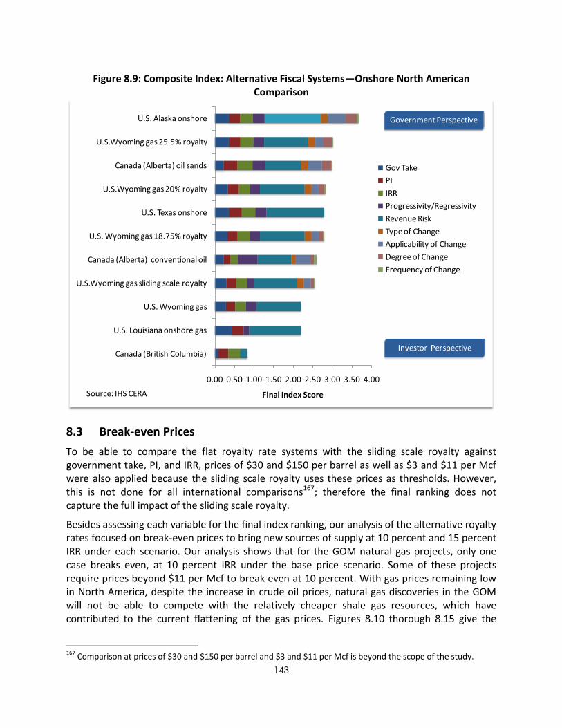
143

Figure 8.9: Composite Index: Alternative Fiscal Systems—Onshore North American Comparison

0.00 0.50 1.00 1.50 2.00 2.50 3.00 3.50 4.00



U.S. Wyoming gas

U.S.Wyoming gas sliding scale royalty



U.S. Texas onshore

U.S.Wyoming gas 20% royalty


U.S.Wyoming gas 25.5% royalty

U.S. Alaska onshore

Final Index Score

Gov Take

PI

IRR


Revenue Risk

Type of Change


Degree of Change

Frequency of Change

Source: IHS CERA



8.3 Break-even Prices

To be able to compare the flat royalty rate systems with the sliding scale royalty against government take, PI, and IRR, prices of $30 and $150 per barrel as well as $3 and $11 per Mcf were also applied because the sliding scale royalty uses these prices as thresholds. However, this is not done for all international comparisons167; therefore the final ranking does not capture the full impact of the sliding scale royalty.

Besides assessing each variable for the final index ranking, our analysis of the alternative royalty rates focused on break-even prices to bring new sources of supply at 10 percent and 15 percent IRR under each scenario. Our analysis shows that for the GOM natural gas projects, only one case breaks even, at 10 percent IRR under the base price scenario. Some of these projects require prices beyond $11 per Mcf to break even at 10 percent. With gas prices remaining low in North America, despite the increase in crude oil prices, natural gas discoveries in the GOM will not be able to compete with the relatively cheaper shale gas resources, which have contributed to the current flattening of the gas prices. Figures 8.10 thorough 8.15 give the

167

Comparison at prices of $30 and $150 per barrel and $3 and $11 per Mcf is beyond the scope of the study.

144

break-even prices for the GOM and Wyoming at 10 and 15 percent IRR.

Figure 8.10: Gulf of Mexico Natural Gas Break-even Prices at 10 Percent IRR

$7

Shelf Gas Field

$9

$7

Shelf Gas Field

$12

$10

Shelf Gas Field

$16

$14

Deepwater Gas Field

$18

$15

Deepwater Gas Field

$20

$16

Deepwater Gas Field

$22

$19

Deepwater Gas Field

$38

$26

$40

$35

$30

$25

$20

$15

$10

$5

$0Shelf Gas

Field

$7

$5

Shelf Gas Field

$9

GOM Representative Gas Fields

Do

llars

per

Mcf

12.5% Royalty

Sliding Scale Royalty

18.75% Royalty

20% Royalty

25% Royalty

Source: IHS CERA

Figure 8.11: Gulf of Mexico Natural Gas Break-even Prices at 15 Percent IRR

9

$15

$50

$45

$40

$35

$20

$30

$25

$45

$30

Shelf Gas Field

$12

Shelf Gas Field

$13

$24

Deepwater Gas Field

$11

Shelf Gas Field

$12

Deepwater Gas Field

$10

Deepwater Gas Field

Shelf Gas Field

$17

Deepwater Gas Field

$24

$29

$24 $11$21$20

Shelf Gas Field

$21

$10

9$5

$0


12.5% Royalty

18.75% Royalty

20% Royalty

25% Royalty

GOM Representative Gas Fields

Do

llars

per

Mcf

Source: IHS CERA At 10 percent IRR Break-even prices for oil fields range from a low of $51 to $136 per barrel

145

under a 12.5 percent royalty rate and $61 to $165 per barrel under a 25 percent royalty rate. At 15 percent IRR, break-even prices range between $71 and $150 per barrel under the 12.5 percent royalty rate and between $84 and $179 per barrel under a 25 percent royalty rate.

Figure 8.12: Gulf of Mexico Crude Oil Break-even Prices at 10 Percent IRR

Deepwater

Oil Field

$61

$51

Deepwater

Oil Field

$63

$53

Deepwater

Oil Field

$69

$56

Deepwater

Oil Field

$74

$64

Deepwater

Oil Field

$85

$71

Shelf

Oil Field

$0

$86

Shelf

Oil Field

$122

$101

Shelf

Oil Field

$165

$139

$100

$80

$60

$40

$20

$180

$160

$140

$120

$102


12.5% Royalty

18.75% Royalty

20% Royalty

25% Royalty

GOM Representative Oil Fields

Do

llars

per

Barr

el

Source: IHS CERA

Figure 8.13: Gulf of Mexico Crude Oil Break-even Prices at 15 Percent IRR

$100

$50

$200

$150

$0Deepwater

Oil Field

$84

$71

Deepwater Oil Field

$82

$70

Deepwater Oil Field

$91

$73

Deepwater Oil Field

$101

$87

Deepwater Oil Field

$113

$95

Shelf Oil Field

$133

$113

Shelf Oil Field

$146

$122

Shelf Oil Field

$179

$150

12.5% Royalty

18.75% Royalty

20% Royalty

25% Royalty


GOM Representative Oil Fields

Do

llars

per

Barr

el

Source: IHS CERA

146

The prospect for natural gas projects in Wyoming is similar to that for the GOM. Except for a few coalbed gas cases, the majority of the projects require rather high natural gas prices to break even at 10 percent IRR. This is largely due to the rather small size of discoveries and very low well productivity.

Figure 8.14: Wyoming Natural Gas Break-even Prices at 10 Percent IRR

$24

$22

$20

$18

$16

$14

$12

$10

$8

$6

$4

$2

$0Gas Field

$1

Coabed Gas Field

$4

$3

Coabed Gas Field

$6

$6

Coabed Gas Field

$7

$6

Coabed Gas Field

$6

$6

Coabed Gas Field

$11

$10

Gas Field

$20

$26

$17

Gas Field

$21

$18

Gas Field

$24

$20

Gas Field

$25

$22


12.5% Royalty

18.75% Royalty

20% Royalty

25% Royalty

Wyoming Representative Gas Fields

Do

llars

per

Mcf

Source: IHS CERA

Figure 8.15: Wyoming Natural Gas Break-even Prices at 15 Percent IRR

$29

$7

Cooalbed Gas Field

$24

$15

$14

Gas Field

$25

$20

$35

$30

$9

$25

$20

$7

$15

$10

Gas Field

$8

Gas Field Cooalbed Gas Field

$0Gas Field

$8

$26

$2

$33

Cooalbed Gas Field

$23

$8

$5

$4

Cooalbed Gas Field

Gas Field Cooalbed Gas Field

$29

$5


12.5% Royalty

18.75% Royalty

20% Royalty

25% Royalty

Wyoming Representative Gas Fields

Do

llars

per

Mcf

Source: IHS CERA

147

8.4 Final Ranking

On a global scale, the introduction of alternative royalty rates higher than the status quo, such as the 20 and 25 percent rates for offshore and 18.75, 20, and 25 percent royalty rates for onshore, place the federal fiscal systems at the top of the ranking chart and contribute to the diminished competitive position. Despite the risk of instability, the introduction of a 12.5 percent royalty rate significantly improves the attractiveness of the GOM fiscal systems. However, this rate reduction may not prove sufficient to bring the GOM marginal fields onstream. Proper comparison of the potential impact of the sliding scale alternative cannot be determined under the price ranges agreed upon with the DOI at the time the study was commissioned. However, when the economics are run under $30 per barrel and $3 per Mcf for the lowest price threshold and $150 per barrel and $11 per Mcf under the highest threshold, the impact on measures of profitability and PI indicate that this alternative is comparable to the 25 percent royalty alternative. When other factors, such as resource potential, potential reduction in revenue collected via signature bonuses and income tax, and the comparable royalty rates for the specific environment are considered, the alternative royalty rates suggested for this study could deter investment and in turn affect timely resource development, which could ultimately lead to reduced federal revenue. Figure 8.16 shows the overall ranking of alternative fiscal systems under the composite index.

Figure 8.16: Composite Index: Alternative Fiscal Systems—Global Ranking

0.00 1.00 2.00 3.00 4.00 5.00

Canada (British Columbia)Poland onshore

Norway offshoreIndonesia coalbed gas

Indonesia conventional gas offshoreAustralia offshore

United Kingdom offshoreAlgeria onshore

India offshoreMalaysia offshoreColombia onshoreGermany onshore

U.S. GOM deepwater 12.5% royaltyAustralia (Queensland) coalbed gas

U.S. Louisiana onshore gasU.S. Wyoming gas

China offshoreU.S. GOM shelf 12.5% royalty

U.S. GOM deepwater sliding scale …U.S.Wyoming gas sliding scale royalty

Canada (Alberta) conventional oilU.S. GOM deepwater

U.S. GOM deepwater 20% royaltyBrazil offshoreU.S. GOM shelf

Libya onshoreAngola offshore

U.S. GOM shelf sliding scale royaltyU.S. GOM shelf 20% royalty

U.S. Wyoming gas 18.75% royaltyU.S. Texas onshore

Kazakhstan offshoreVenezuela conventional gas

U.S.Wyoming gas 20% royaltyU.S. GOM deepwater 25% royalty

Canada (Alberta) oil sandsU.S. GOM shelf 25% royalty

U.S.Wyoming gas 25.5% royaltyRussia onshore

U.S. Alaska onshoreVenezuela heavy oil

Index Score

Gov Take

PI

IRR


Revenue Risk

Type of Change


Degree of Change

Frequency of Change

Source: IHS CERA



148

9. RECOMMENDATION FOR FUTURE UPDATES

One of the findings of the GAO was that the DOI does not routinely evaluate the federal oil and gas fiscal systems as a whole, monitor what other resource owners worldwide are receiving for their energy resources, or evaluate and compare the attractiveness of the United States for oil and gas investment with that of other regions. One of the objectives of this study is to provide recommendations for future updates.

As the GAO pointed out in its report, the purpose of routine evaluation is not only to compare with other jurisdictions to ensure that the U.S. receives a fair return but also to evaluate the attractiveness of the United States for oil and gas investment. The GAO also recognizes that frequent adjustments of fiscal terms are not viewed favorably by industry, especially when they involve increases in royalty rate or other levies.

Countries adopt various approaches when they consider revising fiscal terms or evaluating the competitiveness of their oil and gas sector. These approaches vary widely, and there is no discernible trend. A competitiveness review is effective when

The peer group has been properly identified. A comparison against jurisdictions that do not have any significant production or have not been successful in attracting investments will not provide any useful insights into the true competitive position of a particular oil and gas jurisdiction. In selecting the peer group, it is important that the DOI considers

o whether the jurisdiction competes for investment in the global or regional market

o the type of resources

o the success of the particular jurisdiction in attracting investment

o the types of investors: global versus small regional investors

o common characteristics with respect to

market challenges

cost of development

Actual finding and development costs are being used. Understanding the cost of doing business in the actual jurisdiction is important in being able to make informed decisions. Hypothetical analysis is not very informative for analyzing the attractiveness of a particular jurisdiction. Policy decisions should be based on realistic resource and cost assumptions.

There is a realistic perception of the resource potential. Understanding the resource potential as well as the challenges associated with the recovery of oil and gas is essential in formulating policy. Understanding whether the jurisdiction has reached its maturity is important in making policy decisions. Most countries offer incentives for areas with

149

mature resource potential.

Market analysis is included. Although it is important to compare against other jurisdictions, it is just as important to understand where investments are going, what is driving the low commodity price, and whether the resource under federal land can effectively compete against cheaper resources in the marketplace. Of particular importance for the DOI is to consider the competitiveness of conventional gas discoveries against shale gas development, which is growing rapidly in North America.

With respect to frequency of updates, there is no real recipe as to how often the government should conduct a competitiveness review. Most of the time, such reviews, as is the case with this one, are conducted when the government wants to maintain its competitive position. Often dramatic shifts in market conditions over a sustained period warrant a competitiveness review.

10. CONCLUSION

Government take should not be the only measure to determine attractiveness of the fiscal system. If it is used at all, it should be combined with other measures of profitability, fiscal system flexibility, revenue risk, and fiscal stability in order to properly assess petroleum fiscal systems. Such analysis should be combined with a proper understanding of the resource potential and the relative prospectivity of the federal lands. Fiscal design should be a reflection of the jurisdiction’s relative prospectivity, economic development needs, dependence on hydrocarbon revenues, and environmental protection policies. This study found that all three federal jurisdictions are levying a higher government take than other jurisdictions relative to their remaining recoverable reserve ranking.

From a resource-size perspective, Wyoming conventional resources on federal lands cannot compete with Gulf of Mexico and international jurisdictions selected for this comparative analysis. Because of the size of natural gas fields likely to be discovered in Wyoming, the reserves per new-field wildcat, well productivity, and prevailing natural gas prices in the United States, Wyoming does not appeal to the oil and gas investors likely to invest internationally. In that respect, any ranking of Wyoming in global indexes developed for this study may not be as meaningful, as it is not within its peer group.

When compared with a peer group of North American jurisdictions, Wyoming’s competitive edge is on shaky ground. The province of Alberta and British Columbia are aggressively seeking to attract investment in conventional and unconventional gas resources in two ways: by offering incentives through lower initial royalty rates that encourage development or through net profit royalties that back-end government revenue and allow investors reasonable returns. If shale gas continues to perform better than expected, it could drive the higher-cost resources developed during the high price era that ended in 2008 off the margin. The current royalty rates on federal land do not reflect the maturity of the basins and the high cost of bringing these supplies to market. Although Wyoming may rank more favorably than some of the onshore jurisdictions in North America, its resource base and the high per-unit cost of development of its gas resources make it less appealing to investors, even if paying less on a dollar-per-acre basis for acquisition of acreage in Wyoming compared with Texas or Louisiana.

150

Exploration for and development of natural gas resources in the GOM face the same challenge as the exploration for and development of gas resources in Wyoming. They are a higher-cost alternative to shale gas resources being developed in North America. The current fiscal system on the shelf does not reflect the maturity of the resource. Royalties levied on federal lands in the GOM are the highest among offshore jurisdictions surveyed for this analysis. Therefore they increase the marginal cost of development, discouraging the development of the GOM’s high-cost deep and ultradeep natural gas resources. This is reflected in the rather high ranking of the GOM fiscal systems compared with other offshore and onshore jurisdictions.

The bonus bid system adopted by the federal government is an objective and fair way to allocate acreage. Since the bid value represents the economic rent investors expect to receive from developing the resource, the bonus bid serves as a self-correcting mechanism within the fiscal system. In times of high commodity prices, revenue from bonus bids in Outer Continental Shelf lands has exceeded revenue collected through royalties and rentals combined.

Any increase of the already high royalty rate levied in the GOM will increase the risk of system instability. Any potential gains from the higher royalty rate are likely to be offset by reduced revenue from signature bonuses and the slower pace of leasing.

The 12.5 percent royalty alternative improves the competitive position of the GOM fiscal systems by placing them in the middle of the select peer group. Any of the suggested alternative rates for Wyoming federal lands, however, will deteriorate their competitive position in the market, which is rather weak as it is.

The sliding scale alternatives have been designed to capture the upside, providing no significant relief at the lower end of the scale. The 12.5 percent minimum royalty rate for commodity prices of $30 per barrel and $3 per Mcf is rather high, given that break-even prices at 10 percent discount are in the $70 per barrel range for the GOM jurisdiction.168 The added benefit of flexibility is not really a benefit when the fiscal system is designed simply to capture the upside. Most sliding scale royalties for natural gas adopted in other jurisdictions start at a rate of zero or 2 to 3 percent. A minimum 12.5 percent royalty rate for a sliding scale that exceeds 30 percent at the high end is rather high compared to other offshore jurisdictions.

168

The 12.5 percent royalty rate is the minimum rate established under OCSLA and the Department of Interior cannot lower the threshold without amendment of the statute.

151

BIBLIOGRAPHY

Alberta Department of Energy. “Royalty Information Briefing # 2—What is Fair Share? “ Alberta Royalty Review. 2007.

Alberta Royalty Review Panel. Our Fair Share: Report of the Alberta Royalty Review Panel. 2007.

Alexeev, Michael and Robert Conrad. “The Russian Oil Tax Regime: A Comparative Perspective. Eurasian Geography and Economics 50 no. 3 (2009):93–114.

Anderson, Owen L. “Royalty Valuation: Should Royalty Obligations Be Determined Intrinsically, Theoretically, or Realistically?” Natural Resources Law Journal 37. (1998).

Andrews-Speed, Phillip. “Fiscal Systems for Mining: The Case of Brazil.” Journal of Mineral Policy, Business and Environment 13 no. 2. (1998.

Apps, Peter “Resource nationalism ups political risk premium.” Reuters, November 6, 2009. http://www.reuters.com/article/2009/11/06/us-insurance-political-analysis-idUSTRE5A53DJ20091106, accessed May 2011.

Australian Government Productivity Commission. Review of Regulatory Burden on the Upstream Petroleum (Oil and Gas) Sector. Melbourne: 2009.

Boadway Robin, and Michael Keen. “Theoretical Perspectives on Resource Tax Design. Paper presented at International Monetary Fund Conference on Taxing Natural Resources: New Challenges, New Perspectives, September 25-27, 2008.

BDO USA, LLP. “Volatile Oil and Gas Prices are #1 Risk to U.S. E&P Industry, According to BDO USA Report,” company press release via Business Wire. May 24, 2011. http://www.businesswire.com/news/home/20110524006441/en, accessed May 2011.

Campbell, Rhett G.“Valuing Oil and Gas Assets in the Courtroom.” Presented at the American Institute of Business Law in conjunction with the Oklahoma Bar Review and the Conference on Consumer Finance Law) February 7-8, 2002.

Carroll, Joe., and Jim Polson. “Exxon, Chevron to pay record royalty on Hibernia oil.” Bloomberg, June 16, 2009. http://www.bloomberg.com/apps/news?pid=newsarchive&sid=a4gr_Z.19oYY, accessed May 2011.

Clark, Allan L. “Resource Rent Extraction, Application, Consumption, Investment and Sustainability of Resource-Based Development in Resource-Rich Island Economies.” Presented at UNCTAD Regional Workshop on the Constraints, Challenges, and Prospects for the Commodity-Based Development and Diversification in the Pacific Island Economies on August 18-20, 2001).

Daniel, Philip. et al. “Evaluating Fiscal Regimes for Resource Projects: An Example from Oil Development. Paper presented at International Monetary Fund Conference on Taxing Natural Resources: New Challenges, New Perspectives, September 25-27, 2008.

Derman, Andrew, and Daniel Johnston. “Bonuses Enhance Upstream Fiscal System Analysis. Oil and Gas Journal 51 (1999): 5.

http://www.businesswire.com/news/home/20110524006441/en

http://www.bloomberg.com/apps/news?pid=newsarchive&sid=a4gr_Z.19oYY

152

Dike, Obinna. “Nationalization of Foreign Asset by Hosts State: A Failure of Stabilization Clause?” Center for Energy, Petroleum, Mineral Law and Policy, University of Dundee. 2009.

Fox News. “Brazilian President Signs Law Regulating Pre-salt Oil Reserves.” December 23, 2010http://latino.foxnews.com/latino/money/2010/12/23/brazilian-president-signs-law-regulating-pre-salt-oil-reserves/, accessed May 2011.

Fusco, Leah. “Offshore Oil: An Overview of Development in Newfoundland and Labrador.” http://www.ucs.mun.ca/~oilpower/documents/NL%20oil%207-25-1.pdf, accessed May 2011.

Garnaut, Ross.“Principles and Practice of Resource Rent Taxation.” Australian Economic Review 43 no.4. (2010):347–356.

Goldsworthy, Brenton and Daria Zakharova Evaluation of the Fiscal Regime in Russia and Proposals for Reform. IMF Working Paper 10/33. 2010.

Government of Alberta. Energizing Investment: A Framework to Improve Alberta’s Natural Gas and Conventional Oil Competitiveness. 2010.

Government of Newfoundland and Labrador. Equity, Improved Royalty Regime and Outstanding Local Benefits Highlights of Memorandum of Understanding for Hebron Development. 2007.

Hunter, Tina. Review of the Australian Petroleum Sector: Submission to the Australian Productivity Commission. 2009.

IHS CERA. A Comparison of Fiscal Regimes. http://lba.legis.state.ak.us/aces/doc_log/2007-11-10_cera_a_comparison_of_fiscal_regimes_presented_to_sen_fin.pdf. 2007.

IHS CERA. E&P Fiscal Terms: Larger Pies but Smaller Portions, IHS CERA Decision Brief. 2007.

IHS CERA. A Comparison of Fiscal Regimes: Offshore Natural Gas in Israel. http://www.mof.gov.il/BudgetSite/Reform/Lists/List9/Attachments/43/novelEnergy_4.pdf. 2010.

International Energy Agency. The Impact of the Financial and Economic Crisis on Global Energy Investment. International Energy Agency Background Paper for the G8 Energy Minister’s Meeting. May 2009.

Johnston, Daniel. “Changing Fiscal Landscape.” Journal of World Energy Law and Business 1 no. 1. 2008.

Johnston, Daniel. “Current Developments in Production Sharing Contracts and International Concerns: Retrospective Government Take—Not a Perfect Statistic.” Petroleum Accounting and Financial Management. Journal 21. No. 2 (2002), 101–108.

Kaiser, Mark J. and Allan, G. Pulsipher. Fiscal System Analysis: Concessionary and Contractual Systems Used in Offshore Petroleum Arrangements. U.S. Department of the Interior, Minerals Management Service, Gulf of Mexico OCS Region, New Orleans, La. OCS Study MMS 2004-016

Kepes, Jerry, Barry Rogers, and Pedro van Meurs. “Gas Prices, Other Factors Indicate Changes in North American Shale Play Fiscal Systems.” Oil and Gas Journal 109 (2011).

Land, Bryan. “Capturing a Fair Share of Fiscal Benefits in the Extractive Industries.”



http://www.ucs.mun.ca/~oilpower/documents/NL%20oil%207-25-1.pdf



http://www.mof.gov.il/BudgetSite/Reform/Lists/List9/Attachments/43/novelEnergy_4.pdf

153

Transnational Corporations Journal 18 no. 1 (2009): 157-174.

Locke, Wade. “Is Newfoundland and Labrador getting its fair share?” Newfoundland Quarterly 99. (2007): 3.

Mariano, Jacqueline and Emilio La Rovere. “Oil and Gas Exploration and Production Activities in Brazil: The Consideration of Environmental Issues in the Bidding Rounds Promoted By the National Petroleum Agency.” Energy Policy 35 (2007): 2899–2911.

Nakhle, Carole Petroleum Taxation: Sharing the oil wealth: A study of petroleum taxation yesterday, today and tomorrow. New York: Routledge, 2008.

National Petroleum Council. Facing the Hard Truths About Energy: A Comprehensive View to 2030 of Global Oil and Natural Gas. 2007.

Opaluch, James, J., et al. Policies to affect the pace of leasing and revenues in the Gulf of Mexico. U.S. Department of the Interior, Bureau of Ocean Energy Management, Regulation and Enforcement, Gulf of Mexico OCS Region, New Orleans, LA. OCS Study BOEMRE 2011-013. 2009.

Pate, Thomas J. “Evaluating stabilization clauses in Venezuela's strategic association agreements for heavy-crude extraction in the Orinoco Belt: The return of a forgotten contractual risk reduction mechanism for the petroleum industry.” University of Miami Inter-American Law Review 40 (2009): 347.

PricewaterhouseCoopers. “The Economic Impacts of the Oil and Natural Gas Industry on the U.S. Economy: Employment, Labor Income and Value Added” (September 2009).

Randall, Stephen and Jillian Dowding. “Colombia Current and Future Political, Economic and Security Trends.” Canadian Defense and Foreign Affairs Institute. (December 2006)

Shulga, Arina. “Foreign investment in Russia’s oil and gas: Legal framework and lessons for the future.” University of Pennylvania Journal of International Economic Law 22 (2001): 1067-1103.

Sierra Systems. Project committee final report to the Alberta Department of Energy on Alberta’s natural gas and conventional oil competitiveness. (2010): Appendix B-12.

Smith, James L.,Daniel R. Siegel, and C. S. Agnes Cheng. “Failure of the net profit sharing experiment for offshore petroleum resources.” The Review of Economics and Statistics 70 no. 2. (May 1998), 199–206.

Storting. An Industry for the Future—Norway’s Petroleum Activities. White Paper 28. 2010.

Sunley, Emil M., Thomas Baunsgaard, and Dominique Simard. “Revenue from Oil and Gas Sector: Issues and Country Experience.” Background Paper prepared for the IMF Conference on Fiscal Policy Formulation and Implementation in Oil Producing Countries, June 5–6, 2002. World Bank.

Tordo, Silviana. “Fiscal Systems for Hydrocarbons: Design Issues.” World Bank Working Paper No. 123. (2007).

Tordo, Silviana, David Johnston, and Daniel Johnston. “Countries’ Experience with the Allocation of Petroleum Exploration and Production Rights: Strategies and Design Issues.”

154

World Bank Working Paper No. 179.

United Nations Conference on Trade and Development. “Administration of Fiscal Regimes for Petroleum Exploration and Development.” United Nations Conference on Trade and Development Advisory Service on Investment and Training Advisory Studies. Geneva: June 1996.

U.S. Government Accountability Office. The Federal System for Collecting Oil and Gas Revenues Needs Comprehensive Reassessment. Report to Congressional Requesters GAO-08-691 (2008).

U.S. Departments of Interior, Agriculture, and Energy. Inventory of Onshore Federal Oil and Natural Gas Resources and Restrictions to Their Development, Phase III Inventory—Onshore United States (Washington, DC: 2008).

Van Meurs Corporation. Comparative analysis of fiscal terms for Alberta oil sands and international heavy and conventional oils (2007).

Van Meurs, Pedro. “Preliminary Fiscal Evaluation of Alberta Oil Sands Terms,” presented to the Alberta Departmern of Energy, April 12, 2007.

Waelde, Thomas W. and George Ndi. “Stabilizing International Investment Commitments: International Law Versus Contract Interpretation.” Texas International Law Journal 31 no. 2 (1996), 216.

155

APPENDIX I—FIELD SELECTION CRITERIA

To provide “apples to apples” comparison of the fiscal systems, as well as the opportunities for prospective investors in each of the selected jurisdictions, the study relies on economic modeling of actual fields discovered during the 2000–2010 period in the respective jurisdiction, with 2010 exploration and production costs applicable in each region. An exception was made in the case of Alaska North Slope, where the analysis included a couple of fields that were discovered prior to 2000 but had not been developed yet owing to their remoteness from infrastructure and commodity markets. A total of 153 exploration and development cost models representing 124 conventional field developments and 29 unconventional oil and gas projects were selected for this comparative review. In jurisdictions with potential for oil and gas investments, three oil and three gas fields were selected, whereas in other jurisdictions where either oil or gas was the predominant fuel or they were active in conventional as well as unconventional resource development, the fields selected were either all gas fields (as in the case of Wyoming, where conventional and unconventional gas models were developed) or all oil fields (as in the case of Alberta, where three conventional oil fields and three oil sands projects were modeled).

The conventional fields selected for this study are for the most part representative of small, medium, and large field sizes for oil and gas in the respective jurisdiction, based on the pool of discoveries made in the past ten years. However, owing to the relatively small size of discoveries in various oil and gas jurisdictions, the selection sometimes weighed heavily on the larger sized fields.169 As a result 50 percent of the conventional fields selected fall in the 80–100 percent rank of discoveries of the past decade in the respective petroleum jurisdictions. The analysis shows that even with this field selection that is skewed toward fields ranking in the top 40 percent, less than 50 percent of the fields yield desirable rates of return under a high oil price environment. Figure I.I shows the number of fields per distribution rank.

169In a number of jurisdictions, such as the U.S. Gulf of Mexico Shelf, Poland, Russia, and Australia, the smaller field sizes fall above the 50 percent distribution rank. This is due to the rather large number of fields falling within the small fields group (80–90 percent of the fields in some cases). The sizes selected represent the average small fields for the respective jurisdictions. Thus, for example, in Russia the small gas fields ranged between 2 billion cubic feet (Bcf) and 84 Bcf of recoverable reserves. The representative small field selected was 34 Bcf. The medium-sized field usually represents the arithmetic mean of all discoveries in the respective jurisdiction despite the distribution rank.

156

Figure I-I: Selected Fields

0

5

10

15

20

25

30

35

40

100 90-99 80-89 70-79 60-69 50-59 40-49 30-39 0-29

No

. o

f C

on

ven

tio

nal

Fie

lds

Distribution Percentile

Gas

Oil

Source: IHS CERA

50% of fields - >80% rank

Unlike conventional oil and gas resources where the areal extent of fields is such that a single company or group of companies can develop them under a single concession or PSA, the areal extent of unconventional plays such as extra heavy oil, oil sands, coalbed gas, and shale gas, for example, is so vast that a single play is covered by numerous licenses and leases. The size of a project in such a case would depend to a large extent on the ability to acquire rights over significant acreage. For this same reason, the unconventional oil and gas developments that were selected are not accounted for in the field distribution analysis. However, they represent typical projects that have been undertaken or are currently under way in the respective jurisdictions.

The development concepts represent typical developments for each environment, taking into account distance from existing facilities and infrastructure, technological challenges associated with deepwater and ultra-deepwater exploration and development, arctic environment, reservoir pressure, well flow rates where available, water and reservoir depth, and risk premiums applicable in each environment. Such concepts do not provide contingencies for human error, project delays, or delayed development owing to lack of a market or portfolio optimization on the part of operators. They do, however, take into account the exploration success rate in each environment, which is reflected in the number of exploratory wells included in each model, as well as any payments associated with award of acreage.

157

Table I-I: Fiscal Systems and Resource Type

COUNTRY FISCAL SYSTEM RESOURCE

Conventional Oil

Conventional Gas

Unconventional Oil

Unconventional Gas

On

sho

re

Off

sho

re

On

sho

re

Off

sho

re

On

sho

re

Off

sho

re

On

sho

re

Off

sho

re

Algeria Concessionary √ - √ - - - - -

Angola PSA - √ - √ - - - -

Australia Federal—Concessionary - - - √ - - - -

Queensland—Concessionary - - - - - - √ -

Brazil Concessionary - √ - √ - - - -

Canada Alberta Conventional Oil–Concessionary

√ - - - - - - -

Alberta Oil Sands—Concessionary - - - - √ - - -

British Columbia Shale Gas—Concessionary

- - - - - - √ -

China PSA - √ - √ - - - -

Colombia Concessionary √ - √ - - - - -

Germany Concessionary - - - - - - √ -

India PSA - √ - √ - - - -

Indonesia Conventional PSA - - - √ - - - -

CBG PSA - - - - - √ -

Kazakhstan Concessionary - √ - - - - - -

Libya PSA √ - √ - - - - -

Malaysia PSA - √ - √ - - - -

Norway Concessionary - √ - √ - - - -

Poland Concessionary - - √ - - - √ -

158

COUNTRY FISCAL SYSTEM RESOURCE

Conventional Oil

Conventional Gas

Unconventional Oil

Unconventional Gas

On

sho

re

Off

sho

re

On

sho

re

Off

sho

re

On

sho

re

Off

sho

re

On

sho

re

Off

sho

re

Russia Concessionary √ - √ - - - - -

United Kingdom

Concessionary - √ - √ - - - -

United States DW GOM—Concessionary - √ - √ - - - -

Shelf GOM—Concessionary - √ - √ - - - -

Alaska—Concessionary √ - √ - - - - -

Louisiana—Concessionary - - - √ - - √ -

Texas—Concessionary √ - √ - - - - -

Wyoming Federal—Concessionary - - √ - - - √ -

Venezuela Heavy Oil—Concessionary - - - - √ - - -

Gas—Concessionary - - √ - - - - -

159

1. Selection of Fields on Federal Lands

Since the focus of the study is to compare U.S. federal oil and gas fiscal systems with other jurisdictions, as well as to analyze and compare alternative fiscal systems resulting from proposed fixed and sliding scale royalties, ten field development concepts were modeled for each of the federal fiscal systems.

With respect to the Gulf of Mexico, the selection process focused not just on the size of the fields, but also on the water depth and formation depth in order to include deepwater as well as deep formations in line with the trend of proved reserves in the region. Data from BOEM show that shallow-water proved gas reserves in the GOM in 2009 make up 50 percent of the proved gas reserves of the region, and proved oil reserves make up 16 percent of the oil reserves in the region.

Figure I-II: Gulf of Mexico Proved Gas Reserves

-

2,000

4,000

6,000

8,000

10,000

12,000

14,000

16,000

18,000

20,000

2005 2006 2007 2008 2009

Pro

ved

Gas

Re

serv

es

(Bcf

)

Year

Shallow Water Deep Water Ultradeep Water

Source: BOEMRE

This greater propensity for gas discoveries on the shelf is also reflected in the field selection for this study, which consists of seven gas fields and three oil fields. In order to represent the full spectrum of discoveries in shallow water in the GOM as well as to examine the impact, if any, of the royalty relief mechanisms in place, a couple of deep gas and ultradeep gas discoveries, which qualify for royalty relief when the natural gas price is below a certain threshold, were modeled. The field sizes for shallow water in the Gulf of Mexico reflect the maturity of the jurisdiction. The analysis shows that even the top ranked discoveries of the past decade do not reach the 15 percent rate of return threshold under current cost and commodity prices.

160

Figure I-III: Gulf of Mexico Proved Oil Reserves

-

500

1,000

1,500

2,000

2,500

3,000

3,500

4,000

4,500

5,000

2005 2006 2007 2008 2009

Pro

ve

d O

il R

ese

rve

s (M

MB

bl)

Year

Shallow Water Deep Water Ultradeep Water

Source: BOEMRE

Figure I-IV: Gulf of Mexico Shelf Discovered Fields (2000–2010)

0

20

40

60

80

100

120

140

160

180

200

0% 25% 50% 75% 100%

Mill

ion

Ba

rre

ls O

il Eq

uiv

ale

nt

Distribution Rank

16 Oil Fields - 95 Gas Fields

Other Gas Other Oil Selected Gas Selected Oil

Source: IHS CERA

161

Although there is no separate fiscal system governing deepwater and ultra-deepwater exploration and production in the Gulf of Mexico, the fields selected for deepwater GOM include discoveries in deepwater as well as ultra-deepwater ranging from 2,400 feet to 8,300 feet, with 80 percent of the fields being located below 5,000 feet of water depth and formation depth ranging from 7,600 feet to 35,000 feet.170 Unlike the shelf fields, the deepwater GOM fields selected represent a wider distribution within the pool of discoveries made in the past ten years. However, analysis shows that fields falling below the 75 percent rank do not reach the 15 percent rate of return threshold under the current cost and price environment.

Figure I-V: Gulf of Mexico Deepwater Field Discoveries (2000–2010)

0

100

200

300

400

500

600

700

0% 25% 50% 75% 100%

Mill

ion

Bar

rels

Oil

Equ

ival

ent

Distribution Rank



Source: IHS CERA

Unlike the GOM region, which shows relatively high levels of activity in terms of number of discoveries made during the 2000–10 period, the conventional discoveries made on federal lands in Wyoming are dramatically lower in number as wells as in reserve size. A large share of current development and production in Wyoming is on fields discovered before the study’s ten-year window; however, the limited number of recent discoveries and the size of recoverable reserves associated with such discoveries is a better indication of future prospectivity of conventional resources of the jurisdiction.

170

According to BOEMRE, ultra-deepwater is 5,000 feet of water or greater.

162

The size of reserves and well productivity is such that four out of five conventional fields selected are not economic under any price scenario. Coalbed gas, on the other hand, appears to offer marginally better investment opportunities on federal lands in Wyoming under certain gas and price assumptions. Five different projects representative of coalbed gas opportunities offered in Big George, East Green River, and Wyodak were modeled for the purpose of this study.

Figure I-VI: Wyoming Federal Lands Fields Discovered (2000–2010)

0

1,000

2,000

3,000

4,000

5,000

6,000

0% 25% 50% 75% 100%

Tho

usa

nd

Ba

rre

ls O

il E

qu

ival

ent

Distribution Rank



Source: IHS CERA

Wyoming conventional fields were modeled from IHS well-based data. Although the fields selected represent ones with wells drilled on federal lands, such fields were modeled as a whole, i.e., wells located outside the federal lands jurisdiction were taken into account in the model.

163

Table I-II: U.S. Wyoming Coalbed Gas Projects


Field Recoverable Reserves (MMcf) Daily Production (Mcf per day)

Wyoming CBG 1 820,000.00 150

Wyoming CBG 2 630,000.00 150

Wyoming CBG 3 230,000.00 50

Wyoming CBG 4 160,000.00 20

Wyoming CBG 5 110,000.00 30

Source: IHS CERA

2. Selection of Fields in Other Jurisdictions

Figure I-VII: Algeria Onshore Discoveries (2000–2010)

0

50

100

150

200

250

300

0% 25% 50% 75% 100%

Mill

ion

Bar

rels

Oil

Equ

ival

ent

Distribution Rank



Source: IHS CERA

164

Figure I-VIII: Angola Offshore Discoveries (2000–2010)

0

50

100

150

200

250

300

350

0% 25% 50% 75% 100%

Mill

ion

Ba

rre

ls O

il E

qu

iva

len

t

Distribution Rank



Source: IHS CERA

Figure I-IX: Australia Offshore Discoveries (2000–2010)

0

500

1,000

1,500

2,000

2,500

3,000

3,500

4,000

0% 25% 50% 75% 100%

Mill

ion

Ba

rre

ls O

il Eq

uiv

ale

nt

Distribution Rank



Source: IHS CERA

165

Table I-III: Australia (Queensland) Coalbed Gas Fields Modeled

Field Gas (MMcf)

CBG 1 2,490,000.00

CBG 2 694,000.00 CBG 3 2,222,000.00

Source: IHS CERA

Figure I-X: Brazil Offshore Discoveries (2000–2010)

0

1,000

2,000

3,000

4,000

5,000

6,000

7,000

0% 25% 50% 75% 100%

Mill

ion

Ba

rre

ls O

il Eq

uiv

ale

nt

Distribution Rank



Source: IHS CERA

166

Figure I-XI: Canada (Alberta) Discoveries (2000–2010)

0

20

40

60

80

100

120

0% 25% 50% 75% 100%

Mill

ion

Ba

rre

ls O

il Eq

uiv

ale

nt

Distribution Rank



Source: IHS CERA

Table I-IV: Canada (Alberta) Oil Sands Modeled

Field Reserves (million barrels)

Case 1—SAGD w/ Upgrader 2,165.00

Case 2—SAGD w/o Upgrader 2,165.00

Case 3—Mining w/ Upgrader 1,040.00

Source: IHS CERA

Table I-V: Canada (British Columbia) Shale and Tight Gas Plays Modeled

Field Gas (MMcf)

Case 1–shale 500 MMcfd 4,210,000.00 Case 2–tight sands 500 MMcfd 2,260,000.00 Case 3–shale 400 MMcfd 2,410,000.00

Source: IHS CERA

167

Figure I-XII: China Offshore Discoveries (2000–2010)

0

200

400

600

800

1,000

1,200

1,400

1,600

1,800

2,000

0% 25% 50% 75% 100%

Mill

ion

Ba

rre

ls O

il Eq

uiv

ale

nt

Distribution Rank



Source: IHS CERA

Figure I-XIII: Colombia Onshore Discoveries (2000–2010)

0

50

100

150

200

250

300

0% 25% 50% 75% 100%

Mill

ion

Bar

rels

Oil

Equ

ival

ent

Distribution Rank

92 Oil Field - 16 Gas Fields


Source: IHS CERA

168

Table I-VI: Germany Shale Gas Models

Field Gas (MMcf)

Case 1—350 MMcf per day 2,270,000.00

Case 2—150 MMcf per day 910,000.00


Source: IHS CERA

Figure I-XIV: India Offshore Discoveries (2000–2010)

0

200

400

600

800

1,000

1,200

1,400

0% 25% 50% 75% 100%

Mil

lio

n B

arr

els

Oil

Eq

uiv

ale

nt

Distribution Rank



Source: IHS CERA

169

Figure I-XV: Indonesia Offshore Discoveries (2000–2010)

0

200

400

600

800

1,000

1,200

1,400

1,600

1,800

2,000

0% 25% 50% 75% 100%

Mil

lio

n B

arr

els

Oil

Eq

uiv

ale

nt

Distribution Rank



Source: IHS CERA

Table I-VII: Indonesia Coalbed Gas Fields Modeled

Field Gas (MMcf)

CBG 2,490,000.00

CBG 694,000.00

CBG 2,222,000.00

Source: IHS CERA

170

Figure I-XVI: Kazakhstan Offshore Discoveries (2000–2010)

0

2,000

4,000

6,000

8,000

10,000

12,000

14,000

16,000

18,000

20,000

0% 25% 50% 75% 100%

Mill

ion

Bar

rels

Oil

Equ

ival

ent

Distribution Rank



Source: IHS CERA

Figure I-XVII: Libya Onshore Discoveries (2000–2010)

0

100

200

300

400

500

600

700

800

900

1,000

0% 25% 50% 75% 100%

Mil

lio

n B

arr

els

Oil

Eq

uiv

ale

nt

Distribution Rank



Source: IHS CERA

171

Figure I-XVIII: Malaysia Offshore Discoveries (2000–2010)

0

100

200

300

400

500

600

700

0% 25% 50% 75% 100%

Mill

ion

Bar

rels

Oil

Equ

ival

ent

Distribution Rank



Source: IHS CERA

Figure I-XIX: Norway Discoveries (2000–2010)

0

50

100

150

200

250

300

0% 25% 50% 75% 100%

Mill

ion

Bar

rels

Oil

Equ

ival

ent

Distribution Rank



Source: IHS CERA

172

Figure I-XX: Poland Conventional Field Discoveries (2000–2010)

0

10

20

30

40

50

60

70

80

0% 25% 50% 75% 100%

Mil

lio

n B

arre

ls O

il E

qu

ival

en

t

Distribution Rank



Source: IHS CERA

Table I-VIII: Poland Shale Gas Projects

Field Gas (MMcf)

Case 1—200 MMcf per day 1,180,000.00

Case 2—160 MMcf per day 1,030,000.00


Source: IHS CERA

173

Figure I-XXI: Russia Onshore Discoveries (2000–2010)

0

50

100

150

200

250

300

0% 25% 50% 75% 100%

Mil

lio

n B

arr

els

Oil

Eq

uiv

ale

nt

Distribution Rank



Source: IHS CERA

Figure I-XXII: United Kingdom Offshore Discoveries (2000–2010)

0

100

200

300

400

500

600

700

800

0% 25% 50% 75% 100%

Mil

lio

n B

arr

els

Oil

Eq

uiv

ale

nt

Distribution Rank



Source: IHS CERA

174

Table I-IX: U.S. Alaska Selected Fields

Field Type Gas (MMcf) Oil (barrels)

Gas 2162 189.73

Gas 209 -

Gas 30 20.6

Oil 862 621.59

Oil 370 102.34

Oil - 55.71

Source: IHS CERA

Figure I-XXIII: U.S. Louisiana Onshore Discoveries on State Land (2000–2010)

0

10

20

30

40

50

60

0% 25% 50% 75% 100%

Mil

lio

n B

arr

els

Oil

Eq

uiv

ale

nt

Distribution Rank



Source: IHS CERA

Table I-X: U.S. Louisiana Shale Gas Projects Modeled

Field Gas (MMcf)

Case 1 3,830,000

Case 2 2,270,000

Case 3 2,000,000

Source: IHS CERA

175

Figure I-XXIV: U.S. Texas Onshore Discoveries on State Land (2000–2010)

0

50

100

150

200

250

300

350

400

450

0% 25% 50% 75% 100%

Mill

ion

Ba

rre

ls O

il E

qu

iva

len

t

Distribution Rank



Source: IHS CERA

Figure I-XXV: Venezuela Onshore Discoveries (2000–2010)

0

2

4

6

8

10

12

14

16

0% 25% 50% 75% 100%

Mill

ion

Bar

rels

Oil

Equ

ival

ent

Distribution Rank



Source: IHS CERA

176

Table I-XI: Venezuela Extra Heavy Oil Projects

Field Oil (million barrels)

Case 1 2,558.00

Case 2 2,165.00

Case 3 2,165.00

Source: IHS CERA

177

APPENDIX II—ASSUMED FISCAL TERMS

A. Model Assumptions

Fields are modeled as stand-alone projects

Prices are netted back at the wellhead o Exception: In international models where the upstream operator is responsible

for building the connecting pipelines to the delivery point (main transportation and transmission lines or liquefied natural gas [LNG] terminal), the cost of connecting to such facilities is taken into account. The respective transportation and processing costs are allowed as deductions for royalty purposes.

The model uses nominal, rather than effective, tax rates. Appropriate deductions and applicable allowances and credits are applied. Depending on the jurisdiction they include but are not limited to o Depreciation of capital expenditure

Straight line Declining balance Appropriate uplifts171

o Allowable deductions Royalty Operating expenses Other taxes Depletion allowances Small field allowances Carry forward and back of losses

o Tax Incentives—credits, holidays

Economics is run in constant dollars

10 percent real discount rate applied

Undiscounted government take

Economic limit is applied on all projects172

No reserve growth factor is taken into account

Projects are risked by accounting for unsuccessful exploratory wells

Input costs from QUE$TOR models include capital expenditure distinguishing between tangible and intangible operating expenses—identifying separately any transportation or processing costs—and the cost of decommission and abandonment of facilities.

171

Accelerated depreciation. 172

When the operating costs of a field exceed gross revenues associated with that field, the field is no longer considered an asset and is said to have achieved its economic limit.

178

B. Fiscal Systems

1. ALGERIA ONSHORE

Various fiscal systems apply in Algeria depending on the time the contract was awarded and the location of the acreage. This study analyzes the terms currently in force for Zone D onshore, introduced by the 2005 Hydrocarbon Law as amended by subsequent legislation.

Table II-I: Algeria Assumed Terms

FISCAL SYSTEM Algeria—2005 Hydrocarbons Law Concessionary Terms for Zone D

BONUSES Signature bonus of US$1 million

RENTAL 8,000–32,000 dinars(DA) per km2

STATE PARTICIPATION 51 percent carried to discovery with repayment of past costs without interest

ROYALTY 12.5–23 percent of gross revenue tied to average daily production

INCOME TAX 30 percent of revenue less deductions and depreciation

ADDITIONAL PROFITS TAX Levied on revenue less deductions and depreciation (including 20 percent uplift): 30–70 percent tied to cumulative production value

BONUSES AND OTHER PAYMENTS

A biddable signature bonus is payable. US$1 million has been assumed here. The signature bonus is not allowable as a deduction against income tax and Petroleum Revenue Tax.

The 2005 Hydrocarbons Law does not prescribe for payment of production bonuses or a training fee, and none have been assumed here.

RENTAL

Rentals may be paid in U.S. dollars or Algerian dinars at the exchange rate in force on the payment date. They vary by zone. Rental rates assumed here are those applicable to Zone D, expressed in dinars per square kilometer.

Table II-II: Algeria Rental

Contract Location

Exploration phase Retention Period

(DA/km2)

Development and

Production Phase

(DA/km2)

Years 1 to 3

(DA/km2)

Years 4 and 5

(DA/km2)

Years 6 and 7

(DA/km2)

Zone D 8,000 12,000 16,000 800,000 32,000

179

The fiscal system also includes a range of minor taxes as follows:

land tax on assets other than exploitation assets

a 1 percent assignment tax

a gas flaring tax of 8,000 dinars per 1,000 normal cubic meters

water tax at the rate of 80 dinars per cubic meter of drinkable or irrigation water used in enhanced recovery operations

a tax on the "use, transfer, or assignment" of greenhouse gas emissions credits

The above-mentioned fees and taxes have not been modeled here.

STATE PARTICIPATION

Sonatrach, the NOC, takes a participating interest of at least 51 percent in all exploration and production contracts. Sonatrach is required to pay its participating interest share of all investment and exploitation costs related to the development plan approved by Alnaft.173 Sonatrach's participating interest of 51 percent carried to commercial discovery with repayment of past exploration costs without interest has been assumed here.

ROYALTY Royalty is payable on a sliding scale linked to daily production rates and varying with the location of the contract area. Legislation specifies minimum royalty rates.174 Royalty rates may be bid at higher levels where Alnaft, the competent authority, decides that royalty is the principal criterion for allocation of acreage. Minimum royalty rates for Zone D have been assumed.

Table II-III: Algeria Oil and Gas Royalty Rates

ROYALTY UNDER 2005 HYDROCARBONS LAW—ZONE D

Increment of Average Daily Production

Minimum Royalty Rate (percent) Oil (million barrels per day [mbd]))

Gas (million cubic feet [MMcf] per day)

0–20 0–120 12.5

20–50 120–300 20.0

50–100 300–600 23.0

> 100* > 600 20.0

*When average daily production is < 100 million barrels oil equivalent (MMboe) per day, royalty is levied on an incremental basis. When average daily production is > 100 MMboe per day, royalty is levied on total production.

INCOME TAX

Investors are subject to tax on their profits levied at a fixed rate of 30 percent.175 Income tax is

173 Ordinance No. 06-10 of July 29, 2006 (2006 AHL), Art. 2(32), 2(48). 174 2005 Hydrocarbon Law, Art. 33, 83, 85. 175 2005 Hydrocarbon Law, Art. 83, 88; 2006 AHL Art. 2(88).The generally applicable corporate income tax is 25 percent; however, the Hydrocarbon Law sets the corporate income tax for upstream investments at 30 percent.

180

levied on gross revenue less royalty, petroleum revenue tax, abandonment costs, operating costs, exploration costs, intangible development costs, depreciation of development drilling costs over eight years straight-line, and depreciation of operational facilities and pipelines over ten years straight-line.

ADDITIONAL PROFITS TAX

Investors are subject to Petroleum Revenue Tax (PRT), levied on gross revenue less royalty, abandonment costs, and depreciation of capital costs over eight years straight-line with a 20 percent uplift.

Table II-IV: Algeria Petroleum Revenue Tax

PETROLEUM REVENUE TAX UNDER THE 2005 HYDROCARBONS LAW

Cumulative Production (PV) Petroleum Revenue Tax Rate (percent)

Threshold (billions of Algerian Dinars)

First (S1) PV < 70 30

70 < PV < 385 40 x [(PV—S1)/(S2—S1)] + 30

Second (S2) > 385 70

2. ANGOLA—OFFSHORE

The terms used for this study relate to the latest model contract released in 2008.

Table II-V: Angola Assumed Terms

FISCAL SYSTEM Angola—2008 Model PSA Terms Offshore (Ultra-deepwater > 1,000 m)

BONUSES Signature bonus of US$20–$400 million

OTHER PAYMENTS Annual training fee of US$200,000 during exploration and development periods and US$0.15 per barrel (US$0.025 per Mcf) during production period

Social contribution of US$4 million at project start-up

STATE PARTICIPATION 20 percent carried through to discovery with repayment of past costs

ROYALTY None

COST RECOVERY From 50 percent of gross revenue

PROFIT SHARING 20–70 percent based on a sliding scale linked to IRR

INCOME TAX 50 percent of profit share

181


Bonuses

A negotiable signature bonus is payable for acquisition of acreage. Bonuses ranging between US$20 million and US$400 million have been assumed here. The bonuses are a nonrecoverable cost for profit-sharing purposes.

Training Fee

The contractor is required to contribute a negotiable amount toward the training of Angolan staff; indicative annual amounts of US$200,000 during exploration and development periods and US$0.15 per barrel (US$0.025 per Mcf) during the production period have been assumed here. The training fee is a recoverable cost for profit-sharing purposes.

Social Contribution

Upon signing the contract, the contractor is required to make a negotiable contribution for social projects; US$4 million has been assumed here. Social contribution is a nonrecoverable cost for profit-sharing purposes.

STATE PARTICIPATION

Participation of Sonangol, the NOC, at 20 percent carried through to commercial discovery with repayment of the exploration costs from Sonangol's cost recovery petroleum has been assumed.

ROYALTY

None has been assumed. The 2004 Petroleum Tax Law makes provisions for the payment of a tax on production (i.e., royalty) at a rate of 20 percent, which may be reduced to 10 percent for certain areas at Sonangol's discretion. However, petroleum produced under the terms of the production sharing contract is specifically exempt from this tax.176

COST RECOVERY

Costs are recovered from 50 percent of gross revenue in the following order: operating costs, development costs, and exploration costs. Operating costs and exploration and appraisal (E&A) costs are expensed and recovered immediately; development costs, including a 20 percent uplift, are capitalized and recovered over four years on a straight-line basis starting from the commencement of commercial production. Losses may be carried forward indefinitely, but not beyond the duration of the contract.

PROFIT SHARING

Production remaining after cost recovery is assumed to be shared between Sonangol and the contractor on a scale linked to after-tax nominal internal rate of return (IRR) as follows:

176

2004 Petroleum Tax Law, Art. 12.4. All contracts awarded in Angola are production sharing agreements.

182

Table II-VI: Angola Contractor Profit Share

PROFIT SHARING

IRR (percent) Contractor's Profit Share (percent)

≤ 10 70

10–12.5 55

12.5–17.5 45

17.5–20 30

≥ 20 20

INCOME TAX

Income tax is levied on the contractor's profit share at a rate of 50 percent.177 Since the value of cost recovery is not included in the taxable income, there are effectively no deductions for tax purposes. The 2004 Petroleum Tax Law also provides for petroleum transaction tax levied at a rate of 70 percent on taxable revenue. However, petroleum operations conducted under a production sharing contract are exempt from this tax.178

3. AUSTRALIA—OFFSHORE FEDERAL JURISDICTION

Table II-VII: Australia Federal Assumed Terms

FISCAL SYSTEM Australia—Offshore Concessionary Terms (except Northewest Shelf) beyond 3 mile limit

BONUSES None

RENTALS Exploration: A$1,135 per year; Production: A$20,460 per year

ROYALTY None

INCOME TAX Levied on gross revenue less deductions and depreciation. The income tax rate is 30 percent.

ADDITIONAL PROFITS TAX Known as petroleum resource rent tax (PRRT) and levied on a project's taxable profit (project revenue less project E&A costs, project development costs, and exploration costs of other related PRRT projects). The PRRT rate is 40 percent.


There is no provision for the payment of a signature bonus, discovery bonus, or production bonuses. Annual rentals are payable for E&P rights. For the 2010 acreage release, the following area rentals (inclusive of GST) were applied:

177

2004PTL , Art. 19, 41(b). The general corporate income tax rate is currently 35 percent. 178

2004 PTL Art 44.

183

Table II-VIII: Australia Offshore Rentals

Type of Right Rental (A$ per year) Exploration Permit 1,135 minimum per block Production License 20,460 per block

STATE PARTICIPATION

None.

ROYALTY

None.

PETROLEUM RESOURCE RENT TAX

Petroleum Resource Rent Tax (PRRT) applies to all petroleum projects in waters beyond the 3 mile territorial sea limit except for certain designated licenses. PRRT is levied on net cash flow once operating and development costs have been deducted and carried forward with interest. The rate of PRRT is 40 percent.

INCOME TAX

Income tax is levied at 30 percent on gross revenue less E&A costs, operating costs, royalty, crude oil excise, petroleum resource rent tax, and depreciation of development costs on either a straight-line or declining balance basis over the asset life; eight years on a straight-line basis is assumed here. Deductions and depreciation commence from the year of expenditure. Losses may be carried forward indefinitely.

4. AUSTRALIA—QUEENSLAND COALBED GAS

Table II-IX: Australia—Queensland Assumed Terms

FISCAL SYSTEM Australia—Queensland Concessionary Terms

BONUSES None

RENTALS Exploration: A$2.35 per km2; Production: A$119.15 per km2

ROYALTY 10 percent

INCOME TAX Levied on gross revenue less deductions and depreciation. The income tax rate is 30 percent

ADDITIONAL PROFITS TAX Not currently applicable. To be applied from July 1, 2012.


There is no provision for the payment of a signature bonus, discovery bonus, or production bonuses. Annual rentals are payable for E&P rights. The following rental payments apply to E&P

184

rights in Queensland:

Table II-X: Australia—Queensland Rentals

Type of Right Rental (A$ per km2)

Exploration Permit 2.35 Production License 199.15

STATE PARTICIPATION

None.

ROYALTY

10 percent payable to the government of Queensland.

INCOME TAX

Federal income tax is levied at 30 percent on gross revenue less E&A costs, operating costs, royalty, crude oil excise, petroleum resource rent tax, and depreciation of development costs on either a straight-line or declining balance basis over the asset life; eight years on a straight-line basis is assumed here. Deductions and depreciation commence from the year of expenditure. Losses may be carried forward indefinitely. No state income tax applies.

5. BRAZIL—DEEPWATER

Table II-XI: Brazil Assumed Terms

FISCAL SYSTEM Brazil—Concessionary Terms Deepwater > 400 m

BONUSES US$35 million signature bonus

OTHER PAYMENTS Annual Research and Development Fee at 1 percent of gross revenue if SPF is payable

STATE PARTICIPATION None

ROYALTY 10 percent of gross revenue.

SPECIAL PARTICIPATION FEE Percentage of gross revenue less deductions, depreciation, and quarterly allowance. SPF rate of 0–40 percent is linked to location, production volume, and production year.

INCOME TAX Levied on gross revenue less deductions and depreciation. The tax rate is 34 percent (effective combined rate of income tax, surtax, and social contribution tax).

OTHER TAXES Various federal municipal and local taxes are levied on project revenues and goods and services. Rates range from 1.65– 22 percent.

185


Bonus Payments

Signature bonuses are one of the bid variables for acquisition of acreage. Signature bonus payments have varied between US$4,500 and US$140 million per block. A bonus of US$35 million has been assumed for deepwater acreage. Signature bonuses are deductible for a special participation fee and are assumed to be deductible for both income tax and social contribution tax.

Research and Development Fee

If the special participation fee is payable with respect to a field in any given calendar quarter, the concessionaire is required to spend an amount equal to 1 percent of gross revenues from the field on research and development activities. Research and development expenses are assumed to be deductible for income tax, social contribution tax, and the special participation fee.

Up to 50 percent of research and development expenditure may be spent in connection with development activities in the concessionaire’s own research and development facilities located in Brazil. The remainder must be used to fund activities in collaboration with universities or research institutions, or to develop national technology. For modeling purposes we have assumed that the whole amount is used to fund the latter.

Rental

Annual rentals are specified in the bidding procedures for each licensing round. Rates may vary depending on geological characteristics, the location of the sedimentary basin, and other relevant factors. The first exploration phase area rental for acreage offered in the tenth round179 varied between R$27.66 and R$130.13 per square kilometer. Rentals are doubled in the case of an extension to the exploration phase and the development period. For the production period the fees are nine times those of the first exploration phase. Further, the amounts are readjusted from the date of execution of the contract by the accumulated IGP-DI for the prior 12 months.180 Rental amounts are deductible in calculating the net revenue for special participation fee. The following rental payments have been assumed for the model.

179

Latest bidding round held in Brazil in 2008. 180

IGP-DI (Índice Geral de Preços-Disponibilidade Interna) is a General Prices Index established in 1944 with the goal of measuring the general prices behavior in the Brazilian economy. The IGP-DI is calculated using an arithmetic formula and certain indices.

186

Table II-XII: Brazil Rentals

Period Rental (US$ per km2)

Exploration 46.15

Development 92.31

Production 415.38

STATE PARTICIPATION

None applied. In 2010 Brazil passed legislation that introduced mandatory participation by its NOC as well as production sharing as one of the models to be adopted for future acreage allocation. Since the new terms intended to apply to pre-salt acreage have not been implemented in practice, the model relies on the concessionary terms without state participation. However, state participation has been modeled for the purpose of calculating the degree of change in government take under the fiscal stability index.

ROYALTY

A production royalty payable to the state is levied on gross revenue. The production royalty may be reduced for marginal fields from the standard 10 percent to a minimum of 5 percent. The lowest production royalty rate reported to date is 8.5 percent. The standard rate of 10 percent has been assumed here.

SPECIAL PARTICIPATION FEE

The concessionaire is subject to payment of a special participation fee (SPF). SPF is calculated quarterly and levied on net revenue before income tax from each field under the concession agreement. Net revenue for SPF is gross revenue from the field less signature bonuses, royalty, research and development expenses, operating costs, a quarterly allowance, intangible costs, depreciation of tangible costs (ten years straight-line starting from the expenditure date), and abandonment costs. For modeling purposes we have assumed that all intangible capital costs are expensed and all tangible capital costs are depreciable at 10 percent per year (the average depreciation rate applicable to machinery and equipment for income tax purposes).

The rate of SPF is linked to production volume and the year of production and is shown together with the quarterly allowances in the table below:

187

Table II-XIII: Brazil Special Participation Fee

Quarterly Production

Volume (thousand meters)

Average Daily Production during

the Quarter (mbd)181

Deduction from quarterly net field

revenue (R$)182

SPF Rate (percent)

FIRST YEAR OF PRODUCTION

< 1,350 0–93 - Exempt

1,350–1,800 93–124 1,350 * RLP / VPF 10 1,800–2,250 124–155 1,575 * RLP / VPF 20 2,250–2,700 155–186 1,800 * RLP / VPF 30 2,700–3,150 186–217 675 / 0.35 * RLP / VPF 35

> 3,150 > 217 2,081.25 * RLP / VPF 40

SECOND YEAR OF PRODUCTION

< 1,050 0–72 - Exempt 1,050–1,500 72–103 1,050 * RLP / VPF 10 1,500–1,950 103–134 1,275 * RLP / VPF 20 1,950–2,400 134–165 1,500 * RLP / VPF 30 2,400–2,850 165–196 570 / 0.35 * RLP / VPF 35

> 2,850 > 196 1,781.25 * RLP / VPF 40

THIRD YEAR OF PRODUCTION

< 750 0–52 - Exempt 750–1,200 52–83 750 * RLP/VPF 10

1,200–1,650 83–114 975 * RLP/VPF 20 1,650–2,100 114–145 1,200 * RLP/VPF 30 2,100–2,550 145–176 465 / 0.35 * RLP/VPF 35

> 2,550 > 176 1,481.25 * RLP/VPF 40

FOURTH AND SUBSEQUENT YEARS OF PRODUCTION

< 450 0–31 - Exempt 450–900 31–62 450 * RLP/VPF 10

900–1,350 62–93 675 * RLP/VPF 20 1,350–1,800 93–124 900 * RLP/VPF 30 1,800–2,250 124–155 360 / 0.35 * RLP/VPF 35

> 2,250 > 155 1,181.25 * RLP/VPF 40

181

Approximate conversion of quarterly volumes to mbd using 1 quarter = 91.5 days and 1 cubic meter = 6.29 barrels. 182

RLP = the quarterly net field revenue, in Reais; and VPF = the volume of the inspected quarterly production for each field, measured in thousands of cubic meters of oil equivalent. Although described as a "fee," SPF is actually a

profits-based "tax."

188

INCOME TAX

Income tax is levied on gross revenue less operating costs, royalty, research and development expenses, special participation fee, depreciation of all capital expenditure (assumed to include signature bonus) starting from the commencement of production, and abandonment cost.

183,184

The basic rate of corporate income tax is 15 percent, increased by a surtax of 10 percent on taxable profits exceeding R$240,000. A Social Contribution Tax (SCT) is imposed on Brazilian-source corporate income. The taxable base and deductions are identical to those for income tax. The rate of SCT is 9 percent. Effective January 1, 1997, SCT is not deductible in calculating the tax base for income tax. Losses for SCT purposes are subject to the same rules as for the income tax purposes. Thus, the effective income tax rate is 34 percent (15 percent basic rate + 10 percent surtax + 9 percent SCT). OTHER TAXES The concessionaire is subject to payment of all federal, state, and municipal taxes, charges, and levies. Local taxes include the following:

Municipal service tax (ISS) is levied on gross billings for services and varies between municipalities. The rate ranges between 0.5 percent and 10 percent, with 5 percent being the most common.

Excise Tax (IPI) is paid on imported goods and those manufactured in Brazil. The tax is paid on ad valorem basis ranging between 0 percent and 365 percent. For items utilized in E&P operations, the tax ranges between 0 percent and 8 percent.

Municipal sales tax (ICMS) is levied on all purchases of goods at a rate between 7 and 25 percent. ICMS is also levied on intermunicipal transport services, communications, and electricity.

Social contribution for welfare programs (COFINS) is levied at 7.6 percent of gross revenue. The tax is also levied on imports of goods and services at a rate of 7.6 percent.

Social Integration Program Contribution (PIS) is levied on gross revenues at a rate of 1.65 percent and used to fund unemployment and insurance programs. The tax is also levied on imports of goods and services at a rate of 1.65 percent.

A temporary admission system (REPETRO) waives IPI, PIS, and COFINS for certain types of equipment used for oil and gas E&P activities. REPETRO's term of validity is set to expire on December 31, 2020.

183

Bonuses are usually treated as deductions for income tax purposes. However, there are indications that under the general tax legislation and accounting regulations in Brazil, the bonuses are most likely to be treated as depreciable capital expenses and this has been assumed here. 184 Various depreciation rates apply to different types of capital assets. For modeling purposes, we have assumed an average rate of 10 percent per year. (SRF 162/1998).

189

6. CANADA—ALBERTA CONVENTIONAL OIL

Table II-XIV: Alberta Conventional Oil Assumed Terms

FISCAL SYSTEM Canada—Alberta Concessionary Terms for Conventional Oil

BONUSES US$ 2 million

RENTALS C$3.50 per hectare.


ROYALTY Crown royalty tied to production volumes and par prices Oil: 0–40 percent Gas: 5–36 percent

INCOME TAX Federal income tax is levied on gross revenue less deductions and depreciation. Net tax rate after abatement is 16.5 percent. Provincial income tax is levied on gross revenue less deductions and depreciation. Tax rate is 10 percent.


Bonuses

Signature bonuses are payable for the acquisition of acreage as the main bid factor. Minimum bids are set at C$1.25 per hectare for a license and C$2.50 per hectare for a lease. A signature bonus of US$2 million per field has been assumed for conventional fields.

Rentals

Annual rentals of C$3.50 per hectare are payable throughout the duration of a license or lease, with a minimum of C$50 payable per year.185

ROYALTY

Crude Oil

Royalty is levied on gross crude oil revenues. Royalty rate is calculated in accordance with the following formula:

Oil Royalty Rate (%) = rp% + rq%

where:

rp% is the percentage rate for price calculated in accordance with the table below; and rq% is the percentage rate for quantity calculated in accordance with the table below.

If the calculation (rp% + rq%) is (a) less than zero, the royalty rate is deemed to be 0 percent; or (b) is more than 40 percent, the royalty rate is deemed to be 40 percent.

185 AR 262/97 Sec 20.

190

Table II-XV: Alberta Crude Oil Price Based Royalty Rate

PRICED BASED ROYALTY RATE

Par Price (PP)* rp (%)

C$ per m3 C$ per barrel

PP < 250.00 PP < 39.68 ((PP—190.00) x 0.0006) x 100

250.00 < PP < 400.00 39.68 < PP < 63.49 [((PP—250.00) x 0.0010) + 0.0360] x 100 400.00 < PP > 535.00 63.49 < PP > 84.92 [((PP—400.00) x 0.0005) + 0.1860] x 100

PP > 535.00 PP > 84.92 (((PP—535.00) x 0.0003) + 0.2535) x 100

Maximum Maximum 35%

*Par price for each of four types of crude oil (classified in accordance with the oil density) is set by the Minister of Energy on a monthly basis.

The rp (%) can be negative. This royalty rate component is capped at 35 percent (i.e., if the par price exceeds C$728 perm3 or C$115.56 per barrel).

Table II-XVI: Alberta Crude Oil Quantity Based Royalty Rate

QUANTITY BASED ROYALTY RATE

Quantity per Well (Q)* rq (%)

m3 per month barrels per day

Q < 106.4 Q < 22.34 ((Q—106.4) x 0.0026) x 100

106.4 < Q < 197.6 22.34 < Q < 41.50 ((Q—106.4) x 0.0010) x 100

197.6 < Q < 304.0 41.50 < Q < 63.84 [((Q—197.6) x 0.0007) + 0.0912] x 100 Q > 304.0 Q > 63.84 [((Q—304.0) x 0.0003) + 0.1657] x 100

Maximum Maximum 30%

The rq% can be negative. This royalty rate component is capped at 30 percent (i.e., if production exceeds 751.7 m3 per month or 157.9 barrels per day).

Natural Gas

Royalty is levied on gross natural gas production. A complex formula is used to calculate royalty on natural gas that takes into account the par price, production rate, the composition and quality of the gas produced, drilling depth, and whether the gas is processed by the producer or not. This model assumes royalty rate for methane, which is calculated in accordance with the following formula:

Gas Royalty Rate (%) = rp% + rq%

where:

rp% is the percentage rate for price calculated in accordance with the table below; and rq% is the percentage rate for quantity calculated in accordance with the table below.

If the calculation (rp% + rq%) is (a) less than 5, the royalty rate is deemed to be 5 percent; or (b)

191

is more than 36 percent, the royalty rate is deemed to be 36 percent.

Table II-XVII: Alberta Natural Gas Price Based Royalty Rate

Priced Based Royalty Rate

Par Price (PP)* rp (%)

C$ per gigajoule (GJ) C$ per Mcf**

PP < 5.25 PP < 4.98 ((PP—4.50) x 0.0450) x 100

5.25.00 < PP < 9.00 4.98 < PP < 8.5 [((PP—5.25) x 0.0200) + 0.03375] x 100

PP > 9.00 PP > 8.5 [((PP—9.00) x 0.0100) + 0.10875] x 100 Maximum Maximum 30%

*Par price is set by the Minister of Energy on a monthly basis. **Assuming 1 GJ ≈ 0.948 Mcf

The rp% can be negative. This royalty rate component is capped at 30 percent (i.e., if the par price exceeds C$17.75 per GJ or C$18.72 per Mcf).

Table II-XVIII: Alberta Natural Gas Quantity Based Royalty Rate

ROYALTY PERCENTAGE RATE FOR QUANTITY

Average Daily Production per Well (ADP) rq (%)

103 m3 per day MMcf per day

0 < ADP < (6.0 x DF) ADP < (0.2118 x DF) [(ADP—(4.0 x DF)) x (0.0500/DF)] x 100

(6.0 x DF) < ADP < (11.0 x DF)

(211.8 x DF) < Q < (0.3883 x DF)

{[ADP—(6.0 x DF)] x (0.03/DF) + 0.10} x 100

ADP > (11.0 x DF) Q > 0.3883 {[ADP—(11.0 x DF)] x (0.01/DF) + 0.25} x 100

Maximum Maximum 30%

DF is a depth factor that is based on the measured depth (MD) of a well as follows: if MD < 2,000 m, DF = 1; if 2,000 m < MD < 4,000 m, DF = (MD / 2000)2; and if MD > 4,000 m, DF = 4. For the modeling purposes we have assumed the MD of 3,000 m (i.e., DF = 2.25).

The rq% can be negative. This royalty rate component is capped at 30 percent (i.e., if production exceeds 16,000 m3 per day or 0.5648 MMcf per day for wells not deeper than 2,000 m).

FEDERAL INCOME TAX

Federal income tax is levied on gross revenue less royalty, operating costs, E&A costs, depreciation of intangible development costs at 30 percent per year on a declining balance basis and depreciation of tangible development costs at 25 percent per year on declining balance basis. Losses may be carried forward for 20 years. The federal income tax rate (after a

192

10 percent abatement for taxpayers subject to provincial income tax) is as follows:

Table II-XIX: Canada Federal Income Tax

Year Federal Income Tax Rate after

Abatement (percent)*

Federal Income Tax Rate

Reduction (percent)**

Effective Federal Income Tax Rate (percent)

A B C = A—B

2009 28 9.0 19.0

2010 28 10.0 18.0

2011 28 11.5 16.5

2012 28 13.0 15.0

We have assumed the 16.5 percent income tax rate applicable in 2011 for this study.

PROVINCIAL INCOME TAX

In broad terms, taxable income for provincial income tax is calculated in the same manner as for federal income tax. The provincial income tax rate is 10 percent. Federal income tax is not deductible for provincial income tax (i.e., provincial income tax is payable in addition to the federal income tax).

Table II-XX: Alberta Provincial Income Tax

PROVINCIAL INCOME TAX RATES

Effective Date of Provincial Income Tax Rate (April of Year)

Provincial Income Tax Rate (percent)

2000 15.5

2001 13.5

2002 13.0

2003 12.5

2004 11.5

2006 and thereafter 10.0

193

7. CANADA—ALBERTA OIL SANDS

Table II-XXI: Alberta Oil Sands Assumed Terms

FISCAL SYSTEM Canada—Alberta Concessionary Terms for Oil Sands

BONUSES US$ 38.87 million

RENTALS C$3.50 per hectare.


ROYALTY Crown royalty tied to gross and net revenue before and after payout. Pre Payout: 1–9 percent of gross revenue Post Payout: 25–40 percent of net revenue



Bonuses

Signature bonuses are payable for the acquisition of acreage as the main bid factor. Minimum bids are set at C$1.25 per hectare for a license and C$2.50 per hectare for a lease. A signature bonus of US$38.87 million per lease has been assumed for oil sands developments.

Rentals

Annual rentals of C$3.50 per hectare are payable throughout the duration of a license or lease, with a minimum of C$50 payable per year.186

ROYALTY

Oil sands royalty consists of a prepayout base royalty applied to gross revenue and post payout royalty applied to net revenue. The base royalty starts at 1 percent and increases for every dollar the world oil price, as reflected by West Texas Intermediate (WTI), is priced above C$55 per barrel, to a maximum of 9 percent when oil is priced at C$120 or higher. The net royalty starts at 25 percent and increases for every dollar WTI crude is priced above C$55 per barrel to 40 percent when WTI crude is priced at C$120 or higher.

186 AR 262/97 Sec 20.

194

Table II-XXII: Alberta Oil Sands Royalty Rate

WTI Price (C$ per barrel) Royalty Rate on Gross Revenue (percent)

Royalty Rate on Net Revenue (percent)

Below 55 1.00 25.00 60 1.62 26.15 65 2.23 27.31 70 2.85 28.46 75 3.46 29.62 80 4.08 30.77 85 4.69 31.92 90 5.31 33.08 95 5.92 34.23 100 6.54 35.38 105 7.15 36.54 110 7.77 37.69 115 8.38 38.85 120 9.00 40.00 Above 120 9.00 40.00

FEDERAL INCOME TAX

Federal income tax is levied on gross revenue less royalty, operating costs, E&A costs, depreciation of intangible development costs at 30 percent per year on a declining balance basis and depreciation of tangible development costs at 25 percent per year on declining balance basis. Losses may be carried forward for 20 years. The federal income tax rate (after a 10 percent abatement for taxpayers subject to provincial income tax) is 16.5 percent See Table II-XXI for applicable income tax rates. We have assumed the 16.5 percent income tax rate applicable in 2011 for this study. PROVINCIAL INCOME TAX

In broad terms, taxable income for provincial income tax is calculated in the same manner as for federal income tax. The provincial income tax rate is 10 percent. Federal income tax is not deductible for provincial income tax (i.e., provincial income tax is payable in addition to the federal income tax). See Table II-XXII for applicable provincial income tax rates.

195

8. CANADA—BRITISH COLUMBIA SHALE GAS

Table II-XXIII: British Columbia Assumed Terms for Shale Gas

FISCAL SYSTEM Canada—British Columbia Concessionary Terms for Shale Gas

BONUSES US$ 20 million

RENTALS C$1.50–C$7.50 per hectare.


ROYALTY Crown royalty tied to gross and net revenue before and after payout. Prepayout: 2 percent Postpayout: greater of 5 percent of gross revenue or 15–35 percent of net revenue



Bonuses

Signature bonuses are payable for the acquisition of acreage as the main bid factor. Minimum bids are set at C$1.25 per hectare for a license and C$2.50 per hectare for a lease. A signature bonus of US$38.87 million per lease has been assumed for oil sands developments.

Rentals

Annual rentals are C$1.05 per hectare during the first five years, C$1.75 per hectare for years six through eight, and C$7.5 per hectare during production phase.

ROYALTY

The Net Profit Royalty Program is intended to promote the development of resources that are unlikely to be otherwise developed by focusing on resources that are remote from existing infrastructure or are technically complex, such as shale gas.

Shale gas acreage has been offered under a three-tiered net profit royalty program which starts with a royalty rate of 2 percent until the project reaches payout plus LTBR (Long Term Bond Rate187) or ten years, whichever occurs earlier. The three-tiered royalty applies to the higher of

187

Long-term bond rate means the monthly rate, stated as a percentage, of the Government of Canada ten-year benchmark bond yields, as published by the Bank of Canada in the calendar month in which the rate is being calculated.

196

a specified percentage of net revenues or 5 percent of gross revenues. The following table contains information on net profit royalty rates.188

Table II-XXIV: British Columbia Net Profit Royalty

Trigger Royalty Rate

Prepayout Closing Balance Earlier of: (Return Allowance = LTBR) 10 years from production start-up

2% of gross revenue

Tier I Payout Closing Balance (Return Allowance = LTBR + 25%)

Higher of: 15% of net revenue; or 5% of gross revenue

Tier II Payout Closing Balance (Return Allowance = LTBR + 100%)


Tier III Thereafter


FEDERAL INCOME TAX

Federal income tax is levied on gross revenue less royalty, operating costs, E&A costs, depreciation of intangible development costs at 30 percent per year on a declining balance basis and depreciation of tangible development costs at 25 percent per year on declining balance basis. Losses may be carried forward for 20 years. The federal income tax rate (after a 10 percent abatement for taxpayers subject to provincial income tax) is 16.5 percent. See Table II-XXI for applicable income tax rates. We have assumed the 16.5 percent income tax rate applicable in 2011 for this study.

PROVINCIAL INCOME TAX

Corporate income tax in British Colombia is levied at a rate of 11 percent with effect from January 1, 2009.

188

B.C. Reg. 98/2008, Sec 6.

197

9. CHINA—OFFSHORE

Table II-XXV: China Assumed Offshore Terms

FISCAL SYSTEM China—Offshore PSA Assumed Terms

BONUSES US$10 million signature bonus

STATE PARTICIPATION 51 percent carried through to discovery without repayment of carried costs

ROYALTY Incremental royalty on sliding scale from 0 to 12.5 percent for oil production and from 0 to 3 percent for gas production depending on production levels

COST RECOVERY Up to 65 percent of gross revenue after royalty is available for cost recovery

PROFIT SHARING On an incremental sliding scale from 49 to 29.40 percent depending on production levels


OTHER TAXES Special Revenue Charge (SRC) is levied on contractor's income when the oil price is greater than US$40 per barrel. The SRC rate starts at 20 percent rising to a maximum of 40 percent when the price of oil is greater than US$60 per barrel.


A US$20 million signature bonus has been assumed for the model. There is no provision for the payment of discovery or production bonuses. Bonuses are nonrecoverable costs.

STATE PARTICIPATION

The state represented by CNOOC holds a participating interest of 51 percent (or less at the option of CNOOC). The contractor bears all the exploration costs (including the signature bonus) while development costs are borne by the CNOOC and the contractor in proportion to their participating interests (i.e., CNOOC is carried through to discovery with no repayment of carried costs).

ROYALTY

Royalty is calculated and paid on the basis of the total annual gross production of crude oil or natural gas from oil or gas field in offshore areas as follows:

198

Table II-XXVI: China Offshore Royalty Rate

Increment of Annual Oil Production

(Million Metric Tons)


(mbd)

Royalty Rate (percent)

0.0–1.0 0–20 0

1.0–1.5 20–30 4

1.5–2.0 30–40 6

2.0–3.0 40–60 8

3.0–4.0 60–80 10

> 4.0 > 80 12.5

Increment of Annual Gas Production

(billion cubic meters)


(million standard cubic feet per day)

Royalty Rate (percent)

0.0–2.0 0–200 0

2.0–3.5 200–350 1

3.5–5.0 350–500 2

> 5.0 > 500 3

COST RECOVERY

Recoverable costs are expensed and recovered immediately from a maximum percentage of gross production. 62.5 percent of gross crude oil production is available for the payment of royalty and recovery of costs.

PROFIT SHARING

Oil production remaining after the deduction of royalty, and cost recovery is known as “remainder oil.” Remainder oil is divided into "share oil" of the Chinese side and "allocable remainder oil" on an incremental sliding scale based on fixed increments of annual gross production. The allocable remainder oil is shared by CNOOC and the contractor in proportion to their respective participating interests in the developments costs (51 and 49 percent, respectively, has been assumed here). Thus the effective contractor's profit share is equal to the remainder oil less share oil multiplied by the contractor's participating interest in the development costs. Table II-XXIX displays the assumed sharing of remainder oil and gas.

199

Table II-XXVII: China Assumed Profit Sharing

Increment of Annual

Oil Production

(Million Metric Tons)

Increment of Average

Daily Oil Production

(mbd) (1)

Increment of Average Daily Gas

Production (MMcf per

day) (2)

Share of Remainder Oil (Gas) to the State (percent)

Allocable Remainder Oil (Gas) to CNOOC +

Contractor (percent)

Contractor's Participating

Interest in Development

Costs (percent)

Effective Contractor's Profit Share

(percent)

- - - A B C D = (B * C) 0.0–0.5 0–10 0–60 0 100 49 49.00 0.5–1.0 10–20 60–120 0 100 49 49.00 1.0–2.0 20–40 120–240 5 95 49 46.55 2.0–3.0 40–60 240–360 10 90 49 44.10 3.0–5.0 60–100 360–600 15 85 49 41.65 5.0–7.5 100–150 600–900 20 80 49 39.20

7.5–10.0 150–200 900–1,200 30 70 49 34.30

SPECIAL REVENUE CHARGE (WINDFALL LEVY)

Beginning March 26, 2006, a "Petroleum Special Revenue Charge" (SRC) is levied on all oil production enterprises (both domestic and foreign) selling crude oil produced in China. The SRC is to be levied whenever the weighted average price of crude oil sold in China in any month exceeds US$40 per barrel. The SRC is to be calculated on a monthly basis and paid on a quarterly basis. The SRC payable per barrel is calculated as follows:

i. (monthly weighted average price per barrel of crude oil sold minus US$40) multiplied by

the “Rate,” minus

ii. the “Quick Calculation Deduction.”

The relevant “Rate” and “Quick Calculation Deduction” are:

Table II-XXVIII: China Petroleum Special Revenue Charge

Monthly weighted average price of crude oil sold in China (US$ per barrel)

Rate (percent) Quick Calculation Deduction ($)

40–45 (including 45) 20 0.00

45–50 (including 50) 25 0.25

50–55 (including 55) 30 0.75

55–60 (including 60) 35 1.50

> 60 40 2.50

The SRC is deductible from revenue for income tax calculation purposes.

200

INCOME TAX

Income tax is levied at the rate of 15 percent on contractor's income (cost recovery plus production share) less signature bonus, training fee, operating costs, E&A costs, depreciation of development costs over six years on a straight-line basis, and the special revenue charge. Losses may be carried forward for five years after the start of commercial production.

EXPORT TAX

We assume the crude oil produced in China will be for domestic consumption and therefore export tax has not been modeled.

10. COLOMBIA—ONSHORE

Table II-XXIX: Colombia Assumed Terms

FISCAL SYSTEM Colombia—2010 Agencia Nacional de Hidrocarburos (ANH) Concessionary Terms Onshore

BONUSES None

OTHER PAYMENTS Exploration rentals: US$3.06 per ha for first 100 ha; US$4.49 per ha for additional acreage

Production rental: US$0.1162 per barrel or US$.01162 per Mcf after royalty and production participation during production period


ROYALTY Percentage of gross production tied to daily production rates

Oil: 8–25 percent

Gas: 6.4–20 percent

ADDITIONAL ROYALTY ANH production participation of 23 percent of production after royalty


ADDITIONAL PROFITS TAX 30–50 percent of net revenue payable once cumulative oil production exceeds 5 million barrels or five years after the commencement of production of natural gas if market price exceeds base price


No signature, discovery or production bonuses are payable.

Rentals are payable during E&P periods. Exploration rentals are US$3.06 per ha apply for the first 100 ha. The rental increases to US$4.49 per ha for additional acreage in excess of 100 ha.

201

Production rentals of US$0.1162 per barrel or US$.01162 per Mcf are payable after royalty and production participation during production period.

STATE PARTICIPATION None assumed.

ROYALTY

Royalty is levied on gross production on a sliding scale tied to daily production rates as follows189:

Table II-XXX: Colombia Royalty Rates

Field Production

Rate Oil

(MMboe per day)

Field Production

Rate Gas (MMcf

per day)

Crude Oil Royalty Rate (percent)

Natural Gas Royalty Rate (percent) (3)

< 5 < 28.5 8 4.8

5–125 28.5–712.5 8 + (Production Rate—5) *

0.1

[8 + (Production Rate—5) * 0.1] * 0.6

125–400 712.5–2,280 20 12

400–600 2,280–3,420 20 + (Production Rate—

400)* 0.025

[20 + (Production Rate—400)* 0.025] * 0.6

> 600 > 3,420 25 15

ADDITIONAL ROYALTY

An additional royalty, known as “ANH production participation,” is levied as a biddable item for award of acreage. The rates offered vary from as low as 2 to 33 percent. A rate of 23 percent has been modeled here.

INCOME TAX

Levied on taxable income, (i.e., gross revenue less royalty and ANH production participation) less operating costs, dry hole costs, depreciation of intangible capital costs over five years on a straight-line basis, depreciation of tangible capital costs over ten years on a straight-line basis and subsoil usage fees. The income tax rate is 33 percent.

ADDITIONAL PROFIT TAX

An additional profits tax, known as "high price participation," applies once the cumulative gross production of oil (inclusive of royalty) exceeds 5 million barrels or five years after the commencement of production of natural gas if the market price exceeds the base price

189 Royalty Law No. 756 of 23 July 2002, Art 16.

202

established by ANH.

The additional profits tax is levied on net revenue (i.e., gross revenue less royalty and production participation) at the rate calculated according to the following formula:

Additional profit tax rate (%) = [(P—Po) / P ] * S

Where

P = market price (average monthly West Texas Intermediate (WTI) for crude oil or United States Gulf Coast Henry Hub for natural gas);

P0 = base price established as follows190:

Table II-XXXI: Colombia Base Price for High Price Participation

Liquid Hydrocarbons

API Gravity P0 (US$ per barrel)191

< 100 n/a 100–150 49.43 150–220 34.61 220–290 33.37

> 290 32.13 Discoveries located at a water depth of

more than 300 meters 39.55

Natural Gas

Distance in straight line from the point of delivery and the point of receipt in

the country of destination (km)

Po (US$ per million British thermal units [MMBtu])

< 500 7.42 500–1,000 8.65

> 1,000 or LNG plant 9.89

Base price of US$34.61 per barrel for liquid hydrocarbons and US$8.65 per MMBtu for natural gas has been assumed here.

S = high price participation percentage established as follows:

Table II-XXXII: Colombia High Price Participation Rate

Market Price (P) High Price Participation—S (percent)

P0 < P < 2P0 30

2P0 < P < 3P0 35

3P0 < P < 4P0 40

4P0 < P < 5P0 45

P > 5P0 50

190

Circular No. 01 of January 6, 2010, Sec 1. 191

Po is adjusted annually in line with the US producer price index. The adjusted rates are published by ANH. P0 levels applicable in 2010 have been assumed here.

203

11. GERMANY—ONSHORE

Table II-XXXIII: Germany Assumed Terms

FISCAL SYSTEM Germany—Concessionary Terms Onshore

BONUSES None

OTHER PAYMENTS None


ROYALTY 10 percent of gross production

MUNICIPAL TRADE TAX Levied at variable rates depending on the municipality (14 percent assumed) on gross revenue less deductions and depreciation

INCOME TAX Levied at a flat rate of 15 percent

WITHHOLDING TAX None

SOLIDARITY TAX Levied at 5.5 percent as a surcharge on payments of income tax


None assumed.

STATE PARTICIPATION

None.

ROYALTY

10 percent of gross revenue for oil and gas production.

MUNICIPAL TAX

Levied on gross revenue less royalty, operating costs, and depreciation of E&A costs and development costs over ten years on a straight-line basis. Losses may be carried forward indefinitely. The rate of municipal tax ranges from 7 to 17.50 percent. A rate of 14 percent has been assumed here. Municipal tax is deductible for income tax.

INCOME TAX

Levied on gross revenue less royalty, operating costs, municipal tax, and depreciation of E&A costs and development costs over ten years on a straight-line basis. Losses may be carried forward indefinitely. The tax rate applicable at the time the report was written was 15 percent. In addition, a surcharge is levied at the rate of 5.5 percent, resulting in an effective tax rate of 20.5 percent.

204

12. INDIA—DEEPWATER

Table II-XXXIV: India Assumed Deepwater Terms

FISCAL SYSTEM India—NELP IX PSA Offshore > 400m

BONUSES None

OTHER PAYMENTS None


ROYALTY Percentage of gross production 5 percent for the first seven years of commercial production, 10 percent afterward Recoverable cost

COST RECOVERY From 100 percent of gross production

PROFIT SHARING 40–90 percent based on a sliding scale linked to pretax investment multiple (PTIM), or R factor

INCOME TAX 25 percent of revenue less deductions and depreciation Seven-year income tax holiday starting from the commencement of commercial production

MINIMUM ALTERNATE TAX 10.56 percent of book profits if income tax is less than 10 percent of book profits. Allowed as a credit against "normal" income tax


None.

STATE PARTICIPATION

None.

ROYALTY

Levied on the well-head value of crude oil and natural gas at a rate of at a rate of 5 percent for the first seven years of commercial production increasing to 10 percent afterward. Royalty is a recoverable cost.

COST RECOVERY

The contractor may recover all recoverable costs, including royalty, from a percentage of the total value of petroleum produced and saved from the contract area. The percentage of production available for cost recovery is biddable; 100 percent is assumed here. All recoverable

205

costs are expensed. Preproduction costs are aggregated and recovered in full as soon as possible starting from the date of commercial production; postproduction costs are recovered in full as soon as possible starting from the date such costs are incurred. The cost recovery sequence is as follows:

royalty

operating costs

exploration costs

development costs

Unrecovered costs can be carried forward indefinitely until fully recovered.

PROFIT SHARING

Production remaining after cost recovery is shared between the state and the contractor on a sliding scale based on a PTIM, more commonly known as R factor.

PTIM = contractor's accumulated net cash flow / contractor's accumulated investment

Where:

contractor's net cash flow = contractor's cost recovery + contractor's profit share—operating costs—royalty contactor's investment = E&A costs + development costs.

The upper and lower PTIM thresholds are defined in the contract while corresponding profit share splits are biddable items. The profit-sharing percentages corresponding to PTIM values between the highest and lowest thresholds are interpolated on a linear scale.

Table II-XXXV: India Assumed Profit Sharing

PROFIT SHARING

PTIM at End of Previous Year Contractor's Profit Share in Current Year (percent) * PTIM ≤ 1.5 90

1.5 < PTIM < 3.5 90 + [(40—90) * (PTIM—1.5) / 2] PTIM ≥ 3.5 40

*Contractor's profit share splits at the lowest and highest PTIM thresholds are our assumptions.

INCOME TAX

Income tax is levied on revenue (i.e., cost recovery plus profit share) less operating costs, royalty, dry hole expenditure, depreciation of preproduction exploration and intangible development costs on a straight-line basis over ten years from the start of commercial production, postproduction exploration and intangible development costs, and depreciation of tangible development capital on a declining balance basis at 15 percent per year. The income tax rate is 25 percent.

There is a seven-year income tax holiday starting from the commencement of commercial production during which time a Minimum Alternate Tax (MAT) is payable. If MAT is payable, the difference between MAT and "regular" income tax is allowed as a tax credit once "regular"

206

income becomes payable (this tax credit can be carried forward for ten years). However, the amount of tax credit used in any year shall not reduce the amount of tax payable below the amount of MAT that would have been due otherwise.

MINIMUM ALTERNATE TAX (MAT)

MAT is payable whenever the income tax computed under normal provisions is less than 10 percent of company's book profits. MAT is levied on book profits at an effective rate of 10.56 percent. For the modeling purposes, the book profits are calculated as gross revenue (i.e., cost recovery plus profit share) less royalty, operating costs, E&A costs, intangible development costs, and depreciation of tangible development costs on a declining balance basis at 30 percent per year.

13. INDONESIA—OFFSHORE CONVENTIONAL GAS

Table II-XXXVI: Indonesia Assumed Conventional Gas Terms

FISCAL SYSTEM Indonesia—2010 Bidding Round PSA Terms


OTHER PAYMENTS Annual administrative fee of US$75,000

STATE PARTICIPATION 10 percent carried through to discovery with repayment of carried costs (including signature bonus)

FIRST TRANCHE PETROLEUM FTP at 20 percent of gross production shared between the parties in accordance with the profit sharing splits

COST RECOVERY From 100 percent of gross production less FTP. Effective cost recovery ceiling of 80 percent

PROFIT SHARING Percentage of gross production after FTP and cost recovery 35 percent on after-tax basis for crude oil 40 percent on after-tax basis for natural gas

INCOME TAX 40 percent (effective rate comprising 25 percent income tax and 20 percent withholding tax) levied on income less deductions and depreciation


A biddable signature bonus is required within 30 days after the effective date of the contract. For modeling purposes, a signature bonus of US$15 million has been assumed to represent recent payments. Bonuses are nonrecoverable costs and not deductible for income tax purposes.

An annual administrative fee of US$75,000 is required toward BPMigas's costs of providing facilities and other support to the contractor. The fee is assumed to be a recoverable cost and

207

deductible for income tax purposes.

STATE PARTICIPATION

It is assumed that the contractor offers a 10 percent participating interest under the contract to a local government owned company or Indonesian national company upon the approval of development plan (for the modeling purposes, this is assumed to mean discovery date). The Indonesian participant reimburses its share of past petroleum costs*, including signature bonus.

FIRST TRANCHE PETROLEUM

20 percent of annual gross production (First Tranche Petroleum or FTP) is allocated to the parties before any allocation of production for cost recovery purposes. FTP is shared between the state and the contractor in accordance with the profit sharing splits. Thus, the contractor receives 58.3333 percent of the crude oil FTP and 66.6667 percent of the natural gas FTP on a pretax basis (35 and 40 percent, respectively, on an after-tax basis). The contractor's share of FTP is subject to income tax.

COST RECOVERY

Recoverable costs are recovered from production remaining after the deduction of FTP. Operating, E&A and intangible development costs are expensed and recovered immediately; tangible development costs are capitalized and recovered, starting from the year when the asset is placed in service, using a declining balance method at 25 percent over ten years, with unrecovered balance taken in the last year.

PROFIT SHARING

Production remaining after FTP and cost recovery is shared between the state and the contractor on a fixed rate basis. Contractor profit shares of 58.3333 percent for crude oil production and 66.6667 percent for natural gas production are assumed here (equivalent to 35 and 40 percent, respectively, on an after-tax basis, based on an effective income tax rate of 40 percent (25 percent income tax plus 20 percent withholding tax on the balance).

INCOME TAX

Income tax is levied on the contractor's revenue (i.e., contractor's FTP [if any] plus cost recovery plus profit share) less administration fee, operating costs, E&A costs, intangible development costs, and depreciation of tangible development costs using a declining balance method at 25 percent over ten years, with the remaining balance deducted in the past year. Losses are assumed to be carried forward indefinitely. The income tax rate is 25 percent.

208

14. INDONESIA—ONSHORE COALBED GAS

Table II-XXXVII: Indonesia Assumed Coalbed Gas Terms

FISCAL SYSTEM Indonesia—2008 CBM Bidding Round PSA Terms

BONUSES Signature bonus of US$1.43 million

OTHER PAYMENTS None


FIRST TRANCHE PETROLEUM FTP at 10 percent of gross production shared between the parties in accordance with the profit sharing splits

COST RECOVERY From 100 percent of gross production less FTP. Effective 90 percent ceiling

PROFIT SHARING Percentage of gross production after FTP and cost recovery 45 percent on after-tax basis for natural gas

INCOME TAX 40 percent (effective rate comprising 25 percent income tax and 20 percent withholding tax) levied on income less deductions and depreciation


For modeling purposes, a signature bonus of US$1.43 million has been assumed to represent payments for coalbed gas acreage in Indonesia. Bonuses are nonrecoverable costs and not deductible for income tax purposes.

STATE PARTICIPATION

None.

FIRST TRANCHE PETROLEUM

10 percent of annual gross production (First Tranche Petroleum or FTP) is allocated to the parties before any allocation of production for cost recovery purposes. FTP is shared between the state and the contractor in accordance with the profit sharing splits.

COST RECOVERY

Recoverable costs are recovered from production remaining after the deduction of FTP. Operating, E&A and intangible development costs are expensed and recovered immediately; tangible development costs are capitalized and recovered, starting from the year when the asset is placed in service, using a declining balance method at 25 percent over ten years, with unrecovered balance taken in the past year.

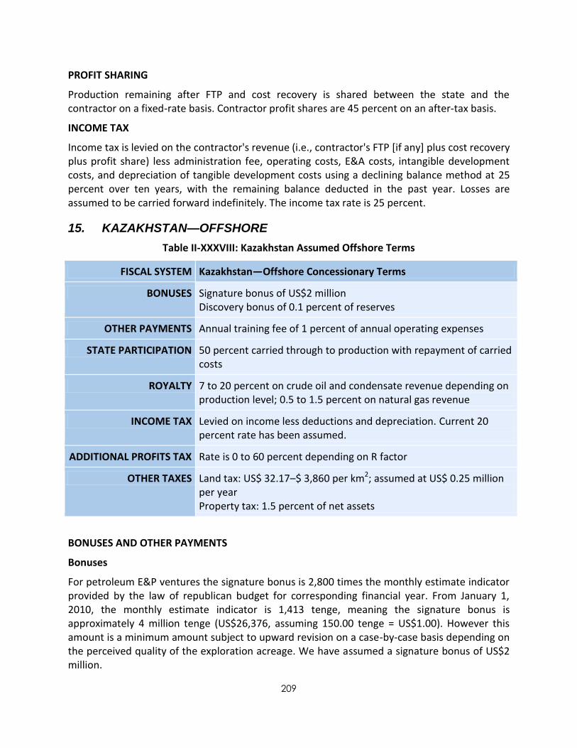
209

PROFIT SHARING

Production remaining after FTP and cost recovery is shared between the state and the contractor on a fixed-rate basis. Contractor profit shares are 45 percent on an after-tax basis.

INCOME TAX

Income tax is levied on the contractor's revenue (i.e., contractor's FTP [if any] plus cost recovery plus profit share) less administration fee, operating costs, E&A costs, intangible development costs, and depreciation of tangible development costs using a declining balance method at 25 percent over ten years, with the remaining balance deducted in the past year. Losses are assumed to be carried forward indefinitely. The income tax rate is 25 percent.

15. KAZAKHSTAN—OFFSHORE

Table II-XXXVIII: Kazakhstan Assumed Offshore Terms

FISCAL SYSTEM Kazakhstan—Offshore Concessionary Terms

BONUSES Signature bonus of US$2 million Discovery bonus of 0.1 percent of reserves

OTHER PAYMENTS Annual training fee of 1 percent of annual operating expenses

STATE PARTICIPATION 50 percent carried through to production with repayment of carried costs

ROYALTY 7 to 20 percent on crude oil and condensate revenue depending on production level; 0.5 to 1.5 percent on natural gas revenue

INCOME TAX Levied on income less deductions and depreciation. Current 20 percent rate has been assumed.

ADDITIONAL PROFITS TAX Rate is 0 to 60 percent depending on R factor

OTHER TAXES Land tax: US$ 32.17–$ 3,860 per km2; assumed at US$ 0.25 million per year Property tax: 1.5 percent of net assets


Bonuses

For petroleum E&P ventures the signature bonus is 2,800 times the monthly estimate indicator provided by the law of republican budget for corresponding financial year. From January 1, 2010, the monthly estimate indicator is 1,413 tenge, meaning the signature bonus is approximately 4 million tenge (US$26,376, assuming 150.00 tenge = US$1.00). However this amount is a minimum amount subject to upward revision on a case-by-case basis depending on the perceived quality of the exploration acreage. We have assumed a signature bonus of US$2 million.

210

A discovery bonus is payable at the rate of 0.1 percent of the value of approved recoverable reserves.

Training Fee

A training fee is calculated as a negotiated percentage of the overall annual operating budget expenditure. One percent of annual operating costs is indicative of past contracts and is assumed here.

Other payments including contributions for the use of water and forests (if applicable) and to an environment protection fund are required. Amounts payable into such funds are negotiable. A total of $0.6 million per year has been assumed for such payments.

STATE PARTICIPATION

The terms for state participation are determined on a contract-by-contract basis. In past joint ventures a local partner (in the form of a state-owned entity) has typically participated on a carried interest basis at a negotiable percentage, usually 50 percent. We assume a 50 percent state interest in the project which is carried from the start of the project through to the commencement of commercial production with no repayment of carried costs.

ROYALTY

A sliding scale Mineral Extraction Tax (MET), a royalty-type levy, is levied on the value of the production of crude oil, gas condensate, and natural gas. (2008 TC Art 336). The following royalty rates apply from January 1, 2009:

Table II-XXXIX: Kazakhstan Crude Oil Royalty Rate

Volume of annual crude oil or gas

condensate production

(thousand tons)

Equivalent daily

production (mbd)

Mineral Extraction Tax Rate (percent) commencing

January 1, 2009


January 1, 2013


January 1, 2014

Up to 250 inclusive 0–5 5 6 7 Up to 500 inclusive 5–10 7 8 9

Up to 1,000 inclusive 10–20 8 9 10 Up to 2,000 inclusive 20–40 9 10 11 Up to 3,000 inclusive 40–60 10 11 12 Up to 4,000 inclusive 60–80 11 12 13 Up to 5,000 inclusive 80–100 12 13 14 Up to 7,000 inclusive 100–140 13 14 15

Up to 10,000 inclusive 140–200 15 16 17 In excess of 10,000 > 200 18 19 20

211

Natural Gas

The MET rate for natural gas that is exported is 10 percent. For natural gas that is sold on Kazakhstan's domestic market, the MET rate is reduced to between 0.5 and 1.5 percent depending on annual production, as follows:

Table II-XL: Kazakhstan Royalty for Natural Gas Sold in Domestic Market

Volume of annual natural gas production

(billion cubic meters)

Daily volume of natural gas (MMcf per day)

Mineral Extraction Tax Rate (percent)

Up to 1 inclusive 0–100 0.5

Up to 2 inclusive 100–200 1.0

In excess of 2 > 200 1.5

EXPORT RENT TAX

Quantities of crude oil and gas condensate exported from the republic of Kazakhstan are subject to an annual tax (export rent tax). For this study sale in the domestic market has been assumed and domestic market price differentials have been applied.

INCOME TAX

Income tax is levied on taxable income (i.e., revenue less deductions and depreciation) in accordance with the provisions of the 2008 Tax Code. Bonuses are capitalized and depreciated at 25 percent. We have assumed straight-line depreciation over four years from the start of commercial production. Operating expenses, E&A costs, royalty, and other taxes except excess profits tax, contributions to decommissioning funds, and training fees are also expensed and deducted immediately.

We assume tangible development costs are capitalized and depreciated at 10 percent annually while all other development costs are capitalized and depreciated at 15 percent annually.

The income tax rates from January 1, 2011, can be summarized as follows:

Table II-XLI: Kazakhstan Income Tax Rate

Calendar Year Income Tax Rate (percent)

2011 20.0

2012 20.0

2013 17.5

2014 and thereafter 15.0

Note: We have applied the 20 percent rate applicable in 2011.

212


Known as excess profits tax (EPT) and levied on the difference between the annual net income and 25 percent of the annual deductions allowable for income tax. We define net income as taxable income for income tax less income tax payable. The rate of EPT is determined by an incremental sliding scale based on an R factor as follows:

Table II-XII: Kazakhstan Excess Profit Tax Rates

R Factor Excess Profits Tax Rate (percent)

< 1.25 0.0

1.25 < R < 1.30 10.0

1.30 < R < 1.40 20.0

1.40 < R < 1.50 30.0

1.50 < R < 1.60 40.0

1.60 < R < 1.70 50.0

R > 1.70 60.0

The R factor is the ratio of accumulated income to accumulated expenses. We define expenses as the sum of operating costs, capital expenditure, social and infrastructure payments, environmental monitoring fee, property tax, land tax, training fee, royalty, and income tax.

OTHER TAXES

Land Tax

Rates of land tax for land for industrial use located beyond populated localities range from 48.25 to 5,790 tenge per hectare (US$ 32.17 to US$ 3,860 per km2) depending on the perceived quality of the land.192 Annual land tax is assumed to be US$ 0.25 million per year.

Property Tax

Property tax is levied on net assets (assumed to be cumulative capital expenditure less cumulative depreciation). The rate of property tax is 1.5 percent.193

192 2008 Tax Code Art 383.1 193 2008 Tax Code Art 398.1

213

16. LIBYA—ONSHORE

Table II-XLIII: Libya Assumed Onshore Terms

FISCAL SYSTEM Libya—EPSA IV Onshore Terms

BONUSES Signature bonus of US$10 million Production bonuses of US$1, US$5, and US$3 million payable at production start-up, on 100 MMboe per day and for each 30 MMboe per day thereafter

OTHER PAYMENTS Annual Training Fee of US$200,000

STATE PARTICIPATION 50 percent participation carried to discovery without repayment of past costs 85 percent participating interest in operating costs

ROYALTY Paid by the state

COST RECOVERY From contractor share of gross production

PROFIT SHARING On a sliding scale linked to daily production (oil only) and Revenue/Cost Ratio Oil: 4–80.75 percent (A Factor * B Factor) Gas: 20–.85 percent

INCOME TAX Paid by the state


A negotiable signature bonus is payable. A bonus of US$10 million has been assumed. Production bonuses are payable with respect to each commercial discovery as follows:

Table II-XLIV: Libya Production Bonuses

PRODUCTION BONUSES

Cumulative Production Bonus (million US dollars)

Oil (million barrels) Gas (billion cubic feet)

Production start-up Production start-up 1.0

100 566 5.0

and for each 30 thereafter and for each 170 thereafter 3.0

Funding for a training program is required during the exploration and exploitation phases. An annual training fee of US$200,000 from project start-up has been assumed here.

Bonuses and training fees are nonrecoverable costs.

214

STATE PARTICIPATION

The Libyan National Oil Company takes a 50 percent working interest upon commercial discovery but does not reimburse its share of past E&A costs. The NOC pays an equal share (50 percent) of development costs and abandonment/decommissioning costs1. Operating expenses are shared between the NOC and the contractor in the same proportion as the percentage of production allocated to the NOC; 85 percent has been assumed here.194

ROYALTY

The contractor's royalty liability is discharged by the NOC from its share of revenue from the project.195

COST RECOVERY

Recoverable costs are expensed and recovered immediately from production remaining after the NOC's production allocation. Unrecovered costs may be carried forward indefinitely until fully recovered but not beyond the duration of the contract.

PROFIT SHARING

All production remaining after the NOC's allocation and cost recovery is shared between the NOC and the contractor on the basis of B and A Factors, which are biddable. The contractor's share is calculated as follows:

Contractor’s profit share = Excess Petroleum * (B Factor) * (A Factor)

B factor is calculated based on daily production rates; the following parameters have been assumed here:

Table II-XLV: Libya Profit Sharing (B Factor)

B FACTOR196

Average Daily Oil Production (mbd) B Factor

0–20 0.95

20–30 0.80

30–60 0.60

60–85 0.40

> 85 0.20

For gas production B factor is set at 1 (one).

"A" factor is applied to each calendar year on the basis of the ratio of the contractor's cumulative revenues to cumulative costs (R factor) for the preceding calendar year.

194

NOC production allocation is a bid variable. 195

2005 Onshore Model Contract Art 19.1, Exhibit F. 196

The assumptions used here are based on the example calculation in the Exhibit E of the 2005 Onshore Model Contract.

215

Table II-XLVI: Libya Profit Sharing (A Factor)

A FACTOR197

Ratio A Factor

< 1.5 0.85

1.5–3.0 0.75

3.0–4.0 0.40

> 4.0 0.20

INCOME TAX

The contractor's income tax liability is discharged by the NOC from its share of revenue from the project.

17. MALAYSIA—OFFSHORE

Table II-XLVII: Malaysia Assumed Terms

FISCAL SYSTEM Malaysia—PSA Offshore Terms

BONUSES None

OTHER PAYMENTS Annual training fee of US$100,000 during the exploration period is assumed Research CESS fee of 0.5 percent of contractor's cost oil/gas and profit oil/gas

STATE PARTICIPATION 40 percent carried through to discovery without repayment of carried costs

ROYALTY 10 percent of gross production

COST RECOVERY From 70–30 percent of gross production depending on the contractor's R/C ratio Excess cost recovery attributable to the contractor: 80–20 percent depending on the contractor's R/C ratio and cumulative production

PROFIT SHARING 80–10 percent of gross production after royalty and cost recovery depending on the contractor's R/C ratio and cumulative production

EXCESS PROFITS PAYMENTS 70 percent of profit oil/gas in excess of base price (only if contractor's R/C ratio exceeds 1.0)

INCOME TAX 38 percent of income less deductions and depreciation

197

Ibid.

216


There is no provision for payment of signature or discovery bonuses.

The contractor is required to provide for the training of Petronas, the NOC, personnel. The minimum amount required is negotiable and recorded in the contract, but normally specified as a number of man-months of training over the contract term. We have assumed a training fee of US$100,000 per annum during the exploration period based on indicative amounts from signed contracts. Training fee is a recoverable cost and assumed to be deductible for income tax purposes.

Research "cess" equal in value to 0.5 percent of the contractor's share of cost oil/gas and profit oil/gas is payable to Petronas. The research cess is a nonrecoverable cost but is deductible for income tax.

STATE PARTICIPATION

Petronas is entitled to a negotiable participating interest in a contract, subject to a minimum of 15 percent. Petronas’s interest is carried until the completion of three wildcat exploration wells without the repayment of carried costs. We have assumed a 40 percent interest carried through to commercial discovery without the repayment of carried costs.

ROYALTY

Royalty for both oil and gas is set at a maximum of 10 percent of gross production, which has been assumed here. Although the 10 percent rate is described as a maximum, no lower percentage has yet been applied.

COST RECOVERY

All recoverable costs are expensed and recovered immediately from a percentage of gross production determined by a sliding scale tied to the contractor's revenue to cost ratio (R/C ratio). Unrecovered costs may be carried forward indefinitely until fully recovered but not beyond the duration of the contract. Petroleum available for cost recovery but not used for such purpose (i.e., excess cost recovery) is shared between the state and contractor on a sliding scale as determined by the contractor's R/C Ratio and cumulative production. The following table contains the assumed cost recovery ceiling rates and excess cost recovery sharing rates:

217

Table II-XLVIII: Malaysia Cost Recovery Ceiling

COST RECOVERY

Contractor’s R/C Ratio


(percent of gross production)

Contractor's Share of Excess Cost Recovery (percent)

(i.e., Unused Cost Recovery)

Cum. Production ≤ Cum. THV198

Cum. Production > Cum. THV

0 < R/C ≤ 1.0 70 Not applicable Not applicable 1.0 < R/C ≤ 1.4 60 80 40 1.4 < R/C ≤ 2.0 50 70 40 2.0 < R/C ≤ 2.5 30 60 40 2.5 < R/C ≤ 3.0 30 50 40

R/C > 3.0 30 40 20

PROFIT SHARING

Production remaining after royalty and cost recovery is shared between the state and the contractor on a sliding scale determined by the contractor's R/C Ratio and cumulative production. The following has been assumed:

Table II-XLIX: Malaysia Profit Sharing

PROFIT SHARING

Contractor’s R/C Ratio Contractor's Profit Share (percent)

Cumulative Production ≤ Cumulative THV

Cumulative Production > Cumulative THV

0 < R/C ≤ 1.0 80 40

1.0 < R/C ≤ 1.4 70 30

1.4 < R/C ≤ 2.0 60 30 2.0 < R/C ≤ 2.5 50 30 2.5 < R/C ≤ 3.0 40 30

R/C > 3.0 30 10

EXCESS PROFITS PAYMENTS

When the price of oil or the price of natural gas exceeds a negotiated base price and the contractor's R/C Ratio exceeds 1.0, the contractor must pay to Petronas from its share of profit oil or profit gas 70 percent of the amount by which the value of the profit oil or profit gas exceeds the base price. We have assumed a base price of $41.63 per barrel and $3 per Mcf respectively.

198

The Cumulative THV (Threshold Volume) is the sum of all individual THV in the contract area. Each field's THV is the lower of 30 million barrels (0.75 trillion cubic feet for gas fields) of gross production or the size of its proved ultimate recovery as stipulated under the development plan for the field.

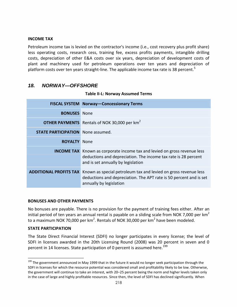
218

INCOME TAX

Petroleum income tax is levied on the contractor's income (i.e., cost recovery plus profit share) less operating costs, research cess, training fee, excess profits payments, intangible drilling costs, depreciation of other E&A costs over six years, depreciation of development costs of plant and machinery used for petroleum operations over ten years and depreciation of platform costs over ten years straight-line. The applicable income tax rate is 38 percent.5

18. NORWAY—OFFSHORE

Table II-L: Norway Assumed Terms

FISCAL SYSTEM Norway—Concessionary Terms

BONUSES None

OTHER PAYMENTS Rentals of NOK 30,000 per km2

STATE PARTICIPATION None assumed.

ROYALTY None

INCOME TAX Known as corporate income tax and levied on gross revenue less deductions and depreciation. The income tax rate is 28 percent and is set annually by legislation

ADDITIONAL PROFITS TAX Known as special petroleum tax and levied on gross revenue less deductions and depreciation. The APT rate is 50 percent and is set annually by legislation


No bonuses are payable. There is no provision for the payment of training fees either. After an initial period of ten years an annual rental is payable on a sliding scale from NOK 7,000 per km2 to a maximum NOK 70,000 per km2. Rentals of NOK 30,000 per km2 have been modeled.

STATE PARTICIPATION

The State Direct Financial Interest (SDFI) no longer participates in every license; the level of SDFI in licenses awarded in the 20th Licensing Round (2008) was 20 percent in seven and 0 percent in 14 licenses. State participation of 0 percent is assumed here.199

199

The government announced in May 1999 that in the future it would no longer seek participation through the SDFI in licenses for which the resource potential was considered small and profitability likely to be low. Otherwise, the government will continue to take an interest, with 20–25 percent being the norm and higher levels taken only in the case of large and highly profitable resources. Since then, the level of SDFI has declined significantly. When

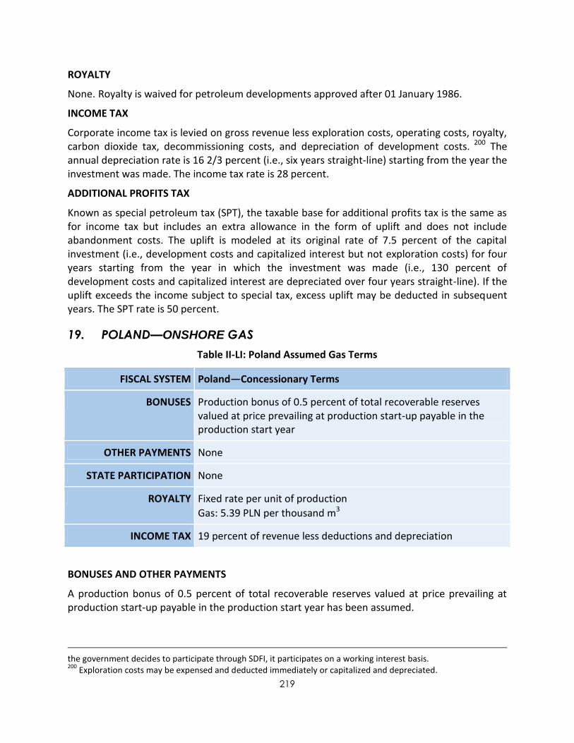
219

ROYALTY

None. Royalty is waived for petroleum developments approved after 01 January 1986.

INCOME TAX

Corporate income tax is levied on gross revenue less exploration costs, operating costs, royalty, carbon dioxide tax, decommissioning costs, and depreciation of development costs. 200 The annual depreciation rate is 16 2/3 percent (i.e., six years straight-line) starting from the year the investment was made. The income tax rate is 28 percent.


Known as special petroleum tax (SPT), the taxable base for additional profits tax is the same as for income tax but includes an extra allowance in the form of uplift and does not include abandonment costs. The uplift is modeled at its original rate of 7.5 percent of the capital investment (i.e., development costs and capitalized interest but not exploration costs) for four years starting from the year in which the investment was made (i.e., 130 percent of development costs and capitalized interest are depreciated over four years straight-line). If the uplift exceeds the income subject to special tax, excess uplift may be deducted in subsequent years. The SPT rate is 50 percent.

19. POLAND—ONSHORE GAS

Table II-LI: Poland Assumed Gas Terms

FISCAL SYSTEM Poland—Concessionary Terms

BONUSES Production bonus of 0.5 percent of total recoverable reserves valued at price prevailing at production start-up payable in the production start year

OTHER PAYMENTS None


ROYALTY Fixed rate per unit of production

Gas: 5.39 PLN per thousand m3



A production bonus of 0.5 percent of total recoverable reserves valued at price prevailing at production start-up payable in the production start year has been assumed.

the government decides to participate through SDFI, it participates on a working interest basis. 200

Exploration costs may be expensed and deducted immediately or capitalized and depreciated.

220

ROYALTY

Royalty is levied at a fixed rate per unit of production. The following table contains the currently applicable royalty rates established by the Regulation of the Council of Ministers of November 7, 2006, with effect from January 1, 2007:

Table II-LII: Poland Natural Gas Royalty

Royalty Rates (Effective 1 January 2007)

Hydrocarbon PLN USD

High-methane Natural Gas 5.39 per 1,000 m3 0.07437per Mcf Other Natural Gas 4.48 per 1,000 m3 0.06191 per Mcf

INCOME TAX

Levied on gross revenue less bonuses, royalty, operating costs, dry hole expenditure, and depreciation of other E&A and development costs over ten years on a straight-line basis. The applicable income tax rate at the time this report was written was 19 percent.

20. RUSSIA—ONSHORE

Table II-LIII: Russia Assumed Terms

FISCAL SYSTEM Russia—Post-2001 Concessionary Terms

BONUSES Negotiable signature bonus—US$41 million assumed

RENTAL Rental of US$1,511.63 per km2 assumed


VAT 18 percent on petroleum destined for Russian market and other countries in the CIS

EXPORT DUTY None. Assumed sale in domestic market

ROYALTY Known as Minerals Production Tax (MPT) and levied on physical production. Rate for crude oil equates to approximately 20 percent for oil prices greater than US$50 per barrel Rate for natural gas equates to approximately US$0.14 per Mcf


OTHER TAXES Property tax: 2 percent of cumulative capital expenditure less cumulative capital expenditure depreciation

Land pollution tax: 0.1% of operating expenses

Unified Social Tax: levied on ”salary fund”; 21 percent average rate assumed; salary fund assumed as 6 percent of operating expenses

221


Signature bonus payments vary in relation to the types of rights being awarded. They vary from the equivalent of US$3,000 to US$100 million. A bonus of US$41 million has been assumed.

There is no legislative provision for training fees, although in practice the licensee may be expected to make financial provision for training.

STATE PARTICIPATION

None.

EXPORT DUTY

Export duties have not been modeled. Sale in domestic market has been assumed and VAT applies instead. The net back price has been adjusted to reflect sales in domestic market.

ROYALTY

Known as Minerals Production Tax (MPT) (and also as "Unified Tax," "Mineral Extraction Tax," and "Useful Minerals Production Tax"), MPT is currently levied on the physical quantities of produced crude oil and natural gas. The MPT rate for crude oil is equal to a constant multiplied by two coefficients which reflect world oil prices and the percentage of reserves produced to date, respectively, as follows:

MPT = K * Cp * Cd

where

K = RUR 470 per ton201

Cp = (P—15) * (R / 261)

P = Average price of Urals Blend oil for the tax period in US$ per barrel R = Average value for the tax period of the RUR to USD exchange rate Cd is in the range 0.3 to 1.0 depending on the ratio (N/V) where: N = cumulative production V = total producible reserves in the approved development plan When the ratio (N/V) is less than 0.8 (i.e., when the reserves in the approved development plan are less than 80 percent depleted) Cd = 1.0 When the ratio (N/V) is equal to or greater than 0.8 but less than 1.0 Cd = 3.8—(3.5 * N / V) When the ratio (N/V) is equal to or greater than 1.0 Cd = 0.3

The MPT rate for crude oil equates to approximately 20 percent of production when the Urals blend price is greater than US$50 per barrel.

The MPT rate for natural gas is RUR 265 per 1,000 cubic meters.202

201

The RUR 470 per ton applies from January 2013. The applicable constants for 2011 and 2012 are RUR 419 and RUR 446 per ton, respectively. 202

The RUR 265/1,000 cubic meters applies from January 2013. The applicable rates for 2011 and 2012 are RUR 237 and RUR 251 per thousand cubic meters, respectively.

222

INCOME TAX

Known as profits tax and levied on gross revenue less operating costs, tariffs, VAT, Royalty, Road Fund Tax, Property Tax, Land and Pollution Taxes, Single Social Tax, and depreciation of exploration and development costs over 14 years on a straight-line basis (modeled as 7 percent per year). The income tax rate is 20 percent, with effect from January 1, 2009.

OTHER TAXES

Value Added Tax (VAT)

VAT is levied at the flat rate of 18 percent. Although recoverable, creditable, or refundable, investors have found VAT to be a significant burden owing to long delays or even failure to recover VAT refunds.

Property Tax (PRO)

Property tax is levied on cumulative capital expenditure less cumulative capital expenditure depreciation as for profits tax purposes. The rate of property tax is 2 percent.

Land and Pollution Tax (LNP)

Assumed to be equivalent to 0.1 percent of operating costs. Land tax is payable on a US$ per km2 basis and environmental payments are based on a US$ per unit of output basis. The rates differ regionally but are always negligible. We have adopted a simplified assumption that they total a small percentage of field operating costs each year to capture the indicative impact of these minor taxes.

Unified Social Tax (UST)

Unified Social Tax is an amalgamation of various mandatory payments. For the modeling purposes, we assume the total tax base of 6 percent of operating costs and an average rate of unified social tax of 21 percent.

223

21. UNITED KINGDOM—OFFSHORE

Table II-LIV: United Kingdom Assumed Offshore Terms

FISCAL SYSTEM United Kingdom—Concessionary Terms

BONUSES None

OTHER PAYMENTS Exploration rental: US$3,182 per year.

Production rental: Phase I—US$238.66 per km2; Phase II—US$477.33 per km2


ROYALTY None

COST RECOVERY Not applicable

PROFIT SHARING Not applicable

INCOME TAX Corporation tax is levied at 30 percent on gross revenue less deductions and depreciation.

ADDITIONAL PROFITS TAX Supplementary charge is levied at 32 percent on the same taxable base as for income tax (except for financing costs) less a field allowance where applicable.


There is no provision for the payment of bonuses or training fees.

The amount of rental payable is prescribed for each round. Rental rates are subject to biennial review in line with movements in the Index of the Price of Crude Oil acquired by Refineries. Adjustment may only be made if the movement in such index exceeds 5 percent lower or higher in the relevant period.

For an exploration license a one-time payment of £2,000 is required. The following table contains rental payments for production licenses that applied in the latest licensing rounds.

Table II-LV: United Kingdom Rentals

Round Period (years) Rental (£ per km²)

20–25 1–4 150 20–25 5 and thereafter £300 increased by £900 per km² each year

until £7,500 per km² is reached

224

STATE PARTICIPATION

None.

ROYALTY

None.

INCOME TAX

Known as corporation tax and levied on gross revenue less operating costs, exploration costs, and development costs. The applicable tax rate in the United Kingdom is 30 percent. The general corporate tax rate has been reduced from 30 to 26 percent; however the reduced rate does not apply to upstream petroleum activities.


The supplementary petroleum tax (SC), levied at 32 percent, although not strictly tax on additional profits, is levied on the same basis as for corporation tax except that financing charges are not deductible. Certain fields given development approval on or after 22 April 2009 benefit from a field allowance that is deductible from the taxable income subject to SC. The field allowance is a fixed amount per company and is subject to an annual limit. It applies to selected types of fields; this model considers only the field allowance given to small fields, which is £75 million for fields with recoverable reserves <2.75 million tons of oil equivalent (US$112.5 million for reserves < 20.075 MMboe) reducing on a straight-line basis to £0 (zero) for fields with recoverable reserves > 3.5 million tons of oil equivalent (US$0 [zero] for reserves > 25.55 MMboe). The maximum annual allowance is £15 million (US$22.5 million).

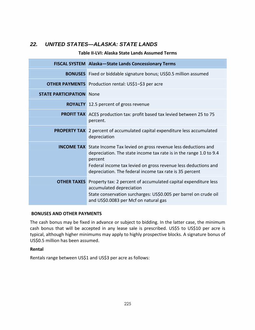
225

22. UNITED STATES—ALASKA: STATE LANDS

Table II-LVI: Alaska State Lands Assumed Terms

FISCAL SYSTEM Alaska—State Lands Concessionary Terms

BONUSES Fixed or biddable signature bonus; US$0.5 million assumed

OTHER PAYMENTS Production rental: US$1–$3 per acre


ROYALTY 12.5 percent of gross revenue

PROFIT TAX ACES production tax: profit based tax levied between 25 to 75 percent.

PROPERTY TAX 2 percent of accumulated capital expenditure less accumulated depreciation

INCOME TAX State Income Tax levied on gross revenue less deductions and depreciation. The state income tax rate is in the range 1.0 to 9.4 percent

Federal income tax levied on gross revenue less deductions and depreciation. The federal income tax rate is 35 percent

OTHER TAXES Property tax: 2 percent of accumulated capital expenditure less accumulated depreciation

State conservation surcharges: US$0.005 per barrel on crude oil and US$0.0083 per Mcf on natural gas


The cash bonus may be fixed in advance or subject to bidding. In the latter case, the minimum cash bonus that will be accepted in any lease sale is prescribed. US$5 to US$10 per acre is typical, although higher minimums may apply to highly prospective blocks. A signature bonus of US$0.5 million has been assumed.

Rental

Rentals range between US$1 and US$3 per acre as follows:

226

Table II-LVII: Alaska Rentals

Year Rental Rate (US$ per acre)

Year 1 1.00 Year 2 1.50 Year 3 2.00 Year 4 2.50

Year 5 onward 3.00

Source: IHS CERA

STATE PARTICIPATION

There is no provision for state participation.

ROYALTY

All leaseholders in Alaska are liable to pay royalty on their production. For most current producers the royalty is payable to the state, as the owner of the land. Royalty is levied on gross wellhead revenue, referred to as the “field price.” If the oil, gas or associated substance is sold off of the leased premises, the field price is calculated as the price realized less the actual and reasonable transportation costs. We have assumed a 12.5 percent royalty rate, the applicable rate from recent lease sales.

PROPERTY TAX

The state imposes the oil and gas property tax under the Oil and Gas Exploration, Production and Pipeline Transportation Property Taxes Act, Alaska Statutes Title 43 Chapter 56 (AS 43.56). The tax is assessed at the rate of 2 percent of the value of taxable exploration, production, and pipeline transportation property located within the state of Alaska. For tax purposes, exploration property is valued at the estimated price the property would be sold at in the open market under the then prevailing market conditions between a willing seller and a willing buyer; production property is valued on the basis of replacement costs of similar new property less depreciation based on the economic life of the proved reserves; and pipeline transportation property is valued based on its economic value relative to the reserves feeding into the pipeline.

STATE CONSERVATION SURCHARGES ON OIL

The state collects a conservation surcharge of US$0.01 per barrel of oil produced less royalty to fund the Release Response Account of the Oil and Hazardous Substance Release Prevention and Response Fund.203 The state also collects an additional conservation surcharge of US$0.04 per barrel of oil produced less royalty to fund Release Prevention Account of the Oil and Hazardous Substance Release Prevention and Response Fund. A total conservation tax of US$0.05 per barrel (or US$0.0083 per Mcf on an equivalence basis assuming 6,000 cubic feet of natural gas is equivalent to one barrel of oil) of gross production less royalty has been assumed.

203

The conservation Surcharge on Oil may be suspended if the balance of the Response Account of the Oil and Hazardous Substance Release Prevention and Response Fund exceeds US$50 million.

227

INCOME TAX

All leaseholders are liable to pay both federal and state income taxes. The latter include Alaska Corporate Income Tax and Alaska's Clear and Equitable State production tax (ACES).

Alaska Corporate Income Tax

The state of Alaska imposes a state income tax under the Alaska Net Income Tax Act, Alaska Statutes Title 43 Chapter 20 (AS 43.20) on income derived from sources in Alaska.

Alaska has adopted the U.S. Code for establishing deductions and depreciation in establishing taxable income, with the following exceptions:

taxes based on or measured by net income that are deducted in the determination of the federal taxable income are added back (except for ACES and conservation oil surcharges)

intangible drilling and development costs that are deducted as expenses in the determination of the federal taxable income are capitalized and depreciated

percentage depletion is recomputed and deducted on cost depletion basis

Oil and gas producers are assessed on the part of their worldwide income apportioned to Alaska. The apportionment factor is calculated as an average of

sales factor: producer's sales in Alaska (including pipeline tariffs received) divided by producer's sales worldwide (including pipeline tariffs received)204

property factor: average value of real and tangible property owned or rented by the producer plus intangible costs related to producing oil and gas wells in Alaska divided by the average value of real and tangible property owned or rented by the producer plus intangible costs related to producing oil and gas wells worldwide

extraction factor: oil and gas production volume in Alaska divided by the oil and gas production volume worldwide

The following credits may be used to reduce Alaska Corporate Income Tax liability:

Education Credit

Gas Exploration and Development Tax Credit

Exploration Incentive Credit

For simplification it is assumed state income tax is levied on gross revenue less royalty, other state taxes, operating costs, and depreciation of all capital costs on a unit of production basis. Alaska Corporate Income Tax rate is based on an incremental sliding scale as follows:205

204

Sales factor is calculated only for companies engaged in both production and pipeline transportation of oil and gas. 205

AS 43.20.011(e).

228

Table II-LVIII: Alaska Corporate Income Tax Rates

Increment of Taxable Income (U.S. dollars)

State Income Tax Rate (percent)

< 10,000 1.00

10,000–20,000 2.00

20,000–30,000 3.00

30,000–40,000 4.00

40,000–50,000 5.00

50,000–60,000 6.00

60,000–70,000 7.00

70,000–80,000 8.00

80,000–90,000 9.00

> 90,000 9.40

Alaska's Clear and Equitable State Production Tax (ACES)

The state of Alaska imposes a production tax under the Oil and Gas Production Taxes and Oil Surcharge, Alaska Statutes Title 43 Chapter 55 (AS 43.55) on oil and gas produced in Alaska. Currently applicable production tax, ACES, replaced Petroleum Profits Tax (PPT) in November 2007. The application of ACES was made retroactive to July 1, 2007.

ACES rate consists of two elements:

1. Base rate of 25 percent; and

2. Additional progressive component calculated if the "production tax value" (i.e., taxable net cash flow as described below) per barrel of taxable petroleum production exceeds US$30, as follows:

a. 0.4 percent for each US$1 of the production tax value per barrel if the production tax value is in the range of US$30–$92.50 per barrel; or

b. 25 percent + 0.1 percent for each US$1 of the production tax value per barrel if the production tax value is above US$92.50 per barrel.

The rate under (b) cannot exceed 50 percent. In essence, this means the maximum ACES tax rate is 75 percent of the production tax value in times of extremely high oil prices. These provisions apply to both oil and gas production, with gas converted to barrels of oil equivalent using energy equivalence basis.

Producer's "lease expenditure" (i.e., operating and capital costs) are expensed and deducted from the value of taxable petroleum to arrive to the "production tax value" (net cash flow)

229

which forms the basis of the ACES liability calculation. (AS 43.55.160)

ACES tax liability can be summarized as follows:

ACES tax liability = [(Value—Costs) * ACES Tax Rate]—Credits

where:

Value = Production multiplied by price

Costs = Operating costs plus capital expenditure (excluding bonuses)

ACES Tax Rate = 25 percent plus 0.4 percent for every US$1 per barrel that this "net income" exceeds US$30 per barrel (reduced to 0.1 percent for every US$1 per barrel above US$92.50 per barrel) subject to a maximum rate of 75 percent

Credits = (20 percent capital expenditure spread over two years) plus base allowance (see above)

Federal Income Tax

All leaseholders are liable to pay federal income tax under the Internal Revenue Code, U.S. Code Title 26 (26 U.S.C.). Federal income tax is levied on gross revenues less royalty, Alaskan income tax, ACES, state conservation charges, environmental tax, property tax, operating costs, intangible costs, depreciation of tangible costs and depletion. Leasehold acquisition costs as well as geological and geophysical (G&G) capital are eligible under cost depletion. For standard depreciation, exploration dry hole costs as well as intangible development capital are expensed and deducted immediately. Other exploration capital and tangible development capital is depreciated on a declining balance basis over seven years,206 and depreciation of signature bonus and G&G expenses is on a unit of production basis.207 Losses may be carried forward for a maximum of 20 years. The current maximum federal corporate income tax rate is 35 percent.

Table II-LIX: U.S. Federal Corporate Income Tax Rates

Increment of Taxable Income (U.S. dollars) Tax Rate (percent)

0–50,000 15.0

50,000–75,000 15.0

75,000–10,000,000 34.0

Exceeds 10,000,000 35.0

Note: We have assumed the maximum rate of 35 percent.

206 The life of assets varies from 3 to 25 years. Both 150 and 200 percent declining balance may be used, depending on the exact life of the asset. We have used 150 percent and a ten-year life as an average. 207

Leasehold acquisition costs (i.e., signature bonus) as well as G&G capital are eligible under cost depletion, which effectively is a depreciation using the unit of production method.

230

23. UNITED STATES—LOUISIANA: STATE LANDS

Table II-LX: Louisiana State Lands Assumed Terms

FISCAL SYSTEM U.S.A.—Louisiana: Concessionary Terms on State Lands

BONUSES Signature bonus of US$641 per acre

OTHER PAYMENTS Rental of US$320 per acre



FEDERAL INCOME TAX 35 percent of income less deductions and depreciation

STATE INCOME TAX 8 percent of income less allowable deductions and depreciation

SEVERANCE TAX Oil: 12.5 percent of gross revenue (at wellhead) Gas: US$0.331 percent per Mcf

PROPERTY TAX 1 percent


Biddable signature bonuses vary widely. A US$641 per acre bonus has been modeled based on results of recent lease sales.

RENTAL

Half of the cash payment made for acquisition of acreage is considered to be first year rental. The rental amount payable in subsequent years is equivalent to one half of the cash payment. Rentals offered in recent sales have been one half the amount offered as signature bonus. A rental of US$320 per acre has been assumed for this study.

ROYALTY

The statutory prescribed minimum royalty is 12.5 percent. However, the State Mineral Board has not accepted a 12.5 percent royalty in a long time. Royalties offered in recent lease sales have varied between 21 and 25 percent. A 23.4 percent royalty rate, representing the average rate from recent sales, has been assumed.

INCOME TAX

All leaseholders are liable to pay both federal and state income taxes. Federal income tax is payable at a corporate level on all income generated in the United States. The State of Louisiana levies a corporate income tax on income deriving from sources in Louisiana.

231

Federal Income Tax

Federal income tax is levied on gross revenue less royalty, operating costs, abortive exploration (i.e., dry hole) costs, intangible development costs, depreciation of other exploration costs (apart from G&G costs and dry hole costs), and tangible development expenditure on a declining balance basis over seven years, and depreciation of signature bonus and G&G expenses on a unit of production basis. Losses may be carried forward for a maximum of 20 years.

Income tax is levied on increments of taxable income at different rates depending on the level of taxable income. The current maximum federal corporate income tax rate is 35 percent. See Table II-LXII for applicable corporate income tax rates.

State Income Tax Corporations pay tax on net income computed at the following rates:

Table II-LXI: Louisiana Corporate Income Tax Rates

Increment of Taxable Income (U.S. dollars) Tax Rate (percent)

0–25,000 4.0

25,000–50,000 5.0

50,000–$100,000 6.0

100,000–200,000 7.0

Exceeds 200,000 8.0

Louisiana tax law allows for federal income tax deduction. We have assumed the maximum rate of 8 percent.

SEVERANCE TAX

The natural gas production tax, which is otherwise referred to as severance tax or occupation tax, is a tax on the production of crude oil and natural gas in the state of Louisiana.

The tax rate is US$0.331 per Mcf of gas produced and 12.5 percent of the market value of crude oil which is produced and saved. The market value of oil and gas is its value at the wellhead.

PROPERTY TAX

Louisiana parishes levy local property taxes on equipment for production of oil and gas. The rates vary by parish. The actual tax payable is computed by multiplying the assessed value times “the millage.” The assessed value for residential and commercial land is 10 percent of the market value. The millage is based on an archaic monetary unit called a mil. One mil equals one thousandths of a dollar. The average millage among Louisiana’s 64 parishes is 101 mils. For this study, we have assumed a rate of 10 percent of the “assessed value” of equipment, i.e., a 1 percent effective tax rate.

232

24. UNITED STATES—TEXAS: STATE LANDS

Table II-LXII: Texas State Lands Assumed Terms

FISCAL SYSTEM U.S.A.—Texas: State Lands


OTHER PAYMENTS Rental of US$5–$25.0 per acre


ROYALTY 25 percent of gross revenue


STATE INCOME TAX None

SEVERANCE TAX Oil: 4.6 percent of gross revenue (at wellhead) Gas: 7.5 percent of gross proceeds (minus transportation and processing cost)

PROPERTY TAX 2 percent of gross revenue


Biddable signature bonuses vary widely. A US$620 per acre bonus has been modeled based on results of recent lease sales.

RENTAL

Annual rentals are due and payable in advance on the first day of each lease year prior to the discovery of oil or gas. The following table contains the amount of rentals payable under recent lease sales.

Table II-LXIII: Texas Rental Rates

Year Rental

2–3 US$5 per acre 4–5 US$25 per acre

ROYALTY

The standard royalty rate prescribed in recent lease sales in Texas is 25 percent. The rate can be reduced to

20 percent if production, in paying quantities, is established, brought onstream, and sales thereof are commenced within the initial eighteen months of the primary term of the lease.

233

22.5 percent if production, in paying quantities, is established, brought onstream, and sales thereof are commenced between the 19th and 24th month of the primary term of the lease.

If the initial well drilled is a dry hole, the lessee may receive the lower royalty rate as follows:

20 percent if a second well is commenced and production, in paying quantities, can be established, brought onstream, and sales thereof are commenced by the end of the 21st month, as provided for in the lease.

22.5 percent if a second well is commenced and production, in paying quantities, can be established, brought onstream, and sales thereof are commenced by the end of the 27th month, as provided for in the lease.

For this study we have used the standard 25 percent royalty rate.

INCOME TAX

All leaseholders are liable to pay federal income tax under the Internal Revenue Code, U.S. Code Title 26 (26 U.S.C.). Federal income tax is payable at a corporate level on all income generated in the United States. The State of Texas does not levy income tax.


Income tax is levied on increments of taxable income at different rates depending on the level of taxable income. The current maximum federal corporate income tax rate is 35 percent. See Table II-LXII for applicable corporate income tax rates.

SEVERANCE TAX

The natural gas production tax, which is otherwise referred to as severance tax or occupation tax, is a tax on the production of crude oil and natural gas in the state of Texas.208

The tax rate is 7.5 percent of the market value of the gas and 4.6 percent of the market value of crude oil which is produced and saved. The market value of oil and gas is its value at the wellhead. Often there is no market for the gas at the wellhead owing to either the location of the well or the condition of the gas. The costs incurred in getting the gas to the market are deductions from the gross cash receipts and are referred to as marketing costs.

Severance tax relief granted for marginal wells does not apply in this case.209

208

Chapter 201 of the Texas Tax Code. 209

The tax code provides three levels of tax credits on gas production from qualified low-producing gas wells for any given month, depending on the Comptroller's average taxable oil and gas prices, adjusted to 2005 dollars, based on applicable price indices of the previous three months. An operator of a qualifying low-producing gas well would be entitled to

(1) a 25 percent tax credit if the average taxable gas price were more than $3.00 per Mcf but not more than $3.50 per Mcf

(2) a 50 percent tax credit if the price were more than $2.50 per Mcf but not more than $3.00 per Mcf

234

PROPERTY TAX

Texas counties do levy local property taxes on the estimated present value of minerals in the ground as well as structures and equipment used to produce oil and natural gas. The rates vary by county and usually range between 1.5 and 2.5 percent on gross revenues. A rate of 2 percent has been assumed.

FIELD CLEAN-UP REGULATORY FEE

The tax rate of one fifteenth (1/15) of one cent (US$0.000667) for each Mcf of gas produced was imposed effective September 1, 2001. The tax rate was increased in 2001 from the previously applicable rate of one thirtieth (1/30) of one cent (or US$0.000333) for each Mcf) of the gas produced. Up until August 31, 2003, the oil field clean-up tax did not apply to high-cost gas. The exemption was removed effective September 1, 2003.

25. UNITED STATES—OUTER CONTINENTAL SHELF: DEEPWATER GULF OF MEXICO

Table II-LXIV: U.S. GOM Assumed Deepwater Terms

FISCAL SYSTEM U.S.A.—Gulf of Mexico Concessionary Terms Deepwater Greater than 200 m (For lease sales held after 2008)

BONUSES Signature bonus of US$20–$100 million

OTHER PAYMENTS Rental of US$11–$44 per acre





A minimum U.S. dollar amount per acre is specified in the notice of sale. Biddable signature bonuses vary widely. Amounts of US$20 million to US$100 million have been modeled for the deepwater fields.

Annual rentals are due and payable in advance on the first day of each lease year prior to the discovery of oil or gas. The following table contains the amount of rentals payable under recent lease sales in deepwater Gulf of Mexico.

(3) a 100 percent tax credit if the price were $2.50 per Mcf or less

The tax code defines a qualifying low-producing gas well as a well that averages, over a three-month period, 90 Mcf per day or less. The tax credit is limited only to wells currently paying full tax rates (it excludes those wells operating under existing tax incentive programs). For the past five years the gas price has been above the qualifying threshold for the marginal gas well tax credit; therefore no wells qualified for this incentive.

235

Table II-LXV: U.S. GOM Deepwater Rentals

Water Depth (meters) Year Rental (U.S. dollars per acre)

200–400 1–5 11 6 22 7 33

8+ 44

400 + 1–5 11

Source: IHS CERA

ROYALTY

Since 2008 the applicable royalty rate for new leases has been 18.75 percent. The standard royalty rate has been modeled for this study. Where applicable, deep gas and ultradeep gas royalty relief has been applied. Since the threshold price for such relief is capped at US$4.16 per MMBtu, the relief was applied only in the low price scenario of US$4 per Mcf for this study.

INCOME TAX

All leaseholders are liable to pay federal income tax under the Internal Revenue Code, U.S. Code Title 26 (26 U.S.C.). Federal income tax is payable at a corporate level on all income generated in the United States. Petroleum activities in the continental shelf areas are subject to federal taxation only. State taxation laws do not apply to the outer continental shelf.

Federal income tax is levied on gross revenue less royalty, operating costs, abortive exploration (i.e., dry hole) costs, intangible development costs, depreciation of other exploration costs (apart from G&G costs and dry hole costs) and tangible development expenditure on a declining balance basis over seven years, and depreciation of signature bonus and G&G expenses on a unit of production basis. Losses may be carried forward for a maximum of 20 years.

Income tax is levied on increments of taxable income at different rates depending on the level of taxable income. The current maximum federal corporate income tax rate is 35 percent. See Table II-LXII for applicable corporate income tax rates. We have assumed the maximum rate of 35 percent.

236

26. UNITED STATES—OUTER CONTINENTAL SHELF—GULF OF MEXICO SHELF

Table II-LXVI: U.S. GOM Assumed Shelf Terms

FISCAL SYSTEM U.S.A.—Gulf of Mexico Concessionary Terms Offshore less than 200 m Water Depth (For lease sales held after 2008)

BONUSES Signature bonus of US$250,000

OTHER PAYMENTS Rental of US$7–$28 per acre





A minimum U.S. dollar amount per acre is specified in the notice of sale (US$25 per acre in recent notices). Biddable signature bonuses vary widely. A US$250,000 bonus has been modeled for shelf fields.

RENTAL

Annual rentals are due and payable in advance on the first day of each lease year prior to the discovery of oil or gas. The following table contains the amount of rentals payable under recent lease sales in less than 200 meter water depth in the Gulf of Mexico.

Table II-LXVII: U.S. GOM Rental for Water Depth up to 200m

Water Depth (meters) Year Rental (U.S. dollars per acre)

< 200 1–5 7 6 14 7 21

8+ 28

ROYALTY

Since 2008 the applicable royalty rate for new leases has been 18.75 percent. Deep Gas and Ultra Deep Gas Royalty Relief has been applied for qualifying fields. Since the threshold price for such relief is capped at US$4.16 per MMBtu, the relief was applied only in the low price scenario of US$4 per Mcf for this study.

INCOME TAX

All leaseholders are liable to pay federal income tax under the Internal Revenue Code, U.S. Code Title 26 (26 U.S.C.). Federal income tax is payable at a corporate level on all income generated in the United States. Petroleum activities in the continental shelf areas are subject to federal

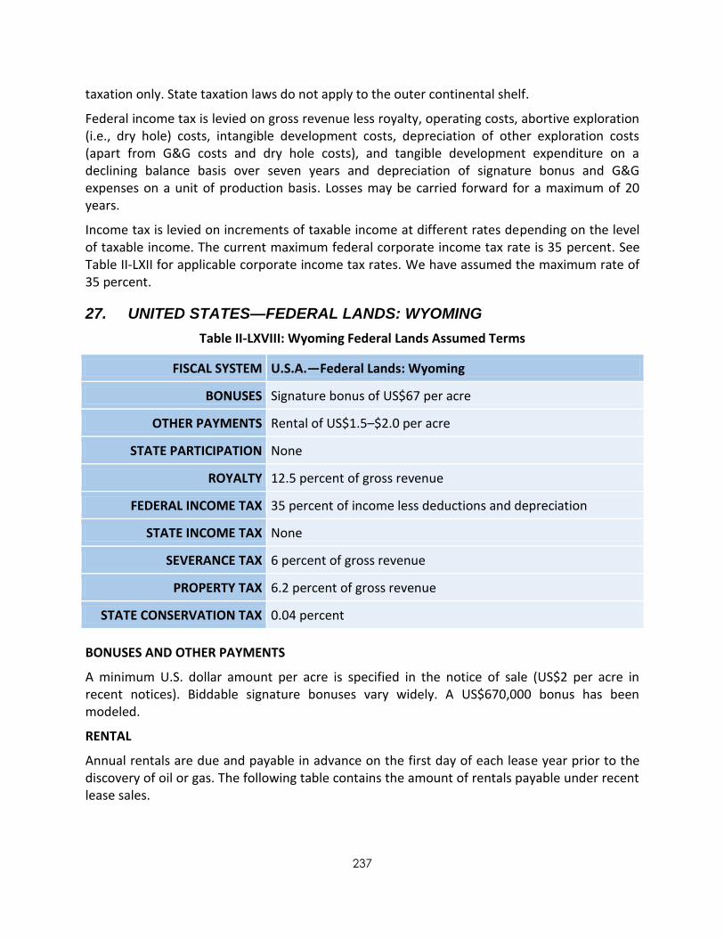
237

taxation only. State taxation laws do not apply to the outer continental shelf.

Federal income tax is levied on gross revenue less royalty, operating costs, abortive exploration (i.e., dry hole) costs, intangible development costs, depreciation of other exploration costs (apart from G&G costs and dry hole costs), and tangible development expenditure on a declining balance basis over seven years and depreciation of signature bonus and G&G expenses on a unit of production basis. Losses may be carried forward for a maximum of 20 years.


27. UNITED STATES—FEDERAL LANDS: WYOMING

Table II-LXVIII: Wyoming Federal Lands Assumed Terms

FISCAL SYSTEM U.S.A.—Federal Lands: Wyoming


OTHER PAYMENTS Rental of US$1.5–$2.0 per acre




STATE INCOME TAX None

SEVERANCE TAX 6 percent of gross revenue

PROPERTY TAX 6.2 percent of gross revenue

STATE CONSERVATION TAX 0.04 percent


A minimum U.S. dollar amount per acre is specified in the notice of sale (US$2 per acre in recent notices). Biddable signature bonuses vary widely. A US$670,000 bonus has been modeled.

RENTAL

Annual rentals are due and payable in advance on the first day of each lease year prior to the discovery of oil or gas. The following table contains the amount of rentals payable under recent lease sales.

238

Table II-LXIX: Wyoming Federal Rentals

Year Rental (U.S. dollars per acre)

1–5 1.5 6–10210 2

ROYALTY

The standard royalty rate on federal lands in Wyoming is 12.5 percent. Lower rates apply for marginal wells; however, the analysis of such terms is not within the scope of this study.211

INCOME TAX

All leaseholders are liable to pay federal income tax under the Internal Revenue Code, U.S. Code Title 26 (26 U.S.C.). Federal income tax is payable at a corporate level on all income generated in the United States. Petroleum activities onshore are usually subject to state income tax. The State of Wyoming does not levy income tax.



SEVERANCE TAX

An ad valorem tax of 6 percent is levied by the State of Wyoming. The tax is levied on the same basis as royalty, i.e., gross revenue minus transportation and gas processing cost.

PROPERTY TAX

An ad valorem tax is levied by counties on taxable value of previous year’s production. The tax ranges from 6 to 7.3 percent. We have assumed 6.2 percent rate, which is the statewide mineral tax district average.

OIL AND GAS CONSERVATION TAX

The State of Wyoming levies an oil and gas conservation tax at the rate of 0.04 percent of gross proceeds from oil and gas production.

210

The $2 per acre rental is for the remainder of the first term of the lease or until production starts, whichever occurs earlier. 211 The wells in the respective fields modeled do not qualify as marginal wells.

239

28. VENEZUELA—NON-ASSOCIATED GAS TERMS

Table II-LXX: Venezuela Assumed Non-associated Gas Terms

FISCAL SYSTEM Venezuela Non-associated Gas Concessionary Terms


OTHER PAYMENTS Social Fund: greater of 1 percent of gross production or US$1 million National Capital Participation: 1 percent of total investment Rental: US$1,512 per km2

STATE PARTICIPATION 35 percent carried through to discovery with repayment of carried costs without interest

ROYALTY 25 percent of gross revenue reduced by up to 15 percent of gross revenue in transportation costs

EXTRACTION TAX Not applicable

INCOME TAX 34 percent of gross revenue less deductions and depreciation

ANNUAL SPECIAL ADVANTAGE Not applicable

WINDFALL TAX ON OIL EXPORTS Not applicable


Signature bonuses are biddable. We have assumed a signature bonus of US$20 million based on the average amount of signature bonuses paid in the 2005-2006 Gulf of Venezuela license round by private oil companies.

Social Fund: annual contribution of the greater of 1 percent of total gas production or US$1 million.212

National Capital Participation: 1 percent of total investment under the license (i.e., capital expenditure but not bonuses).213 National capital participation in natural gas projects is payable throughout the contract duration, in four installments, as follows:

o 20 percent of the contribution at the time of the grant of the license—assumed to be payable in the project start year

212

Resolution 011 of February 2, 2006 (2006 RL) Art. 33. 213

Guidelines for Participation of National Capital in Natural Gas Projects, November 2002 (2002 NCPG) Art V.4.8.

240

o 20 percent of the contribution upon finalization of the minimum exploratory program—assumed to be payable upon discovery

o 30 percent of the contribution upon declaration of commercial discovery—assumed to be payable upon discovery;

o 30 percent of the contribution at the end of the basic engineering—assumed to be payable upon production start-up.

STATE PARTICIPATION

State participation at 35 percent carried to commercial discovery with repayment of carried costs (excluding bonuses) without interest is assumed here.

ROYALTY

Royalty is assumed to be levied on the gross revenue from the nonassociated gas project after deducting the lesser of (a) transportation costs (assumed to be represented by variable operating expenses) or (b) 15 percent of gross revenue. The royalty is modeled at the rate of 25 percent (general royalty of 20 percent plus special remuneration of 5 percent 3).

EXTRACTION TAX

Not applicable to nonassociated gas licenses.

INCOME TAX

Levied at 34 percent on taxable income, i.e., gross revenue less operating costs, royalty, signature bonus, social fund, national capital participation, dry hole expenditure, and depreciation of all other capital expenditure on the unit of production basis starting from the commencement of production.

ANNUAL SPECIAL ADVANTAGES


WINDFALL TAX ON OIL EXPORT


241

29. VENEZUELA—HEAVY OIL TERMS

Table II-LXXI: Venezuela Assumed Heavy Oil Terms

FISCAL SYSTEM Venezuela—Heavy Oil Joint Ventures


OTHER PAYMENTS Indigenous Development Programs: 1 percent of previous year's pretax profits

STATE PARTICIPATION 60 percent carried through to discovery with repayment of carried costs without interest

ROYALTY 33.33 percent of gross production

COST RECOVERY Not applicable

PROFIT SHARING Not applicable

EXTRACTION TAX 33.33 percent of gross production. Royalty and Annual Special Advantage are creditable

INCOME TAX 50 percent of gross revenue less deductions and depreciation

ANNUAL SPECIAL ADVANTAGE Difference between 50 percent of gross revenue and sum of all payments to the state

WINDFALL TAX ON OIL EXPORTS Sale in domestic market is assumed


A signature bonus of US$646 million has been assumed. The bonus payment is indicative of signature bonuses reported for awards made in 2010.

The contractor is required to invest annually 1 percent of its annual profits before taxes for the prior calendar year in indigenous development programs.

STATE PARTICIPATION

State participation at 60 percent carried to commercial discovery with repayment of carried costs (excluding bonuses) without interest is assumed.214

ROYALTY

Royalty is levied on volumes of oil and associated gas at a rate of 33.33 percent (general royalty of 30 percent plus additional royalty of 3.33 percent payable as a special advantage to the

214

State participation for extra heavy oil projects in Venezuela has varied between 60 and 80 percent. Over two thirds of the contracts awarded have provided for 60 percent state participation, which has been assumed here.

242

state).

EXTRACTION TAX

An amount equal to one third (i.e., 33.33 percent) of the value of all liquid hydrocarbons extracted is payable to the state. Royalty (including any additional royalty payable as a special advantage) for the current period and the amount of annual special advantage for the previous year (see below) can be credited against the extraction tax payable.

INCOME TAX

Levied at 50 percent on taxable income, i.e., gross revenue less operating costs, indigenous projects investments, royalty, extraction tax, dry hole expenditure, and depreciation of all other capital on the unit of production basis start from the commencement of production.

ANNUAL SPECIAL ADVANTAGES

Starting from April 20, 2007, an amount equal to the difference between (i) 50 percent of gross revenue and (ii) the sum of all payments made by the joint venture to the state (including royalty, additional royalty, income tax, any other tax or levy calculated based on revenues (whether net or gross), including indigenous project investments) is payable to the state annually as a special advantage. The amount of payment shall be equal to zero when (ii) is equal to or greater than (i).

WINDFALL TAX ON OIL EXPORT

A "windfall tax" is levied at a rate of 50 percent on oil revenues (from the export of liquid hydrocarbons and their products) between a Brent oil price of US$70 per barrel and US$100 per barrel and at a rate of 60 percent of revenues above a Brent oil price of US$100 per barrel. The tax is deductible for income tax purposes. The tax, which has been recently amended to increase the rate as well as introduce various price thresholds, provides exemptions for projects for the development of new reservoirs and those ongoing projects aimed at increasing production as long as they have not recovered their investments.215 This tax has not been modeled here.

215

Prior to the 2011 amendment of the windfall profits tax the joint ventures engaged in production of heavy oil were not subject to the windfall profits tax since the Hydrocarbon Law reserved the commercialization of natural hydrocarbons to 100 percent state-owned companies. Under the new law, discretionary exemptions may also be granted to various investment agreements.

243

APPENDIX III—RESULTS OF ECONOMIC ANALYSIS

Table III-I: Individual Project Indicators

Fiscal System No. Field Type Government Take PI IRR

Low Case

Base Case

High Case

Low Case

Base Case

High Case

Low Case

Base Case

High Case

Algeria onshore 1 conventional gas 88% 87% 86% 1.49 1.83 2.10 20% 25% 29%



Algeria onshore 4 conventional oil 85% 84% 87% 2.45 3.58 3.91 32% 41% 46%



Angola offshore 7 conventional gas 53% 67% 74% 1.54 1.71 1.92 19% 22% 26%



Angola offshore 10 conventional oil 76% 83% 85% 1.16 1.36 1.50 13% 17% 20%



Australia (Queensland) coalbed gas 13 coalbed gas 39% 39% 38% 1.43 1.84 2.03 15% 19% 21%



Australia offshore 16 conventional gas 71% 70% 70% 1.30 1.50 1.70 15% 17% 19%



Brazil offshore 19 conventional gas 75% 68% 67% 0.73 0.97 1.04 6% 10% 11%



Brazil offshore 22 conventional oil 72% 69% 68% 1.13 1.69 1.99 12% 17% 19%

244


Low Case

Base Case

High Case

Low Case

Base Case

High Case

Low Case

Base Case

High Case



Canada (Alberta) conventional oil 25 conventional oil 47% 48% 47% 1.65 2.48 3.02 22% 38% 47%



Canada (Alberta) oil sands 28 oil sands 52% 52% 57% 0.52 0.89 1.02 3% 9% 10%



Canada (British Columbia) 31 shale gas 46% 42% 43% 0.91 1.40 1.63 8% 18% 22%



China offshore 34 conventional gas 70% 70% 70% 1.73 2.04 2.11 22% 27% 27%



China offshore 37 conventional oil 74% 74% 76% 2.35 3.21 3.43 18% 20% 21%



Colombia onshore 40 conventional gas 100% 91% 92% 0.62 0.86 0.91 0% 7% 8%



Colombia onshore 43 conventional oil 91% 86% 88% 0.82 1.17 1.24 6% 13% 15%



Germany onshore 46 shale gas 100% 83% 60% 0.43 0.56 0.61 0% 0% 2%



245


Low Case

Base Case

High Case

Low Case

Base Case

High Case

Low Case

Base Case

High Case

India offshore 49 conventional gas 62% 62% 63% 0.82 0.93 0.97 7% 9% 10%



India offshore 52 conventional oil 100% 63% 58% 0.64 1.01 1.20 0% 10% 15%



Indonesia coalbed gas 55 coalbed gas 71% 69% 69% 1.56 1.82 1.89 33% 43% 46%



Indonesia conventional gas offshore 58 conventional gas 76% 74% 74% 1.28 1.54 1.65 18% 24% 26%



Kazakhstan offshore 61 conventional oil 80% 82% 82% 0.85 1.12 1.34 9% 11% 13%



Libya onshore 64 conventional gas 89% 90% 91% 1.62 1.97 2.16 23% 28% 31%



Libya onshore 67 conventional oil 92% 94% 95% 1.94 2.32 2.50 25% 30% 32%



Malaysia offshore 70 conventional gas 81% 83% 82% 1.01 1.05 1.14 10% 11% 13%



Malaysia offshore 73 conventional oil 97% 91% 85% 0.84 1.37 2.07 6% 16% 23%


246


Low Case

Base Case

High Case

Low Case

Base Case

High Case

Low Case

Base Case

High Case


Norway offshore 76 conventional gas 100% 100% 100% 0.46 0.68 0.74 0% 0% 0%



Norway offshore 79 conventional oil 78% 78% 78% 1.33 1.72 1.87 17% 24% 26%



Poland onshore 82 conventional gas 26% 20% 20% 1.19 3.97 4.41 13% 42% 32%



Poland onshore 85 shale gas 22% 21% 20% 1.27 1.64 1.81 18% 27% 31%



Russia onshore 88 conventional gas 100% 67% 62% 0.53 0.99 1.28 0% 10% 15%



Russia onshore 91 conventional oil 55% 53% 53% 1.50 2.23 2.66 21% 33% 40%



United Kingdom offshore 94 conventional gas 62% 62% 62% 0.86 1.36 1.20 6% 18% 16%



United Kingdom offshore 97 conventional oil 62% 62% 62% 1.44 2.11 2.39 19% 28% 31%



U.S. Alaska onshore 100 conventional gas 80% 69% 68% 0.60 1.02 1.24 3% 10% 14%

247


Low Case

Base Case

High Case

Low Case

Base Case

High Case

Low Case

Base Case

High Case



U.S. Alaska onshore 103 conventional oil 68% 66% 66% 0.99 1.55 1.87 15% 22% 24%



U.S. GOM deepwater 106 conventional gas 100% 100% 100% 0.19 0.32 0.38 0% 0% 0%





U.S. GOM deepwater 111 conventional oil 67% 55% 53% 0.81 1.20 1.42 5% 14% 17%





U.S. GOM shelf 116 conventional gas 100% 100% 91% 0.22 0.40 0.48 0% 0% 1%







U.S. GOM shelf 123 conventional oil 100% 63% 58% 0.51 0.83 0.99 0% 6% 10%



U.S. Louisiana onshore gas 126 conventional gas 100% 100% 100% 0.00 0.00 0.00 0% 0% 0%

248


Low Case

Base Case

High Case

Low Case

Base Case

High Case

Low Case

Base Case

High Case



U.S. Louisiana onshore gas 129 shale gas 100% 77% 71% 0.69 1.19 1.42 0% 26% 52%



U.S. Texas onshore 132 conventional gas 100% 87% 75% 0.27 0.48 0.61 0% 1% 4%



U.S. Texas onshore 135 conventional oil 80% 67% 62% 0.86 1.28 1.56 5% 19% 26%



U.S. Wyoming gas 138 conventional gas 62% 55% 54% 1.40 2.31 2.81 22% 44% 54%





U.S. Wyoming gas 143 coalbed gas 53% 50% 49% 1.22 2.10 2.53 13% 22% 26%





Venezuela conventional gas 148 conventional gas 100% 84% 79% 0.61 0.88 1.05 0% 7% 11%



Venezuela heavy oil 151 conventional oil 100% 92% 91% 0.35 0.62 0.79 0% 5% 8%


249


Low Case

Base Case

High Case

Low Case

Base Case

High Case

Low Case

Base Case

High Case


Source: IHS CERA

250

1. AVERAGE GOVERNMENT TAKE, PI, AND IRR INDICATORS

Average government take, profit-to-investment ratio, and rate of return were generated for the purpose of building the fiscal terms index. Our approach was to exclude from averages fields that resulted in 100 percent government take under all three price and cost scenarios. A government take of 100 percent is possible when discoveries cannot be commercially developed under the particular cost or price environment. In such cases the government generates revenue through signature bonuses and rentals, while the investor cash flow is negative. The results of fields with marginal rates of return under at least one price scenario were incorporated for all three price cases, even if two of the cases resulted in 100 percent government take. Those same fields were used for calculation of average profit-to-investment ratio and rates of return. An illustration of the approach is provided in Table 94 where the results of fields A through D were included in the calculation of averages. Fields E and F with negative results under all three price and cost scenarios were excluded from such averages. The rationale for this approach is that fields that do not yield a positive rate of return under all three scenarios are unlikely to be developed if market prices fluctuate between the low and the high price.

Table III-II: Illustration of Average Indicator Calculation

Field

Government Take PI IRR

Low Case

Base Case

High Case

Low Case

Base Case

High Case

Low Case

Base Case

High Case

A 80% 69% 68% 0.60 1.02 1.24 3% 10% 14%

B 71% 67% 68% 0.93 1.51 1.79 9% 17% 20%

C 100% 100% 90% 0.28 0.59 0.74 0% 0% 2%

D 68% 66% 66% 0.99 1.55 1.87 15% 22% 24%

E 100% 100% 100% 0.10 0.29 0.39 0% 0% 0%

F 100% 100% 100% 0.03 0.23 0.32 0% 0% 0%

Average Government Take 76% PI 1.09 IRR 11%

Source: IHS CERA Slight differences in calculation may result due to rounding.

Another approach that was considered in the course of this study was to incorporate all fields and assign weights to each field on the basis of their share of recoverable reserves of the pool of selected fields. This approach also has its limitations when significant weight is placed on fields that are not viable under the assumed cost and price scenarios, and have a low probability of occurrence. Thus, for the Gulf of Mexico shelf the largest field selected is an ultradeep gas field with an estimated 1 trillion cubic feet of technically recoverable reserves. The finding and development costs for such fields may not be commercially recoverable under the current natural gas prices in the United States. Under the weighted average approach such a field would be assigned 47 percent weight and skew the average significantly.

The arithmetic mean was also considered as an alternate approach. Undoubtedly such an approach provides consistency in the ranking process; it is, however, not without limitations. In jurisdictions with a significant number of projects resulting in negative rates of return under the

251

assumed price and cost scenarios, the arithmetic mean would be greatly influenced by such results. Given that the cost models for this study already account for the risk of unsuccessful exploration, the exclusion of fields that did not yield a positive rate of return under all three scenarios from the calculation of arithmetic mean is the logical solution. Tables III-III.a through III-V.b display individual field results for federal jurisdictions and the respective weighted average indicators. Table 98 displays the average indicators under the weighted average, the arithmetic mean, and the study approach.

Table III-III.a: U.S. Gulf of Mexico Deepwater Field Results

Field size MMboe

Weight


Low Case

Base Case

High Case

Low Case

Base Case

High Case

Low Case

Base Case

High Case

56 3% 100% 100% 100% 0.19 0.32 0.38 0% 0% 0%

45 3% 100% 86% 71% 0.50 0.78 0.89 0% 2% 6%

18 1% 100% 100% 100% 0.22 0.36 0.43 0% 0% 0%

9 1% 100% 100% 100% 0.05 0.13 0.17 0% 0% 0%

4 0% 100% 100% 100% 0.03 0.05 0.06 0% 0% 0%

653 39% 67% 55% 53% 0.81 1.20 1.42 5% 14% 17%

436 26% 63% 54% 53% 0.84 1.26 1.50 6% 15% 18%

271 16% 63% 54% 53% 0.83 1.22 1.44 6% 14% 17%

150 9% 74% 57% 54% 0.73 1.08 1.27 3% 12% 15%

36 2% 73% 57% 54% 0.69 1.02 1.21 3% 10% 14%

Source: IHS CERA

Table III-III.b: U.S. Gulf of Mexico Deepwater Weighted Average Indicators

Field Size MMboe

Weight


Low Case

Base Case

High Case

Low Case

Base Case

High Case

Low Case

Base Case

High Case

56 3% 3% 3% 3% 0.01 0.01 0.01 0% 0% 0%

45 3% 3% 2% 2% 0.01 0.02 0.02 0% 0% 0%

18 1% 1% 1% 1% 0.00 0.00 0.00 0% 0% 0%

9 1% 1% 1% 1% 0.00 0.00 0.00 0% 0% 0%

4 0% 0% 0% 0% 0.00 0.00 0.00 0% 0% 0%

653 39% 26% 22% 21% 0.31 0.47 0.55 2% 5% 7%

436 26% 16% 14% 14% 0.22 0.33 0.39 2% 4% 5%

271 16% 10% 9% 9% 0.13 0.20 0.23 1% 2% 3%

150 9% 7% 5% 5% 0.06 0.10 0.11 0% 1% 1%

36 2% 2% 1% 1% 0.01 0.02 0.03 0% 0% 0%

Total 100% 69% 58% 56% 0.77 1.15 1.36 5% 13% 16%


Source: IHS CERA

252

Slight differences in calculation may result due to rounding.

Table III.IV.a: U.S. Gulf of Mexico Shelf Field Results

Field Size MMboe

Weight


Low Case

Base Case

High Case

Low Case

Base Case

High Case

Low Case

Base Case

High Case

178 47% 100% 100% 91% 0.22 0.40 0.48 0% 0% 1%

66 18% 99% 61% 57% 0.59 0.81 0.93 0% 6% 9%

24 6% 79% 59% 56% 0.70 1.02 1.19 2% 10% 14%

22 6% 100% 100% 100% 0.14 0.36 0.49 0% 0% 0%

11 3% 100% 100% 100% 0.00 0.15 0.22 0% 0% 0%

6 2% 100% 100% 100% 0.00 0.06 0.12 0% 0% 0%

2 0% 100% 100% 100% 0.00 0.00 0.01 0% 0% 0%

44 12% 100% 63% 58% 0.51 0.83 0.99 0% 6% 10%

20 5% 100% 87% 69% 0.46 0.76 0.88 0% 1% 6%

5 1% 100% 100% 100% 0.30 0.51 0.63 0% 0% 0%

Source: IHS CERA

Table III-IV.b: U.S. Gulf of Mexico Shelf Weighted Average Indicators

Field Size MMboe

Weight


Low Case

Base Case

High Case

Low Case

Base Case

High Case

Low Case

Base Case

High Case

178 47% 47% 47% 43% 0.10 0.19 0.23 0.0% 0.0% 0.2%

66 18% 17% 11% 10% 0.10 0.14 0.16 0.0% 1.1% 1.5%

24 6% 5% 4% 3% 0.04 0.06 0.07 0.1% 0.7% 0.9%

22 6% 6% 6% 6% 0.01 0.02 0.03 0.0% 0.0% 0.0%

11 3% 3% 3% 3% 0.00 0.00 0.01 0.0% 0.0% 0.0%

6 2% 2% 2% 2% 0.00 0.00 0.00 0.0% 0.0% 0.0%

2 0% 0% 0% 0% 0.00 0.00 0.00 0.0% 0.0% 0.0%

44 12% 12% 7% 7% 0.06 0.10 0.12 0.0% 0.8% 1.2%

20 5% 5% 5% 4% 0.02 0.04 0.05 0.0% 0.1% 0.3%

5 1% 1% 1% 1% 0.00 0.01 0.01 0.0% 0.0% 0.0%

Total 100% 99% 86% 79% 0.34 0.57 0.67 0% 3% 4%

Weighted Average Government Take 88% PI 0.53 IRR 2%


253

Table III-V.a: Wyoming Federal Field Results

Field Size MMboe

Weight


Low Case

Base Case

High Case

Low Case

Base Case

High Case

Low Case

Base Case

High Case

5 1% 62% 55% 54% 1.40 2.31 2.81 22% 44% 54%

1 0% 100% 100% 100% 0.00 0.05 0.12 0% 0% 0%

1 0% 100% 100% 100% 0.26 0.45 0.59 0% 0% 0%

0 0% 100% 100% 100% 0.11 0.23 0.33 0% 0% 0%

0 0% 100% 100% 100% 0.00 0.07 0.17 0% 0% 0%

146 41% 53% 50% 49% 1.22 2.10 2.53 13% 22% 26%

112 32% 100% 73% 62% 0.25 0.51 0.62 0% 2% 4%

41 12% 93% 58% 55% 0.60 1.02 1.22 0% 10% 14%

28 8% 100% 59% 56% 0.54 0.91 1.09 0% 8% 12%

20 6% 98% 59% 55% 0.59 1.00 1.19 0% 10% 14%

Source: IHS CERA

Table III-V.b: Wyoming Federal Weighted Average Indicators

Field Size MMboe

Weight


Low Case

Base Case

High Case

Low Case

Base Case

High Case

Low Case

Base Case

High Case

5 1% 1% 1% 1% 0.02 0.03 0.04 0.3% 0.6% 0.8%

1 0% 0% 0% 0% 0.00 0.00 0.00 0.0% 0.0% 0.0%

1 0% 0% 0% 0% 0.00 0.00 0.00 0.0% 0.0% 0.0%

0 0% 0% 0% 0% 0.00 0.00 0.00 0.0% 0.0% 0.0%

0 0% 0% 0% 0% 0.00 0.00 0.00 0.0% 0.0% 0.0%

146 41% 22% 21% 20% 0.50 0.86 1.04 5.4% 9.2% 10.5%

112 32% 32% 23% 20% 0.08 0.16 0.20 0.0% 0.5% 1.1%

41 12% 11% 7% 6% 0.07 0.12 0.14 0.1% 1.2% 1.7%

28 8% 8% 5% 4% 0.04 0.07 0.09 0.0% 0.7% 0.9%

20 6% 5% 3% 3% 0.03 0.06 0.07 0.0% 0.6% 0.8%

Total 100% 79% 60% 56% 0.75 1.30 1.57 6% 13% 16%

Weighted Average Government Take 65% PI 1.21 IRR 11%


254

Table III-VI: Average Indicators on Federal Lands—Comparison of Approaches

Federal Fiscal System

Study Approach Weighted Average Arithmetic Mean

GOM deepwater Government Take

64% 61% 78% PI

1.04 1.09 0.70 IRR

10% 11% 6% GOM shelf Government Take

79% 88% 89% PI

0.72 0.53 0.46 IRR

4% 2% 2% Wyoming federal Government Take

66% 65% 80% PI

1.22 1.21 0.81 IRR

14% 11% 9%

Source: IHS CERA

2. INDIVIDUAL FIELD RESULTS AND AVERAGE INDICATORS PER FISCAL SYSTEM

Table III-VII: Algeria Onshore Field Results and Average Indicators

Field Type


Low Case

Base Case

High Case

Low Case

Base Case

High Case

Low Case

Base Case

High Case

gas 88% 87% 86% 1.49 1.83 2.10 20% 25% 29%

gas 91% 86% 86% 1.14 1.47 1.62 14% 21% 24%

gas 89% 87% 86% 1.03 1.19 1.33 11% 17% 21%

oil 85% 84% 87% 2.45 3.58 3.91 32% 41% 46%

oil 84% 83% 85% 1.31 1.76 1.93 18% 26% 30%

oil 82% 83% 83% 1.28 1.67 1.94 17% 25% 30%



255

Table III-VIII: Angola Offshore Field Results and Average Indicators

Field Type


Low Case

Base Case

High Case

Low Case

Base Case

High Case

Low Case

Base Case

High Case

gas 53% 67% 74% 1.54 1.71 1.92 19% 22% 26%

gas 100% 68% 66% 0.61 0.83 1.01 0% 5% 10%

gas* 100% 100% 100% 0.36 0.38 0.58 0% 0% 0%

oil 76% 83% 85% 1.16 1.36 1.50 13% 17% 20%

oil 71% 82% 84% 1.09 1.27 1.37 12% 17% 19%

oil 83% 87% 88% 1.30 1.53 1.64 17% 22% 25%


Source: IHS CERA Slight differences in calculation may result due to rounding. *Fields excluded from calculation of averages.

Table III-IX: Australia (Queensland) Field Results and Average Indicators

Field Type


Low Case

Base Case

High Case

Low Case

Base Case

High Case

Low Case

Base Case

High Case

CBG 39% 39% 38% 1.43 1.84 2.03 15% 19% 21%

CBG 42% 40% 40% 1.12 1.43 1.58 12% 17% 19%

CBG 43% 41% 40% 0.87 1.13 1.24 8% 11% 13%



Table III-X: Australia Offshore Field Results and Average Indicators

Field Type


Low Case

Base Case

High Case

Low Case

Base Case

High Case

Low Case

Base Case

High Case

gas 71% 70% 70% 1.30 1.50 1.70 15% 17% 19%

gas 73% 71% 70% 1.30 1.50 1.60 15% 18% 20%

gas 70% 70% 70% 1.40 1.80 2.00 20% 24% 27%



256

Table III-XI: Brazil Offshore Field Results and Average Indicators

Field Type


Low Case

Base Case

High Case

Low Case

Base Case

High Case

Low Case

Base Case

High Case

gas 75% 68% 67% 0.73 0.97 1.04 6% 10% 11%

gas 55% 53% 53% 3.19 4.54 5.27 32% 40% 44%

gas 100% 98% 93% 0.46 0.57 0.60 0% 0% 1%

oil 72% 69% 68% 1.13 1.69 1.99 12% 17% 19%

oil 66% 59% 58% 0.95 1.53 1.83 9% 16% 19%

oil 100% 68% 63% 0.54 0.95 1.17 0% 9% 13%

Average Government Take 72%

PI 1.62

IRR 14%


Table III-XII: Canada (Alberta) Conventional Oil Field Results and Average Indicators

Field Type


Low Case

Base Case

High Case

Low Case

Base Case

High Case

Low Case

Base Case

High Case

oil 41% 50% 54% 1.01 1.35 1.52 10% 14% 16%

oil 54% 57% 57% 1.48 2.17 2.60 19% 31% 38%

oil 100% 72% 68% 0.37 0.64 0.78 0% 5% 7%



Table III-XIII: Canada (Alberta) Oil Sands Results and Average Indicators

Field Type


Low Case

Base Case

High Case

Low Case

Base Case

High Case

Low Case

Base Case

High Case

oil sands 52% 52% 57% 0.52 0.89 1.02 3% 9% 10%

oil sands 48% 51% 56% 0.84 1.40 1.59 8% 15% 17%

oil sands 100% 54% 58% 0.22 0.81 0.99 0% 7% 10%



257

Table III-XIV: Canada (British) Columbia Field Results and Average Indicators

Field Type


Low Case

Base Case

High Case

Low Case

Base Case

High Case

Low Case

Base Case

High Case

shale gas 46% 42% 43% 0.91 1.40 1.63 8% 18% 22%

shale gas 37% 37% 38% 0.82 1.23 1.42 6% 14% 18%

shale gas 38% 38% 37% 0.73 1.09 1.27 4% 12% 15%



Table III-XV: China Field Results and Average Indicators

Field Type


Low Case

Base Case

High Case

Low Case

Base Case

High Case

Low Case

Base Case

High Case

gas 70% 70% 70% 1.73 2.04 2.11 22% 27% 27%

gas 68% 69% 71% 1.47 1.84 1.97 15% 18% 19%

gas 95% 80% 79% 0.51 0.64 0.67 1% 4% 4%

oil 74% 74% 76% 2.35 3.21 3.43 18% 20% 21%

oil 100% 88% 87% 0.54 0.76 0.84 0% 4% 6%

oil 97% 85% 85% 0.56 0.76 0.84 1% 5% 7%



Table III-XVI: Colombia Field Results and Average Indicators

Field Type


Low Case

Base Case

High Case

Low Case

Base Case

High Case

Low Case

Base Case

High Case

gas 100% 91% 92% 0.62 0.86 0.91 0% 7% 8%

gas* 100% 100% 100% 0.25 0.46 0.56 0% 0% 0%

gas 100% 86% 77% 0.44 0.70 0.80 0% 2% 5%

oil 91% 86% 88% 0.82 1.17 1.24 6% 13% 15%

oil 80% 75% 75% 1.17 1.74 2.01 15% 31% 39%

oil 69% 61% 59% 1.23 1.91 2.30 19% 39% 49%


Source: IHS CERA Slight differences in calculation may result due to rounding. * Fields excluded from calculation of averages.

258

Table III-XVII: Germany Field Results and Average Indicators

Field Type


Low Case

Base Case

High Case

Low Case

Base Case

High Case

Low Case

Base Case

High Case

shale gas 48% 45% 44% 0.88 1.09 1.16 7% 12% 13%

shale gas 100% 83% 60% 0.43 0.56 0.61 0% 0% 2%

shale gas 76% 50% 47% 0.63 0.86 0.97 1% 7% 9%



Table III-XVIII: India Field Results and Average Indicators

Field Type


Low Case

Base Case

High Case

Low Case

Base Case

High Case

Low Case

Base Case

High Case

gas 62% 62% 63% 0.82 0.93 0.97 7% 9% 10%

gas 51% 50% 51% 1.76 1.70 1.76 24% 23% 24%

gas* 100% 100% 100% 0.32 0.40 0.41 0% 0% 0%

oil 100% 63% 58% 0.64 1.01 1.20 0% 10% 15%

oil 55% 52% 54% 1.10 1.59 1.82 13% 23% 27%

oil 100% 72% 59% 0.59 0.91 1.06 0% 6% 12%



Table III-XIX: Indonesia Conventional Field Results and Average Indicators

Field Type


Low Case

Base Case

High Case

Low Case

Base Case

High Case

Low Case

Base Case

High Case

gas 76% 74% 74% 1.28 1.54 1.65 18% 24% 26%

gas 93% 82% 80% 0.74 0.90 0.98 2% 7% 9%

gas 93% 83% 80% 0.74 0.85 0.91 2% 6% 7%


PI 1.07

IRR 11%


259

Table III-XX: Indonesia Coal Bed Gas Field Results and Average Indicators

Field Type


Low Case

Base Case

High Case

Low Case

Base Case

High Case

Low Case

Base Case

High Case

CBG 71% 69% 69% 1.56 1.82 1.89 33% 43% 46%

CBG 76% 73% 72% 1.18 1.37 1.45 17% 23% 26%

CBG 100% 90% 88% 0.87 1.01 1.04 0% 11% 14%


PI 1.35

IRR 23%


Table III-XXI: Kazakhstan Offshore Field Results and Average Indicators

Field Type


Low Case

Base Case

High Case

Low Case

Base Case

High Case

Low Case

Base Case

High Case

oil 80% 82% 82% 0.85 1.12 1.34 9% 11% 13%

oil 75% 75% 78% 0.90 1.23 1.43 8% 14% 18%

oil 79% 73% 77% 0.85 1.30 1.53 7% 15% 19%



Table III-XXII: Libya Onshore Field Results and Average Indicators

Field Type


Low Case

Base Case

High Case

Low Case

Base Case

High Case

Low Case

Base Case

High Case

gas 89% 90% 91% 1.62 1.97 2.16 23% 28% 31%

gas 87% 87% 87% 0.93 1.07 1.15 8% 12% 14%

gas 96% 92% 90% 0.59 0.74 0.85 1% 5% 7%

oil 92% 94% 95% 1.94 2.32 2.50 25% 30% 32%

oil 88% 89% 90% 1.26 1.64 1.84 15% 20% 24%

oil 92% 90% 90% 0.85 1.10 1.27 6% 12% 16%



260

Table III-XXIII: Malaysia Field Results and Average Indicators

Field Type


Low Case

Base Case

High Case

Low Case

Base Case

High Case

Low Case

Base Case

High Case

gas 81% 83% 82% 1.01 1.05 1.14 10% 11% 13%

gas 100% 100% 97% 0.02 0.69 0.72 0% 0% 1%

gas 97% 97% 97% 0.83 0.86 0.86 3% 4% 5%

oil 97% 91% 85% 0.84 1.37 2.07 6% 16% 23%

oil 100% 98% 97% 0.72 0.86 0.96 0% 5% 9%

oil* 100% 100% 100% 0.64 0.67 0.71 0% 0% 0%



Table III-XXIV: Norway Field Results and Average Indicators

Field Type


Low Case

Base Case

High Case

Low Case

Base Case

High Case

Low Case

Base Case

High Case

gas* 100% 100% 100% 0.46 0.68 0.74 0% 0% 0%

gas 78% 78% 78% 0.64 0.76 0.81 2% 5% 6%

gas 72% 76% 76% 0.99 1.16 1.21 9% 23% 27%

oil 78% 78% 78% 1.33 1.72 1.87 17% 24% 26%

oil 78% 78% 78% 0.82 1.04 1.13 4% 11% 13%

oil 100% 78% 78% 0.52 0.76 0.80 0% 2% 4%



261

Table III-XXV: Poland Field Results and Average Indicators

Field Type


Low Case

Base Case

High Case

Low Case

Base Case

High Case

Low Case

Base Case

High Case

gas 26% 20% 20% 1.19 3.97 4.41 13% 42% 32%

gas 21% 20% 23% 1.39 1.80 1.96 16% 22% 24%

gas 100% 38% 29% 0.68 0.85 0.97 0% 4% 9%

shale gas 22% 21% 20% 1.27 1.64 1.81 18% 27% 31%

shale gas 26% 22% 21% 0.73 0.92 0.99 4% 8% 10%

shale gas 25% 22% 21% 0.68 0.87 0.95 4% 8% 9%


PI 1.50

IRR 16%


Table III-XXVI: Russia Onshore Field Results and Average Indicators

Field Type


Low Case

Base Case

High Case

Low Case

Base Case

High Case

Low Case

Base Case

High Case

gas 100% 67% 62% 0.53 0.99 1.28 0% 10% 15%

gas 67% 57% 55% 0.97 1.66 2.10 9% 21% 27%

gas* 100% 100% 100% 0.00 0.02 0.09 0% 0% 0%

oil 55% 53% 53% 1.50 2.23 2.66 21% 33% 40%

oil 100% 85% 75% 0.51 0.87 1.09 0% 6% 13%

oil 100% 86% 73% 0.51 0.86 1.09 0% 5% 13%


PI 1.26

IRR 14%


Table III-XXVII: United Kingdom Offshore Field Results and Average Indicators

Field Type


Low Case

Base Case

High Case

Low Case

Base Case

High Case

Low Case

Base Case

High Case

gas 62% 62% 62% 0.86 1.36 1.20 6% 18% 16%

gas 100% 62% 62% 0.42 0.84 0.79 0% 6% 4%

gas 100% 39% 35% 0.36 0.80 0.74 0% 3% 1%

oil 62% 62% 62% 1.44 2.11 2.39 19% 28% 31%

oil 62% 62% 62% 0.90 1.25 1.42 7% 16% 20%

oil 45% 54% 57% 0.87 1.20 1.32 6% 15% 17%


PI 1.13

IRR 12%

Source: IHS CERA Slight differences in calculation may result due to rounding

262

Table III-XXVIII: U.S. Alaska Onshore Field Results and Average Indicators

Field Type


Low Case

Base Case

High Case

Low Case

Base Case

High Case

Low Case

Base Case

High Case

gas 80% 69% 68% 0.60 1.02 1.24 3% 10% 14%

gas 71% 67% 68% 0.93 1.51 1.79 9% 17% 20%

gas 100% 100% 90% 0.28 0.59 0.74 0% 0% 2%

oil 68% 66% 66% 0.99 1.55 1.87 15% 22% 24%

oil* 100% 100% 100% 0.10 0.29 0.39 0% 0% 0%

oil* 100% 100% 100% 0.03 0.23 0.32 0% 0% 0%



Table III-XXIX: U.S. GOM Deepwater Field Results and Average Indicators

Field Type


Low Case

Base Case

High Case

Low Case

Base Case

High Case

Low Case

Base Case

High Case

gas* 100% 100% 100% 0.19 0.32 0.38 0% 0% 0%

gas 100% 86% 71% 0.50 0.78 0.89 0% 2% 6%

gas* 100% 100% 100% 0.22 0.36 0.43 0% 0% 0%

gas* 100% 100% 100% 0.05 0.13 0.17 0% 0% 0%

gas* 100% 100% 100% 0.03 0.05 0.06 0% 0% 0%

oil 67% 55% 53% 0.81 1.20 1.42 5% 14% 17%

oil 63% 54% 53% 0.84 1.26 1.50 6% 15% 18%

oil 63% 54% 53% 0.83 1.22 1.44 6% 14% 17%

oil 74% 57% 54% 0.73 1.08 1.27 3% 12% 15%

oil 73% 57% 54% 0.69 1.02 1.21 3% 10% 14%


PI 1.04 IRR 10%


263

Table III-XXX: U.S. Gulf of Mexico Shelf Field Results and Average Indicators

Field Type


Low Case

Base Case

High Case

Low Case

Base Case

High Case

Low Case

Base Case

High Case

gas 100% 100% 91% 0.22 0.40 0.48 0% 0% 1%

gas 99% 61% 57% 0.59 0.81 0.93 0% 6% 9%

gas 79% 59% 56% 0.70 1.02 1.19 2% 10% 14%

gas* 100% 100% 100% 0.14 0.36 0.49 0% 0% 0%

gas* 100% 100% 100% 0.00 0.15 0.22 0% 0% 0%

gas* 100% 100% 100% 0.00 0.06 0.12 0% 0% 0%

gas* 100% 100% 100% 0.00 0.00 0.01 0% 0% 0%

oil 100% 63% 58% 0.51 0.83 0.99 0% 6% 10%

oil 100% 87% 69% 0.46 0.76 0.88 0% 1% 6%

oil* 100% 100% 100% 0.30 0.51 0.63 0% 0% 0%



Table III-XXXI: Louisiana Onshore Field Results and Average Indicators

Field Type Government Take PI IRR

Low Case

Base Case

High Case

Low Case

Base Case

High Case

Low Case

Base Case

High Case

gas* 100% 100% 100% 0.00 0.00 0.00 0% 0% 0%

gas* 100% 100% 100% 0.00 0.00 0.00 0% 0% 0%

gas* 100% 100% 100% 0.00 0.00 0.00 0% 0% 0%

shale gas 100% 77% 71% 0.69 1.19 1.42 0% 26% 52%

shale gas* 100% 87% 77% 0.54 1.06 1.26 0% 20% 65%

shale gas 100% 100% 100% 0.00 0.76 0.76 0% 0% 0%



264

Table III-XXXII: U.S. Texas Onshore Field Results and Average Indicators

Field Type


Low Case

Base Case

High Case

Low Case

Base Case

High Case

Low Case

Base Case

High Case

gas 100% 87% 75% 0.27 0.48 0.61 0% 1% 4%

gas 79% 68% 64% 0.98 1.46 1.78 9% 26% 36%

gas 100% 86% 75% 0.37 0.68 0.84 0% 3% 6%

oil 80% 67% 62% 0.86 1.28 1.56 5% 19% 26%

oil 88% 69% 65% 0.46 0.70 0.83 1% 5% 7%

oil 71% 64% 60% 0.92 1.35 1.68 8% 18% 24%



Table III-XXXIII: U.S. Wyoming Federal Field Results and Average Indicators

Field Type


Low Case

Base Case

High Case

Low Case

Base Case

High Case

Low Case

Base Case

High Case

gas 62% 55% 54% 1.40 2.31 2.81 22% 44% 54%

gas* 100% 100% 100% 0.00 0.05 0.12 0% 0% 0%

gas* 100% 100% 100% 0.26 0.45 0.59 0% 0% 0%

gas* 100% 100% 100% 0.11 0.23 0.33 0% 0% 0%

gas* 100% 100% 100% 0.00 0.07 0.17 0% 0% 0%

CBG 53% 50% 49% 1.22 2.10 2.53 13% 22% 26%

CBG 100% 73% 62% 0.25 0.51 0.62 0% 2% 4%

CBG 93% 58% 55% 0.60 1.02 1.22 0% 10% 14%

CBG 100% 59% 56% 0.54 0.91 1.09 0% 8% 12%

CBG 98% 59% 55% 0.59 1.00 1.19 0% 10% 14%


PI 1.22

IRR 16%


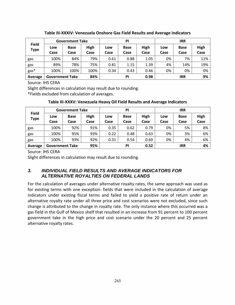
265

Table III-XXXIV: Venezuela Onshore Gas Field Results and Average Indicators

Field Type


Low Case

Base Case

High Case

Low Case

Base Case

High Case

Low Case

Base Case

High Case

gas 100% 84% 79% 0.61 0.88 1.05 0% 7% 11%

gas 89% 78% 75% 0.81 1.15 1.39 4% 14% 19%

gas* 100% 100% 100% 0.34 0.43 0.46 0% 0% 0%



Table III-XXXV: Venezuela Heavy Oil Field Results and Average Indicators

Field Type


Low Case

Base Case

High Case

Low Case

Base Case

High Case

Low Case

Base Case

High Case

gas 100% 92% 91% 0.35 0.62 0.79 0% 5% 8%

gas 100% 95% 93% 0.22 0.48 0.63 0% 3% 6%

gas 100% 93% 92% 0.31 0.54 0.69 0% 4% 6%


PI 0.52

IRR 4%


3. INDIVIDUAL FIELD RESULTS AND AVERAGE INDICATORS FOR ALTERNATIVE ROYALTIES ON FEDERAL LANDS

For the calculation of averages under alternative royalty rates, the same approach was used as for existing terms with one exception: fields that were included in the calculation of average indicators under existing fiscal terms and failed to yield a positive rate of return under an alternative royalty rate under all three price and cost scenarios were not excluded, since such change is attributed to the change in royalty rate. The only instance where this occurred was a gas field in the Gulf of Mexico shelf that resulted in an increase from 91 percent to 100 percent government take in the high price and cost scenario under the 20 percent and 25 percent alternative royalty rates.

266

Table III-XXXVI: Gulf of Mexico Deepwater Results and Average Indicators—12.5 Percent Alternative Royalty

12.5% Royalty

Field Type


Low Case

Base Case

High Case

Low Case

Base Case

High Case

Low Case

Base Case

High Case

gas* 100% 100% 100% 0.21 0.36 0.43 0% 0% 0%

gas 100% 71% 60% 0.55 0.83 0.95 0% 4% 8%

gas* 100% 100% 100% 0.24 0.39 0.47 0% 0% 0%

gas* 100% 100% 100% 0.07 0.15 0.19 0% 0% 0%

gas* 100% 100% 100% 0.03 0.05 0.07 0% 0% 0%

oil 57% 49% 47% 0.86 1.28 1.52 7% 15% 19%

oil 54% 48% 47% 0.90 1.35 1.61 8% 16% 19%

oil 54% 48% 47% 0.89 1.31 1.54 8% 15% 19%

oil 61% 50% 48% 0.78 1.15 1.35 5% 13% 17%

oil 61% 50% 48% 0.74 1.10 1.30 4% 12% 15%



Table III-XXXVII: Gulf of Mexico Deepwater Results and Average Indicators—20 Percent Alternative Royalty

20% Royalty

Field Type


Low Case

Base Case

High Case

Low Case

Base Case

High Case

Low Case

Base Case

High Case

gas* 100% 100% 100% 0.19 0.32 0.38 0% 0% 0%

gas 100% 89% 73% 0.49 0.77 0.88 0% 2% 6%

gas* 100% 100% 100% 0.22 0.36 0.43 0% 0% 0%

gas* 100% 100% 100% 0.05 0.13 0.16 0% 0% 0%

gas* 100% 100% 100% 0.03 0.05 0.06 0% 0% 0%

oil 70% 57% 55% 0.79 1.18 1.40 5% 14% 17%

oil 65% 56% 54% 0.82 1.24 1.48 6% 14% 18%

oil 65% 56% 54% 0.82 1.20 1.42 6% 14% 17%

oil 77% 58% 56% 0.72 1.06 1.25 3% 11% 15%

oil 76% 58% 56% 0.68 1.01 1.20 3% 10% 14%



267

Table III-XXXVIII: Gulf of Mexico Deepwater Results and Average Indicators—25 Percent Alternative Royalty

25% Royalty

Field Type


Low Case

Base Case

High Case

Low Case

Base Case

High Case

Low Case

Base Case

High Case

gas* 100% 100% 100% 0.17 0.30 0.36 0% 0% 0%

gas 100% 100% 81% 0.45 0.73 0.84 0% 0% 4%

gas* 100% 100% 100% 0.20 0.33 0.39 0% 0% 0%

gas* 100% 100% 100% 0.04 0.11 0.15 0% 0% 0%

gas* 100% 100% 100% 0.02 0.04 0.05 0% 0% 0%

oil 78% 62% 59% 0.75 1.11 1.32 4% 12% 16%

oil 73% 61% 58% 0.78 1.17 1.39 5% 13% 17%

oil 73% 61% 59% 0.77 1.14 1.34 5% 13% 16%

oil 88% 64% 61% 0.67 1.00 1.18 2% 10% 14%

oil 86% 64% 61% 0.64 0.95 1.13 2% 9% 12%



Table III-XXXIX: Gulf of Mexico Deepwater Results and Average Indicators—Sliding Scale Alternative Royalty


Field Type


Low Case

Base Case

High Case

Low Case

Base Case

High Case

Low Case

Base Case

High Case

gas* 100% 100% 100% 0.19 0.31 0.36 0% 0% 0%

gas 100% 90% 80% 0.51 0.77 0.85 0% 1% 4%

gas* 100% 100% 100% 0.19 0.32 0.38 0% 0% 0%

gas* 100% 100% 100% 0.06 0.13 0.16 0% 0% 0%

gas* 100% 100% 100% 0.01 0.03 0.04 0% 0% 0%

oil 65% 56% 57% 0.82 1.19 1.36 6% 14% 17%

oil 61% 55% 56% 0.85 1.26 1.44 7% 15% 17%

oil 63% 54% 53% 0.83 1.22 1.44 6% 14% 17%

oil 73% 58% 59% 0.72 1.05 1.20 3% 11% 14%

oil 77% 60% 60% 0.66 0.98 1.13 2% 10% 12%



268

Table III-XL: Gulf of Mexico Shelf Results and Average Indicators—12.5 Percent Alternative Royalty

12.5% Royalty

Field Type


Low Case

Base Case

High Case

Low Case

Base Case

High Case

Low Case

Base Case

High Case

gas 100% 100% 73% 0.25 0.44 0.52 0% 0% 1%

gas 78% 53% 50% 0.62 0.86 0.98 1% 7% 10%

gas 65% 51% 49% 0.75 1.09 1.28 4% 12% 16%

gas* 100% 100% 100% 0.19 0.44 0.56 0% 0% 0%

gas* 100% 100% 100% 0.01 0.19 0.27 0% 0% 0%

gas* 100% 100% 100% 0.00 0.09 0.14 0% 0% 0%

gas* 100% 100% 100% 0.00 0.00 0.01 0% 0% 0%

oil 100% 54% 51% 0.57 0.89 1.06 0% 8% 11%

oil 100% 70% 58% 0.50 0.80 0.93 0% 3% 8%

oil* 100% 100% 100% 0.33 0.56 0.68 0% 0% 0%



Table III-XLI: Gulf of Mexico Shelf Results and Average Indicators—20 Percent Alternative Royalty

20% Royalty

Field Type


Low Case

Base Case

High Case

Low Case

Base Case

High Case

Low Case

Base Case

High Case

gas 100% 100% 95% 0.21 0.40 0.47 0% 0% 0%

gas 100% 63% 59% 0.58 0.80 0.92 0% 6% 8%

gas 82% 60% 57% 0.69 1.01 1.18 2% 10% 14%

gas* 100% 100% 100% 0.14 0.35 0.48 0% 0% 0%

gas* 100% 100% 100% -0.02 0.14 0.22 0% 0% 0%

gas* 100% 100% 100% -0.02 0.06 0.11 0% 0% 0%

gas* 0% 0% 100% 0.00 0.00 0.01 0% 0% 0%

oil 100% 65% 60% 0.50 0.82 0.97 0% 6% 10%

oil 100% 90% 71% 0.45 0.75 0.87 0% 1% 6%

oil* 100% 100% 100% 0.29 0.50 0.62 0% 0% 0%



269

Table III-XLII: Gulf of Mexico Shelf Results and Average Indicators—25 Percent Alternative Royalty

25% Royalty

Field Type


Low Case

Base Case

High Case

Low Case

Base Case

High Case

Low Case

Base Case

High Case

gas 100% 100% 100% 0.19 0.36 0.44 0% 0% 0%

gas 100% 70% 65% 0.54 0.76 0.87 0% 5% 7%

gas 93% 66% 62% 0.65 0.95 1.11 1% 9% 12%

gas* 100% 100% 100% 0.11 0.31 0.40 0% 0% 0%

gas* 0% 100% 100% 0.00 0.11 0.18 0% 0% 0%

gas* 100% 100% 100% -0.11 0.04 0.08 0% 0% 0%

gas* 0% 0% 100% 0.00 0.00 0.00 0% 0% 0%

oil 100% 72% 66% 0.45 0.77 0.92 0% 5% 8%

oil 100% 100% 80% 0.41 0.70 0.82 0% 0% 4%

oil* 100% 100% 100% 0.27 0.46 0.57 0% 0% 0%



Table III-XLIII: Gulf of Mexico Shelf Results and Average Indicators—Sliding Scale Alternative Royalty


Field Type


Low Case

Base Case

High Case

Low Case

Base Case

High Case

Low Case

Base Case

High Case

gas 100% 100% 100% 0.23 0.40 0.46 0% 0% 0%

gas 92% 61% 61% 0.60 0.81 0.90 0% 6% 8%

gas 76% 60% 60% 0.71 1.01 1.14 3% 10% 13%

gas* 100% 100% 100% 0.11 0.31 0.42 0% 0% 0%

gas* 100% 100% 100% -0.01 0.15 0.19 0% 0% 0%

gas* 100% 100% 100% -0.01 0.06 0.09 0% 0% 0%

gas* 100% 100% 100% -0.02 0.00 0.00 0% 0% 0%

oil 100% 65% 64% 0.29 0.82 0.94 0% 6% 9%

oil 100% 91% 78% 0.47 0.75 0.84 0% 1% 4%

oil* 100% 100% 100% 0.27 0.45 0.53 0% 0% 0%



270

Table III-XLIV: Wyoming Results and Average Indicators—18.75 Percent Alternative Royalty

18.75% Royalty

Field Type


Low Case

Base Case

High Case

Low Case

Base Case

High Case

Low Case

Base Case

High Case

gas 68% 60% 59% 1.35 2.13 2.59 19% 40% 50%

gas* 100% 100% 100% -0.02 0.03 0.08 0% 0% 0%

gas* 100% 100% 100% 0.22 0.40 0.50 0% 0% 0%

gas* 100% 100% 100% 0.09 0.20 0.27 0% 0% 0%

gas* 100% 100% 100% -0.04 0.05 0.12 0% 0% 0%

CBG 58% 54% 54% 1.16 1.97 2.37 12% 21% 24%

CBG 100% 83% 70% 0.24 0.48 0.58 0% 1% 3%

CBG 100% 66% 62% 0.49 0.86 1.02 0% 7% 10%

CBG 100% 65% 61% 0.55 0.96 1.14 0% 9% 13%

CBG 100% 65% 61% 0.54 0.94 1.11 0% 9% 12%

Average Government Take 71% PI 114 IRR 13%


Table III-XLV: Wyoming Results and Average Indicators—20 Percent Alternative Royalty

20% Royalty

Field Type


Low Case

Base Case

High Case

Low Case

Base Case

High Case

Low Case

Base Case

High Case

gas 69% 61% 60% 1.27 2.10 2.55 19% 39% 49%

gas* 100% 100% 100% -0.02 0.03 0.07 0% 0% 0%

gas* 100% 100% 100% 0.22 0.40 0.49 0% 0% 0%

gas* 100% 100% 100% 0.09 0.20 0.27 0% 0% 0%

gas* 100% 100% 100% -0.04 0.05 0.11 0% 0% 0%

CBG 58% 55% 54% 1.15 1.94 2.34 12% 21% 24%

CBG 100% 85% 72% 0.24 0.47 0.57 0% 1% 3%

CBG 100% 68% 63% 0.48 0.84 1.00 0% 7% 10%

CBG 100% 66% 62% 0.54 0.94 1.12 0% 9% 13%

CBG 100% 67% 63% 0.53 0.93 1.10 0% 8% 12%



271

Table III-XLVI: Wyoming Results and Average Indicators—25 Percent Alternative Royalty

25% Royalty

Field Type


Low Case

Base Case

High Case

Low Case

Base Case

High Case

Low Case

Base Case

High Case

gas 74% 66% 64% 1.19 1.96 2.37 16% 36% 45%

gas* 100% 100% 100% -0.02 0.02 0.05 0% 0% 0%

gas* 100% 100% 100% 0.20 0.36 0.45 0% 0% 0%

gas* 100% 100% 100% 0.07 0.18 0.24 0% 0% 0%

gas* 100% 100% 100% -0.04 0.04 0.09 0% 0% 0%

CBG 62% 58% 58% 1.10 1.84 2.21 11% 20% 23%

CBG 100% 94% 78% 0.22 0.45 0.54 0% 0% 2%

CBG 100% 73% 75% 0.45 0.80 0.95 0% 6% 9%

CBG 100% 71% 67% 0.50 0.89 1.06 0% 8% 11%

CBG 100% 72% 67% 0.49 0.87 1.04 0% 7% 11%



Table III-XLVII: Wyoming Results and Average Indicators—Sliding Scale Alternative Royalty


Field Type


Low Case

Base Case

High Case

Low Case

Base Case

High Case

Low Case

Base Case

High Case

Gas 62% 57% 58% 1.40 2.24 2.74 22% 42% 50%

gas* 100% 100% 100% -0.02 0.06 0.10 0% 0% 0%

gas* 100% 100% 100% 0.25 0.46 0.55 0% 0% 0%

gas* 100% 100% 100% 0.10 0.25 0.31 0% 0% 0%

gas* 100% 100% 100% -0.04 0.09 0.15 0% 0% 0%

CBG 53% 50% 52% 1.22 2.10 2.43 13% 22% 25%

CBG 100% 73% 67% 0.25 0.51 0.59 0% 2% 3%

CBG 100% 59% 60% 0.54 0.91 1.04 0% 8% 11%

CBG 93% 58% 59% 0.47 1.02 1.16 0% 10% 9%

CBG 98% 59% 59% 0.59 1.00 1.14 0% 10% 13%



272

APPENDIX IV—CHANGES IN FISCAL TERMS OVER THE PAST FIVE YEARS

Alaska

In 2006, the government introduced proposed legislation to eliminate the production tax called ELF (Economic Limit Factor) and replace it with a petroleum profits tax (PPT). The PPT which came into force in April 2007, was replaced in November 2007 by another profits tax called ACES (Alaska’s Clear and Equitable Share). The application of ACES, which was levied on existing as well as future production, was made retroactive to July 1, 2007. This change led to an increase of government take by 17 percent compared to that under ELF (ELF was a severance tax linked to the economic limit of the field).

Alberta Conventional

In 2007, the government of Alberta introduced a new royalty framework that resulted in the increase of the maximum royalty rate for crude oil from 30 percent to 50 percent. The new royalty rate, which was supposed to enter into effect in 2009, was never implemented. As a result of the drop in oil prices and the global economic crises, the government suspended the implementation of the new royalty framework for a one-year period. Subsequently, the government introduced several incentives to halt the drop in drilling activity. In January 2011, the government permanently suspended the 2007 royalty framework and introduced a new royalty rate with a cap at 40 percent for crude oil and 36 percent for natural gas. The new royalty framework applies to existing as well as future production.

Alberta’s 2011 terms for conventional oil were compared against the fiscal terms for “third tier oil” as they applied prior to the introduction of the 2007 royalty framework. 216 Such a change led to 9 percent increase in government take, from 39 percent to 48 percent.

Alberta Oil Sands

In 2007, the government increased the royalty rate for oil sands projects. The royalty rate consists of a gross revenue and a net revenue component. The gross revenue was increased from 1 percent to 9 percent. The net revenue was increased from 25 percent to a sliding scale of 25–40 percent when WTI oil prices ranged between C$55 and C$120 per barrel. This led to an 18 percent increase in government take, from 45 to 63 percent.

Algeria

In 2005, the government of Algeria changed completely the legal framework from a PSA type of right to a concessionary one. The change released the national oil company from any regulatory authority and eliminated the mandatory national oil company participation in PSAs. In 2006, however, the government introduced a 50 percent mandatory national oil company participation for new licenses, as well as a windfall profits tax for existing PSAs. The change led to a 16 percent increase in government take, from 67 to 83 percent, for new acreage.

216

Oil discovered after September 1, 1992.

273

Angola

In the 2006 and 2007 bidding rounds, Angola lowered the rate of return thresholds for applying the sliding scale profit sharing, which led to a 9 percent increase of the government take, from 82 to 91 percent, for profitable projects.

Fiscal System IRR Contractor Profit Sharing

Pre-2006 0% 60%

20% 50%

25% 40%

30% 30%

Post-2006 10% 70%

13% 55%

18% 45%

20% 30%

>20% 20%

Source: IHS CERA

Australia

In 2008, the Australian government passed the Excise Tariff Amendment (Condensate) Act 2008, which amended the Excise Tariff Act 1921 by applying the excise system for oil-to-condensate effective from May 13, 2008. Previously, excise on the production of condensate did not apply to the Northwest Shelf project (in federal waters), state waters, and onshore (i.e., areas not subject to the federal Petroleum Resource Rent Tax).

Brazil

On December 22, 2010, Brazil passed Law No. 12,351, which governs the pre-salt legal system and amends several provisions of the 1997 Petroleum Law. Under the new law, PSAs are prescribed as one of the possible contractual arrangements in Brazil. Under the PSA system, Petrobras will act as sole operator, with a minimum 30 percent mandatory participation in all PSAs signed for pre-salt areas or “strategic” areas as designated by the National Petroleum Policy Council. Petrobras has the right, either solely or in consortium with other partners, to conduct all the exploration and production operations required within the pre-salt blocks, at its cost and risk, and, in the event of a commercial discovery, be entitled to reimbursement of the costs incurred (cost oil) and a share of the surplus production (profit oil).

The terms modeled for this study pertain to the concessionary system in existence prior to the passage of Law No. 12,351. The model PSA had not been released at the time this report was written. However, the minimum 30 percent state participation was modeled under the concessionary system to determine the likely increase in government take. Such a measure, if applied under the existing concessionary system, will result in a 12 percent increase in government take, from 59 percent to 71 percent, in the case of profitable oil fields.

274

British Columbia

British Columbia introduced a net revenue royalty for shale gas in 2008, which led to a 24 percent drop in government take, from 62 to 38 percent.

China

In 2006, China introduced a windfall profits tax that applies when crude oil prices exceed $40 per barrel. In the same year, China introduced a 5 percent export duty. Offshore operators were exempt until 2012. The government take increased by 4 percent, from 70 to 74 percent, for highly profitable oil fields.

Colombia

In 2007, Colombia introduced a new levy called “ANH production participation,” which is effectively an additional royalty. The percentage is a biddable item and has varied from 2 percent to 32 percent. On average, government take increased by 13 percent, from 62 to 75 percent.

Germany

In 2006, corporate income tax was increased from 38.31 percent, to 38.34 percent. In 2008, Germany reduced corporate income tax to 25 percent.

India

In its 2006/2007 budget, the Indian government announced an increase in the rate of Minimum Alternate Tax from 7.5 percent of book profits to 10 percent.217 In September 2009, Finance Act (No. 2) of 2009 reinstated the seven-year tax holiday on natural gas for blocks to be awarded under New Exploration Licensing Policy (NELP) VIII (the government withdrew the seven-year tax holiday for gas producers in 2008 but retained the tax holiday for oil production). This change to the tax holiday is not retroactive and is effective for gas production commencing on or after April 1, 2009, only under NELP VIII and Coal Bed Methane (CBM) IV.

Indonesia Coalbed Gas

In 2008, the government introduced incentives for coalbed gas projects, which consisted of:

reduction of first tranche petroleum from 20 to 10 percent

increase of contractor after-tax profit share from 40 percent to 45 percent

Indonesia Conventional

Indonesia has frequently changed the first tranche petroleum over the past few years. In 2006, the first tranche was reduced from 20 percent to 10 percent. In 2009, the first tranche was increased back to the original 20 percent rate applicable prior to 2006. Such changes were limited to future contracts.

In June 2008, the government moved to make certain costs not recoverable with the issue

217

This increase has not affected the result of our models since the corporate income tax liability has been greater than MAT.

275

of Regulation No. 22 on Types of Costs not Subject to Reimbursement. This was seen as a tightening of the cost recovery process. Costs no longer permissible include personal income taxes, and losses on private car and house sales long-term incentive plans hiring expatriates without work permits hiring legal consultants for unrelated legal matters tax consultant fees costs of oil and gas marketing that are a result of contractor's mistakes public relations events without lists of attendees community development costs restoration site funds technical training of expatriates merger or acquisition costs borrowing costs third-party income taxes procurement of goods and services for amounts larger than authorizations of

expenditure (based on government calculations) assets that have been placed into service but are not functioning transactions with affiliated parties that inflict losses on the state

These restrictions were to apply to existing and future contracts and would require improved monitoring of contracts in a bid to reduce alleged cost recovery abuse.

Kazakhstan

In 2008, royalty tax arrangements were introduced for offshore acreage resulting in a lowering of the government take by 14 percent when compared to production sharing terms applicable previously. While the 2008 change has resulted in an overall reduction of the government take, the fiscal system applicable to oil and gas investment has undergone frequent changes, which have as a consequence resulted in a rather unstable fiscal system. The following are some of the changes introduced during the last five years:

2007: contract renegotiation and imposition of increased national oil company participation

2008:

o The tax code provided for

gradual reduction of income tax from 20 percent in 2009 to 17.5 percent in 2010 and 15 percent in 2011

gradual increase of the mineral extraction tax from a range of 5–18 percent in 2009 to a range of 6–19 percent in 2010 and 7–20 percent in 2011

o Export duties:

June 2008—Export duty on crude oil and gas condensate was introduced at a rate of US$109.91 per ton (US$27.43 per ton applying to companies

276

already paying the export rent tax).

October 2008—The rate of duty was increased to US$203.8 per ton (US$121.32 for companies already paying the export rent tax).

2009:

o Falling crude oil prices in 2008 led the government to announce a reduction in the rate of export duty to US$139.79 (US$57.31 for companies already paying the export rent tax) effective on January 20, 2009, and at the same time an undertaking to review the rate of duty on a monthly basis as opposed to the previously applicable quarterly basis.

o With oil prices continuing to fall, the rate of export duty was set at zero effective on January 26, 2009 (prior to that, a government decree signed on December 24, 2008 had exempted companies paying the export rent tax on crude oil from the export duty levy with effect from January 1, 2009).

2010:

o The tax code was amended as follows:

The 20 percent corporate income tax rate applies through December 31, 2012; then is reduced to 17.5 percent in 2013 and 15 percent in 2014.

Since the corporate income tax rate for 2010–2012 remained at the 2009 level, the mineral extraction rate for 2010–2012 will also remain at the 2009 range between 5–18 percent and will not increase until 2013. In 2013, the range of the mineral extraction tax is expected to be between 6 and 19 percent and in 2014 between 7 and 20 percent.

o On August 16, 2010, the government reinstated export duty on crude oil at the rate of US$20 per ton through Government Resolution No. 709 of July 13, 2010.

2011

o An announcement from the Ministry of Finance about an intention to increase the duty rate so as to boost state budget revenues followed in September 2010, and the rate of export duty on crude oil was raised to US$40 per ton effective January 1, 2011, pursuant to Government Resolution No. 1445 of December 30, 2010.

Libya

In 2005–2006, Libya introduced Exploration and Production Sharing Agreements (EPSA) IV model contract. Competition for acreage in Libya led to a 28 percent increase of government take compared with EPSA III terms. Although this shift was driven by market forces, the government used it to renegotiate existing contracts to bring them in line with bids under EPSA IV.

277

Louisiana

No change.

Malaysia

No change.

Norway

No change.

Poland

In 2007, the crude oil royalty rate was increased from $1.18 to $1.57 per barrel and from $0.042 to $0.053 per Mcf.

Queensland

From July 1, 2012, Petroleum Resources Rent Tax (PRRT) as currently applies to offshore projects is proposed to apply to all onshore oil, gas, and coal steam projects and the offshore Northwest Shelf project. This will lead to an increase in government take of 26 percent.

Russia

Over the past five years, the Russian government has introduced various changes affecting its oil and gas fiscal systems. The following is a summary of changes in chronological order:

2006: o On July 27, 2006, Law No. 137-FZ was passed establishing a zero Mineral

Production Tax rate for new oil deposits in all new oil fields in Siberia's Yakutia Republic and the Irkutsk and Krasnoyarsk regions. In addition, differentiated (i.e., discounted) rates of MPT were introduced for oil fields that are at least 80 percent depleted. These measures, which entered into force on January 1, 2007, were designed to encourage oil companies to invest in new deposits in less accessible areas and to employ enhanced technology to prolong the production life of older deposits. These measures were to remain in force for 10 years for crude oil and natural gas production licenses and 15 years for exploration and production licenses but may be withdrawn ahead of time where a field's cumulative production exceeds 25 million tons.

2008: o Law No. 158-FZ of July 22, 2008 increased the nontaxable Urals price threshold

for the purposes of calculating MPT from US$9 to US$15 per barrel. Law No. 158-FZ introduced tax exemptions for selected projects until cumulative production reaches the specified level indicated below:218

in the northern Timan-Pechora: up to 35 million tons of cumulative production

in the Yamal/Nenets oil provinces: up to 15 million tons of cumulative

218

Tax exemptions were effective on 1 January 2009.

278

production in the Caspian and Azov Seas: up to 10 million tons of cumulative

production o Law No. 224-FZ of November 28, 2008, was introduced as part of Russia's

response to the global financial crisis. The law included, among other things, a number of measures favoring taxpayers, including a reduction in the rate of corporate profits tax from 24 to 20 percent.

2009: o In July 2009, the government announced further MPT tax exemptions for

offshore projects in the Black Sea and the Sea of Okhotsk in eastern Russia. Under these exemptions, fields will enjoy a zero rate of MPT for a period of 10 to 15 years (depending on license type) or until cumulative production reaches 20 million tons for Black Sea fields or 30 million tons for fields in the Sea of Okhotsk. These provisions apply to licenses granted from and including January 2009.

2010: o From December 8, 2010, two further fields were added to the list of 22 fields

that benefit from a reduced rate of export duty. The two fields are Lukoil’s Yuri Korchagin field and Vladimir Filanovsky field, both in the North Caspian.

2011: o Mineral Production Tax:

On January 1, 2011, new rates of MPT applicable to oil production and gas production from gas deposits (i.e., nonassociated gas) were introduced. For the period 2011 to 2013, the new rates are to change in line with forecast inflation. As a result government take is expected to increase by 11 percent.

The new rates for oil are: o 2011: RUR 419 per ton, o 2012: RUR 446 per ton o 2013: RUR 470 per ton

The new rates for gas are o 2011: RUR 237 per 1,000 cubic meters o 2012: RUR 251 per 1,000 cubic meters o 2013: RUR 265 per 1,000 cubic meters.

Government Decree No. 311 of April 25, 2011, specifies that, with effect from May 1, 2011, Vankorskoye, Verkhnechonskoye, and Talakanskoye fields no longer qualified for the export duty incentives, and the regular duty rate would be applicable to exports of crude oil produced from these fields.

Effective June 1, 2011, Vankorskoye field (operated by Rosneft) is back onto the list of designated East Siberian fields that qualify for the reduced export duty rate.

279

o Export duties: The rate of export duty is set by the Russian government on a monthly basis. Between January and June 2011, the export duty increased by 46 percent:

January 2011: US$317 per ton February 2011: US$346 per ton March 211: US$365 per ton April 2011: US$423.7 per ton May 2011: US$453.7 per ton June 211: US$462.1 per ton219

o Proposed changes: The Russian government is planning to introduce the following changes to the MPT:220

Incentives for small oil fields:

The formula for the MPT rate will be amended to read as follows: MPT = K * Cp * Cd * Cr

where Cr is a new factor reflecting the size of reserves (“reserves coefficient”) (K, Cp and Cd will remain unchanged). For oil fields with initial recoverable reserves of less than 5 million tons (36.5 million barrels*), Cr will be calculated as follows, as long as the cumulative production does not exceed 5 percent of the reserves:

Cr = 0.125 * R + 0.375 where R = initial recoverable reserves (million tons). If initial recoverable reserves equal to or greater than 5 million tons (36.5 million barrels*) and/or cumulative production exceeds 5 percent of the reserves size, Cr will be equal to 1.0.

Incentives for oil fields in northern Yamal-Nenets region:

Oil fields of Yamal-Nenets autonomous region, which are located above 65 degrees North, will enjoy a zero rate of MPT for a period of 10 to 15 years (depending on license type, date of its issue, and the level of reserves depletion) or until cumulative production reaches 25 million tons (182.5 million barrels).*

Texas

No change.

United Kingdom

During the past five years the U.K. government has introduced measures that led to an increase of the government take as well as incentives to encourage production from small fields. The

219

June 2011 rate represents the highest level since a record $495.90 per ton in August and September 2008. According to Bloomberg, on July 1, 2011, the export duty is expected to fall between $443.20 and $445.30 per metric ton. 220

The proposed measures will be introduced via amendments to Article 342 of Part Two of the Tax Code. The respective draft laws are currently being discussed by State Duma. It is expected the laws will be adopted before the end of 2011.

280

following changes were introduced in chronological order:

2006: The rate of special petroleum tax was increased from 10 percent to 20 percent.

2009: Certain fields given development approval on or after April 22, 2009, benefit from a field allowance that is deductible from the taxable income subject to a special petroleum tax. The field allowance is a fixed amount per company and is subject to an annual limit. It applies to selected types of fields; this study considers only the field allowance for small fields, which is £75 million for fields with recoverable reserves <2.75 million tons of oil equivalent (US$112.5 million for reserves <20.075MMboe) reducing on a straight-line basis to £0 for fields with recoverable reserves >3.5 million tons of oil equivalent (US$0 for reserves >25.55 MMboe). The maximum annual allowance is £15 million (US$22.5 million).

2011: The U.K. government increased the special petroleum tax from 20 percent to 32 percent.

The changes introduced since 2006 have led to a 22 percent increase of the government take for fields developed after 1992.

U.S. Gulf of Mexico Deepwater

During the past five years, the U.S. DOI introduced measures that led to an increase in royalty rates and rentals in deepwater areas of the Gulf of Mexico region. The measures, which applied only to future lease sales, resulted in 8 percent overall increase of government take of specific fields.

2007: Increase of royalty rate from 12.5 percent to 16.67 percent was announced on January 9, 2007, and took effect with Western Gulf of Mexico lease sale 204 on August 22, 2007.

2008: The royalty rate was increased from 16.67 percent to 18.75 percent on March 19, 2008, in relation to lease sales 206 and 244 in Central Gulf of Mexico and Eastern Gulf of Mexico, respectively.

2009: Increase of rental rates from $7.50 per acre to $11–$44 per acre for water depths between 200 and 400 meters and to $11–$16 per acre for water depths of 400 meters and greater, was introduced on March 18, 2009, in association with Central Gulf of Mexico lease sale 208.

U.S. Gulf of Mexico Shelf

During the past five years, the U.S. DOI introduced measures that led to an increase in royalty rates and rentals in shelf areas of the Gulf of Mexico region. The measures, which applied only to future lease sales, resulted in a 3 percent overall increase of government take of specific fields. The following changes were introduced in this period:

2008: The royalty rate was increased from 16.67 percent to 18.75 percent on March 19, 2008, in relation to lease sales 206 and 244 in Central Gulf of Mexico and Eastern Gulf of Mexico, respectively.

2009: Increase of rental rates from $5 per acre to $7–$28 per acre for water depths up

281

to 200 meters was introduced on March 18, 2009, in association with Central Gulf of Mexico lease sale 208.

Venezuela Conventional Gas

No change.

Venezuela Heavy Oil

Since 2005, Venezuela took various measures to increase state control over natural resources. The following measures apply to extra heavy oil projects:

2005: termination of royalty rate reduction eligibility, which resulted in an increase of royalty rate from 1to 16.67 percent

2006: o increase of royalty rate from 16.6 to 30 percent o increase of income tax from 34 to 50 percent o introduction of extraction tax of 33.33 percent (effectively 3.33 percent)

2007:

o renegotiation of existing agreements o introduction of 60 percent mandatory PDVSA (national oil company)

participation

2008:

o introduction of windfall profits tax levied at a rate of 50 percent on oil revenues (from the export of liquid hydrocarbons and their products) between a Brent oil price of US$70 per barrel and US$100 per barrel, and at a rate of 60 percent of revenues above a Brent oil price of US$100 per barrel

2011:

o Amendment to Windfall Profits Tax. On April 18, 2011, a Decree Creating a Special Contribution on Extraordinary and Exorbitant Prices in the International Hydrocarbons Market (the Special Contribution), was passed. The decree describes two types of prices: “extraordinary prices” and “exorbitant prices.”

“Extraordinary price” is defined as the monthly average price of the Venezuelan hydrocarbons basket when this is higher than the price established in the Annual Budget Law (currently US$40 per barrel) but equal to or less than US$70 per barrel. In this case, the Special Contribution rate will be 20 percent of the difference between both prices.

“Exorbitant price” is defined as the monthly average price of the Venezuelan hydrocarbons basket when this is higher than US$70 per barrel. In this case, the Special Contribution has different rates:

When the price is more than US$70 per barrel but less than US$90

282

per barrel the rate will be 80 percent of the price differential.

When the price is more than US$90 per barrel but less than US$100 per barrel the rate will be 90 percent of the price differential.

When the price is equal to or higher than US$100 per barrel the rate will be 95 percent of US$100 and the average price equal to or above this baseline.

Projects for the development of new reservoirs and those ongoing projects aimed at increasing production are exempted from the Special Contribution as long as they have not recovered their investments.

Wyoming Federal Lands No change.

283

APPENDIX V—INDEX TABLES

Table V-I: Fiscal Terms Index (Unweighted Score)

Fiscal System Gov Take

Index

Score PI

Index Score

IRR Index Score

Progresivity/ Regressivity

Index Score

Algeria onshore 86% 4.32 1.83 0.00 25% 0.43 -9% 1.50

Angola offshore 78% 3.70 1.32 1.93 16% 2.27 2% 0.17

Australia (Queensland) coalbed gas 40% 0.89 1.41 1.60 15% 2.56 -10% 1.67

Australia offshore 71% 3.18 1.57 0.99 20% 1.50 -8% 1.33

Brazil offshore 72% 3.28 1.62 0.80 14% 2.78 -22% 3.67

Canada (Alberta) conventional oil 61% 2.49 1.32 1.93 16% 2.45 -30% 5.00

Canada (Alberta) oil sands 67% 2.91 1.10 2.78 9% 3.85 -19% 3.17

Canada (British Columbia) 40% 0.87 1.17 2.52 13% 2.97 1% 0.16

China offshore 80% 3.88 1.46 1.41 12% 3.20 8% 1.21

Colombia onshore 82% 4.03 1.20 2.40 16% 2.35 -4% 0.67

Germany onshore 61% 2.46 0.80 3.92 6% 4.49 -11% 1.83

India offshore 57% 2.16 1.23 2.28 15% 2.56 -16% 2.67

Indonesia coalbed gas 79% 3.78 1.35 1.81 23% 0.76 -12% 2.00

Indonesia conventional gas offshore 82% 4.00 1.07 2.91 11% 3.38 -13% 2.17

Kazakhstan offshore 78% 3.73 1.17 2.51 13% 2.99 9% 1.33

Libya onshore 91% 4.66 1.43 1.51 17% 2.09 4% 0.52

Malaysia offshore 93% 4.85 0.93 3.42 7% 4.27 -12% 2.00

Norway offshore 79% 3.79 1.04 3.02 12% 3.28 27% 4.50

Poland onshore 28% 0.00 1.50 1.26 16% 2.35 -8% 1.33

Russia onshore 73% 3.36 1.26 2.17 14% 2.78 -22% 3.67

United Kingdom offshore 62% 2.53 1.13 2.66 12% 3.20 0% 0.00

U.S. Alaska onshore 76% 3.59 1.09 2.81 11% 3.36 -18% 3.00

U.S. GOM deepwater 64% 2.65 1.04 3.01 10% 3.64 -18% 3.00

U.S. GOM shelf 79% 3.77 0.72 4.23 4% 4.83 -16% 2.67

U.S. Louisiana onshore gas 85% 4.27 1.03 3.05 27% 0.00 -9% 1.50

U.S. Texas onshore 76% 3.55 0.95 3.35 11% 3.42 -17% 2.83

U.S. Wyoming gas 66% 2.85 1.22 2.33 14% 2.81 -17% 2.67

Venezuela conventional gas 84% 4.18 0.98 3.22 9% 3.78 -13% 2.17

Venezuela heavy oil 95% 5.00 0.52 5.00 4% 5.00 -5% 0.83

Alternative Federal Fiscal Systems

U.S. GOM deepwater 12.5% royalty 55% 2.01 1.11 2.74 11% 3.32 -14% 2.33

U.S. GOM deepwater 20% royalty 65% 2.76 1.02 3.08 10% 3.68 -17% 2.83

U.S. GOM deepwater 25% royalty 72% 3.28 0.96 3.31 8% 3.93 -18% 3.00

U.S. GOM deepwater sliding scale royalty 65% 2.79 1.02 3.08 10% 3.71 -7% 1.17

U.S. GOM shelf 12.5% royalty 70% 3.13 0.77 4.03 5% 4.58 -13% 2.17

284

Fiscal System Gov Take

Index

Score PI

Index Score

IRR Index Score

Progresivity/ Regressivity

Index Score

U.S. GOM shelf 20% royalty 80% 3.88 0.71 4.27 4% 4.84 -17% 2.83

U.S. GOM shelf 25.5% royalty 85% 4.25 0.66 4.44 3% 5.00 -18% 3.00

U.S. GOM shelf sliding scale royalty 81% 3.92 0.69 4.33 4% 4.87 -6% 1.00

U.S. Wyoming gas 18.75% royalty 71% 3.24 1.14 2.63 13% 3.00 -17% 2.67

U.S. Wyoming gas 20% royalty 72% 3.31 1.12 2.71 13% 3.06 -17% 2.50

U.S. Wyoming gas 25% royalty 77% 3.62 1.05 2.96 11% 3.30 -16% 2.67

U.S. Wyoming gas sliding scale royalty 68% 2.96 1.19 2.45 13% 2.88 -13% 1.83

Source: IHS CERA

Table V-II: Fiscal Terms Index (Weighted Score)

Fiscal Terms Weighted Score

Fiscal System Weight Total Score 25% 25% 25% 25%

Gov Take

PI IRR Progressivity/ Regressivity

Algeria onshore 1.08 0.00 0.11 0.38 1.56

Angola offshore 0.93 0.48 0.57 0.04 2.02

Australia (Queensland) coalbed gas 0.22 0.40 0.64 0.42 1.68

Australia offshore 0.80 0.25 0.37 0.33 1.75

Brazil offshore 0.82 0.20 0.69 0.92 2.63

Canada (Alberta) conventional oil 0.62 0.48 0.61 1.25 2.97

Canada (Alberta) oil sands 0.73 0.69 0.96 0.79 3.17

Canada (British Columbia) 0.22 0.63 0.74 0.04 1.63

China offshore 0.97 0.35 0.80 0.33 2.45

Colombia onshore 1.01 0.60 0.59 0.17 2.36

Germany onshore 0.62 0.98 1.12 0.46 3.17

India offshore 0.54 0.57 0.64 0.67 2.42

Indonesia coalbed gas 0.95 0.45 0.19 0.50 2.09

Indonesia conventional gas offshore 1.00 0.73 0.84 0.54 3.11

Kazakhstan offshore 0.93 0.63 0.75 0.38 2.68

Libya onshore 1.17 0.38 0.52 0.17 2.23

Malaysia offshore 1.21 0.86 1.07 0.50 3.64

Norway offshore 0.95 0.75 0.82 1.13 3.65

Poland onshore 0.00 0.31 0.59 0.33 1.23

Russia onshore 0.84 0.54 0.69 0.92 2.99

United Kingdom offshore 0.63 0.67 0.80 0.00 2.10

U.S. Alaska onshore 0.90 0.70 0.84 0.75 3.19

U.S. GOM deepwater 0.66 0.75 0.91 0.75 3.08

285

Fiscal Terms Weighted Score


Gov Take


U.S. GOM shelf 0.94 1.06 1.21 0.67 3.88

U.S. Louisiana onshore gas 1.07 0.76 0.00 0.38 2.21

U.S. Texas onshore 0.89 0.84 0.85 0.71 3.29

U.S. Wyoming gas 0.71 0.58 0.68 0.67 2.64

Venezuela conventional gas 1.04 0.81 0.94 0.54 3.34

Venezuela heavy oil 1.25 1.25 1.25 0.21 3.96

Alternative Fiscal Systems

U.S. GOM deepwater 12.5% royalty 0.50 0.68 0.83 0.58 2.60

U.S. GOM deepwater 20% royalty 0.69 0.77 0.92 0.71 3.09


U.S. GOM deepwater sliding scale royalty 0.70 0.77 0.93 0.29 2.69

U.S. GOM shelf 12.5% royalty 0.78 1.01 1.15 0.54 3.48

U.S. GOM shelf 20% royalty 0.97 1.07 1.21 0.71 3.96


U.S. GOM shelf sliding scale royalty 0.98 1.08 1.22 0.25 3.53

U.S. Wyoming gas 18.75% royalty 0.81 0.66 0.75 0.67 2.88

U.S. Wyoming gas 20% royalty 0.83 0.68 0.76 0.63 2.89


U.S. Wyoming gas sliding scale royalty 0.74 0.61 0.72 0.46 2.53

Source: IHS CERA

Table V-III: Revenue Risk Index

Fiscal System Government Share of Total Benefit at 1/4 Field Life

Index Score

Algeria onshore 25% 1.80

Angola offshore 57% 5.00

Australia (Queensland) coalbed gas 26% 1.91

Australia offshore 29% 2.18

Brazil offshore 41% 3.44

Canada (Alberta) conventional oil 36% 2.87

Canada (Alberta) oil sands 37% 3.04

Canada (British Columbia) 13% 0.59

China offshore 32% 2.51

Colombia onshore 25% 1.85

Germany onshore 33% 2.61

India offshore 26% 1.86

286

Fiscal System Government Share of Total Benefit at 1/4 Field Life

Index Score

Indonesia coalbed gas 28% 2.15

Indonesia conventional gas offshore 14% 0.73

Kazakhstan offshore 34% 2.74

Libya onshore 27% 2.05

Malaysia offshore 25% 1.78

Norway offshore 7% 0.00

Poland onshore 16% 0.91

Russia onshore 41% 3.43

United Kingdom offshore 10% 0.28

U.S. Alaska onshore 55% 4.79

U.S. GOM deepwater 34% 2.71

U.S. GOM shelf 31% 2.38

U.S. Louisiana onshore gas 51% 4.39

U.S. Texas onshore 57% 4.95

U.S. Wyoming gas 45% 3.81

Venezuela conventional gas 56% 4.92

Venezuela heavy oil 36% 2.90

Alternative Federal Fiscal Systems

U.S. GOM deepwater 12.5% royalty 35% 2.81

U.S. GOM deepwater 20% royalty 34% 2.71

U.S. GOM deepwater 25% royalty 34% 2.71

U.S. GOM deepwater sliding scale royalty 33% 2.61

U.S. GOM shelf 12.5% royalty 29% 2.21

U.S. GOM shelf 20% royalty 31% 2.41

U.S. GOM shelf 25.5% royalty 32% 2.51

U.S. GOM shelf sliding scale royalty 31% 2.41

U.S. Wyoming gas 18.75% royalty 45% 3.80

U.S. Wyoming gas 20% royalty 45% 3.80

U.S. Wyoming gas 25% royalty 45% 3.80

U.S. Wyoming gas sliding scale royalty 43% 3.60

Source: IHS CERA

Table V-IV: Algeria Onshore—Timing of Government Revenue

Algeria

Field Type gas gas gas oil oil oil Gov Share of Benefit at 1/4 field life 21% 31% 28% 33% 16% 20%

Average 25%

Source: IHS CERA

287

Table V-V: Angola Offshore—Timing of Government Revenue

Angola

Field Type gas gas gas oil oil oil Gov Share of Benefit at 1/4 field life 47% 36% 98% 57% 60% 45% Average 57%

Source: IHS CERA

Table V-VI: Australia Offshore—Timing of Government Revenue

Australia Offshore

Field Type gas gas gas Gov Share of Benefit at 1/4 field life 25% 37% 24% Average 29%

Source: IHS CERA

Table V-VII: Australia (Queensland) Coalbed Gas—Timing of Government Revenue

Queensland


Source: IHS CERA

Table V-VIII: Brazil Offshore—Timing of Government Revenue

Brazil

Field Type gas gas gas oil oil oil

Gov Share of Benefit at 1/4 field life 52% 31% 37% 44% 43% 38% Average 41%

Source: IHS CERA

Table V-XIX: Canada (Alberta) Conventional Oil—Timing of Government Revenue

Alberta Conventional Oil

Field Type oil oil oil Gov Share of Benefit at 1/4 field life 33% 23% 51%

Average 36%

Source: IHS CERA

288

Table V-X: Canada (Alberta) Oil Sands—Timing of Government Revenue

Alberta Oil Sands

Field Type oil oil oil Gov Share of Benefit at 1/4 field life 33% 41% 38% Average 37%

Source: IHS CERA

Table V-XI: Canada (British Columbia)—Timing of Government Revenue

British Columbia


Source: IHS CERA

Table V-XII: China Offshore—Timing of Government Revenue

China


Source: IHS CERA

Table V-XIII: Colombia Onshore—Timing of Government Revenue

Colombia

Field Type gas gas gas oil oil oil


Source: IHS CERA

Table V-XIV: Germany Onshore—Timing of Government Revenue

Germany


Source: IHS CERA

289

Table V-XV: India Offshore—Timing of Government Revenue

India


Source: IHS CERA

Table: V-XVI: Indonesia Conventional Gas Offshore—Timing of Government Revenue

Indonesia Conventional Gas

Field Type gas gas gas Gov Share of Benefit at 1/4 field life 25% 23% 37%

Average 28%

Source: IHS CERA

Table V-XVII: Indonesia Coalbed Gas—Timing of Government Revenue

Indonesia Coalbed Gas

Field Type gas gas gas

Gov Share of Benefit at 1/4 field life 25% 8% 9% Average 14%

Source: IHS CERA

Table V- XVIII: Kazakhstan Offshore—Timing of Government Revenue

Kazakhstan

Field Type oil oil oil Gov Share of Benefit at 1/4 field life 42% 34% 27% Average 34%

Source: IHS CERA

Table V-XIX: Libya Onshore—Timing of Government Revenue

Libya


Source: IHS CERA

290

Table V-XX: Malaysia Offshore—Timing of Government Revenue

Malaysia


Source: IHS CERA

Table V-XXI: Norway Offshore—Timing of Government Revenue

Norway


Source: IHS CERA

Table V-XXII: Poland Offshore—Timing of Government Revenue

Poland

Field Type gas gas gas gas gas gas


Source: IHS CERA

Table V-XXIII: Russia Onshore—Timing of Government Revenue

Russia


Source: IHS CERA

Table V-XXIV: United Kingdom Offshore—Timing of Government Revenue

United Kingdom


Source: IHS CERA

291

Table: V-XXV: U.S. Alaska Onshore—Timing of Government Revenue

Alaska

Field Type gas gas gas oil oil oil Gov Share of Benefit at 1/4 field life 30% 50% 61% 51% 100% 40%

Average 55%

Source: IHS CERA

Table V-XXVI: U.S. Gulf of Mexico Deepwater—Timing of Government Revenue

U.S. Gulf of Mexico Deepwater

Field Type gas gas gas gas gas oil oil oil oil oil Gov Share of Benefit at 1/4 field life 43% 42% 43% 55% 58% 20% 17% 17% 24% 21% Average 34%

Source: IHS CERA

Table V-XXVII: U.S. Gulf of Mexico Shelf—Timing of Government Revenue

U.S. Gulf of Mexico Shelf

Field Type gas gas gas gas gas gas gas oil oil oil

Gov Share of Benefit at 1/4 field life 33% 12% 19% 29% 27% 25% 100% 27% 23% 12% Average 31%

Source: IHS CERA

Table V-XXVIII: U.S. Louisiana Onshore Gas—Timing of Government Revenue

Louisiana

Field Type gas gas gas gas gas gas Gov Share of Benefit at 1/4 field life 68% 61% 50% 42% 41% 42% Average 51%

Source: IHS CERA

Table V-XXIX: U.S. Texas Onshore—Timing of Government Revenue

Texas


Source: IHS CERA

292

Table V-XXX: U.S. Wyoming Gas—Timing of Government Revenue

Wyoming

Field Type gas gas gas gas gas gas gas gas gas gas Gov Share of Benefit at 1/4 field life 88% 46% 70% 40% 78% 19% 33% 31% 22% 24% Average 45%

Source: IHS CERA

Table V-XXXI: Venezuela Conventional Gas—Timing of Government Revenue

Venezuela Conventional Gas


Source: IHS CERA

Table V-XXXII: Venezuela Heavy Oil—Timing of Government Revenue

Venezuela Heavy Oil

Field Type gas gas gas

Gov Share of Benefit at 1/4 field life 17% 43% 48% Average 36%

Source: IHS CERA

293

Table V-XXXIII: Fiscal Stability Index—Unweighted Scores

Fiscal System Type of Change Score Applicability of Change Score Degree of Change

Score Frequency of Change

Score

Algeria onshore Tax/royalty increase 3.00 Existing and future investments 3.00 15% 2.17 2.00 1.43

Angola offshore Tax/royalty increase 3.00 Future investments 2.00 3% 0.43 2.00 1.43

Australia (Queensland) coalbed gas Tax/royalty increase 3.00 Existing and future investments 3.00 26% 3.70 1.00 0.71

Australia offshore Tax/royalty increase 3.00 Existing and future investments 3.00 0% 0.00 2.00 1.43

Brazil offshore Tax/royalty increase 3.00 Future investments 2.00 12% 1.73 2.00 1.43

Canada (Alberta) conventional oil Tax/royalty increase and incentives

2.00 Existing and future investments 3.00 6% 0.86 3.00 2.14

Canada (Alberta) oil sands Tax/royalty increase 3.00 Existing and future investments 3.00 14% 2.01 1.00 0.71

Canada (British Columbia) Incentives/tax decrease 0.00 Future investment incentive 0.00 -24% 0.00 0.00 0.00

China offshore Tax/royalty increase 3.00 Existing and future investments 3.00 4% 0.62 2.00 1.43

Colombia onshore Tax/royalty increase 3.00 Futue investments (bid variable) 1.00 15% 2.16 1.00 0.71

Germany onshore Incentives/tax decrease 0.00 Existing and future investment incentive 0.00 0% 0.00 0.00 0.00

India offshore Tax/royalty increase and Incentives

2.00 Future investments 2.00 0% 0.00 2.00 1.43

Indonesia coalbed gas Incentives/tax decrease 0.00 Future investment incentive 0.00 0% 0.00 0.00 0.00


Tax/royalty increase and Incentives

2.00 Future Investments 2.00 -5% 0.00 2.00 1.43

Kazakhstan offshore Renegotiation, tax/royalty increase and incentives

4.00 Existing and future investments, piecemeal renegotiation

5.00 4% 0.58 7.00 5.00

Libya onshore Renegotiation 4.00 Piecemeal renegotiation 5.00 28% 4.00 2.00 1.43

Malaysia offshore No change 0.00 - 0.00 0% 0.00 0.00 0.00

Norway offshore No change 0.00 - 0.00 0% 0.00 0.00 0.00

Poland onshore Tax/royalty increase 3.00 Existing and future investments 3.00 2% 0.29 1.00 0.71

Russia onshore Renegotiation, tax/royalty increase and incentives


United Kingdom offshore Tax/royalty increase and incentives


U.S. Alaska onshore Tax/royalty increase 3.00 Existing and future investments, retroactive application

4.00 17% 2.37 2.00 1.43

U.S. GOM deepwater Tax/royalty increase 3.00 Future investments 2.00 10% 1.44 2.00 1.43

U.S. GOM shelf Tax/royalty increase 3.00 Future investments 2.00 3% 0.43 1.00 0.71

294

Fiscal System Type of Change Score Applicability of Change Score Degree of Change

Score Frequency of Change

Score

U.S. Louisiana onshore gas No change 0.00 - 0.00 0% 0.00 0.00 0.00

U.S. Texas onshore No change 0.00 - 0.00 0% 0.00 0.00 0.00

U.S. Wyoming gas No change 0.00 - 0.00 0% 0.00 0.00 0.00

Venezuela conventional gas No change 0.00 - 0.00 0% 0.00 0.00 0.00

Venezuela heavy oil Nationalization 5.00 Piecemeal renegotiation 5.00 50% 5.00 7.00 5.00


U.S. GOM deepwater 12.5% royalty Tax/royalty increase and incentives

2.00 Future investments 2.00 0% 0.00 3.00 2.14

U.S. GOM deepwater 20% royalty Tax/royalty increase 3.00 Future investments 2.00 11% 1.58 3.00 2.14

U.S. GOM deepwater 25% royalty Tax/royalty increase 3.00 Future investments 2.00 17% 2.45 3.00 2.14


Tax/royalty increase 3.00 Future investments 2.00 14% 2.01 3.00 2.14

U.S. GOM shelf 12.5% royalty Tax/royalty increase and incentives

2.00 Future investments 2.00 -3% 0.00 2.00 1.43

U.S. GOM shelf 20% royalty Tax/royalty increase 3.00 Future investments 2.00 4% 0.58 2.00 1.43

U.S. GOM shelf 25.5% royalty Tax/royalty increase 3.00 Future investments 2.00 10% 1.44 2.00 1.43

U.S. GOM shelf sliding scale royalty Tax/royalty increase 3.00 Future investments 2.00 13% 1.87 2.00 1.43

U.S. Wyoming gas 18.75% royalty Tax/royalty increase 3.00 Future investments 2.00 7% 1.01 1.00 0.71

U.S. Wyoming gas 20% royalty Tax/royalty increase 3.00 Future investments 2.00 9% 1.29 1.00 0.71

U.S. Wyoming gas 25% royalty Tax/royalty increase 3.00 Future investments 2.00 14% 2.01 1.00 0.71


Tax/royalty increase 3.00 Future investments 2.00 5% 0.72 1.00 0.71

Source: IHS CERA

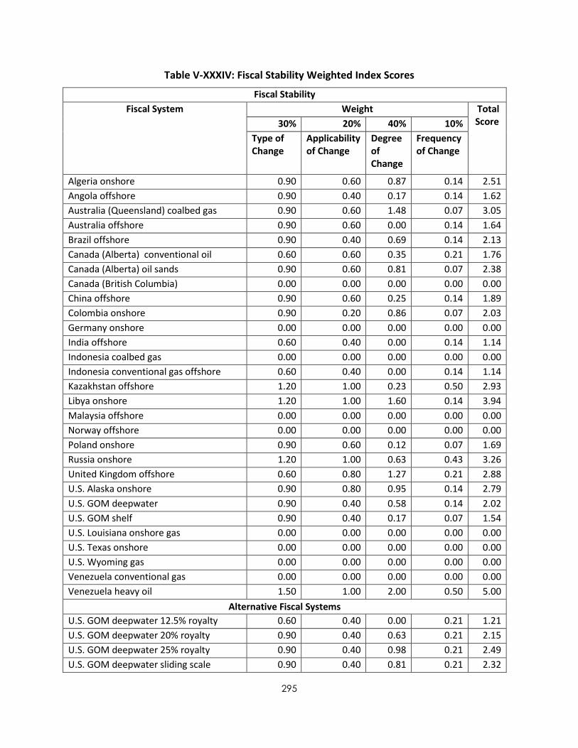
295

Table V-XXXIV: Fiscal Stability Weighted Index Scores

Fiscal Stability


Type of Change


Degree of Change

Frequency of Change

Algeria onshore 0.90 0.60 0.87 0.14 2.51

Angola offshore 0.90 0.40 0.17 0.14 1.62

Australia (Queensland) coalbed gas 0.90 0.60 1.48 0.07 3.05

Australia offshore 0.90 0.60 0.00 0.14 1.64

Brazil offshore 0.90 0.40 0.69 0.14 2.13

Canada (Alberta) conventional oil 0.60 0.60 0.35 0.21 1.76

Canada (Alberta) oil sands 0.90 0.60 0.81 0.07 2.38

Canada (British Columbia) 0.00 0.00 0.00 0.00 0.00

China offshore 0.90 0.60 0.25 0.14 1.89

Colombia onshore 0.90 0.20 0.86 0.07 2.03

Germany onshore 0.00 0.00 0.00 0.00 0.00

India offshore 0.60 0.40 0.00 0.14 1.14

Indonesia coalbed gas 0.00 0.00 0.00 0.00 0.00

Indonesia conventional gas offshore 0.60 0.40 0.00 0.14 1.14

Kazakhstan offshore 1.20 1.00 0.23 0.50 2.93

Libya onshore 1.20 1.00 1.60 0.14 3.94

Malaysia offshore 0.00 0.00 0.00 0.00 0.00

Norway offshore 0.00 0.00 0.00 0.00 0.00

Poland onshore 0.90 0.60 0.12 0.07 1.69

Russia onshore 1.20 1.00 0.63 0.43 3.26

United Kingdom offshore 0.60 0.80 1.27 0.21 2.88

U.S. Alaska onshore 0.90 0.80 0.95 0.14 2.79

U.S. GOM deepwater 0.90 0.40 0.58 0.14 2.02

U.S. GOM shelf 0.90 0.40 0.17 0.07 1.54

U.S. Louisiana onshore gas 0.00 0.00 0.00 0.00 0.00

U.S. Texas onshore 0.00 0.00 0.00 0.00 0.00

U.S. Wyoming gas 0.00 0.00 0.00 0.00 0.00

Venezuela conventional gas 0.00 0.00 0.00 0.00 0.00

Venezuela heavy oil 1.50 1.00 2.00 0.50 5.00


U.S. GOM deepwater 12.5% royalty 0.60 0.40 0.00 0.21 1.21



U.S. GOM deepwater sliding scale 0.90 0.40 0.81 0.21 2.32

296

Fiscal Stability


Type of Change


Degree of Change

Frequency of Change

royalty




U.S. GOM shelf sliding scale royalty 0.90 0.40 0.75 0.14 2.19




U.S. Wyoming gas sliding scale royalty 0.90 0.40 0.29 0.07 1.66

Source: IHS CERA

297

Table V-XXXV: Composite Index—Unweighted Index Scores

Fiscal System Fiscal Terms Revenue Risk

Fiscal Stability

Gov Take

PI IRR Progressivity/Regressivity

Timing of Revenue

Type of Change


Degree of Change

Frequency of Change

Algeria onshore 4.32 0.00 0.43 1.50 1.80 3.00 3.00 2.17 1.43

Angola offshore 3.70 1.93 2.27 0.17 5.00 3.00 2.00 0.43 1.43

Australia (Queensland) coalbed gas 0.89 1.60 2.56 1.67 1.91 3.00 3.00 3.70 0.71

Australia offshore 3.18 0.99 1.50 1.33 2.18 3.00 3.00 0.00 1.43

Brazil offshore 3.28 0.80 2.78 3.67 3.44 3.00 2.00 1.73 1.43

Canada (Alberta) conventional oil 2.49 1.93 2.45 5.00 2.87 2.00 3.00 0.86 2.14

Canada (Alberta) oil sands 2.30 3.46 3.93 3.17 3.04 3.00 3.00 2.01 0.71

Canada (British Columbia) 0.87 2.52 2.97 0.16 0.59 0.00 0.00 0.00 0.00

China offshore 3.88 1.41 3.20 1.33 2.51 3.00 3.00 0.62 1.43

Colombia onshore 4.03 2.40 2.35 0.67 1.85 3.00 1.00 2.16 0.71

Germany onshore 2.46 3.92 4.49 1.83 2.61 0.00 0.00 0.00 0.00

India offshore 2.64 2.43 2.88 2.67 1.86 2.00 2.00 0.00 1.43

Indonesia coalbed gas 3.78 1.81 0.76 2.00 2.15 2.00 2.00 0.00 0.71

Indonesia conventional gas offshore 4.00 2.91 3.38 2.17 0.73 2.00 2.00 0.00 1.43

Kazakhstan offshore 3.73 2.51 2.99 1.50 2.74 4.00 5.00 0.58 5.00

Libya onshore 4.66 1.51 2.09 0.67 2.05 4.00 5.00 4.00 1.43

Malaysia offshore 4.85 3.42 4.27 2.00 1.78 0.00 0.00 0.00 0.00

Norway offshore 3.79 3.02 3.28 4.50 0.00 0.00 0.00 0.00 0.00

Poland onshore 0.00 1.26 2.35 1.33 0.91 3.00 3.00 0.29 0.71

Russia onshore 3.36 2.17 2.78 3.67 3.43 4.00 5.00 1.58 4.29

United Kingdom offshore 2.53 2.66 3.20 0.00 0.28 2.00 4.00 3.17 2.14

U.S. Alaska onshore 3.59 2.81 3.36 3.00 4.79 3.00 4.00 2.37 1.43

U.S. GOM deepwater 2.65 3.01 3.64 3.00 2.71 3.00 2.00 1.44 1.43

U.S. GOM shelf 3.77 4.23 4.83 2.67 2.38 3.00 2.00 0.43 0.71

298


Fiscal Stability

Gov Take

PI IRR Progressivity/Regressivity

Timing of Revenue

Type of Change


Degree of Change

Frequency of Change

U.S. Louisiana onshore gas 4.27 3.05 0.00 1.50 4.39 0.00 0.00 0.00 0.00

U.S. Texas onshore 3.55 3.35 3.42 2.83 4.95 0.00 0.00 0.00 0.00

U.S. Wyoming gas 2.85 2.33 2.73 2.67 3.81 0.00 0.00 0.00 0.00

Venezuela conventional gas 4.18 3.22 3.78 2.17 4.92 0.00 0.00 0.00 0.00

Venezuela heavy oil 5.00 5.00 5.00 0.83 2.90 5.00 5.00 5.00 5.00


U.S. GOM deepwater 12.5% royalty 0.20 0.27 0.33 0.23 0.84 0.12 0.09 0.00 0.06

U.S. GOM deepwater 20% royalty 0.28 0.31 0.37 0.28 0.81 0.18 0.18 0.19 0.06


U.S. GOM deepwater sliding scale royalty 0.28 0.31 0.37 0.12 0.78 0.18 0.18 0.24 0.06

U.S. GOM shelf 12.5% royalty 0.31 0.40 0.46 0.22 0.66 0.12 0.18 0.00 0.04

U.S. GOM shelf 20% royalty 0.39 0.43 0.48 0.28 0.72 0.18 0.18 0.07 0.04


U.S. GOM shelf sliding scale royalty 0.39 0.43 0.49 0.10 0.72 0.18 0.18 0.22 0.04

U.S. Wyoming gas 18.75% royalty 0.32 0.26 0.30 0.27 1.14 0.18 0.18 0.12 0.02

U.S. Wyoming gas 20% royalty 0.33 0.27 0.31 0.25 1.14 0.18 0.18 0.16 0.02


U.S. Wyoming gas sliding scale royalty 0.30 0.24 0.29 0.18 1.08 0.18 0.18 0.09 0.02

Source: IHS CERA

299

Table V-XXXVI: Composite Index—Weighted Score


Fiscal Stability

Weight

40% 30% 30%

Gov Take


Timing of Revenue

Type of Change


Degree of Change

Frequency of Change

Weight

25% 25% 25% 25% 100% 20% 30% 40% 10%

Algeria onshore 0.43 0.00 0.04 0.15 0.54 0.18 0.27 0.26 0.04

Angola offshore 0.37 0.19 0.23 0.02 1.50 0.18 0.18 0.05 0.04

Australia (Queensland) coalbed gas 0.09 0.16 0.26 0.17 0.57 0.18 0.27 0.44 0.02

Australia offshore 0.32 0.10 0.15 0.13 0.65 0.18 0.27 0.00 0.04

Brazil offshore 0.33 0.08 0.28 0.37 1.03 0.18 0.18 0.21 0.04

Canada (Alberta) conventional oil 0.25 0.19 0.25 0.50 0.86 0.12 0.27 0.10 0.06

Canada (Alberta) oil sands 0.23 0.35 0.39 0.32 0.91 0.18 0.27 0.24 0.02

Canada (British Columbia) 0.09 0.25 0.30 0.02 0.18 0.00 0.00 0.00 0.00

China offshore 0.39 0.14 0.32 0.13 0.75 0.18 0.27 0.07 0.04

Colombia onshore 0.40 0.24 0.24 0.07 0.55 0.18 0.09 0.26 0.02

Germany onshore 0.25 0.39 0.45 0.18 0.78 0.00 0.00 0.00 0.00

India offshore 0.26 0.24 0.29 0.27 0.56 0.12 0.18 0.00 0.04

Indonesia coalbed gas 0.38 0.18 0.08 0.20 0.64 0.12 0.18 0.00 0.02

Indonesia conventional gas offshore 0.40 0.29 0.34 0.22 0.22 0.12 0.18 0.00 0.04

Kazakhstan offshore 0.37 0.25 0.30 0.15 0.82 0.24 0.45 0.07 0.15

Libya onshore 0.47 0.15 0.21 0.07 0.61 0.24 0.45 0.48 0.04

Malaysia offshore 0.48 0.34 0.43 0.20 0.53 0.00 0.00 0.00 0.00

Norway offshore 0.38 0.30 0.33 0.45 0.00 0.00 0.00 0.00 0.00

Poland onshore 0.00 0.13 0.24 0.13 0.27 0.18 0.27 0.03 0.02

Russia onshore 0.34 0.22 0.28 0.37 1.03 0.24 0.45 0.19 0.13

United Kingdom offshore 0.25 0.27 0.32 0.00 0.08 0.12 0.36 0.38 0.06

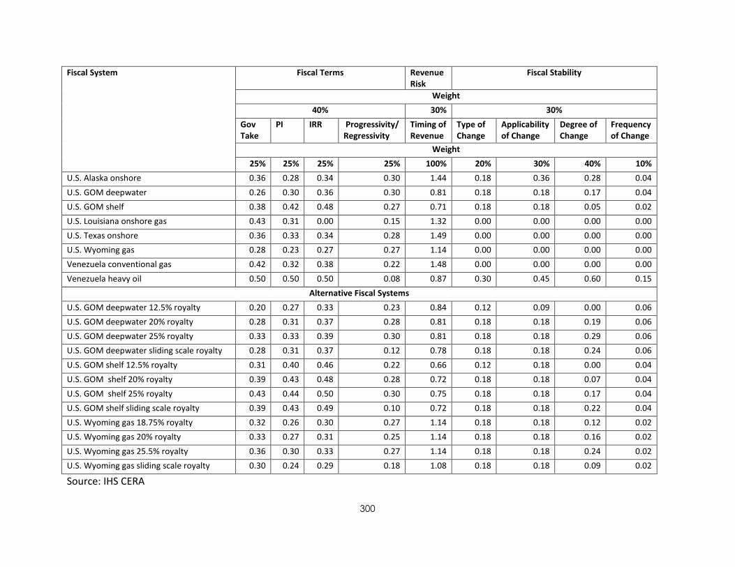
300


Fiscal Stability

Weight

40% 30% 30%

Gov Take


Timing of Revenue

Type of Change


Degree of Change

Frequency of Change

Weight

25% 25% 25% 25% 100% 20% 30% 40% 10%

U.S. Alaska onshore 0.36 0.28 0.34 0.30 1.44 0.18 0.36 0.28 0.04

U.S. GOM deepwater 0.26 0.30 0.36 0.30 0.81 0.18 0.18 0.17 0.04

U.S. GOM shelf 0.38 0.42 0.48 0.27 0.71 0.18 0.18 0.05 0.02

U.S. Louisiana onshore gas 0.43 0.31 0.00 0.15 1.32 0.00 0.00 0.00 0.00

U.S. Texas onshore 0.36 0.33 0.34 0.28 1.49 0.00 0.00 0.00 0.00

U.S. Wyoming gas 0.28 0.23 0.27 0.27 1.14 0.00 0.00 0.00 0.00

Venezuela conventional gas 0.42 0.32 0.38 0.22 1.48 0.00 0.00 0.00 0.00

Venezuela heavy oil 0.50 0.50 0.50 0.08 0.87 0.30 0.45 0.60 0.15


U.S. GOM deepwater 12.5% royalty 0.20 0.27 0.33 0.23 0.84 0.12 0.09 0.00 0.06



U.S. GOM deepwater sliding scale royalty 0.28 0.31 0.37 0.12 0.78 0.18 0.18 0.24 0.06

U.S. GOM shelf 12.5% royalty 0.31 0.40 0.46 0.22 0.66 0.12 0.18 0.00 0.04



U.S. GOM shelf sliding scale royalty 0.39 0.43 0.49 0.10 0.72 0.18 0.18 0.22 0.04


U.S. Wyoming gas 20% royalty 0.33 0.27 0.31 0.25 1.14 0.18 0.18 0.16 0.02


U.S. Wyoming gas sliding scale royalty 0.30 0.24 0.29 0.18 1.08 0.18 0.18 0.09 0.02

Source: IHS CERA

Documents

CERA - BOEM Homepage | BOEM · 2019-10-14 · OCS Study BOEM 2011-xxx IHS CERA Comparative Assessment of the Federal Oil and Gas Fiscal System Final Report Author Irena Agalliu October