Maison des Sciences Économiques, 106-112 boulevard de L'Hôpital, 75647 Paris Cedex 13http://mse.univ-paris1.fr/Publicat.htm

ISSN : 1624-0340

Centre d’Economie de la SorbonneUMR 8174

Public jobs creation and Unemployment dynamics

Céline CHOULET

2006.26

Public jobs creation and Unemployment dynamics∗

Céline Choulet†

Centre d’Economie de la Sorbonne-Université Paris 1

∗Without implication, I would like to give special thanks to Yann Algan, Pierre Cahuc, François Fontaine, GregoryJolivet, Frédéric Karamé, Etienne Lehmann, Claudio Lucifora and Jean-Marc Robin for their helpful comments andsuggestions. I would also like thank the seminar participants at the University Paris 1, at the eea-esem Congress2004, at the eale Conference 2004, at the afse Congress 2004 and at the t2m Conference 2005.

†Centre d’Economie de la Sorbonne, Université Paris 1 Panthéon-Sorbonne, 106-112 Boulevard de l’Hôpital 75647Paris cedex 13. Email: choulet@univ-paris1.fr.

1

Abstract. This paper raises the question of the dynamic effects of public spending in jobs on

labor market performance. We use a dynamic matching model and study how public jobs creation

affects endogenous workers’ decisions to move on the labor market and private-sector firms’ job

creation and destruction decisions. We obtain that it exerts an attracting effect and a fiscal effect

on the labor market that make the unemployment rate and job flows overshoot. As an empirical

illustration, we estimate a svar model that focuses on the consequences of public job creations on

unemployment, wages and job flows dynamics. We confirm our intuition: public employment has

a significant ambiguous effect on private wages.

JEL classification: J45, J21

Keywords: Public sector labor market, Unemployment dynamics

Résumé. Ce papier analyse la dynamique transitoire du marché du travail en présence

d’emplois publics. Un modèle d’appariement dynamique nous permet d’étudier comment les effets

de la création d’emplois publics se propagent dans le temps en présence de deux sources d’éviction:

une concurrence entre les secteurs public et privé pour attirer les travailleurs et une pression fiscale

qui accroît le coût du travail des entreprises privées. L’effet d’attraction et les externalités fiscales

exercées affectent la dynamique du chômage et celle des flux de création et de destruction d’emplois

privés. Un modèle vectoriel auto-régressif, appliqué aux données américaines (1972:2-1993:4), il-

lustre empiriquement notre mécanisme théorique. Nos prédictions théoriques sont confirmées: le

chômage diminue significativement à court terme suite à la création d’emplois publics et l’emploi

public a un effet ambigu significatif sur les salaires privés.

Codes JEL: J45, J21

Mots clés: Emploi public, Dynamique du chômage

2

1 Introduction

The idea that government intervention acts as a stimulus for economic activity in the short run

is popular in traditional Keynesian analysis whereas in the long run, public spending is viewed as

an inefficient policy. In this regard, the question of the dynamic effects of public jobs creation on

labor market performance is relevant. In the short run, public jobs offset the scarcity of private

jobs and reduce unemployment. By offering public infrastructures, the government can exert a

positive externality on the productivity of the private sector, increasing labor demand in that

sector. However, public jobs creation is also expected to crowd-out private employment, as it

increases labor taxes, produces substitutable goods for private ones and exerts wage pressure.

This crowding-out effect can be more than complete, leading to an increase in unemployment.

Thus, in the long run, public job creation can have no significant effect. In this paper, we propose

to study its dynamic effects on unemployment.

Theoretical papers do not have invested the question of the dynamic effects of public jobs

creation on labor market performance. Some empirical papers have do it, linking its negative impact

to an increase in private wage pressure. Edin and Holmlund (1997) use pooled crossed section and

annual time series data for 22 oecd countries over the period 1968-1990. They argue that public

sector employment, in the short run, with wages and prices fixed, decreases unemployment, whereas

there is no significant long run effect (i.e. in the long run, the crowding-out is complete). Some

empirical evidence on dynamic interrelations between aggregate time series on unemployment, real

wages and public employment are provided by Malley and Moutos (1996) for Sweden, Malley and

Moutos (1998) for Japan, Germany and United-States, Demekas and Kontolemis (2000) for Greece.

The crowding-out effect works through a private wage pressure: improvement in employment

outlooks increases workers’ wage demands, and reduces labor demand. Demekas et al. (2000)

estimate a vectorial error correction model (vecm) with Greek data (1971:1-1993:4) on public

employment, unemployment, private and public real wages. In the long run, the crowding-out is

complete and the mean lag (half-life) of the unemployment rate is close to 3 quarters. They use a

static job search model where an increase in public wage, or employment, leads through workers’

moves on the labor market to a higher increase in private sector wage. The unemployment rate

increases as it positively depends on the wage differential between private and public sectors1 .

Malley et al. (1996) estimate a vecmodel with public employment, private employment and capital

stock on Swedish data (1962:3-1990:4). The fall in private employment, due to the increase in public

1We believe this result highly depends on some assumptions. Indeed, we expect, as Holmlund (1997), that thecrowding-out effect should be more than complete when there is a public wage premium, as the attracting effect ofthe public sector increases with the relative level of the public wage.

3

employment, starts after four quarters, with a complete crowding-out effect in five years. In the

long run, the crowding-out is more than complete. Malley et al. (1998) estimate a vectorial auto-

regressive model (var) with public employment, unemployment and private wages on German data

(1960:3-1989:4), on Japan data (1965:4-1994:4) and on us data (1960:3-1996:2). They find that the

crowding-out effect of public employment on private employment is complete, i.e. unemployment

is not affected by changes in government employment. The mean lag is close to 10 years. However,

they argue that this effect doesn’t go through a rise in private real wages.

The empirical evidence of a private wage pressure is not clear. Malley et al. (1998) use a

Choleski decomposition which assumes that unemployment comes before public employment in the

causal order. However, they can’t give any theoretical or empirical support for this assumption.

Demekas et al.’s vecm seems not relevant. First, because they use a job search model with

exogenous probabilities to move on the labor market. Individuals are perfectly insured such as

they have the same utility in and out of the labor market. Second, because the vecm’s results

(irf, fevd) are not discussed. They report a negative correlation between public employment and

private wages, which is not consistent with their theoretical model and not informative for the

response of private wages to innovations in public employment. They obtain that unemployment

is positively correlated with the wage differential but they do not test formally for the positive

impact of an increase in the wage differential on unemployment. Malley et al. (1996) do not

include wages in their vecm. Therefore, we can not conclude on the empirical relevance of private

wages as propagation channel of public jobs creation. Malley et al. (1998) attribute the fall in

private employment to taxes and fixed costs that increase disincentives for private-sector firm and

job creation. However, they don’t evaluate the relevance of such a propagation channel.

It seems that the wage channel is at best a theoretical possibility for which there is no convinc-

ing evidence. The result of a private wage pressure is obtained in bargaining models (Holmlund,

1997, Algan, Cahuc and Zylberberg, 2002) or job search models (Demekas et al., 2000), in which

the improvement of employment outlooks increases workers’ wage demands. However, fiscal impli-

cations of public jobs creation have to be taken into account. If firms can shift all the tax burden

onto workers, private wages can decline. If there is no complete shifting, we expect changes in

firms’ job creation and destruction decisions. Demand studies only find very partial shifting of

taxes onto workers (in the form of lower wage rates) and a higher, but not complete, shifting onto

labor demand (with time-series data) (Hamermesh, 1993). We believe payroll taxes are a relevant

propagation channel of the public crowding-out effect on private labor demand. We propose a

theoretical model and a var estimation, in which we include private job creation and destruction

4

rates to reflect fiscal distortive effect of public jobs creation and to offset the traditional wage

pressure result.

The paper is organized as follows. In Sections 2 and 3, we propose a theoretical mechanism.

We use a dynamic matching model. This model permits to study the propagation mechanism of

the public shock on the labor market. With endogenous job creation and destruction decisions, the

asymmetries that characterize unemployment dynamics are taken into account. Instantaneously,

newly created public jobs are filled by the unemployed workers searching for a public job. Thus, in

the short run, the unemployment rate decreases and the public sector exerts an attracting effect

on private workers. Due to its fiscal implications, public jobs creation affects the private-sector job

creation and destruction decisions. The disincentives for private jobs creation that distortive labor

taxes generate make the unemployment rate increase. In the long run, the net impact depends on

the size of the public wage premium. In Section 4, we empirically invest the question of the dynamic

effects of public job creation on the unemployment, private wages, job creation and destruction

rates. We use a structural vectorial auto-regressive (svar) technique on us data in order to

illustrate our model. The data were obtained from the oecd Employment Outlooks, lrd and

cps database. The data cover the period 1972:2-1993:4. We use short-run restrictions (Blanchard,

1989, Davis and Haltiwanger, 1992, Karamé and Mioubi, 1998). We obtain a significant short run

fall in the unemployment rate, followed by an overshooting. Labor market flows dynamics are

consistent with our matching model. We also obtain that increases in public employment rate are

partly due to innovations in unemployment, suggesting a government response to unemployment.

Public shock highly affects private wages but the net impact is not clear. Section 5 concludes.

2 A dynamic matching model with public jobs

We consider a dynamic matching model of the labor market with public and private jobs. Our

model features three types of agents: private- and public- sectors workers, firms and the govern-

ment. The size of the labor force is constant and normalized to one. All individuals have the same

preferences, live infinite lives and are risk-neutral. There is a common discount rate denoted by r.

We consider a framework in which unemployed workers can search either for a public job or for a

private job, but not for both types of job at the same time. This assumption is convenient with the

fact that, in many oecd countries, the public sector has a specific hiring process, which requires

specific knowledge and/or networks. Unemployed workers can move between sectors. They search

in the sector in which the return of search is the highest. In equilibrium, there is an arbitrage

5

condition, which implies that the return of search is the same in both sectors. For the sake of

simplicity, job to job mobility is not taken into account. There are lg jobs in the public sector and

lp jobs in the private sector. Accordingly, the number of unemployed workers is: u = 1− lp − lg.

2.1 Technologies

In the private sector, each firm has one job. When the job is filled, it produces a numeraire output,

using labor. All new jobs are created at maximum productivity2. We note px the productivity of a

private job where p is a general productivity parameter and x an idiosyncratic one. p is a positive

constant parameter. When a shock arrives, the idiosyncratic productivity is drawn from a general

distribution F (x), with 0 ≤ x ≤ eu. This productivity is independent of initial productivity and

irreversible. Idiosyncratic shocks arrive to jobs at Poisson rate qp. Note Jp(x) the value of a filled

job with idiosyncratic productivity x. At some of the idiosyncratic productivities that firms face,

production is profitable, but at some others it is not. When a shock arrives, it can be shown that

the optimal decision for the firm is to continue production at the new productivity if Jp(x) ≥ 0but to destroy the job if Jp(x) < 0. As Jp(x) is a monotone continuous increasing function of x,

the job destruction rule Jp(x) < 0 satisfies the reservation property with respect to the reservation

productivity R, defined by Jp(R) = 0. By the reservation property, firms destroy all jobs with

idiosyncratic productivity x ≤ R and continue producing in all jobs with productivity x > R3 .

In the public sector, each job produces one unit of public goods, which are consumed by all

individuals. Public goods provide v(lg) utility. This utility is increasing at a decreasing rate in

the amount of the public good, i.e. v0(lg) > 0 and v00(lg) < 0. The public-sector employment and

wage levels are exogenous. Public jobs are destroyed at rate qg.

2.2 Matching function

Our model borrows from Mortensen and Pissarides (1994). In the private sector, hiring a worker

and searching for a job are costly activities. Private vacant jobs and unemployed workers are

brought together in pairs through an imperfect matching process. We assume a matching function

that gives the number of jobs formed, at any moment in time, as a function of the number of

workers looking for jobs and the number of firms looking for workers. A job can be filled or vacant,

but only vacant jobs search for workers. Similarly, a worker can be employed or unemployed, but

only unemployed workers search for jobs.

2Newly-created jobs are assumed more productive than existing ones, as they benefit from the best technologyin the market. We would obtain the same qualitative results with a stochastic matching model.

3Using a minimum required idiosyncratic productivity explains why firms shut down rather than make marginalchanges that would allow them to continue in existence.

6

Let up denote the number of unemployed workers who look for a private job and vp the number

of vacancies in the private sector. The number of employer-worker contacts per unit of time is given

by m (up, vp). The matching function is twice continuously differentiable, increasing and concave

in both of its arguments, and linearly homogeneous. Linear homogeneity of the matching function

allows to express the per period probability for a private vacant job (unemployed worker) to meet

an unemployed worker (a vacant job) as a function of the labor market tightness ratio, θ = vp/up.

A vacant job can meet on average m (up, vp) /vp = m (θ) unemployed workers per period, with

m0 (·) < 0. Similarly, the rate at which unemployed job seekers can meet private jobs at each

date is θm (θ), an increasing function of θ. Since private jobs are destroyed at rate qpF (R), the

evolution of mean private-sector unemployment is given by the difference between the two flows:

up = qpF (R)lp − θm(θ)up. (1)

In the public sector, the government recruits employees at random among the ug unemployed

workers who look for a public job. The evolution of public-sector unemployment is therefore given

by:

ug = qglg − gug. (2)

So, the evolution of total unemployment reads:

u = qpF (R)lp + qglg − θm(θ)up − gug. (3)

2.3 Expected asset values

Expected profit from a filled job and from a vacant job

Using the discount rate r, the present-discounted value of expected profit from an occupied job,

with productivity in the range R ≤ x ≤ eu, satisfies:

rJp(x) = px− wp(x)(1 + τ) + qp

Z eu

R

Jp(s)dF (s) + qpF (R)Vp − qpJ

p(x) + Jp(x), (4)

where wp(x) is the wage rate, which is determined by a bargain between the firm and the worker

for all R < x ≤ eu. Wages are taxed at the distortive rate τ . Whenever an idiosyncratic shock

arrives, the firm continues producing for a new value Jp(s) if the new idiosyncratic productivity

is in the range R < s ≤ eu, or destroys the job for an expected return V p otherwise. Jp is the

expected capital gain from changes in job value during adjustment.

V p is the present-discounted value of expected profit from a vacant job and it is given by:

rV p = −h+m(θ) [Jp(eu)− V p] + V p,

7

with h the hiring cost. In our simulations, this cost will be made proportional to the mean

productivity, as it is assumed that it is more costly to hire more productive workers.

We assume that all profit opportunities from new jobs are exploited in the steady state and

out of it, driving rents from vacant jobs to zero V p = V p = 0, which implies:

Jp(eu) =h

m(θ)

This condition states that in equilibrium, private-sector labor market tightness is such that the

expected profit from a new job is equal to the expected cost of hiring a worker.

Expected utilities of workers

We have neglected labor intensity and search costs. A private- or public-sector worker instan-

taneously enjoys the utility from his wage rate, wp(x) or wg, and from public goods, v(lg). The

unemployed workers enjoy unemployment benefits, z, and public goods, v(lg)4 . Let W pe (x), W

ge ,

W pu and W g

u denote, respectively, the expected present values of the lifetime utility for privately

employed, publicly employed or unemployed workers.

In the private sector, the returns from working at a job with idiosyncratic productivity x ]R, eu]

satisfy:

rW pe (x) = wp(x) + v(lg) + qp

Z eu

R

W pe (s)dF (s) + qpF (R)W

pu − qpW

pe (x) + W p

e (x), (5)

rW pu = z + v(lg) + θm(θ) [W p

e (eu)−W pu ] + W p

u , (6)

rW ge = wg + v(lg) + qg [W

gu −W g

e ] + W ge ,

rW gu = z + v(lg) + g [W g

e −W gu ] + W p

u . (7)

Whenever a shock arrives, the private-sector worker remains employed for new returns W pe (s) if

the new idiosyncratic productivity is in the range R < s ≤ eu, or becomes unemployed for an

expected return W pu otherwise.

4Considering exogenous unemployment benefits permit to obtain a partial shifting of the tax burden onto workers.With unemployment benefits index-linked on current private wages, firms would shift all the tax burden onto workers,through lower wages. However, note that the unemployment dynamics would be the same as with exogenous benefits.

8

2.4 Steady-state equilibrium

In the steady-state, the mean rate of unemployment is constant, u = 0. Its steady-state value is:

u =qpF (R)

θm(θ)lp +

qgglg. (8)

Therefore, in equilibrium, the mean number of workers who go on unemployment qpF (R)lp+qglg is

equal to the mean number of workers who get out of unemployment θm(θ)up+gug. In the steady-

state, the expected capital gains, during adjustment, from changes in jobs value or in utilities are

null, Jp(x) = W pe (x) = W p

u = W pu = W p

u = 0.

Sharing rule

The private wage rate derived from the Nash bargaining solution is the one that maximizes the

weighted product of the worker’s and the firm’s net return from the job match S(x) = W pe (x) −

W pu + Jp(x) − V p. It satisfies wp(x) = argmax (W p

e (x)−W pu )

γ (Jp(x)− V p)1−γ , with γ ∈ [0, 1]the relative measure of labor’s bargaining strength. The first-order maximization condition gives

the sharing rule:

W pe (x)−W p

u =γ

γ + (1− γ)(1 + τ)(W p

e (x)−W pu + Jp(x)), (9)

where γ/[γ + (1− γ)(1 + τ)] is the worker’s share in total surplus, which decreases with a rise in

the tax rate.

By substituting W pe (x), W

pu and Jp(x) from (5), (6) and (4) into (9), one gets:

wp(x) = (1− γ)z +γ

1 + τ(px+ hθ), (10)

with x ]R, eu].

So, the mean expected wage rate of a private employed worker reads:

E (wp(x)/x > R) = (1− γ)z +γ

1 + τ(pE (x/x > R) + hθ).

with E (x/x > R) =

·³qpF (R)

qplp

´eu+

³qp(1−F (R))

qplp

´Z eu

R

x dF (x)1−F (R)

¸/lp the mean idiosyncratic

productivity. We note wp the mean wage rate. This wage is renegociated when a new information

arrives.

Private-sector job creation and destruction conditions

Substitution of the wage equation (10) into (4) gives

(r + qp)Jp(x) = (1− γ)(px− z(1 + τ))− γhθ + qp

Z eu

R

Jp(s)dF (s). (11)

9

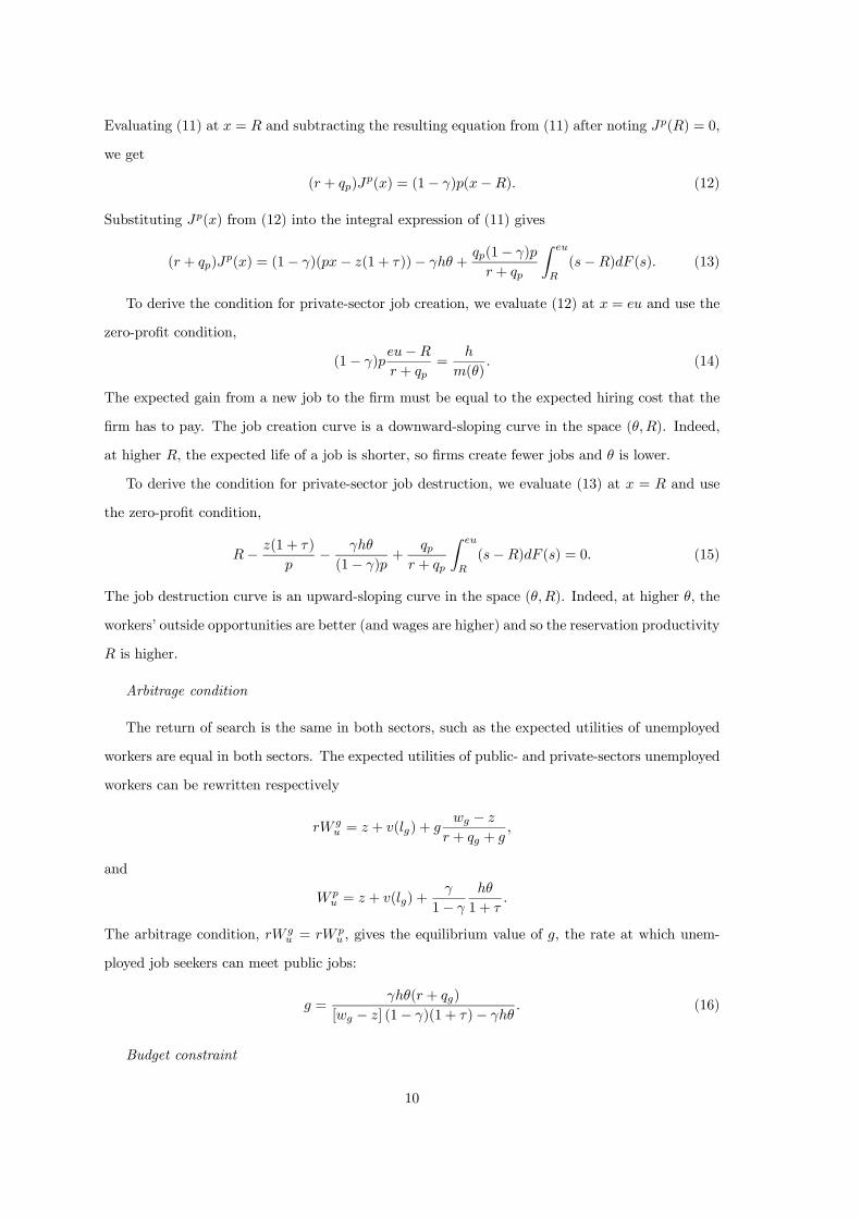
Evaluating (11) at x = R and subtracting the resulting equation from (11) after noting Jp(R) = 0,

we get

(r + qp)Jp(x) = (1− γ)p(x−R). (12)

Substituting Jp(x) from (12) into the integral expression of (11) gives

(r + qp)Jp(x) = (1− γ)(px− z(1 + τ))− γhθ +

qp(1− γ)p

r + qp

Z eu

R

(s−R)dF (s). (13)

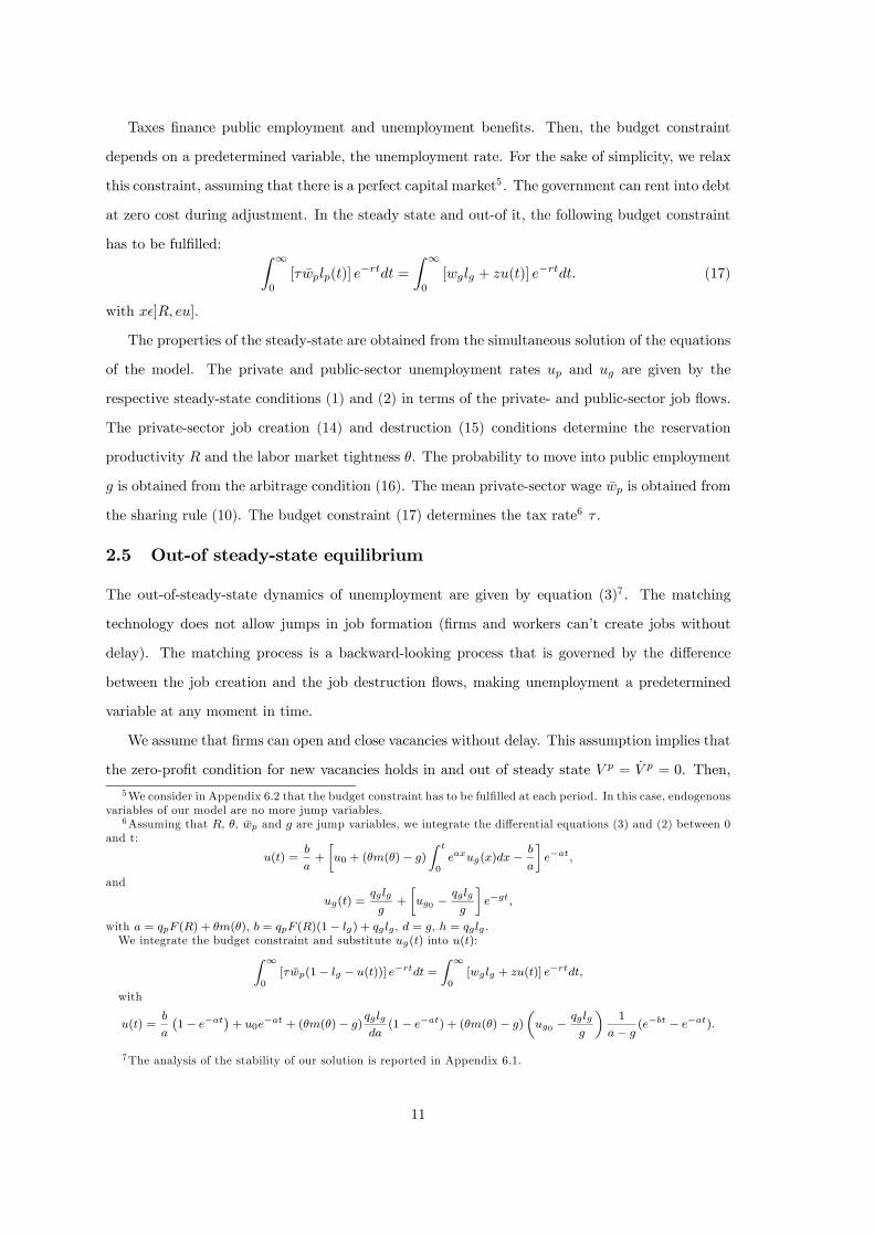
To derive the condition for private-sector job creation, we evaluate (12) at x = eu and use the

zero-profit condition,

(1− γ)peu−R

r + qp=

h

m(θ). (14)

The expected gain from a new job to the firm must be equal to the expected hiring cost that the

firm has to pay. The job creation curve is a downward-sloping curve in the space (θ,R). Indeed,

at higher R, the expected life of a job is shorter, so firms create fewer jobs and θ is lower.

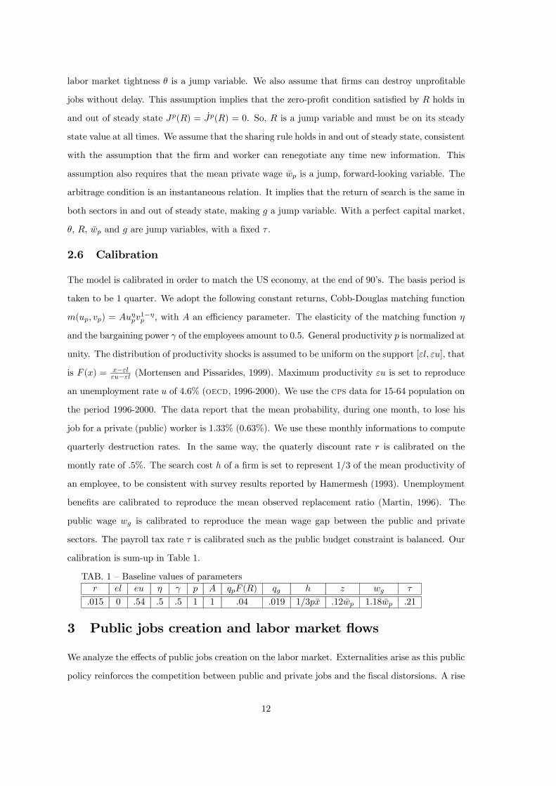
To derive the condition for private-sector job destruction, we evaluate (13) at x = R and use

the zero-profit condition,

R− z(1 + τ)

p− γhθ

(1− γ)p+

qpr + qp

Z eu

R

(s−R)dF (s) = 0. (15)

The job destruction curve is an upward-sloping curve in the space (θ,R). Indeed, at higher θ, the

workers’ outside opportunities are better (and wages are higher) and so the reservation productivity

R is higher.

Arbitrage condition

The return of search is the same in both sectors, such as the expected utilities of unemployed

workers are equal in both sectors. The expected utilities of public- and private-sectors unemployed

workers can be rewritten respectively

rW gu = z + v(lg) + g

wg − z

r + qg + g,

and

W pu = z + v(lg) +

γ

1− γ

hθ

1 + τ.

The arbitrage condition, rW gu = rW p

u , gives the equilibrium value of g, the rate at which unem-

ployed job seekers can meet public jobs:

g =γhθ(r + qg)

[wg − z] (1− γ)(1 + τ)− γhθ. (16)

Budget constraint

10

Taxes finance public employment and unemployment benefits. Then, the budget constraint

depends on a predetermined variable, the unemployment rate. For the sake of simplicity, we relax

this constraint, assuming that there is a perfect capital market5. The government can rent into debt

at zero cost during adjustment. In the steady state and out-of it, the following budget constraint

has to be fulfilled: Z ∞0

[τwplp(t)] e−rtdt =

Z ∞0

[wglg + zu(t)] e−rtdt. (17)

with x ]R, eu].

The properties of the steady-state are obtained from the simultaneous solution of the equations

of the model. The private and public-sector unemployment rates up and ug are given by the

respective steady-state conditions (1) and (2) in terms of the private- and public-sector job flows.

The private-sector job creation (14) and destruction (15) conditions determine the reservation

productivity R and the labor market tightness θ. The probability to move into public employment

g is obtained from the arbitrage condition (16). The mean private-sector wage wp is obtained from

the sharing rule (10). The budget constraint (17) determines the tax rate6 τ .

2.5 Out-of steady-state equilibrium

The out-of-steady-state dynamics of unemployment are given by equation (3)7. The matching

technology does not allow jumps in job formation (firms and workers can’t create jobs without

delay). The matching process is a backward-looking process that is governed by the difference

between the job creation and the job destruction flows, making unemployment a predetermined

variable at any moment in time.

We assume that firms can open and close vacancies without delay. This assumption implies that

the zero-profit condition for new vacancies holds in and out of steady state V p = V p = 0. Then,

5We consider in Appendix 6.2 that the budget constraint has to be fulfilled at each period. In this case, endogenousvariables of our model are no more jump variables.

6Assuming that R, θ, wp and g are jump variables, we integrate the differential equations (3) and (2) between 0and t:

u(t) =b

a+ u0 + (θm(θ)− g)

t

0eaxug(x)dx− b

ae−at,

and

ug(t) =qglg

g+ ug0 −

qglg

ge−gt,

with a = qpF (R) + θm(θ), b = qpF (R)(1− lg) + qglg , d = g, h = qglg .We integrate the budget constraint and substitute ug(t) into u(t):

∞

0[τwp(1− lg − u(t))] e−rtdt =

∞

0[wglg + zu(t)] e−rtdt,

with

u(t) =b

a1− e−at + u0e

−at + (θm(θ)− g)qglg

da(1− e−at) + (θm(θ)− g) ug0 −

qglg

g

1

a− g(e−bt − e−at).

7The analysis of the stability of our solution is reported in Appendix 6.1.

11

labor market tightness θ is a jump variable. We also assume that firms can destroy unprofitable

jobs without delay. This assumption implies that the zero-profit condition satisfied by R holds in

and out of steady state Jp(R) = Jp(R) = 0. So, R is a jump variable and must be on its steady

state value at all times. We assume that the sharing rule holds in and out of steady state, consistent

with the assumption that the firm and worker can renegotiate any time new information. This

assumption also requires that the mean private wage wp is a jump, forward-looking variable. The

arbitrage condition is an instantaneous relation. It implies that the return of search is the same in

both sectors in and out of steady state, making g a jump variable. With a perfect capital market,

θ, R, wp and g are jump variables, with a fixed τ .

2.6 Calibration

The model is calibrated in order to match the US economy, at the end of 90’s. The basis period is

taken to be 1 quarter. We adopt the following constant returns, Cobb-Douglas matching function

m(up, vp) = Auηpv1−ηp , with A an efficiency parameter. The elasticity of the matching function η

and the bargaining power γ of the employees amount to 0.5. General productivity p is normalized at

unity. The distribution of productivity shocks is assumed to be uniform on the support [εl, εu], that

is F (x) = x−εlεu−εl (Mortensen and Pissarides, 1999). Maximum productivity εu is set to reproduce

an unemployment rate u of 4.6% (oecd, 1996-2000). We use the cps data for 15-64 population on

the period 1996-2000. The data report that the mean probability, during one month, to lose his

job for a private (public) worker is 1.33% (0.63%). We use these monthly informations to compute

quarterly destruction rates. In the same way, the quaterly discount rate r is calibrated on the

montly rate of .5%. The search cost h of a firm is set to represent 1/3 of the mean productivity of

an employee, to be consistent with survey results reported by Hamermesh (1993). Unemployment

benefits are calibrated to reproduce the mean observed replacement ratio (Martin, 1996). The

public wage wg is calibrated to reproduce the mean wage gap between the public and private

sectors. The payroll tax rate τ is calibrated such as the public budget constraint is balanced. Our

calibration is sum-up in Table 1.

TAB. 1 — Baseline values of parametersr el eu η γ p A qpF (R) qg h z wg τ

.015 0 .54 .5 .5 1 1 .04 .019 1/3px .12wp 1.18wp .21

3 Public jobs creation and labor market flows

We analyze the effects of public jobs creation on the labor market. Externalities arise as this public

policy reinforces the competition between public and private jobs and the fiscal distorsions. A rise

12

in public employment increases the public share of the labor force and decreases the private share.

Out-of steady state, unemployment decreases in the short term.

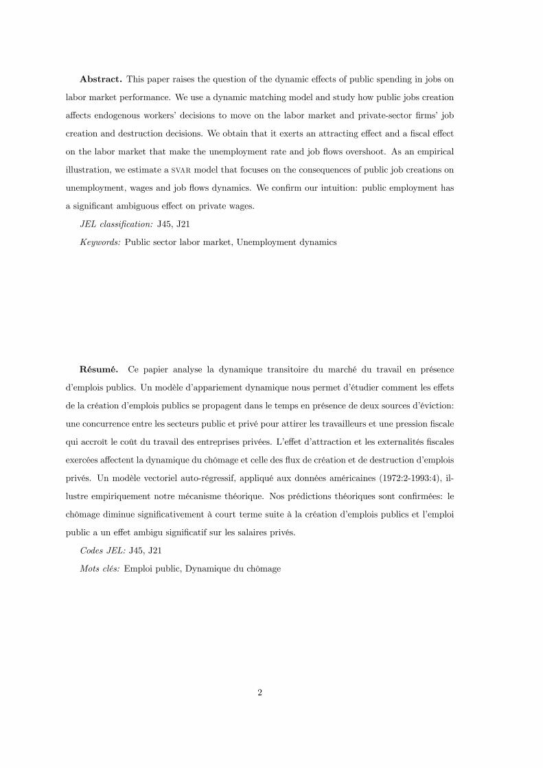
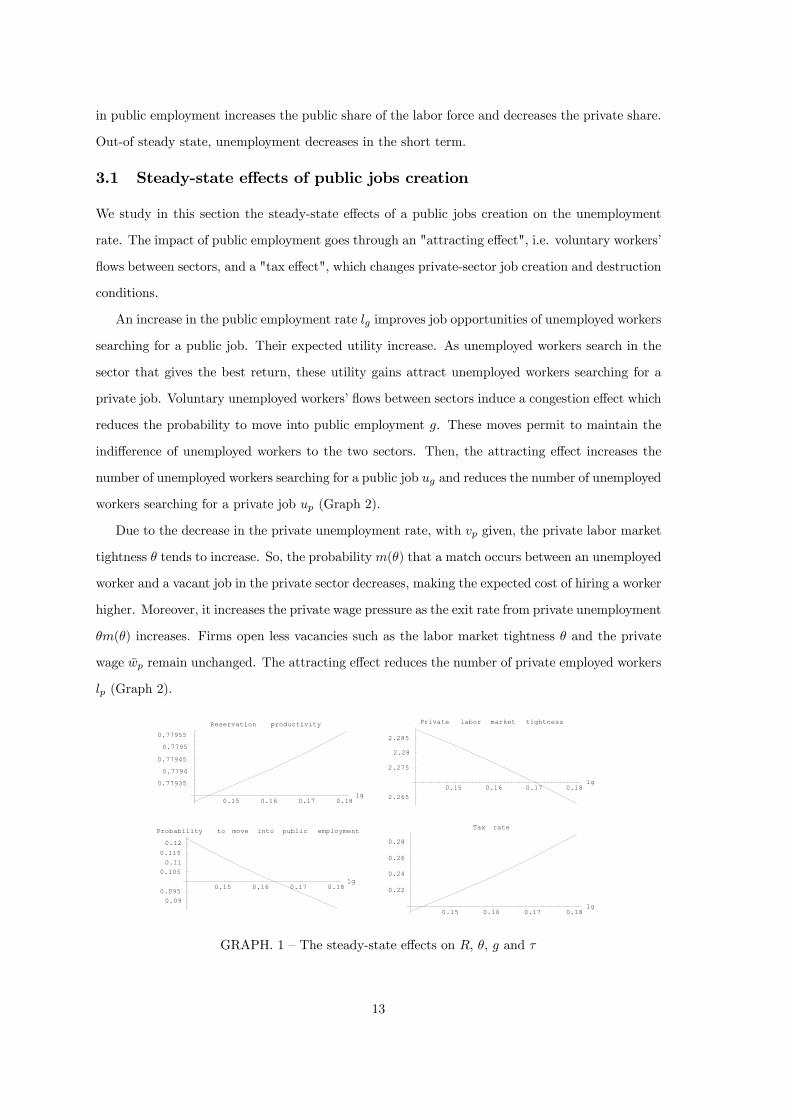
3.1 Steady-state effects of public jobs creation

We study in this section the steady-state effects of a public jobs creation on the unemployment

rate. The impact of public employment goes through an "attracting effect", i.e. voluntary workers’

flows between sectors, and a "tax effect", which changes private-sector job creation and destruction

conditions.

An increase in the public employment rate lg improves job opportunities of unemployed workers

searching for a public job. Their expected utility increase. As unemployed workers search in the

sector that gives the best return, these utility gains attract unemployed workers searching for a

private job. Voluntary unemployed workers’ flows between sectors induce a congestion effect which

reduces the probability to move into public employment g. These moves permit to maintain the

indifference of unemployed workers to the two sectors. Then, the attracting effect increases the

number of unemployed workers searching for a public job ug and reduces the number of unemployed

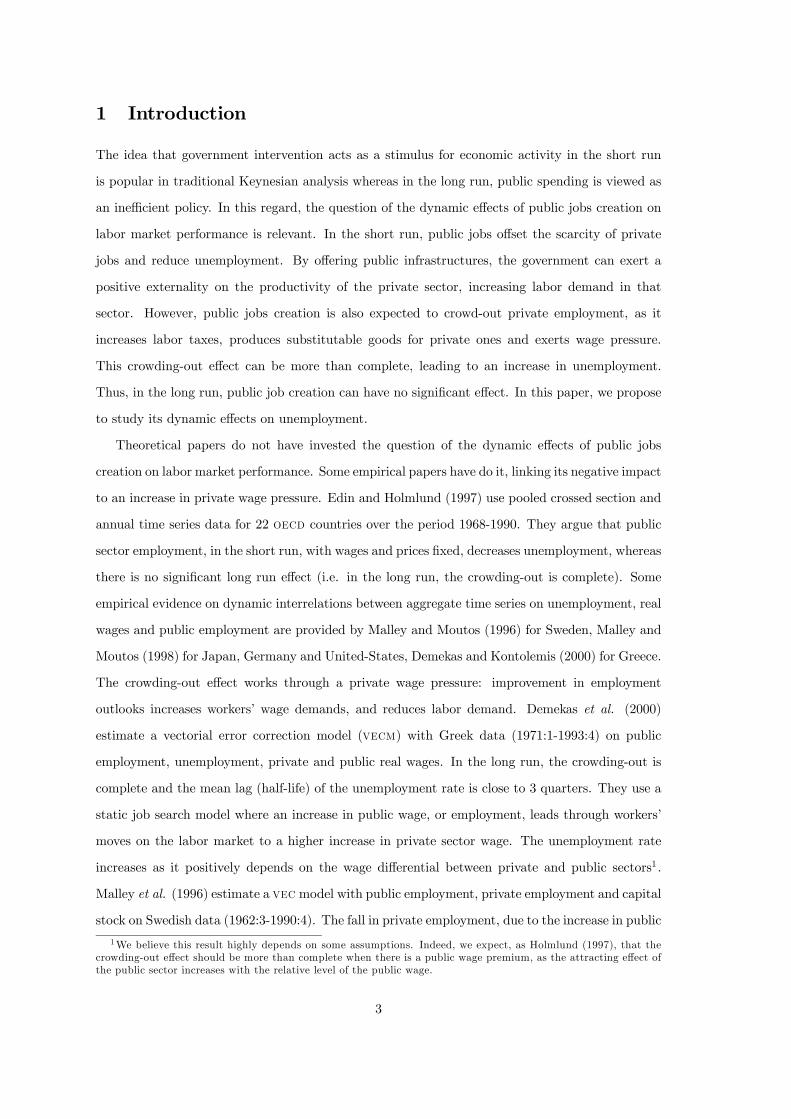
workers searching for a private job up (Graph 2).

Due to the decrease in the private unemployment rate, with vp given, the private labor market

tightness θ tends to increase. So, the probabilitym(θ) that a match occurs between an unemployed

worker and a vacant job in the private sector decreases, making the expected cost of hiring a worker

higher. Moreover, it increases the private wage pressure as the exit rate from private unemployment

θm(θ) increases. Firms open less vacancies such as the labor market tightness θ and the private

wage wp remain unchanged. The attracting effect reduces the number of private employed workers

lp (Graph 2).

0.15 0.16 0.17 0.18lg

0.090.095

0.1050.11

0.115

0.12

Probability to move into public employment

0.15 0.16 0.17 0.18lg

0.22

0.24

0.26

0.28

Tax rate

0.15 0.16 0.17 0.18lg

0.77935

0.7794

0.77945

0.7795

0.77955

Reservation productivity

0.15 0.16 0.17 0.18lg

2.265

2.275

2.28

2.285

Private labor market tightness

GRAPH. 1 — The steady-state effects on R, θ, g and τ

13

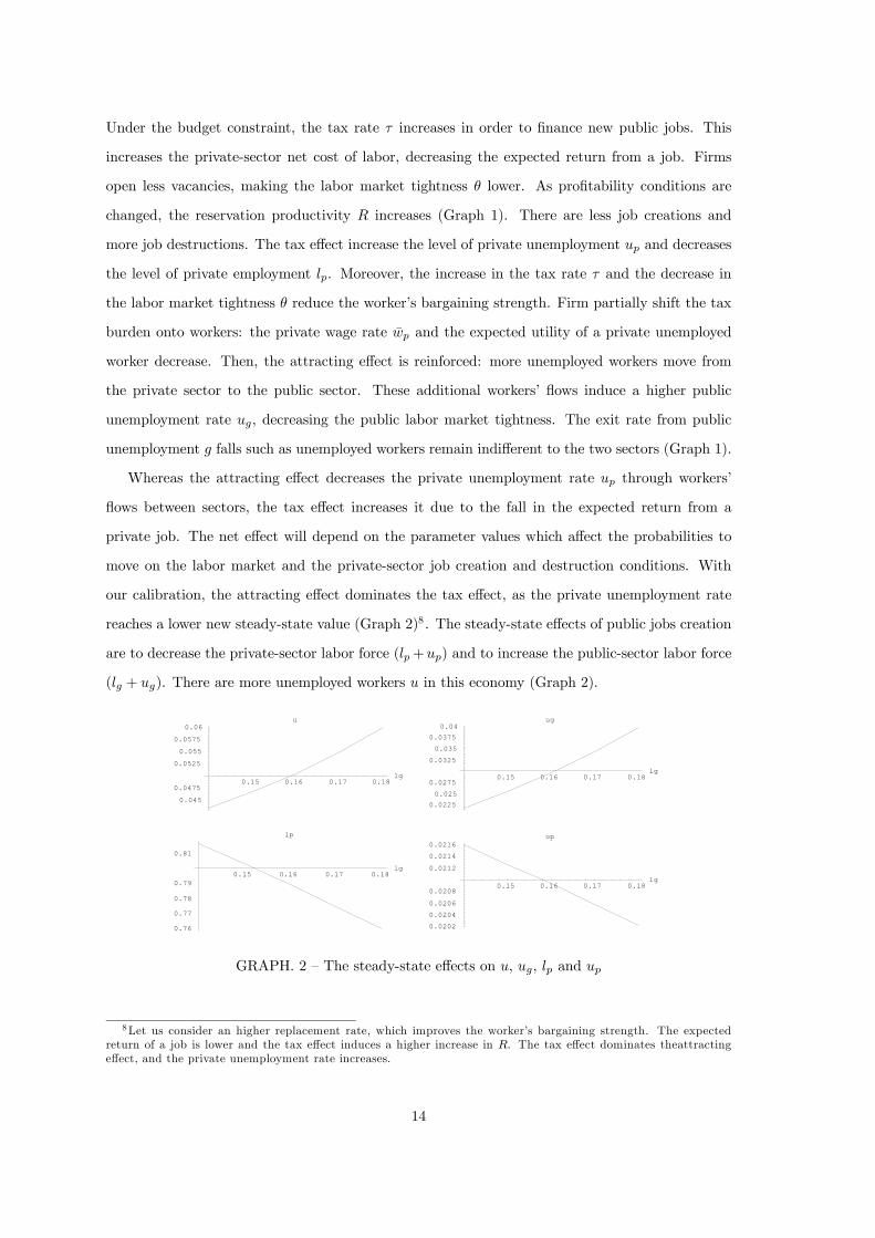
Under the budget constraint, the tax rate τ increases in order to finance new public jobs. This

increases the private-sector net cost of labor, decreasing the expected return from a job. Firms

open less vacancies, making the labor market tightness θ lower. As profitability conditions are

changed, the reservation productivity R increases (Graph 1). There are less job creations and

more job destructions. The tax effect increase the level of private unemployment up and decreases

the level of private employment lp. Moreover, the increase in the tax rate τ and the decrease in

the labor market tightness θ reduce the worker’s bargaining strength. Firm partially shift the tax

burden onto workers: the private wage rate wp and the expected utility of a private unemployed

worker decrease. Then, the attracting effect is reinforced: more unemployed workers move from

the private sector to the public sector. These additional workers’ flows induce a higher public

unemployment rate ug, decreasing the public labor market tightness. The exit rate from public

unemployment g falls such as unemployed workers remain indifferent to the two sectors (Graph 1).

Whereas the attracting effect decreases the private unemployment rate up through workers’

flows between sectors, the tax effect increases it due to the fall in the expected return from a

private job. The net effect will depend on the parameter values which affect the probabilities to

move on the labor market and the private-sector job creation and destruction conditions. With

our calibration, the attracting effect dominates the tax effect, as the private unemployment rate

reaches a lower new steady-state value (Graph 2)8. The steady-state effects of public jobs creation

are to decrease the private-sector labor force (lp+up) and to increase the public-sector labor force

(lg + ug). There are more unemployed workers u in this economy (Graph 2).

0.15 0.16 0.17 0.18lg

0.76

0.77

0.78

0.79

0.81

lp

0.15 0.16 0.17 0.18lg

0.0202

0.0204

0.0206

0.0208

0.0212

0.0214

0.0216up

0.15 0.16 0.17 0.18lg

0.045

0.0475

0.0525

0.055

0.0575

0.06u

0.15 0.16 0.17 0.18lg

0.0225

0.025

0.0275

0.0325

0.035

0.0375

0.04ug

GRAPH. 2 — The steady-state effects on u, ug, lp and up

8Let us consider an higher replacement rate, which improves the worker’s bargaining strength. The expectedreturn of a job is lower and the tax effect induces a higher increase in R. The tax effect dominates theattractingeffect, and the private unemployment rate increases.

14

3.2 Out-of Steady-State Dynamics

We analyze, in this section, the out of steady-state dynamics of the unemployment rate.

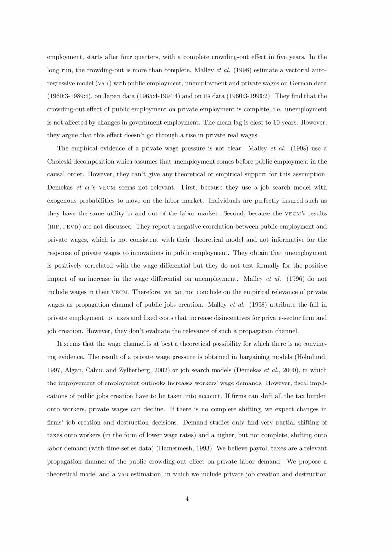
Instantaneously

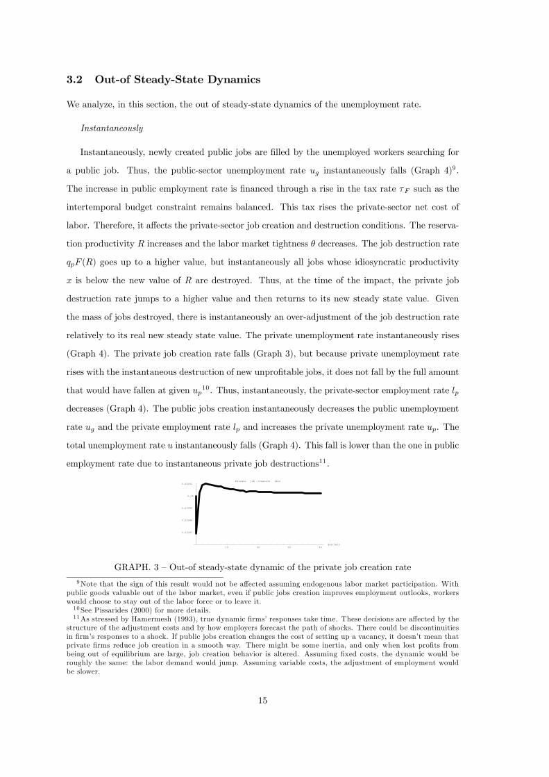
Instantaneously, newly created public jobs are filled by the unemployed workers searching for

a public job. Thus, the public-sector unemployment rate ug instantaneously falls (Graph 4)9.

The increase in public employment rate is financed through a rise in the tax rate τF such as the

intertemporal budget constraint remains balanced. This tax rises the private-sector net cost of

labor. Therefore, it affects the private-sector job creation and destruction conditions. The reserva-

tion productivity R increases and the labor market tightness θ decreases. The job destruction rate

qpF (R) goes up to a higher value, but instantaneously all jobs whose idiosyncratic productivity

x is below the new value of R are destroyed. Thus, at the time of the impact, the private job

destruction rate jumps to a higher value and then returns to its new steady state value. Given

the mass of jobs destroyed, there is instantaneously an over-adjustment of the job destruction rate

relatively to its real new steady state value. The private unemployment rate instantaneously rises

(Graph 4). The private job creation rate falls (Graph 3), but because private unemployment rate

rises with the instantaneous destruction of new unprofitable jobs, it does not fall by the full amount

that would have fallen at given up10. Thus, instantaneously, the private-sector employment rate lp

decreases (Graph 4). The public jobs creation instantaneously decreases the public unemployment

rate ug and the private employment rate lp and increases the private unemployment rate up. The

total unemployment rate u instantaneously falls (Graph 4). This fall is lower than the one in public

employment rate due to instantaneous private job destructions11 .

10 20 30 40quarters

0.03997

0.03998

0.03999

0.04

0.04001Private job creation rate

GRAPH. 3 — Out-of steady-state dynamic of the private job creation rate

9Note that the sign of this result would not be affected assuming endogenous labor market participation. Withpublic goods valuable out of the labor market, even if public jobs creation improves employment outlooks, workerswould choose to stay out of the labor force or to leave it.10 See Pissarides (2000) for more details.11As stressed by Hamermesh (1993), true dynamic firms’ responses take time. These decisions are affected by the

structure of the adjustment costs and by how employers forecast the path of shocks. There could be discontinuitiesin firm’s responses to a shock. If public jobs creation changes the cost of setting up a vacancy, it doesn’t mean thatprivate firms reduce job creation in a smooth way. There might be some inertia, and only when lost profits frombeing out of equilibrium are large, job creation behavior is altered. Assuming fixed costs, the dynamic would beroughly the same: the labor demand would jump. Assuming variable costs, the adjustment of employment wouldbe slower.

15

16

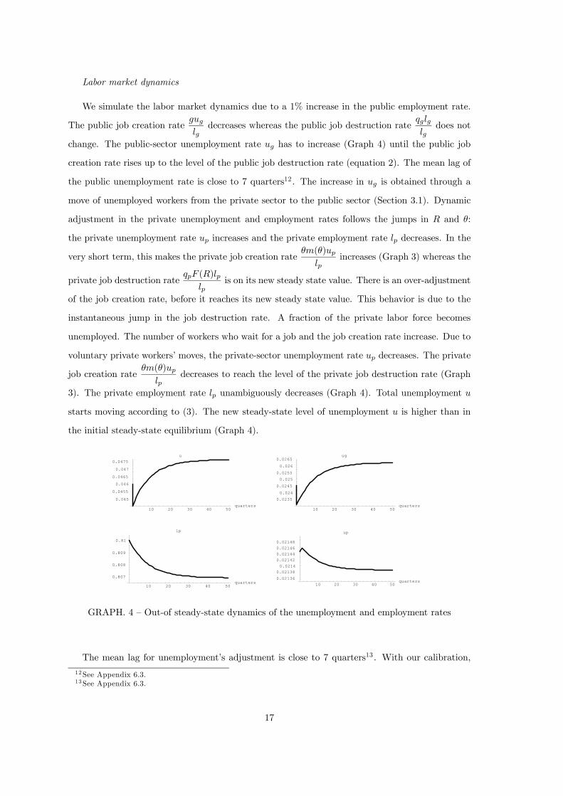
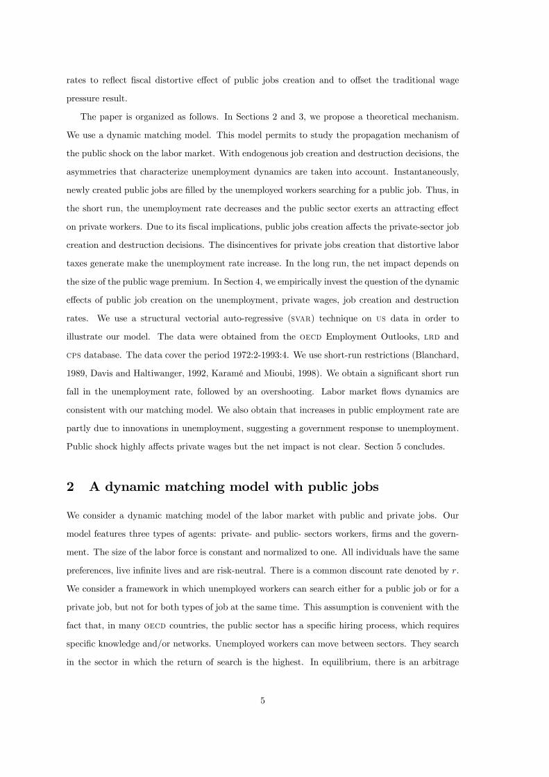
Labor market dynamics

We simulate the labor market dynamics due to a 1% increase in the public employment rate.

The public job creation rateguglg

decreases whereas the public job destruction rateqglglg

does not

change. The public-sector unemployment rate ug has to increase (Graph 4) until the public job

creation rate rises up to the level of the public job destruction rate (equation 2). The mean lag of

the public unemployment rate is close to 7 quarters12. The increase in ug is obtained through a

move of unemployed workers from the private sector to the public sector (Section 3.1). Dynamic

adjustment in the private unemployment and employment rates follows the jumps in R and θ:

the private unemployment rate up increases and the private employment rate lp decreases. In the

very short term, this makes the private job creation rateθm(θ)up

lpincreases (Graph 3) whereas the

private job destruction rateqpF (R)lp

lpis on its new steady state value. There is an over-adjustment

of the job creation rate, before it reaches its new steady state value. This behavior is due to the

instantaneous jump in the job destruction rate. A fraction of the private labor force becomes

unemployed. The number of workers who wait for a job and the job creation rate increase. Due to

voluntary private workers’ moves, the private-sector unemployment rate up decreases. The private

job creation rateθm(θ)up

lpdecreases to reach the level of the private job destruction rate (Graph

3). The private employment rate lp unambiguously decreases (Graph 4). Total unemployment u

starts moving according to (3). The new steady-state level of unemployment u is higher than in

the initial steady-state equilibrium (Graph 4).

10 20 30 40 50quarters

0.807

0.808

0.809

0.81

lp

10 20 30 40 50quarters

0.02136

0.021380.0214

0.021420.021440.021460.02148

up

10 20 30 40 50quarters

0.045

0.0455

0.046

0.0465

0.047

0.0475u

10 20 30 40 50quarters

0.0235

0.024

0.0245

0.025

0.0255

0.026

0.0265ug

GRAPH. 4 — Out-of steady-state dynamics of the unemployment and employment rates

The mean lag for unemployment’s adjustment is close to 7 quarters13 . With our calibration,

12See Appendix 6.3.13 See Appendix 6.3.

17

creation of one public job destroys 2.12 private jobs and increases the number of unemployed

workers by 1.12. There are relatively more public-sector unemployed workers (the number rises by

1.17) and less private-sector unemployed workers (the number falls by 0.05) compared to the initial

steady-state equilibrium. The size of the crowding-out effect would be the same with a complete

shifting of the tax burden onto workers. It depends on the attraction that public sector exerts

(relative wages, job security, non wages benefits,...). In our model, public job security and wage

premium affect this attraction. Higher public wages and less "risky" jobs will attract more workers

into wait unemployment in the public sector, ceteris paribus. And the higher the attraction, the

higher the crowding-out effect.

4 A SVAR analysis of the dynamic effects of public jobscreation

We study the dynamic effects of public jobs creation on the unemployment rate, using a svar

technique. This work consists in estimating the unconstrained reduced form summarizing the joint

process of our variables. Then it consists in using a set of just-identifying restrictions to go from the

reduced-form innovations to a set of uncorrelated structural innovations. We report the impulse

response functions (irf) of each variable to an innovation in each shock equivalent to a 1% point

rise. We analyze the contribution of each structural shock to the variance of the k-quarter ahead

forecast error for each endogenous variable.

4.1 Svar specification

Data

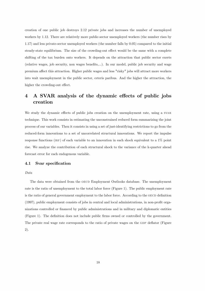
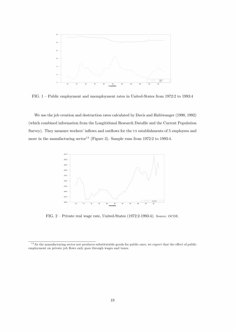
The data were obtained from the oecd Employment Outlooks database. The unemployment

rate is the ratio of unemployment to the total labor force (Figure 1). The public employment rate

is the ratio of general government employment to the labor force. According to the oecd definition

(1997), public employment consists of jobs in central and local administrations, in non-profit orga-

nizations controlled or financed by public administrations and in military and diplomatic entities

(Figure 1). The definition does not include public firms owned or controlled by the government.

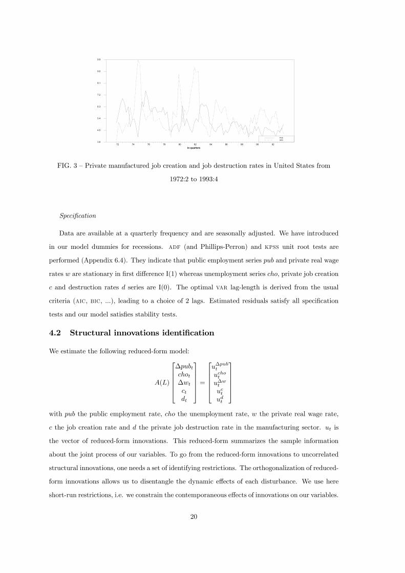
The private real wage rate corresponds to the ratio of private wages on the gdp deflator (Figure

2).

18

in quarters72 74 76 78 80 82 84 86 88 90 92

4

6

8

10

12

14

16

PUBLICUNR

FIG. 1 — Public employment and unemployment rates in United-States from 1972:2 to 1993:4

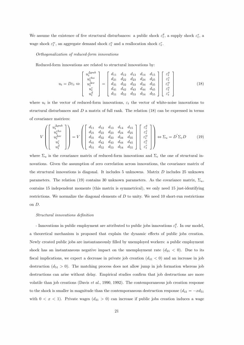
We use the job creation and destruction rates calculated by Davis and Haltiwanger (1990, 1992)

(which combined information from the Longitidunal Research Datafile and the Current Population

Survey). They measure workers’ inflows and outflows for the us establishments of 5 employees and

more in the manufacturing sector14 (Figure 3). Sample runs from 1972:2 to 1993:4.

trimestres72 74 76 78 80 82 84 86 88 90 92

235.0

237.5

240.0

242.5

245.0

247.5

250.0

252.5

255.0

257.5

SALAIRES

FIG. 2 — Private real wage rate, United-States (1972:2-1993:4). Source: OCDE.

14As the manufacturing sector not produces substitutable goods for public ones, we expect that the effect of publicemployment on private job flows only goes through wages and taxes.

19

in quarters72 74 76 78 80 82 84 86 88 90 92

3.6

4.5

5.4

6.3

7.2

8.1

9.0

9.9

POSNEG

FIG. 3 — Private manufactured job creation and job destruction rates in United States from

1972:2 to 1993:4

Specification

Data are available at a quarterly frequency and are seasonally adjusted. We have introduced

in our model dummies for recessions. adf (and Phillips-Perron) and kpss unit root tests are

performed (Appendix 6.4). They indicate that public employment series pub and private real wage

rates w are stationary in first difference I(1) whereas unemployment series cho, private job creation

c and destruction rates d series are I(0). The optimal var lag-length is derived from the usual

criteria (aic, bic, ...), leading to a choice of 2 lags. Estimated residuals satisfy all specification

tests and our model satisfies stability tests.

4.2 Structural innovations identification

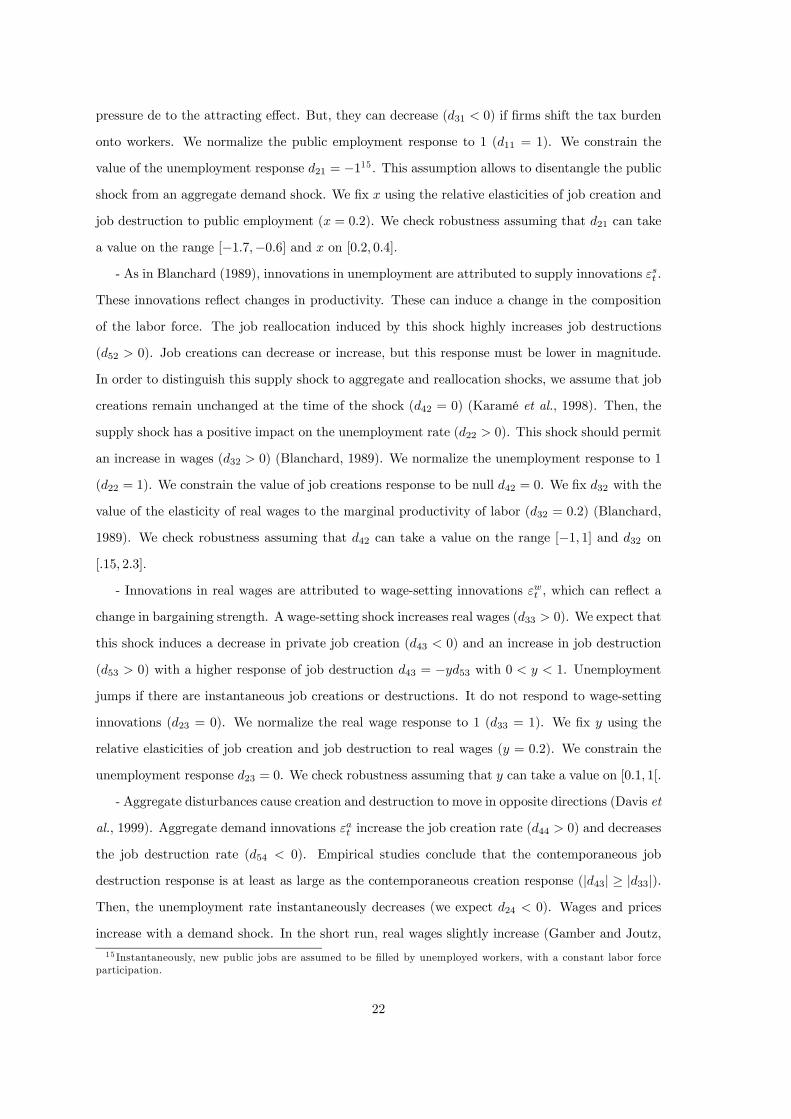
We estimate the following reduced-form model:

A(L)

∆pubtchot∆wt

ctdt

=u∆pubt

uchot

u∆wtuctudt

with pub the public employment rate, cho the unemployment rate, w the private real wage rate,

c the job creation rate and d the private job destruction rate in the manufacturing sector. ut is

the vector of reduced-form innovations. This reduced-form summarizes the sample information

about the joint process of our variables. To go from the reduced-form innovations to uncorrelated

structural innovations, one needs a set of identifying restrictions. The orthogonalization of reduced-

form innovations allows us to disentangle the dynamic effects of each disturbance. We use here

short-run restrictions, i.e. we constrain the contemporaneous effects of innovations on our variables.

20

We assume the existence of five structural disturbances: a public shock εgt , a supply shock εst , a

wage shock εwt , an aggregate demand shock εat and a reallocation shock ε

rt .

Orthogonalization of reduced-form innovations

Reduced-form innovations are related to structural innovations by:

ut = Dεt ⇔

u∆pubt

uchot

u∆wtuctudt

=

d11 d12 d13 d14 d15d21 d22 d23 d24 d25d31 d32 d33 d34 d35d41 d42 d43 d44 d45d51 d52 d53 d54 d55

εgtεstεwtεatεrt

(18)

where ut is the vector of reduced-form innovations, εt the vector of white-noise innovations to

structural disturbances and D a matrix of full rank. The relation (18) can be expressed in terms

of covariance matrices:

V

u∆pubt

uchot

u∆wtuctudt

= V

d11 d12 d13 d14 d15d21 d22 d23 d24 d25d31 d32 d33 d34 d35d41 d42 d43 d44 d45d51 d52 d53 d54 d55

εgtεstεwtεatεrt

⇔ Σu = D

0ΣεD (19)

where Σu is the covariance matrix of reduced-form innovations and Σε the one of structural in-

novations. Given the assumption of zero correlation across innovations, the covariance matrix of

the structural innovations is diagonal. It includes 5 unknowns. Matrix D includes 25 unknown

parameters. The relation (19) contains 30 unknown parameters. As the covariance matrix, Σu,

contains 15 independent moments (this matrix is symmetrical), we only need 15 just-identifying

restrictions. We normalize the diagonal elements of D to unity. We need 10 short-run restrictions

on D.

Structural innovations definition

- Innovations in public employment are attributed to public jobs innovations εgt . In our model,

a theoretical mechanism is proposed that explain the dynamic effects of public jobs creation.

Newly created public jobs are instantaneously filled by unemployed workers: a public employment

shock has an instantaneous negative impact on the unemployment rate (d21 < 0). Due to its

fiscal implications, we expect a decrease in private job creation (d41 < 0) and an increase in job

destruction (d51 > 0). The matching process does not allow jump in job formation whereas job

destructions can arise without delay. Empirical studies confirm that job destructions are more

volatile than job creations (Davis et al., 1990, 1992). The contemporaneous job creation response

to the shock is smaller in magnitude than the contemporaneous destruction response (d41 = −xd51with 0 < x < 1). Private wages (d31 > 0) can increase if public jobs creation induces a wage

21

pressure de to the attracting effect. But, they can decrease (d31 < 0) if firms shift the tax burden

onto workers. We normalize the public employment response to 1 (d11 = 1). We constrain the

value of the unemployment response d21 = −115. This assumption allows to disentangle the publicshock from an aggregate demand shock. We fix x using the relative elasticities of job creation and

job destruction to public employment (x = 0.2). We check robustness assuming that d21 can take

a value on the range [−1.7,−0.6] and x on [0.2, 0.4].

- As in Blanchard (1989), innovations in unemployment are attributed to supply innovations εst .

These innovations reflect changes in productivity. These can induce a change in the composition

of the labor force. The job reallocation induced by this shock highly increases job destructions

(d52 > 0). Job creations can decrease or increase, but this response must be lower in magnitude.

In order to distinguish this supply shock to aggregate and reallocation shocks, we assume that job

creations remain unchanged at the time of the shock (d42 = 0) (Karamé et al., 1998). Then, the

supply shock has a positive impact on the unemployment rate (d22 > 0). This shock should permit

an increase in wages (d32 > 0) (Blanchard, 1989). We normalize the unemployment response to 1

(d22 = 1). We constrain the value of job creations response to be null d42 = 0. We fix d32 with the

value of the elasticity of real wages to the marginal productivity of labor (d32 = 0.2) (Blanchard,

1989). We check robustness assuming that d42 can take a value on the range [−1, 1] and d32 on

[.15, 2.3].

- Innovations in real wages are attributed to wage-setting innovations εwt , which can reflect a

change in bargaining strength. A wage-setting shock increases real wages (d33 > 0). We expect that

this shock induces a decrease in private job creation (d43 < 0) and an increase in job destruction

(d53 > 0) with a higher response of job destruction d43 = −yd53 with 0 < y < 1. Unemployment

jumps if there are instantaneous job creations or destructions. It do not respond to wage-setting

innovations (d23 = 0). We normalize the real wage response to 1 (d33 = 1). We fix y using the

relative elasticities of job creation and job destruction to real wages (y = 0.2). We constrain the

unemployment response d23 = 0. We check robustness assuming that y can take a value on [0.1, 1[.

- Aggregate disturbances cause creation and destruction to move in opposite directions (Davis et

al., 1999). Aggregate demand innovations εat increase the job creation rate (d44 > 0) and decreases

the job destruction rate (d54 < 0). Empirical studies conclude that the contemporaneous job

destruction response is at least as large as the contemporaneous creation response (|d43| ≥ |d33|).Then, the unemployment rate instantaneously decreases (we expect d24 < 0). Wages and prices

increase with a demand shock. In the short run, real wages slightly increase (Gamber and Joutz,

15 Instantaneously, new public jobs are assumed to be filled by unemployed workers, with a constant labor forceparticipation.

22

1993) or decrease (Blanchard, 1989). As we normalize the job creation response to 1 (d44 = 1), the

job destruction response must be higher than 1 in absolute value. We constrain its value at the

opposite of the value of the ratio between the standard errors of destruction and creation series

(d54 = −1.55) (Karamé et al., 1998). We fix d34 using the elasticity of real wages to job creations(d34 = 0.07). Note that using a negative value would have minor effects. We check robustness

assuming that d54 can take a value on the range [−4,−1].- Reallocation disturbances cause creation and destruction to move in the same direction (Davis

et al., 1999). Reallocation innovations εrt increase job destruction (d55 > 0) and job creation

(d45 ≥ 0). The contemporaneous job creation response to a reallocation innovation is smaller inmagnitude than the contemporaneous destruction response (|d55| ≥ |d45|). As we normalize the jobdestruction response to 1 (d55 = 1), the job creation response must be lower or equal to 1 (Karamé

et al., 1998). We assume that the contemporaneous response of job creation is the same as the job

destruction response (d45 = 1). Then, a reallocation shock has no impact on the unemployment

rate (d25 = 0). We check robustness assuming that d45 can take a value on the range [0, 1].

Matrix D reads:

D =

1 d12 d13 d14 d15−1.7 1 0 d24 0d31 0.2 1 0.07 d35

−0.2d51 0 −0.2d53 1 1d51 d52 d53 −1.55 1

4.3 Results

We report in Appendix 6.5 the impulse response functions of public employment, unemployment,

private job creations and destructions rates, i.e. the dynamic response of the level16 of each of the

endogenous variables to innovations in each of the four structural disturbances. Each figure gives

both point estimates and one-standard deviation bands obtained by bootstrap simulations.

Impulse Response Functions

- The dynamic effects of a public shock are characterized on the first graph (Graph 8). A

one-standard deviation shock leads to a decrease in job creations of 0.05 percent and to an in-

crease in job destructions of 0.254 percent. As new public jobs are created, the shock induces a

significative decrease in unemployment of 0.06 percent. Due to instantaneous destructions and to

the disincentives to create private jobs, private employment is reduced. This makes the private

job creation rate increase of 0.135 percent in the third quarter. Then job creations return to their

equilibrium value and the effects are not significantly different from zero after the fourth quarter.16As public employment rate is I(1), we report the accumulated impulse response function of public employment

to innovations in each structural disturbance.

23

Due to these private job creations, unemployment decreases of 0.151 percent in the sixth quarter.

Then it reaches its steady state value and there are no significant effect after 2 years. This shock

significantly increases public employment growth. So a public shock has a significative negative

impact on unemployment in the short run. The mean adjustment time of unemployment to a

public shock is 14 quarters (3.5 years). As in our model, firms shift the tax burden onto workers:

private real wages decline of 0.626 percent, but not significantly.

- The dynamic effects of a supply shock are characterized on the second graph (Graph 9). A one-

standard deviation shock leads to an increase in job destructions 0.290 percent and a constrained

null impact on job creations. This makes unemployment increase of 0.135 percent (Blanchard,

1989, Blanchard and Quah, 1989, Gamber et al., 1993). Then job creations increase of 0.183 in the

third quarter (this supply impulse can be interpreted as a labor recomposing effect). Job creations

return to their equilibrium value and the effects are no more significant after 6 quarters. Public

employment growth increases of 0.04, but its response is not significantly different from zero after

2 quarters. Although public employment is in first difference, supply shock makes it return to its

steady-state value in the long run. Supply innovations decrease more nominal prices than nominal

wages. So, real wages increase but this effect is not significant (Blanchard, 1989).

- The dynamic effects of a wage-setting shock are characterized on the third graph (Graph

10). A one-standard deviation shock leads to a decrease in job creations of 0.041 percent and

an increase of job destructions of 0.206 percent in the first quarter. Then, private job creations

increase of 0.089 percent in the second quarter, but these responses are not statistically significant.

By assumption, unemployment instantaneously do not respond to the wage-setting shock, then

it decreases, although not significantly so (Blanchard, 1989). This shock significantly increases

real wages of 1.008 percent in the first quarter. A wage-setting makes public employment growth

increase, but this effect is not statistically different from zero.

- The dynamic effects of a positive aggregate demand shock are characterized on the fourth

graph (Graph 11). A one-standard deviation shock leads to an increase in job creations of 0.264

percent and an higher decrease in job destructions of 0.423 percent. So, it induces a decrease in

unemployment of 0.129 percent in the first quarter. Its effects on job flows are not significantly

different from zero after the shock (Karamé et al., 1998). In the first year, the aggregate shock leads

to a significant fall in unemployment of 0.215 percent. Then unemployment returns to its steady-

state value (this increase is not significantly different from zero after 2 years) (Blanchard, 1989,

Blanchard et al., 1989, Gamber et al., 1993). Aggregate disturbances make the public employment

growth increase of 0.032 percent (this rise is not significant after the first quarter). Aggregate

24

disturbances make real wages increase of 0.018 percent in the first quarter and then decrease,

though these effects are statistically insignificant (Blanchard, 1989).

- The dynamic effects of a reallocation shock are characterized on the fifth graph (Graph

12). A one-standard deviation shock leads to an increase in job creations and destructions of

0.284 percent. This shock has no instantaneous effect on unemployment as we’ve constrained it.

The impact on job creations are more persistent: job destructions quickly fall after the shock

whereas job creations slightly decrease (Karamé et al., 1998) (the effects on job creations are not

significantly different from zero after 6 quarters). This makes unemployment decrease, but without

any significant effect. Reallocation disturbances decrease the public employment growth but this

effect is not significantly different from zero. Reallocation disturbances tend to decrease real wages

but the response is statistically insignificant at all horizons.

Forecast Error Variance Decomposition

We report in Appendix 6.6 the contribution of each source of innovations to the variance of the n-

quarter ahead forecast error for each endogenous variable. Table 5 reports variance decompositions

for the first difference of public employment rate and for the levels of unemployment, job creation

and destruction rates.

- Innovations to aggregate demand, εat , and innovations to either labor supply or productivity,

εst , account for the most of the variance of unemployment in the short run: one quarter ahead,

they account for 43.16 percent and 47.3 percent of the variance of cho, respectively (Blanchard,

1989, Blanchard et al., 1989, Gamber et al., 1993, Dolado and Lopez-Salido, 1996). Eight quarters

ahead, εat still accounts for 53.73 percent of the variance of cho, whereas this proportion has

decreased for εst (16.14 percent). Innovations to public employment, εgt , account for a growing part

of the variance of cho (31.19 percent in the long run). In the long run, εat and εgt jointly explain

83.83 percent of the variance of cho. Reallocation innovations εrt not explain the variance of cho.

This is true by assumption for the one-quarter ahead variance: identification restriction imposes

that unemployment doesn’t respond to εrt . It is however true at longer horizons: in the long run,

they account for 3.33 percent of the variance of cho. Wage-setting innovations εwt not explain

the variance of cho. This is true by assumption for the one-quarter ahead variance: identification

restriction imposes that unemployment doesn’t respond to εwt . It is however true at longer horizons:

in the long run, they account for 1.8 percent of the variance of cho (Blanchard, 1989).

- Innovations to aggregate demand, εat , and reallocation innovations, εrt , account for the most

of the variance of private job creations in the short run: one quarter ahead, they account for 45.08

25

percent and 52.16 percent of the variance of c, respectively (Karamé et al., 1998). By assumption,

for the one-quarter ahead variance, supply innovations, εst , do not explain the variance of c. Eight

quarters ahead, εst accounts for 17.33 percent of the variance of the forecast error. In the long run,

εrt account for the most part of the variance: they explain 50 percent (Karamé et al., 1998). Eight

quarters ahead, public innovations, εgt , accounts for 9.1 percent of the variance of c. Wage-setting

innovations, εwt , explain 5 percent of the variance of c.

- Innovations to aggregate demand, εat , dominate all other innovations at all horizons: one

quarter ahead, they account for 39.69 percent of the variance of private job destructions and

ten years ahead, this proportion is 43.39 percent (Karamé et al., 1998). Innovations to public

employment, εgt , account for 14 percent of the variance of d at all horizons. So, a change in public

job creations changes incentives for private job destructions. Supply innovations, εst , contribute to

18 percent of the variance of d at all horizons.

- Wage-setting innovations, εwt , account for the most part of the variance of private real wage

rate in the short run: one quarter ahead, they account for 70 percent of the variance of w. Eight

quarters ahead, public innovations, εgt , account for 30 percent of the variance of the forecast error of

w. In the long run, εwt and εgt jointly explain 91 percent of the variance of w. This high contribution

of the public shock is convenient with our intuition: public jobs creation affects real wages but the

net effect is ambiguous.

- Public innovations, εgt , innovations to aggregate demand, εat , and reallocation innovations,

εrt , jointly account for 93.23 percent of the variance of public employment ten years ahead. One

quarter ahead, innovations to either labor supply or productivity, εst , account for 37.5 percent of

the variance of pub. This result reinforces our intuition: public job creations decisions partly are

due to innovations in labor supply, that make unemployment higher, in the very short term. In

long term, these are due to innovations in aggregate demand.

5 Conclusion

We use a dynamic matching model and study how public jobs creation affects workers’ decisions

to move on the labor market and private-sector firms’ job creation and destruction decisions.

Instantaneously, newly created public jobs are filled by the unemployed workers searching for a

public job. Thus, in the short run, the unemployment rate decreases and the public sector exerts an

attracting effect on private workers. Due to its fiscal implications, public jobs creation affects the

private-sector job creation and destruction decisions. The disincentives for private jobs creation

that distortive labor taxes generate make the unemployment rate increase. In the long run, the net

26

impact depends on the size of the public wage premium. With our calibration, public jobs creation

increases unemployment. The mean lag of the unemployment rate is close to 7 quarters. True

dynamic firms ’responses take time. Here, we assume that there is no adjustment cost. However,

there might be some inertia in private job creation and destruction decisions. Then, the adjustment

time of the unemployment rate should be slower.

As an empirical illustration, we estimate a svar model that focuses on the consequences of

public jobs creation on unemployment dynamics. We use us data on public employment, unem-

ployment, private-sector job creation and destruction rates, obtained from the oecd Employment

Outlooks, lrd and cps database. Sample runs from 1972:2 to 1993:4. We assume the existence

of four structural disturbances: a public shock, a supply shock, an aggregate shock and a real-

location shock. We use short-run restrictions in the spirit of Blanchard (1989), Karamé et al.

(1998) and Davis el al. (1999). Our results are consistent with the svar literature. We obtain

that the unemployment rate significantly decreases in the short-run with a public shock. It is true

by assumption for the one-quarter ahead: identification restriction imposes that unemployment

negatively responds to the public shock. But it also is true for six quarters-ahead17. Then the

unemployment rate reaches its steady-state value and there are no significant effect after 2 years.

The mean adjustment time of unemployment to a public shock is 3.5 years. This motivates a gov-

ernment response to a change in unemployment. Innovations in public employment account for a

significant part of the variance of private job destructions. Job creation dynamics are consistent to

those obtained in our theoretical model. Job destructions are more volatile than job creations and

they faster reach their steady-state value. In the same way, this is consistent with our matching

model. As we expected it, the response of private wages to a public shock is ambiguous. We ob-

tain a non statistically significant effect. This ambiguity comes from conflicting externalities that

public jobs creation generates: the attraction effect increases workers’ wage demands whereas tax

distortions reduce workers’ bargaining strength. The high contribution of the public shock to the

variance of private wages is consistent with our intuition: public employment affects private wages

but this effect is ambiguous. We can conclude that our svar model is a good empirical illustration

for our theoretical model. Note that the lack of data and the use of a bootstrap simulation of

one-standard deviation bands constrain the significativity of the impulse response functions. It

would be interesting to replicate this empirical exercise on other countries. However, we do not

have data on manufactured private-sector job creations and destructions (for France, we only have

17 In our model, the assumption of continuous wage renegociation not allows this result. The unemployment rateinstantaneously "jumps" with public jobs creation and private jobs destruction. Then it monotically reaches its newsteady-state value.

27

47 observations).

References

Algan, Y., Cahuc, P. and A. Zylberberg, 2002, Public Employment and Labor Market Perfor-

mances, Economic Policy 17, 8-65.

Blanchard, O.J., 1989, A traditional interpretation of macroeconomic fluctuations, American

Economic Review 79 (5),1146-1164.

Blanchard, O.J. and D. Quah, 1989, The dynamic effects of aggregate demand and supply

disturbances, American Economic Review 79 (4), 655-673.

Borjas, G.J., 2002, The wage structure and the sorting of workers into the public sector, NBER

Working papers 9313.

Davis, S.J., and Haltiwanger, J., 1990, Gross job creation and destruction: Microeconomic

evidence and macroeconomic implications, dans O. Blanchard and S. Fischer (eds.), NBER macro-

economics annual 1990, MIT Press, Cambridge, 123-168.

Davis, S.J., and J. Haltiwanger, 1992, Gross Job Creation, Gross Job Destruction, and Em-

ployment Reallocation, Quaterly Journal of Economics 107, 819-863.

Davis, S.J., and J. Haltiwanger, 1999, On the driving forces behind cyclical movements in

employment and job reallocation, American Economic Review 89 (5), 1234-1258.

Demekas, D.G. and Z.G. Kontolemis, 2000, Government Employment and Wages and Labour

Market Performance, Oxford Bulletin of Economics and Statistics 62, 391-415.

Dolado, J.J. and J.D. Lopez-Salido, 1996, Hysteresis and Economic Fluctuations, CEPR Dis-

cussion Paper n◦1334.

Edin, P.A. and B. Holmlund, 1997, Sectoral structural change and the state of the labour

market in Sweden, in: H. Siebert (ed.) Structural Change and Labour Market Flexibility, Mohr

Siedbeck, 89-121.

Elliot, B., Lucifora, C. and Meurs, D. (1998), Public sector pay in Europe, Macmillian, London.

Gamber, E.N. and F.L. Joutz, 1993, The dynamic effects of aggregate demand and supply

disturbances: Comment, American Economic Review 83 (5), 1387-1393.

Hamermesh, D., 1993, Labor Demand, Princeton University Press.

Holmlund, B., 1997, Macroeconomic Implications of Cash Limits in the Public Sector, Eco-

nomica 64, 49-62.

Johansen, 1988, Statistical Analysis of Cointegration Vectors, Journal of Economic Dynamics

and Control 12, 231-254.

28

Karamé F. and F. Mihoubi, 1998, Analyse structurelle des processus de création et de suppres-

sion d’emplois, Document d’Etudes de la DARES, n◦21.

Malley, J. and T. Moutos, 2001, Government employment and unemployment: With one hand

giveth the other taketh, Working Paper, University of Glasgow.

Mortensen, D.T. and C.A. Pissarides, 1994, Job creation and job destruction in the theory of

unemployment, Review of Economic Studies 61, 397-415.

Mortensen, D.T. and C.A. Pissarides, 1999, New developments in Models of Search in the Labor

Market, in: Ashenfelter, O. and Card, D. (eds.), Handbook of Labor Economics 3B, Elsevier Science

Publisher, Chap 39.

OCDE (1997), La mesure de l’emploi public dans les pays de l’OCDE. Sources, méthodes et

résultats, OCDE Document de Travail, GD(97)932.

Pissarides, C.A., 1996, Are employment tax cuts the answer to Europe’s unemployment prob-

lem, Working Paper, London School of Economics.

Pissarides, C.A., 2000, Equilibrium Unemployment Theory, second edition, Cambridge, MA:

MIT Press.

29

6 Appendix

6.1 Phase diagram

In Section 2.5, we present the out-of steady-state dynamics of the unemployment rate u(t). We

propose here to use a graphical method in order to illustrate the stability of our solution. With

jump variables, the two differential equations (3) and (2) of our model read:½u(t) = qpF (R)(1− lg − ug(t)) + qglg − θm(θ) (u(t)− ug(t))− gug(t)ug(t) = qglg − gug(t)

And can be rewritten:·u(t)ug(t)

¸=

·−θm(θ) θm(θ)− qpF (R)− g0 −g

¸ ·u(t)ug(t)

¸+

·qpF (R)(1− lg) + qglg

qglg

¸The diagonal matrix of eigenvalues D is given by

D =

−2(θm(θ) + g) +p2θm(θ)g

20

0−p2θm(θ)g

2

The negative sign of both eigenvalues confirm that the system is stable (Graph 5).

First case

The locus of points for which u equals 0 is the upward-sloping line ug =θm(θ)u− qpF (R)(1− lg)− qglg

θm(θ)− qpF (R)− g,

under the constraint θm(θ) − qpF (R) − g > 018 . The u = 0 crosses the horizontal axis at point

u =qpF (R)(1− lg) + qglg

θm(θ). If we start at a point on the u = 0 schedule and increase u a bit,

then the right-hand side of the expression for u decreases. Hence, u becomes negative and u is

decreasing in that region. The arrows in this region point south. A symmetric argument implies

that the arrows point north for points to the right of the u = 0 schedule (Graph 5).

The ug(t) = 0 locus is given by u∗g =qglgg, a vertical line. The expression for ug implies that if

ug rises, then ug decreases. Hence, to the right of the ug = 0 locus, ug is negative, and the arrows

point west. The arrows point east for points to the left of the ug = 0 schedule (Graph 5).

The steady state is the point at which the two loci cross, a condition that corresponds in this

case to u∗ = u∗g +

qpF (R)(1− lg − u∗g)θm(θ)

u∗g =qglgg

18This is the case of our model.

30

0=gu&

gu

u

*u

0=u&

Stable arm

Stable arm

x0

u

*gu

GRAPH. 5 — The phase diagram in the first stable case

Second case

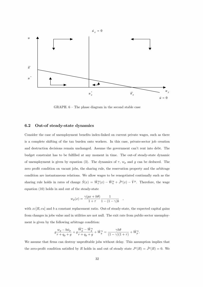
The locus of points for which u equals 0 is the downward-sloping line ug =θm(θ)u− qpF (R)(1− lg)− qglg

θm(θ)− qpF (R)− g,

under the constraint θm(θ) − qpF (R) − g < 0. The u = 0 schedule crosses the horizontal axis at

point u =qpF (R)(1− lg) + qglg

θm(θ)and the vertical axis at point ug = −qpF (R)(1− lg) + qglg

θm(θ)− qpF (R)− g. As

previously, the ug(t) = 0 locus is given by u∗g =qglgg, a vertical line. In the case u∗g < ug, the

system is stable as for any initial values of u and ug, the dynamics of the system takes it back to

the steady state (Graph 6). In the case u∗g > ug, the two loci do not cross. There is no steady

state.

31

gu

*u

u

*gu

0=u&gu

0=gu&

u

GRAPH. 6 — The phase diagram in the second stable case

6.2 Out-of steady-state dynamics

Consider the case of unemployment benefits index-linked on current private wages, such as there

is a complete shifting of the tax burden onto workers. In this case, private-sector job creation

and destruction decisions remain unchanged. Assume the government can’t rent into debt. The

budget constraint has to be fulfilled at any moment in time. The out-of steady-state dynamic

of unemployment is given by equation (3). The dynamics of τ , wp and g can be deduced. The

zero profit condition on vacant jobs, the sharing rule, the reservation property and the arbitrage

condition are instantaneous relations. We allow wages to be renegotiated continually such as the

sharing rule holds in rates of change S(x) = W pe (x) − W p

u + Jp(x) − V p. Therefore, the wage

equation (10) holds in and out of the steady-state

wp(x) =γ(px+ hθ)

1 + τ

1

1− (1− γ)b,

with xε]R, eu] and b a constant replacement ratio. Out-of steady-state, the expected capital gains

from changes in jobs value and in utilities are not null. The exit rate from public-sector unemploy-

ment is given by the following arbitrage condition:

gwg − bwp

r + qg + g+ g

W eg − Wu

g

r + qg + g+ Wu

g =γhθ

(1− γ)(1 + τ)+ Wu

p .

We assume that firms can destroy unprofitable jobs without delay. This assumption implies that

the zero-profit condition satisfied by R holds in and out of steady state Jp(R) = Jp(R) = 0. We

32

also assume that firms can open and close vacancies without delay. This assumption implies that

the zero-profit condition for new vacancies holds in and out of steady state V p = V p = 0. We

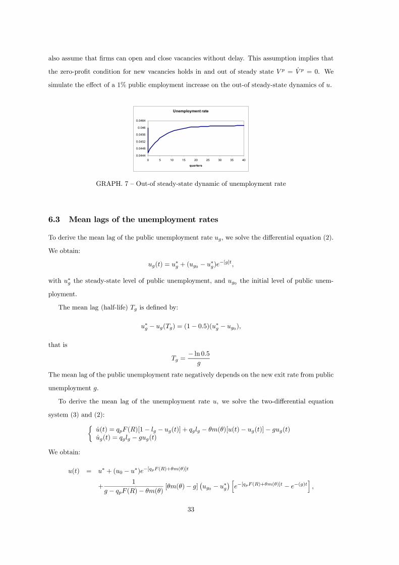
simulate the effect of a 1% public employment increase on the out-of steady-state dynamics of u.

Unemployment rate

0.0444

0.0448

0.0452

0.0456

0.046

0.0464

0 5 10 15 20 25 30 35 40

quarters

GRAPH. 7 — Out-of steady-state dynamic of unemployment rate

6.3 Mean lags of the unemployment rates

To derive the mean lag of the public unemployment rate ug, we solve the differential equation (2).

We obtain:

ug(t) = u∗g + (ug0 − u∗g)e−[g]t,

with u∗g the steady-state level of public unemployment, and ug0 the initial level of public unem-

ployment.

The mean lag (half-life) Tg is defined by:

u∗g − ug(Tg) = (1− 0.5)(u∗g − ug0),

that is

Tg =− ln 0.5

g

The mean lag of the public unemployment rate negatively depends on the new exit rate from public

unemployment g.

To derive the mean lag of the unemployment rate u, we solve the two-differential equation

system (3) and (2):½u(t) = qpF (R)[1− lg − ug(t)] + qglg − θm(θ)[u(t)− ug(t)]− gug(t)ug(t) = qglg − gug(t)

We obtain:

u(t) = u∗ + (u0 − u∗)e−[qpF (R)+θm(θ)]t

+1

g − qpF (R)− θm(θ)[θm(θ)− g]

¡ug0 − u∗g

¢ he−[qpF (R)+θm(θ)]t − e−(g)t

i,

33

with u∗ and u∗g the steady-state levels of total and public unemployment, and u0 and ug0 the initial

levels of total and public unemployment, respectively.

The mean lag T is given by:

u∗ − u(T ) = (1− 0.5)(u∗ − u0).

The properties of Tg and T are sum-up in Table 2.

TAB. 2 — Mean lagsr qg qp γ z

T(g) — — — 0 +

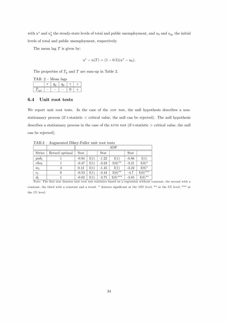
6.4 Unit root tests

We report unit root tests. In the case of the adf test, the null hypothesis describes a non-

stationnary process (if t-statistic < critical value, the null can be rejected). The null hypothesis

describes a stationnary process in the case of the kpss test (if t-statistic > critical value, the null

can be rejected).

TAB.3 — Augmented Dikey-Fuller unit root testsADF

Séries Retard optimal Stat Stat Stat

pubt 1 -0.94 I(1) -1.22 I(1) -0.86 I(1)chot 1 -0.47 I(1) -3.23 I(0)∗∗ -3.21 I(0)∗

wt 3 0.12 I(1) -1.45 I(1) -3.22 I(0)∗

ct 0 -0.53 I(1) -3.44 I(0)∗∗ -4.7 I(0)∗∗∗

dt 1 -0.82 I(1) -3.75 I(0)∗∗∗ -3.85 I(0)∗∗Note: The first stat denotes unit root test statistics based on a regression without constant, the second with a

constant, the third with a constant and a trend. * denotes significant at the 10% level, ** at the 5% level, *** at

the 1% level.

34

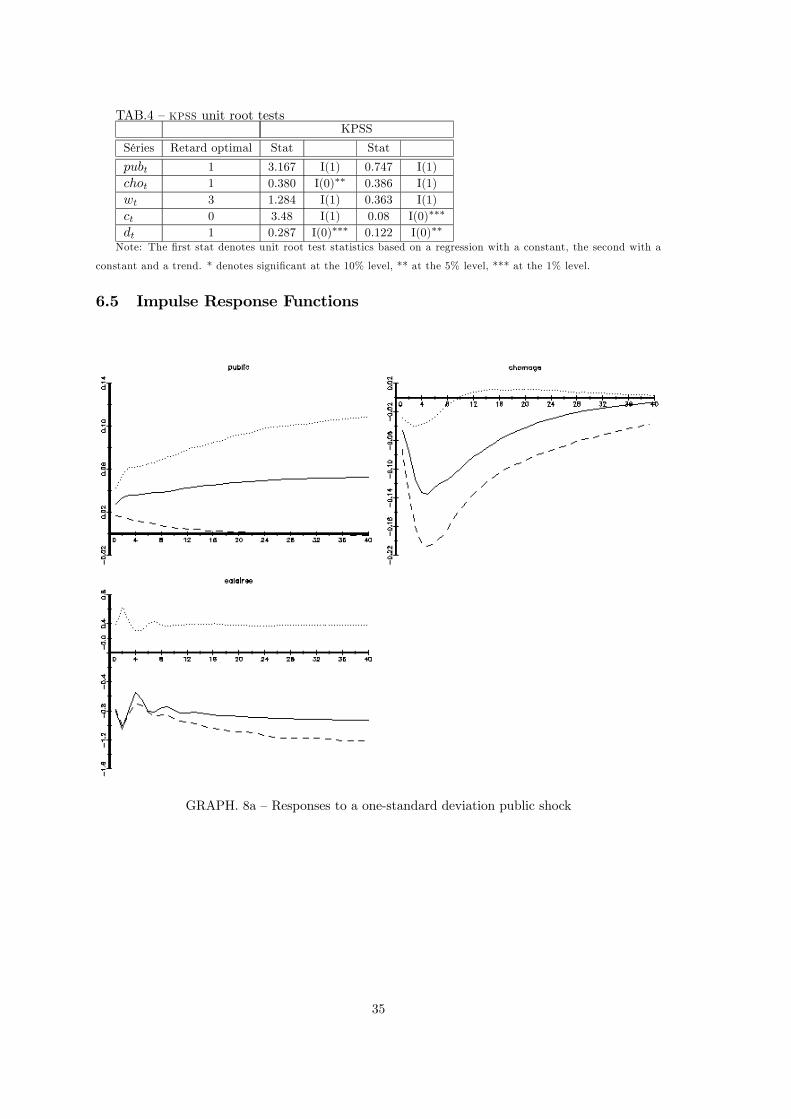
TAB.4 — kpss unit root testsKPSS

Séries Retard optimal Stat Stat

pubt 1 3.167 I(1) 0.747 I(1)chot 1 0.380 I(0)∗∗ 0.386 I(1)wt 3 1.284 I(1) 0.363 I(1)ct 0 3.48 I(1) 0.08 I(0)∗∗∗

dt 1 0.287 I(0)∗∗∗ 0.122 I(0)∗∗Note: The first stat denotes unit root test statistics based on a regression with a constant, the second with a

constant and a trend. * denotes significant at the 10% level, ** at the 5% level, *** at the 1% level.

6.5 Impulse Response Functions

GRAPH. 8a — Responses to a one-standard deviation public shock

35

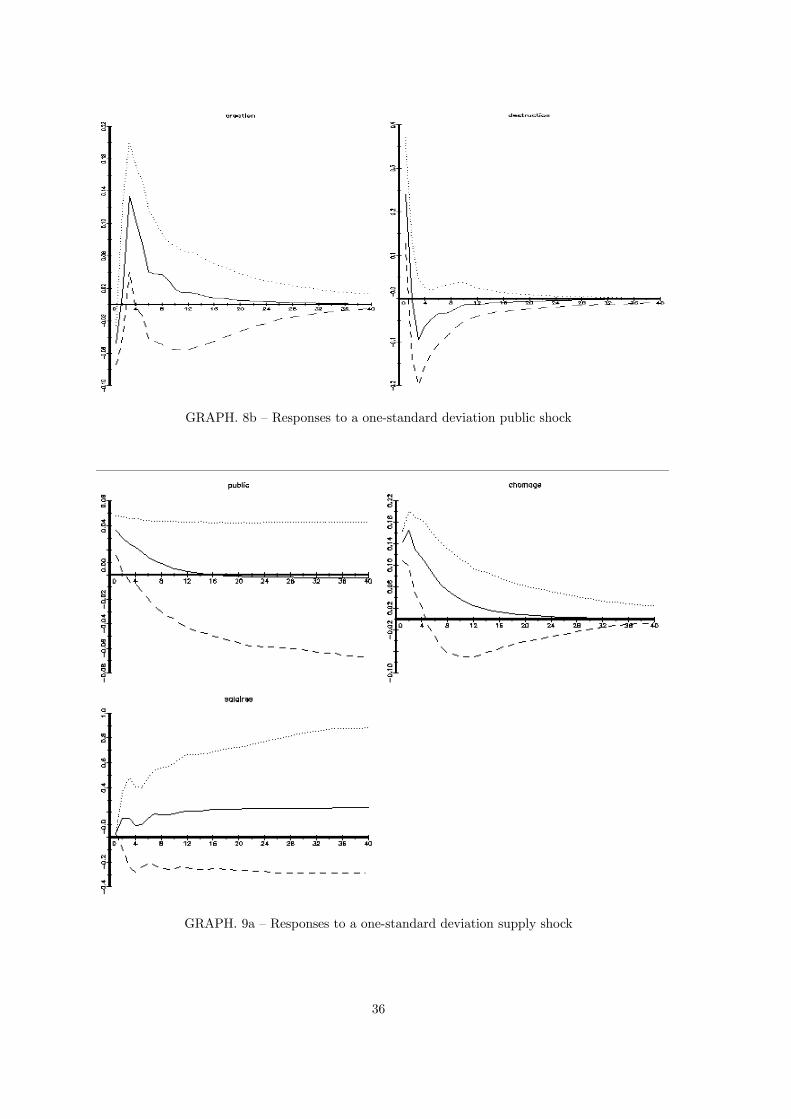
GRAPH. 8b — Responses to a one-standard deviation public shock

GRAPH. 9a — Responses to a one-standard deviation supply shock

36

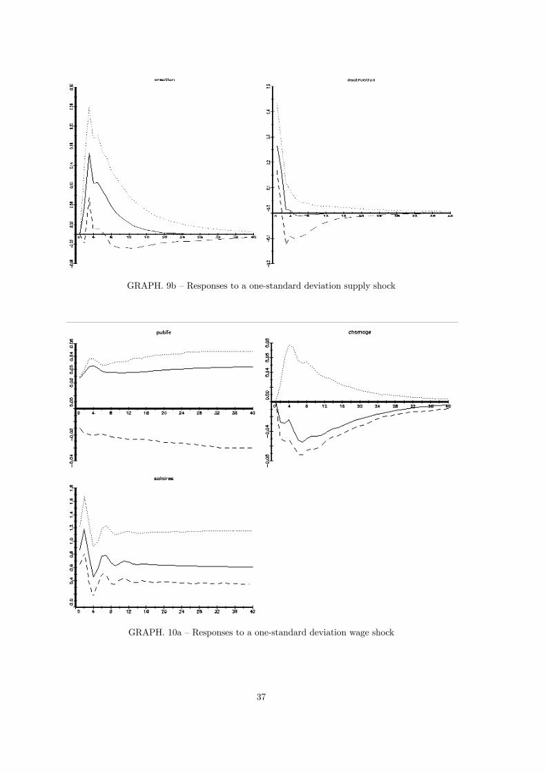
GRAPH. 9b — Responses to a one-standard deviation supply shock

GRAPH. 10a — Responses to a one-standard deviation wage shock

37

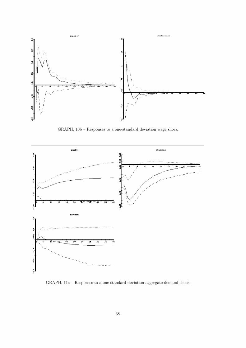
GRAPH. 10b — Responses to a one-standard deviation wage shock

GRAPH. 11a — Responses to a one-standard deviation aggregate demand shock

38

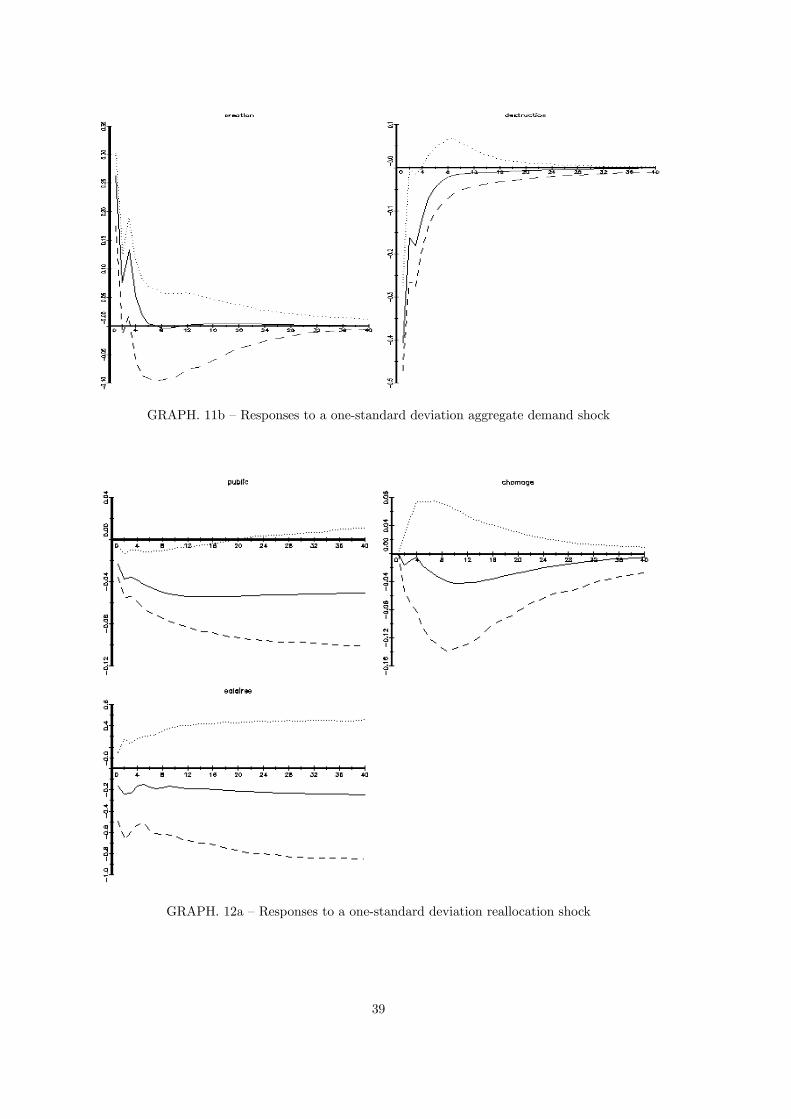
GRAPH. 11b — Responses to a one-standard deviation aggregate demand shock

GRAPH. 12a — Responses to a one-standard deviation reallocation shock

39

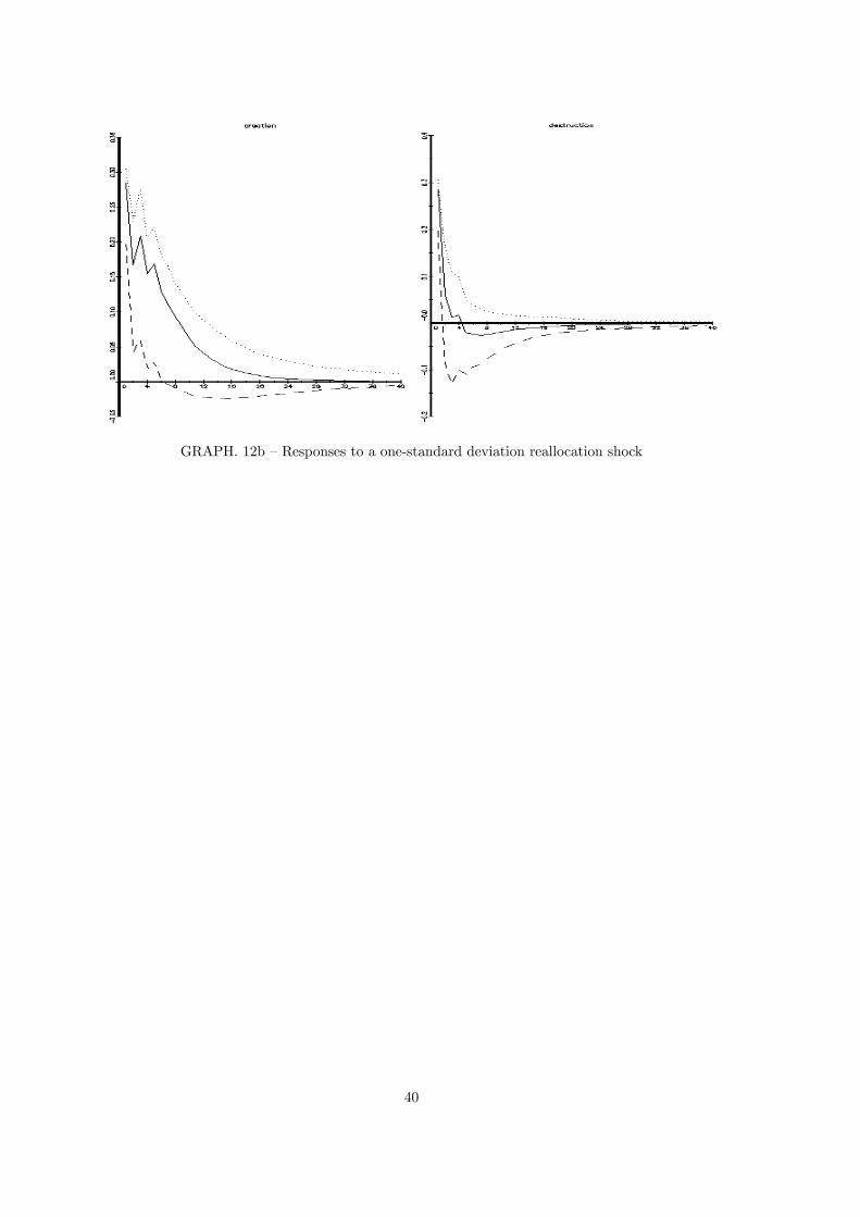
GRAPH. 12b — Responses to a one-standard deviation reallocation shock

40

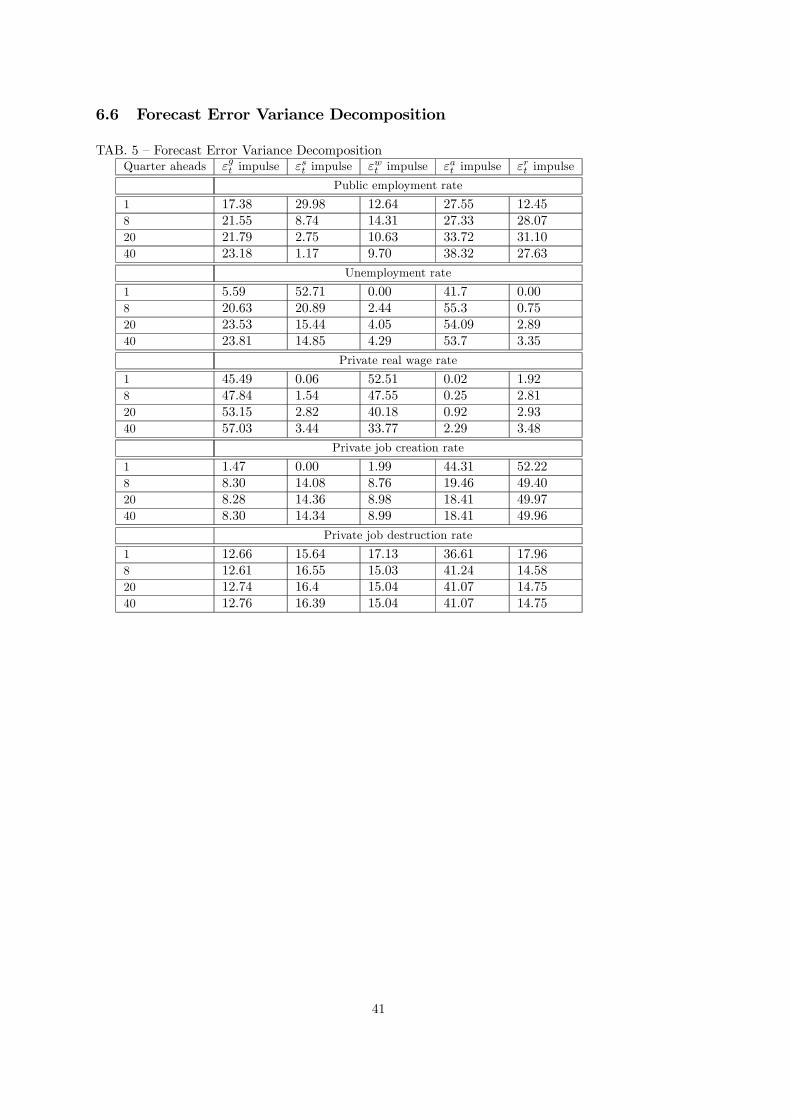
6.6 Forecast Error Variance Decomposition

TAB. 5 — Forecast Error Variance DecompositionQuarter aheads εgt impulse εst impulse εwt impulse εat impulse εrt impulse

Public employment rate

1 17.38 29.98 12.64 27.55 12.458 21.55 8.74 14.31 27.33 28.0720 21.79 2.75 10.63 33.72 31.1040 23.18 1.17 9.70 38.32 27.63

Unemployment rate

1 5.59 52.71 0.00 41.7 0.008 20.63 20.89 2.44 55.3 0.7520 23.53 15.44 4.05 54.09 2.8940 23.81 14.85 4.29 53.7 3.35

Private real wage rate

1 45.49 0.06 52.51 0.02 1.928 47.84 1.54 47.55 0.25 2.8120 53.15 2.82 40.18 0.92 2.9340 57.03 3.44 33.77 2.29 3.48

Private job creation rate

1 1.47 0.00 1.99 44.31 52.228 8.30 14.08 8.76 19.46 49.4020 8.28 14.36 8.98 18.41 49.9740 8.30 14.34 8.99 18.41 49.96

Private job destruction rate

1 12.66 15.64 17.13 36.61 17.968 12.61 16.55 15.03 41.24 14.5820 12.74 16.4 15.04 41.07 14.7540 12.76 16.39 15.04 41.07 14.75

41