Documents de Travail du Centre d’Economie de la … codes: O15,Q54. ... Documents de Travail du Centre d'Economie de la Sorbonne - 2013.45. monthswithﬂoodeventswereHimachalPradesh,Haryana,Meghalaya,Pun-

Documents de Travail du Centre d’Economie de la Sorbonne

Climate Variability and Internal Migration:

A Test on Indian Inter-State Migration

Ingrid DALLMANN, Katrin MILLOCK

2013.45

Maison des Sciences Économiques, 106-112 boulevard de L'Hôpital, 75647 Paris Cedex 13 http://centredeconomiesorbonne.univ-paris1.fr/bandeau-haut/documents-de-travail/

ISSN : 1955-611X

Climate Variability and Internal Migration:A Test on Indian Inter-State Migration ∗

Ingrid Dallmann†

Katrin Millock‡

May 15, 2013

Abstract

We match migration data from the Indian census with climate data totest the hypothesis of climate variability as a push factor for internalmigration. The main contribution of the analysis is to introduce rele-vant meteorological indicators of climate variability, based on the stan-dardized precipitation index. Gravity-type estimations derived from autility maximization approach cannot reject the null hypothesis thatthe frequency of drought acts as a push factor on inter-state migrationin India. The effect is significant for both male and female migrationrates. Drought duration and magnitude as well as flood events arenever statistically significant.

JEL codes: O15, Q54.

Keywords: climate change, India, internal migration, PPML, SPI.

∗We thank Eric Strobl for providing climate data, including the SPI. We thank alsoCatherine Bros, Sudeshna Chattopadhyay, Miren Lafourcade and Céline Nauges for theirhelp and advice, as well as participants in the 2nd International Conference on Envi-ronment and Natural Resources Management in Developing and Transition Economies(enrmdte), in particular Simone Bertoli. Any errors or omissions are only the authors’responsibility, naturally. Financial support from the French National Research Agencygrant ANR-JCJC-0127-01 is gratefully acknowledged.†University Paris-Sud 11 (ADIS); [email protected]‡Paris School of Economics, CNRS, Centre d’Economie de la Sorbonne; millock@univ-

paris1.fr

1

Documents de Travail du Centre d'Economie de la Sorbonne - 2013.45

1 IntroductionNegative effects linked to climate change are more and more apparent, notonly through the increase in natural disasters that cause huge economic andhuman losses but also through its long-term consequences. But, does climatechange affect migration? According to a report issued by the UK GovernmentOffice for Science (2011) [19], the response is affirmative: environmentalchange will affect migration in the present and in the future, but the influencewill be principally through economic, social and political drivers. Climatevariability may have direct effects, causing injury, death, crop damage anddisruption of socio-economic activities, but also have indirect effects on theenvironment and the economy, hence inducing migration either directly orindirectly.

The purpose of this paper is to test the hypothesis that long-term climatevariability acts as a push-factor on internal migration. Specifically, we inves-tigate if the frequency, duration and magnitude of drought and flood eventshave induced inter-state migration flows in India. Since the environmentalfactor is not the only driver of migration, we control also for the most impor-tant social and economic drivers. In order to do so, we match data from theIndian census of 1991 and 2001 with climate data of the IntergovernmentalPanel on Climate Change (IPCC). The econometric specification is based ona random utility model. The estimation results show that the frequency ofdrought events has a significant impact on inter-state migration flows. Eachadditional month of drought in the origin state during the five years preced-ing the year of migration increases the bilateral migration rate by 0.9%. Therelative effect is rather small compared to the economic drivers of migration.In addition, barriers to inter-state migration have a much more importanteffect, as reflected in the low Indian inter-state migration rates.

The analysis contributes to a small but growing literature that analyzesthe link between migration and climate change. Amongst these studies,the definition of migration (net migration, out-migration, immigration), thechoice of the zone of study (rural-urban, local, internal, international, devel-oping and developed countries), the aggregation level, the theoretical model,the indicators of climate change and the empirical methodology vary signifi-cantly and, as a result, they are inconclusive and hardly comparable. Macroe-conomic studies on international migration flows such as Reuveny and Moore(2009) [36] and Coniglio and Pesce (2011) [13] show that both weather-relatednatural disasters and climate anomalies may (directly) induce increased mi-gration into OECD countries, as suggested by the theoretical predictions ofMarchiori and Schumacher (2011) [26]. Naudé (2008) [34] finds that the num-ber of natural disasters during the 5 years preceding migration has an indirect

2


but significant positive effect on net international migration in sub-SaharanAfrica from 1965 to 2005. Beine and Parsons (2012) [6] who include bothweather variables such as rainfall and temperature and natural disasters intheir analysis find no evidence that climate change would induce an increasein international migration flows. This result is compatible with householdlevel analyses, such as Gray (2009) [20] on data from the Andean Zone ofSouthern Ecuador. Gray (2009) finds that environmental factors influencelocal and internal migration, and that negative environmental conditions donot increase international migration necessarily, as predicted in the “envi-ronmental refugees” literature (Myers, 1997) [33]. International migrationimplies high costs that may be prohibitive for the poorest households thatare the most vulnerable to environmental conditions.

Some recent studies on environmentally induced internal migration con-cern a well-known historical episode, the Dust Bowl1 in the U.S. Great Plainsin the 1930’s. During this episode, weather and environmental conditionsplayed a significant role in explaining internal migration (Gutmann et al.,2005) [?]. Hornbeck (2012) [23] concludes that the Dust Bowl had an im-mediate substantial and persistent negative impact on the value and incomefrom farmlands (through soil erosion). The economy adjusted mainly throughmigration rather than through capital inflows or industrialization. Anotherstudy of urbanization, Barrios et al. (2006) [4] finds that rainfall variabilityhad an important impact on urbanization in sub-Saharan Africa, but not inthe other developing countries included in their sample.

The only existing studies on India have either analyzed cross-section data(Bhattacharya and Innes, 2008 [10]), focused on the indirect impact of climateon migration through its effect on agricultural yields (Viswanathan and Ku-mar, 2012 [43]) or used village data representing only some districts or states(Badiani and Safir, 2008 [3]). Bhattacharya and Innes (2008) [10] studied therelationship between population growth and environment in India, but themeasures used to proxy environmental deterioration - net vegetation cover -are endogenous and dependent on agricultural production and behaviour ofthe households, contrary to exogenous measures such as the rainfall or tem-perature. We thus extend the existing literature on Indian internal migrationby introducing new standardized exogenous measures of climate variabilityinto a gravity-type model of internal migration. In doing so we also con-tribute to the migration literature using gravity-type models (Karemera etal., 2000 [24], Mayda, 2010 [28], Van Lottum and Marks, 2010 [42], and inparticular Özden and Sewadeh, 2010 [35] on India).

1Dust storm series, considered an ecological catastrophe, that affected the U.S. andCanada great plains region during almost a decade in the 1930’s.

3


The relationship between climate change and migration is complex andmany questions arise: who will be affected by climate change induced migra-tion? Where and in which geographic space is this migration likely to occur?Will the migration be permanent or temporal? Which climatic conditionsare the more influential? Through which channels will migration occur? Andwhat will be its political implications? More detailed empirical and theoret-ical studies may clarify some of these questions. In this paper, we focus oninternal (inter-state) migration in India, since climate change induced migra-tion is more likely to occur within the internal borders of a country, becauseof migration costs, including legal barriers (Marchiori et al., 2012 [27], Beineand Parsons, 2012 [6]). In addition, low-income and lower-middle-incomecountries are also more vulnerable to climate change than high-income coun-tries (Stern, 2007 [40]; Government Office for Science, 2011 [19]) due to theirlower climate change adaptation capacity and their geographical location.

2 Inter-state migration and climate variabilityin India

Analyzing inter-state migration in India is particularly appropriate for astudy of internal migration because of the size of the Indian states (the equiv-alent of European states), and the heterogeneity among them, especially asregards demography and climate. India has a large variety of climate regions,ranging from tropical in the South to temperate and alpine in the HimalayanNorth. This variation is maybe greater than any other area of similar sizein the world. Nearly 75% of the annual rainfall is received during the mon-soon season (June to September). The main natural disasters in India aredrought, flood and tropical cyclones (Attri and Tyagi, 2010) [2]. India isalso considered by the Environmental Vulnerability Index as extremely vul-nerable, not only because of its climate vulnerability, but also because of itspopulation density. In fact, India is after China the second most populatedcountry in the world (1,210 million inhabitants in 2011 that represents 17.5%of the world population with only 2.4% of the world surface area), with apopulation growth between 2001 and 2011 of 17.6%, which exceeds the worldpopulation growth (12.9%) [12]. Its population is mainly rural, of 72.2 % in2001 (this represents 742.5 million people).2 Even if its rural population hasdropped in percentage since 1901 and with an accelerating rate from the1970’s and onwards, India remains a country with a low urbanisation level(Datta, 2006) [14]. Besides, the population densities contrast very much be-

2Indian Census: www.censusindia.gov.in

4


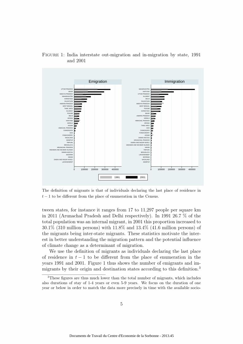
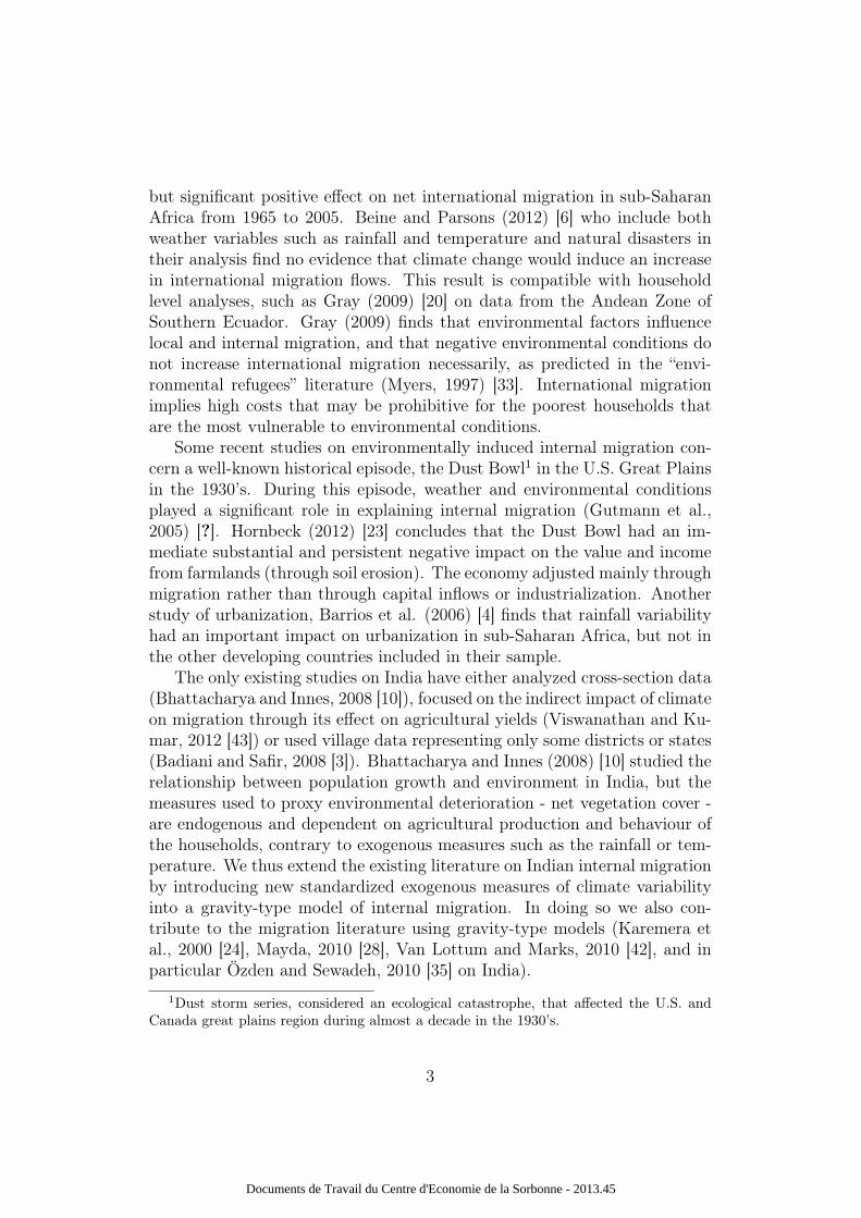
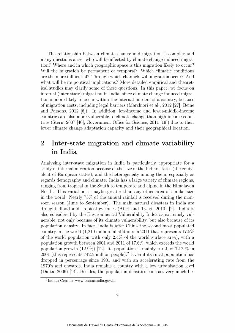
Figure 1: India interstate out-migration and in-migration by state, 1991and 2001

0 100000 200000 300000 400000 0 100000 200000 300000 400000

LAKSHADWEEP

DADRA AND NAGAR HAVELI

SIKKIM

MIZORAM

DAMAN AND DIU

ANDAMAN AND NICOBAR ISLANDS

ARUNACHAL PRADESH

MEGHALAYA

TRIPURA

MANIPUR

NAGALAND

PONDICHERRY

GOA

CHANDIGARH

HIMACHAL PRADESH

ASSAM

KERALA

HARYANA

ORISSA

DELHI

PUNJAB

GUJARAT

TAMIL NADU

WEST BENGAL

ANDHRA PRADESH

RAJASTHAN

KARNATAKA

MAHARASHTRA

MADHYA PRADESH

BIHAR

UTTAR PRADESH

MANIPUR

NAGALAND

MIZORAM

LAKSHADWEEP

MEGHALAYA

TRIPURA

SIKKIM



ARUNACHAL PRADESH

DAMAN AND DIU

ASSAM

PONDICHERRY

CHANDIGARH

GOA

TAMIL NADU

ORISSA

HIMACHAL PRADESH

KERALA

ANDHRA PRADESH

BIHAR

KARNATAKA

PUNJAB

WEST BENGAL

MADHYA PRADESH

RAJASTHAN

DELHI

GUJARAT

UTTAR PRADESH

HARYANA

MAHARASHTRA

Emigration Immigration

1991 2001

The definition of migrants is that of individuals declaring the last place of residence int− 1 to be different from the place of enumeration in the Census.

tween states, for instance it ranges from 17 to 11,297 people per square kmin 2011 (Arunachal Pradesh and Delhi respectively). In 1991 26.7 % of thetotal population was an internal migrant, in 2001 this proportion increased to30.1% (310 million persons) with 11.8% and 13.4% (41.6 million persons) ofthe migrants being inter-state migrants. These statistics motivate the inter-est in better understanding the migration pattern and the potential influenceof climate change as a determinant of migration.

We use the definition of migrants as individuals declaring the last placeof residence in t− 1 to be different from the place of enumeration in theyears 1991 and 2001. Figure 1 thus shows the number of emigrants and im-migrants by their origin and destination states according to this definition.3

3These figures are thus much lower than the total number of migrants, which includesalso durations of stay of 1-4 years or even 5-9 years. We focus on the duration of oneyear or below in order to match the data more precisely in time with the available socio-

5


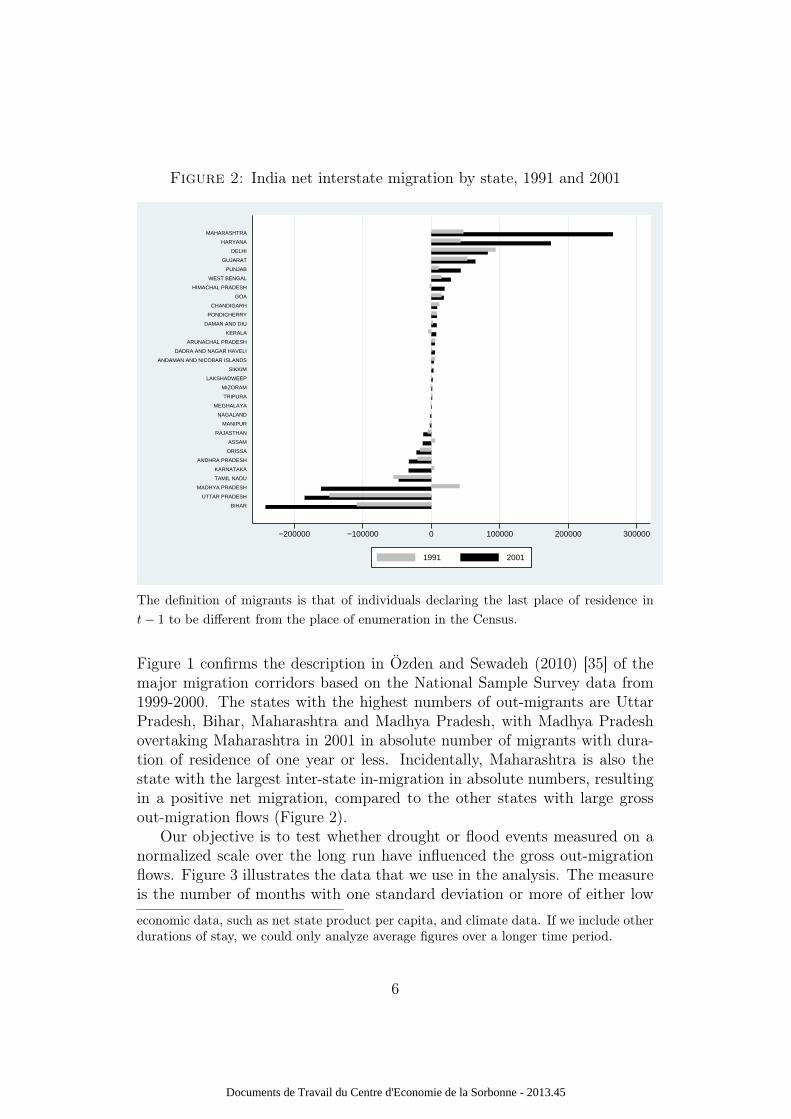
Figure 2: India net interstate migration by state, 1991 and 2001

−200000 −100000 0 100000 200000 300000

BIHAR

UTTAR PRADESH

MADHYA PRADESH

TAMIL NADU

KARNATAKA

ANDHRA PRADESH

ORISSA

ASSAM

RAJASTHAN

MANIPUR

NAGALAND

MEGHALAYA

TRIPURA

MIZORAM

LAKSHADWEEP

SIKKIM



ARUNACHAL PRADESH

KERALA

DAMAN AND DIU

PONDICHERRY

CHANDIGARH

GOA

HIMACHAL PRADESH

WEST BENGAL

PUNJAB

GUJARAT

DELHI

HARYANA

MAHARASHTRA

1991 2001

The definition of migrants is that of individuals declaring the last place of residence int− 1 to be different from the place of enumeration in the Census.

Figure 1 confirms the description in Özden and Sewadeh (2010) [35] of themajor migration corridors based on the National Sample Survey data from1999-2000. The states with the highest numbers of out-migrants are UttarPradesh, Bihar, Maharashtra and Madhya Pradesh, with Madhya Pradeshovertaking Maharashtra in 2001 in absolute number of migrants with dura-tion of residence of one year or less. Incidentally, Maharashtra is also thestate with the largest inter-state in-migration in absolute numbers, resultingin a positive net migration, compared to the other states with large grossout-migration flows (Figure 2).

Our objective is to test whether drought or flood events measured on anormalized scale over the long run have influenced the gross out-migrationflows. Figure 3 illustrates the data that we use in the analysis. The measureis the number of months with one standard deviation or more of either low

economic data, such as net state product per capita, and climate data. If we include otherdurations of stay, we could only analyze average figures over a longer time period.

6


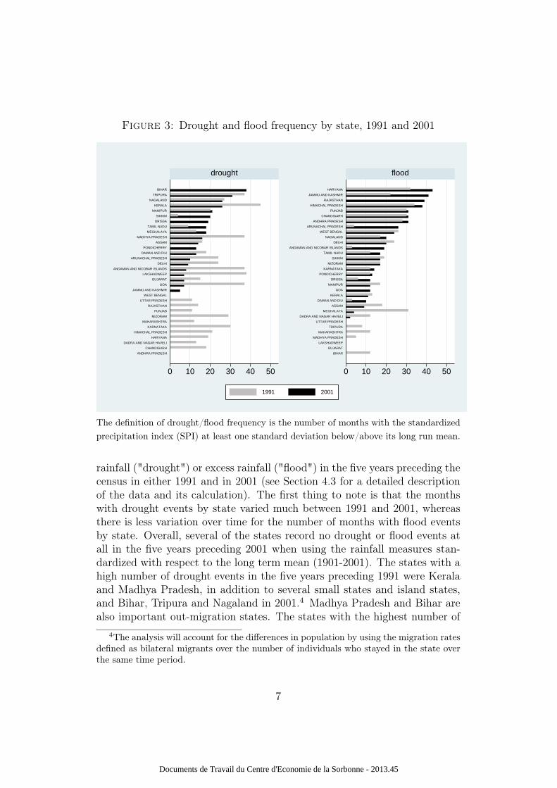
Figure 3: Drought and flood frequency by state, 1991 and 2001

0 10 20 30 40 50 0 10 20 30 40 50

ANDHRA PRADESH

CHANDIGARH


HARYANA

HIMACHAL PRADESH

KARNATAKA

MAHARASHTRA

MIZORAM

PUNJAB

RAJASTHAN

UTTAR PRADESH

WEST BENGAL

JAMMU AND KASHMIR

GOA

GUJARAT

LAKSHADWEEP


DELHI

ARUNACHAL PRADESH

DAMAN AND DIU

PONDICHERRY

ASSAM

MADHYA PRADESH

MEGHALAYA

TAMIL NADU

ORISSA

SIKKIM

MANIPUR

KERALA

NAGALAND

TRIPURA

BIHAR

BIHAR

GUJARAT

LAKSHADWEEP

MADHYA PRADESH

MAHARASHTRA

TRIPURA

UTTAR PRADESH


MEGHALAYA

ASSAM

DAMAN AND DIU

KERALA

GOA

MANIPUR

ORISSA

PONDICHERRY

KARNATAKA

MIZORAM

SIKKIM

TAMIL NADU


DELHI

NAGALAND

WEST BENGAL

ARUNACHAL PRADESH

ANDHRA PRADESH

CHANDIGARH

PUNJAB

HIMACHAL PRADESH

RAJASTHAN

JAMMU AND KASHMIR

HARYANA

drought flood

1991 2001

The definition of drought/flood frequency is the number of months with the standardizedprecipitation index (SPI) at least one standard deviation below/above its long run mean.

rainfall ("drought") or excess rainfall ("flood") in the five years preceding thecensus in either 1991 and in 2001 (see Section 4.3 for a detailed descriptionof the data and its calculation). The first thing to note is that the monthswith drought events by state varied much between 1991 and 2001, whereasthere is less variation over time for the number of months with flood eventsby state. Overall, several of the states record no drought or flood events atall in the five years preceding 2001 when using the rainfall measures stan-dardized with respect to the long term mean (1901-2001). The states with ahigh number of drought events in the five years preceding 1991 were Keralaand Madhya Pradesh, in addition to several small states and island states,and Bihar, Tripura and Nagaland in 2001.4 Madhya Pradesh and Bihar arealso important out-migration states. The states with the highest number of

4The analysis will account for the differences in population by using the migration ratesdefined as bilateral migrants over the number of individuals who stayed in the state overthe same time period.

7


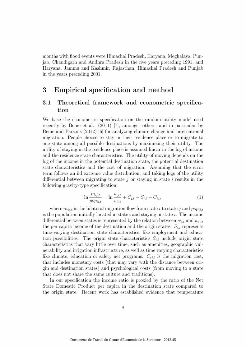
months with flood events were Himachal Pradesh, Haryana, Meghalaya, Pun-jab, Chandigarh and Andhra Pradesh in the five years preceding 1991, andHaryana, Jammu and Kashmir, Rajasthan, Himachal Pradesh and Punjabin the years preceding 2001.

3 Empirical specification and method

3.1 Theoretical framework and econometric specifica-tion

We base the econometric specification on the random utility model usedrecently by Beine et al. (2011) [7], amongst others, and in particular byBeine and Parsons (2012) [6] for analyzing climate change and internationalmigration. People choose to stay in their residence place or to migrate toone state among all possible destinations by maximizing their utility. Theutility of staying in the residence place is assumed linear in the log of incomeand the residence state characteristics. The utility of moving depends on thelog of the income in the potential destination state, the potential destinationstate characteristics and the cost of migration. Assuming that the errorterm follows an iid extreme value distribution, and taking logs of the utilitydifferential between migrating to state j or staying in state i results in thefollowing gravity-type specification:

lnmij,t

popii,t= ln

wj,t

wi,t

+ Sj,t − Si,t − Cij,t (1)

wheremij,t is the bilateral migration flow from state i to state j and popii,tis the population initially located in state i and staying in state i. The incomedifferential between states is represented by the relation between wj,t and wi,t,the per capita income of the destination and the origin states. Sj,t representstime-varying destination state characteristics, like employment and educa-tion possibilities. The origin state characteristics Si,t include origin statecharacteristics that vary little over time, such as amenities, geographic vul-nerability and irrigation infrastructure, as well as time varying characteristicslike climate, education or safety net programs. Cij,t is the migration cost,that includes monetary costs (that may vary with the distance between ori-gin and destination states) and psychological costs (from moving to a statethat does not share the same culture and traditions).

In our specification the income ratio is proxied by the ratio of the NetState Domestic Product per capita in the destination state compared tothe origin state. Recent work has established evidence that temperature

8


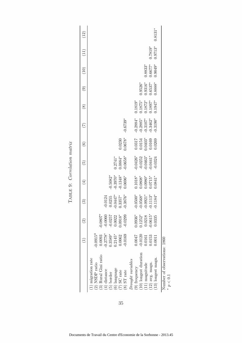
and rainfall affect income growth, although not always absolute levels ofincome (Dell et al., 2009 [16]; Barrios et al., 2010 [5]). Here we use theincome ratio, which is less correlated with climate variability in the originstate. Rather than studying the indirect effect of climate variability workingthrough income we aim at testing if there is a direct effect on migrationfrom the direct utility-decreasing effects of climate variability. As shown inthe correlation matrix (Table 9 in Appendix B) our main climate variable- frequency of droughts - has less than a 10 % correlation with the incomeratio. If there was concern that the correlation was larger, it would indeed bedifficult to identify a separate direct effect of climate variability on bilateralmigration flows.

The cost of migration is represented by distance, and a common borderor language between states. We also control for caste (or ethnic) similaritybetween states by controlling for the ratios of scheduled castes and scheduledtribes in the destination state compared to the origin state. The principalvariables of interest are the ones representing climate variability. Our hy-pothesis is that adverse weather events act as a push factor on migration. Inparticular, this is the case in developing countries where poor people do notmove by comparing origin and destination climate conditions but rather es-cape from adverse climate events that affect their well-being. Accordingly, allour variables representing climate variability act only in the origin state.5 Weinclude origin state fixed effects (Di) that are invariable in time to capturethe vulnerability of the geographic zone, especially mountains, low eleva-tion coasts and arid lands, but also to catch the effect of long-term climatechange adaptation strategies adopted by the state, such as irrigation infras-tructure. This dummy controls also for the states affected by the ArmedForces (Special Powers) Act of 1958. The Act gives special power to armedforces (military and air forces) in the so called “disturbed” areas. The statesand Union Territories affected are: Arunachal Pradesh, Assam, Manipur,Meghalaya, Mizoram, Nagaland and Tripura. These states have experiencedviolence that may have induced migration.

Destination state and time fixed effects (Djt) capture characteristics vary-ing in time like employment and education potentials in the destination state.

The resulting econometric specification is thus the following:5Lewer and Van den Berg (2008) [25] and Bodvarsson and Van den Berg (2009) [11]

discuss the potential sources of bias in the gravity model. One of them is that the presenceof unilateral variables, like the climate variables in this specification, can result in standarderror clustering. They cite Feenstra (2004) [18], who argues that adding fixed effectsdummies eliminates this bias.

9


lnmij,t

popii,t=a0 + a1 ln

wj,t−1

wi,t−1

+ a2 lnSCjt + 1

SCit + 1+ a3 ln

STjt + 1

STit + 1

+ a4 ln distij + a5borderij + a6languageij

+ a7

t∑t−5

climi,t +Di +Djt + uijt

(2)

whereState i: Origin state.State j: Destination state.mijt: Migration flow from state i to state j during

year t− 1 to t.popii,t Population of state i staying in the state during

year t− 1 to t.wj,t−1

wi,t−1: Ratio of the Net State Domestic Product per

capita in state j and in state i at time t− 1.SCit, SCjt: Scheduled caste rate in state i/j at time t.STit, STjt: Scheduled tribe rate in state i/j at time t.distij: Distance from state i to state j.borderij: Dummy variable for common border between

state i and j.languageij: Dummy variable for common language between

state i and j.climi,t: Frequency, duration or magnitude of

drought/flood in state i, during the fiveyears preceding t.

Di: Time-invariant fixed effect for state i.Djt: Destination-time fixed effect for state j.

The expected signs are: a1>0, a4<0, a5>0 and a6>0. All else equal, thelarger the differential of the per capita income between states, the larger theincentive to migrate.The relation of migration with distance is negative, sinceit proxies migration travel costs. Common border and language are viewedas facilitators for migration (or factors that reduce the cost of migrating).

We include an additional cost factor for migration in the form of differ-ences in scheduled caste and tribe ratios in the destination state compared

10


to the origin state, to account for similarity between states. Scheduled castesand tribes may be the most vulnerable parts of the population to climatevariability given that they often are day labourers and hence likely to be thefirst affected by climate events. These variables capture network effects inthe sense that, for an individual belonging to the scheduled castes (or tribes)population, moving to a state with a higher ratio of scheduled castes (ortribes) compared to the origin state would imply lower costs of migrationbecause of the network in the destination state, whereas moving to a statewith a lower ratio of scheduled castes (or tribes) would imply higher costs ofmigration because of the smaller network. Ex ante, the coefficients a2 anda3 could thus be either positive or negative.

For the variables representing climate variability, we expect a positivesign (a7>0) for the different measures of drought and flood. More droughtor flood events (in quantity, duration and magnitude) are likely to increasemigration.

3.2 Estimation method

The specification (2) is based on a semi log form. This represents a problemfor those state pairs where the migration flows equal zero, since dropping suchobservations from the data set may generate selection bias. On the Indiansample such state pairs represent 10% of the total number of observations.One method to avoid sample selection problems by excluding the observa-tions with migration equal to zero, is to add one to each bilateral migrationrate observation. Nevertheless, the problem remains that the log-linear spec-ification will cause OLS estimation of the elasticities to be inconsistent inthe presence of heteroskedasticity6 (Santos Silva and Tenreyro, 2006) [38].Instead Santos Silva and Tenreyro (2006) [38] demonstrate that a PoissonPseudo Maximum Likelihood estimator (PPML) with robust standard er-rors produces consistent estimates in a non-linear model. The assumptionof equality between the standard deviation and the mean of the dependentvariable that is characteristic of the standard Poisson maximum likelihoodestimator (Poisson MLE) is no longer necessary in the PPML method. Wethus follow these authors and recent applications on migration (Beine andParsons, 2012) [6]) and report our results with the PPML estimator.

Another potential econometric problem has been labelled multilateral re-sistance in the application of gravity models (Anderson, 2011 [1]). This

6The Breusch-Pagan/Cook-Weisberg test on heteroskedasticity in an OLS regressionon the data leads to a test statistic of 133.45 and a p-value of 0. So we can conclude thatthe null hypothesis of homoskedasticity is rejected.

11


means that the migration decision takes into account not only the compari-son between the origin and the destination state characteristics, but also theopportunities in all the alternative destinations. By assuming an extremevalue distribution of the error term, we have assumed away this possibleproblem, but this assumption needs to be tested, and if necessary, corrected.Mayda (2010) [28], for example, includes opportunities of other countries inher migration gravity model by adding a “multilateral pull” variable, which isthe average of the log ratio between per worker GDP and distance of all otherdestination possibilities. Bertoli and Fernández-Huertas Moraga (2013) [8]address multilateral resistance with a more general method, a common cor-related effects estimator, but this method is not possible in our case becauseof the short period of the data. If the specification presented here is correct,the choice of one state as destination should not be affected by the presenceor not of other states (according to the assumption on the Independence ofIrrelevant Alternatives). We thus re-estimate the econometric model, remov-ing one state at a time, and compare the main parameter estimates in theseestimations with the parameter in the estimations including all the states(following Grogger and Hanson, 2008 [21]).

4 Data and variable definitions

4.1 Area and period studied

We use bilateral inter-state migration data from the Indian census of 1991 and2001. Between 1991 and 2001, India changed the territorial administrativedivision of its states. In 1991, India counted 27 states and 5 Union Territories.In 2001, 3 states were divided in two7, resulting in a total of 30 states and 5Union Territories. To unify the database, we use the territorial administrativedivision of 1991. Hence, for 2001, we aggregate the data of the divided statesas they were defined in 1991. We analyse the Union Territories as states.Since we do not have data from 1991 on the state of Jammu and Kashmir8,we removed this state from the sample. Jammu and Kashmir represent only1% of the Indian population. The final sample thus counts 31 states for 1991and 2001. As the analysis of migration is made in a bilateral manner, wehave 930 observations (31x30, migration between the same states being 0)for each year.

7Uttar Pradesh, Bihar and Madhya Pradesh, that have given rise to the states Uttaran-chal, Jharkhand and Chhattisgarh respectively.

8The census was not conducted in the state of Jammu and Kashmir in 1991.

12


4.2 Dependent variable: Bilateral migration rate

Several studies use net migration when data are not available on in- or out-migration. This is the case especially in studies of international migration,but at the level of countries, the census is a rich source of information for theanalysis of local or internal migration. We thus use the bilateral gross migra-tion rates between states, rather than net migration, to not lose informationunnecessarily.

According to the Indian Census, inter-state migration occurs "if the placeof enumeration of an individual differs from the place of birth or last residenceand these lie in two different States, the person is treated accordingly as aninter-State migrant with regard to birth place or last residence concept" anda migrant is defined as “a person who has moved from one politically definedarea to another similar area. ... Thus a person who moves out from onevillage or town to another village or town is termed as a migrant providedhis/her movement is not of purely temporary nature on account of casualleave, visits, tours, etc.” It is thus a definition based on intent of stayingrather than on a minimum duration of stay. We use data on migration flowsfrom the census of India of 1991 and 2001.9 Migration flows are identified bythe current place of residence (destination state), by the place of residenceof provenance (origin state) and with different duration of stay (1 year, 1-4years, 5-9 years).

Our dependent variable is the gross migration flow mijt from state i tostate j between time t−1 and time t, divided by the population that did notmove in the same period, and multiplied by 100,000 for scaling purposes.

4.3 Climate variables: The Standardized PrecipitationIndex (SPI)

To test the hypothesis of climate variability acting as a push factor forinternal migration, we compute normalized measures of scarcity of water("droughts") and excess water ("floods").

Rainfall is the main factor of vulnerability to water availability. Thescarcity of water had negative consequences on food availability and humanhealth historically, and caused diseases and displacement of populations (Bar-rios et al., 2006) [4]. The consequences in urban areas can be the difficultyto cover the requirements in drinking water in quantity as well as in quality.In rural areas, the principal problem is that the output and quality of the

9The population census in India is taken every ten years, but we only had access tocomputerized data from 1991 onwards. Data from 2011 on inter-state migration flows arenot yet available.

13


crops are affected. The fact that these data are accessible and reliable overa long period further motivates their use as a measure of climate variability.

We compute climate variability measures based on the IPCC rainfall data.The IPCC data was constructed by assimilating the observations from me-teorological stations across the world in 0.5 degrees latitude by 0.5 degreeslongitude grids covering the land surface of the earth. Each grid was thenallocated to a single country (for more details see Mitchell et al., 2002) [30].For India, we have data by district and by month from 1901 to 2006.

From the rainfall data, we calculate the Standardized Precipitation Index(SPI), developed by McKee et al. (1993) [29] with the objective to defineand to capture the length of a drought episode. By using the SPI we candetermine a drought or a flood (excess of wetness) event for a period in a givenplace. Conceptually, the SPI represents a z-score or the number of standarddeviations above or below that an event is from the mean, for which themean and the standard deviation are calculated over past periods (here 1901to 2001). It is used as a standardized measure of drought and is constructedas a deviation from a precipitation gamma distribution within a defined scale(here 12 months). Its values are between -3 and 3 and a (moderate) droughtbegins when the SPI has a value of -1 (rain falls one standard deviation belowits historical mean) and goes on in time until the SPI becomes positive again.In that way, we know the beginning and end date and can calculate thelength of a given drought episode. We also know the intensity of the droughtaccording to the value of the SPI. An excess of wetness can be measuredfollowing the same logic. It begins with a value of +1 (rainfall increases byone standard deviation above its historical mean) and continues until the SPIbecomes negative. Table 1 illustrates the definition of intensity of a droughtor a flood with this method.10

The main advantages of this measure is that it takes into account thespace and temporal deviation and that it gives us a measure of the start,length and intensity of drought, rather than only the absolute value of thetemperature or rainfall. Additionally, it allows us to have a measure witha fixed mean and variance, which makes the SPI of different meteorologicalstations comparable.11

The raw data are on a district level and to aggregate the data on astate level, we calculate the average of the SPI in every state (a principal

10For more details on the SPI, see McKee et al. (1993) [29]11Indeed, the Lincoln Declaration on Drought Indices (11 December 2009, Lincoln,

USA) recommended that The National Meteorological and Hydrological Services (NMHSs)around the world use the SPI to characterize meteorological droughts and provide this infor-mation on their websites, in addition to the indices currently in use. WMO was requestedto take the necessary steps to implement this recommendation.

14


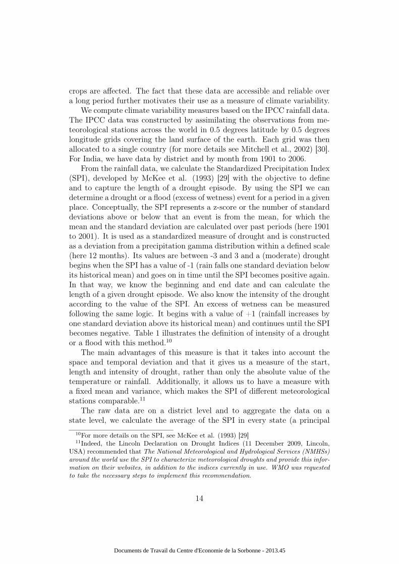
Table 1: Definitions of drought and flood according to the SPI

SPI values Category0 to -0.99 Mild drought-1 to -1.49 Moderate drought-1.5 to -1.99 Severe drought

<= -2 Extreme drought0 to 0.99 Mild flood1 to 1.49 Moderate flood1.5 to 1.99 Severe flood> = 2 Extreme flood

Source: McKee et al. (1993) [29] for drought and Guerreiro et al. (2008) [22] for flood.

component analysis is presented in Appendix A as a test of this procedure).We create five variables based on the SPI to measure the frequency, theduration and the magnitude of a drought or a flood:

1. Frequency : First, we define a binary variable by state which takesthe value of 1 if there was a drought/flood event in a month in thatstate, and 0 otherwise. The final measure is the number of monthswith drought/flood in the origin state during the five years precedingmigration.12 The measures count total months of either severe or mod-erate drought/flood. Extreme events are not common on the state leveldata. Aggregation at a state level takes out any extreme events at afiner district-level and may lead to less precise results.13

2. Maximal duration: In the aim to catch the impact of a long droughtor flood duration, we compute the maximal number of months that adrought/flood lasted in the five years preceding migration.

3. Magnitude: This variable is defined as the sum of the absolute valuesof the SPI for a drought or a flood five years preceding migration.

4. Average monthly magnitude: The magnitude divided by the frequency.12Barrios et al. (2006) [4], Naudé (2008) [34] and Strobl and Valfort (2012) [41] also use

a lag of five years for the impact of natural disasters and climate variables.13We would like to control for exogenous natural disasters other than climate-driven

ones (such as cyclones and other natural disasters), but the data we studied from EM-DAT, collected by the Centre for Research on the Epidemiology of Disasters (CRED), didnot seem reliable at the state level (as compared to the country level).

15


5. Longest drought/flood magnitude: The sum of the absolute values ofthe SPI of the longest drought or flood in the five years precedingmigration.

Our measures are strictly exogenous and not influenced by economic ac-tivity, in contrast to other environmental variables like soil degradation orair pollution.

4.4 Net State Domestic Product (NSDP)

The NSDP per capita is used as a measure of the income per capita of thestate. We use the database of the Reserve Bank of India and calculate thedeflated NSDP at constant price for the two years of interest (1990 and 2000).

The variable used is the ratio of the NSDP per capita of the destinationstate divided by that of the origin state, in the year preceding migration(t− 1), in order to reduce any endogeneity with the migration flows.

4.5 Distance between states

The distance between states (or countries in international studies) is com-monly used as a measure of migration costs, notably in those based upon thegravity model. We calculate the distance between different states, by takingthe most populated city as reference city, most often the capital of the state,but in some cases the economic center of the state, according to the greatcircle formula.14

dij = R ∗ cos−1(sin(a)sin(b) + cos(a)cos(b)cos(c− d)) (3)

where

dij: distance between state i and state jR: equatorial radius, equal to 6,378 kma: latitude degree of state ib: latitude degree of state jc: longitude degree of state id: longitude degree of state j

As explanatory variable we use the distance between two states, measuredin km.

14The latitudes and longitudes of the largest cities in every state can be found on thewebsite “Maps of India”. See www.mapsofindia.com

16


4.6 Common border and common language

We introduce a dummy variable to control for neighboring states. It takes thevalue of one for bilateral migration where the origin and destination stateshave a common border, and zero otherwise.

One of the specificities of India is that there are 18 different native lan-guages (English excluded) inside the country. As another proxy of the costof migration, we introduce a language dummy variable. It takes the valueof one for bilateral migration where the origin and destination states share acommon language, and zero otherwise. To assign a language to a state, wetook the major language spoken in the state. The source of this variable is“Maps of India”.

These two variables are proxies for cultural and traditional similaritiesbetween states.

4.7 Scheduled castes (SC) and scheduled tribes (ST)

In India, 16.2 % of the population belong to a scheduled caste (also called“the untouchables”) and 8.2% to scheduled tribes in 2001. In the literature ofIndian migration, these two factors are almost always taken into account toexamine the role of social factors in the migration decision.15 Indeed, theyplay an important role in Indian social structure. The “Hindu Varna” System,who establishes the classification of the society in India, excludes, categorizesand isolates groups of population, on the basis of the caste, the ethnicity andthe religion. This discrimination persists in the labour force participation(Dubey et al., 2006) [17]. In this social stratification, the SC and ST arethe most discriminated against and were the object of policies of positivediscrimination. The ST are isolated, partly because of their geographic loca-tions, often in hills and woods with weak density of population. But unlikethe SC, they had limitless access to the natural resources of land, water andforests where they live (Dubey et al., 2006) [17]. If these groups of individ-uals experience discrimination from upper castes and dominant groups, wemay hypothesize that they would like to stay within their communities andbe more likely to migrate (if they do so) where they can find their pairs.Indeed, Bhattacharya (2002) [9] find that scheduled castes are less likely tomigrate (from rural to urban areas) but if they do so, they go where they canfind other scheduled caste population. This suggests a social network effect.

We include the ratios of the scheduled caste and tribe rates in the desti-nation state compared to the origin state as another control for social simi-larities between states.

15See for example Bhattacharya (2002) [9] and Mitra and Murayama (2008) [31].

17


4.8 Descriptive statistics

Table 2 presents the mean, the standard deviation and the minimum andmaximum of each variable. The total number of observations is 1860, repre-senting bilateral migration flows across 31 Indian states in two years (1991and 2001).

The average of 8 migrants per 100,000 individuals may seem very small,but the variable measures the bilateral rate for a unique origin-destinationpair in one year. For example, 8 per 100,000 individuals migrate from Assamto West Bengal between 1990 and 1991, which represents a total of almost1800 individuals16. We have 930 possible combinations like this and we cananalyze an accumulated migration in a longer period than one year. It is alsoimportant to note that the dispersion is very large (the standard deviationis almost 4 times the mean) and that the bilateral migration rate can takevalues from 0 and up to 455 migrants per 100,000 individuals.

The average number of months (at any time) with a drought or floodevent is almost 15 months (out of a total of 5*12 months), but the descrip-tive statistics show large variation in the variable, as indeed for all climatevariability measures tested here. The longest duration of a drought over theperiod studied was on average 12 months, just as for a flood episode. Overthe time period studied the average drought and flood were of moderate size- an absolute value of the SPI of 0.81 for droughts and 0.83 for floods - buthigher for droughts than for floods in the sum of the absolute values of theSPI (16.42 compared to 15.15).

5 ResultsIn Table 3 we present six regressions with the PPML estimator. The sixregressions include origin state fixed effects and destination-time fixed ef-fects. Regression (1) is without the climate variability measures and in theregressions (2)-(6) the variables corresponding to drought events are includedone at a time. We introduce the five types of variables (drought frequency,longest drought duration, drought magnitude, average drought magnitudeper month, magnitude of the longest drought) separately because of the highcorrelation between them (see Table 9).

In all six regressions, the results show that the economic motivations,proxied by the ratio of the net state domestic product per capita betweenthe destination and the origin state are important, together with the variables

16There are 22,408,756 individuals that did not move in 1990 from West Bengal.

18


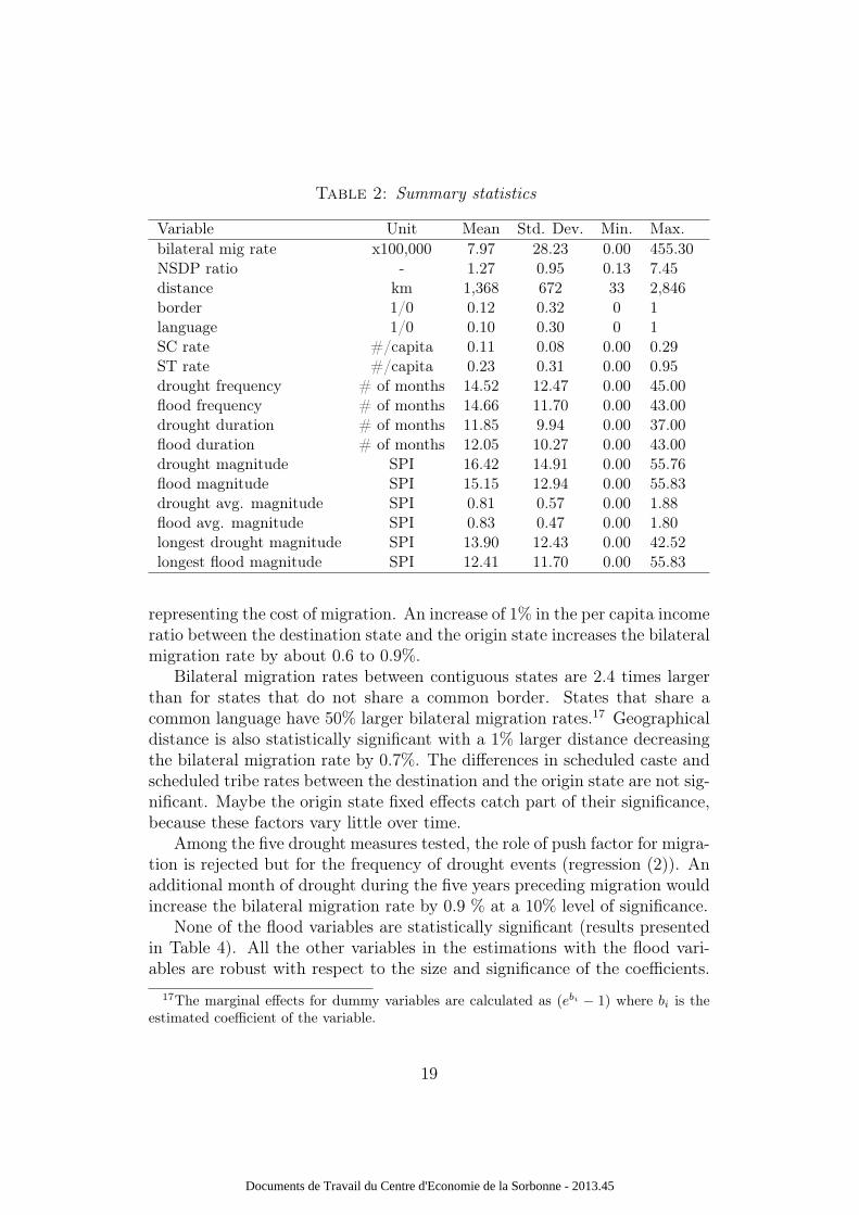
Table 2: Summary statistics

Variable Unit Mean Std. Dev. Min. Max.bilateral mig rate x100,000 7.97 28.23 0.00 455.30NSDP ratio - 1.27 0.95 0.13 7.45distance km 1,368 672 33 2,846border 1/0 0.12 0.32 0 1language 1/0 0.10 0.30 0 1SC rate #/capita 0.11 0.08 0.00 0.29ST rate #/capita 0.23 0.31 0.00 0.95drought frequency # of months 14.52 12.47 0.00 45.00flood frequency # of months 14.66 11.70 0.00 43.00drought duration # of months 11.85 9.94 0.00 37.00flood duration # of months 12.05 10.27 0.00 43.00drought magnitude SPI 16.42 14.91 0.00 55.76flood magnitude SPI 15.15 12.94 0.00 55.83drought avg. magnitude SPI 0.81 0.57 0.00 1.88flood avg. magnitude SPI 0.83 0.47 0.00 1.80longest drought magnitude SPI 13.90 12.43 0.00 42.52longest flood magnitude SPI 12.41 11.70 0.00 55.83

representing the cost of migration. An increase of 1% in the per capita incomeratio between the destination state and the origin state increases the bilateralmigration rate by about 0.6 to 0.9%.

Bilateral migration rates between contiguous states are 2.4 times largerthan for states that do not share a common border. States that share acommon language have 50% larger bilateral migration rates.17 Geographicaldistance is also statistically significant with a 1% larger distance decreasingthe bilateral migration rate by 0.7%. The differences in scheduled caste andscheduled tribe rates between the destination and the origin state are not sig-nificant. Maybe the origin state fixed effects catch part of their significance,because these factors vary little over time.

Among the five drought measures tested, the role of push factor for migra-tion is rejected but for the frequency of drought events (regression (2)). Anadditional month of drought during the five years preceding migration wouldincrease the bilateral migration rate by 0.9 % at a 10% level of significance.

None of the flood variables are statistically significant (results presentedin Table 4). All the other variables in the estimations with the flood vari-ables are robust with respect to the size and significance of the coefficients.

17The marginal effects for dummy variables are calculated as (ebi − 1) where bi is theestimated coefficient of the variable.

19


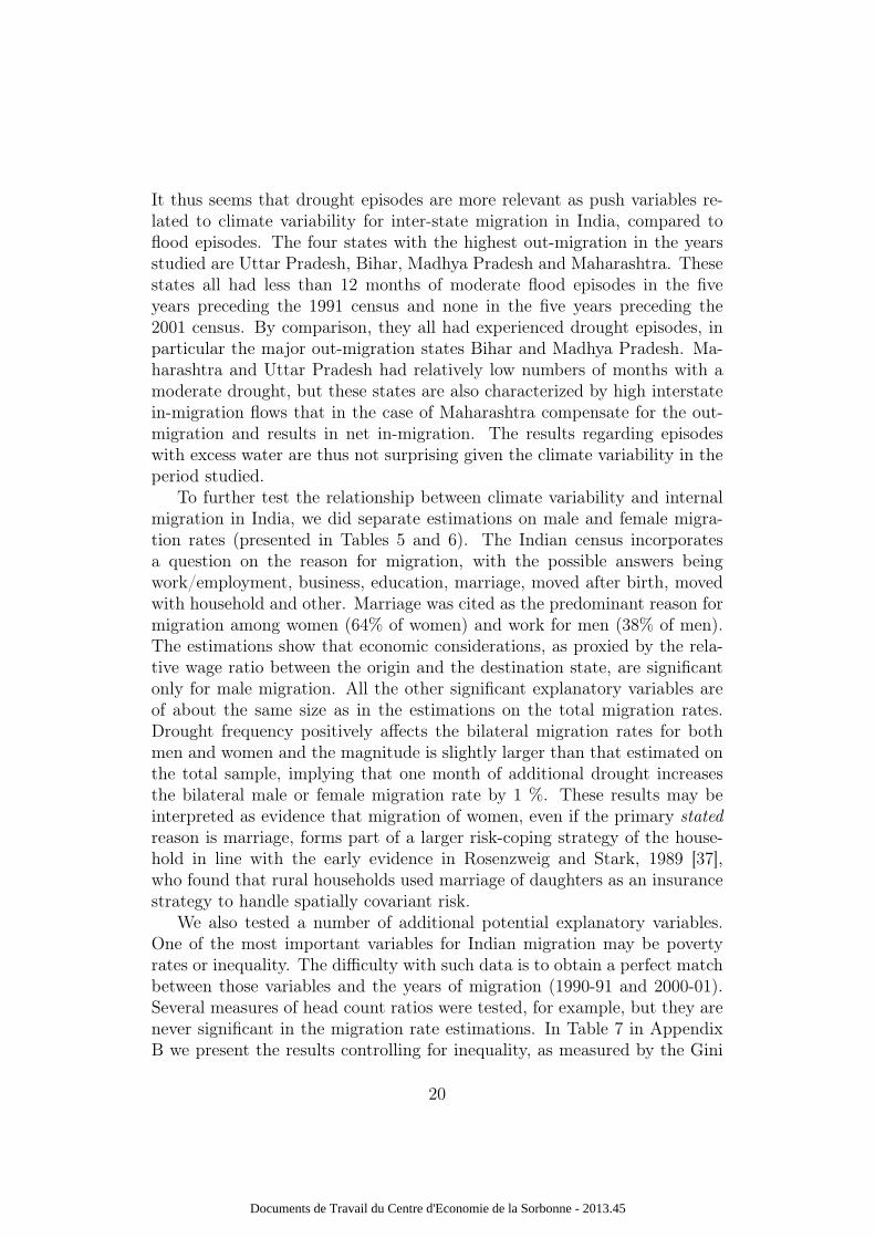
It thus seems that drought episodes are more relevant as push variables re-lated to climate variability for inter-state migration in India, compared toflood episodes. The four states with the highest out-migration in the yearsstudied are Uttar Pradesh, Bihar, Madhya Pradesh and Maharashtra. Thesestates all had less than 12 months of moderate flood episodes in the fiveyears preceding the 1991 census and none in the five years preceding the2001 census. By comparison, they all had experienced drought episodes, inparticular the major out-migration states Bihar and Madhya Pradesh. Ma-harashtra and Uttar Pradesh had relatively low numbers of months with amoderate drought, but these states are also characterized by high interstatein-migration flows that in the case of Maharashtra compensate for the out-migration and results in net in-migration. The results regarding episodeswith excess water are thus not surprising given the climate variability in theperiod studied.

To further test the relationship between climate variability and internalmigration in India, we did separate estimations on male and female migra-tion rates (presented in Tables 5 and 6). The Indian census incorporatesa question on the reason for migration, with the possible answers beingwork/employment, business, education, marriage, moved after birth, movedwith household and other. Marriage was cited as the predominant reason formigration among women (64% of women) and work for men (38% of men).The estimations show that economic considerations, as proxied by the rela-tive wage ratio between the origin and the destination state, are significantonly for male migration. All the other significant explanatory variables areof about the same size as in the estimations on the total migration rates.Drought frequency positively affects the bilateral migration rates for bothmen and women and the magnitude is slightly larger than that estimated onthe total sample, implying that one month of additional drought increasesthe bilateral male or female migration rate by 1 %. These results may beinterpreted as evidence that migration of women, even if the primary statedreason is marriage, forms part of a larger risk-coping strategy of the house-hold in line with the early evidence in Rosenzweig and Stark, 1989 [37],who found that rural households used marriage of daughters as an insurancestrategy to handle spatially covariant risk.

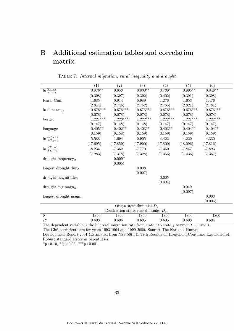
We also tested a number of additional potential explanatory variables.One of the most important variables for Indian migration may be povertyrates or inequality. The difficulty with such data is to obtain a perfect matchbetween those variables and the years of migration (1990-91 and 2000-01).Several measures of head count ratios were tested, for example, but they arenever significant in the migration rate estimations. In Table 7 in AppendixB we present the results controlling for inequality, as measured by the Gini

20


coefficient for rural areas of the origin state.18 The sign of the estimatedcoefficient is positive but never significant. The effect of a 1% increase inthe relative income ratio still varies between a 0.6 to 0.9% increase in thebilateral migration rate (although it is no longer significant in regression (2)).The impact of drought frequency is also robust.

As a final robustness test, we re-estimate the base specification (in Table3) removing one state at a time, to check whether the implicit assumptionof the econometric specification of independence of irrelevant alternatives isacceptable. In Table 8 we present the coefficients of the income ratio foreach of these 31 estimations. The income ratio is in all cases positive andsignificant, although somewhat lower in magnitude and at a lower level ofsignificance in the estimation where Uttar Pradesh was removed from thesample. The size of the impact of the income ratio remains around 0.6-0.9 otherwise, the major change occurring when the model is re-estimatedwithout Tamil Nadu - in this case the impact of the income ratio is higher(1.13). The test thus confirms the validity of the chosen specification.

18The majority of the internal migration flows in India are rural-rural (46%) or rural-urban (25%), compared to migration originating from urban areas.

21


Table 3: Internal migration and drought

(1) (2) (3) (4) (5) (6)ln

wj,t−1

wi,t−10.885** 0.652* 0.802** 0.741* 0.905** 0.852**(0.399) (0.396) (0.391) (0.402) (0.393) (0.398)

ln distanceij -0.676*** -0.676*** -0.676*** -0.676*** -0.676*** -0.676***(0.078) (0.078) (0.078) (0.078) (0.078) (0.078)

border 1.221*** 1.223*** 1.222*** 1.222*** 1.222*** 1.222***(0.147) (0.148) (0.148) (0.147) (0.147) (0.147)

language 0.404** 0.402** 0.403** 0.403** 0.404** 0.404**(0.160) (0.159) (0.159) (0.159) (0.159) (0.159)

lnSCjt+1SCit+1 0.484 -1.115 -2.209 0.558 -0.823 -0.202

(18.567) (18.727) (18.845) (18.625) (18.747) (18.708)ln

STjt+1STit+1 -7.118 -6.745 -7.113 -6.479 -6.742 -6.895

(6.691) (6.738) (6.734) (6.758) (6.808) (6.744)drought frequencyit 0.009*

(0.005)longest drought durit 0.008

(0.007)drought magnitudeit 0.005

(0.004)drought avg magnit 0.050

(0.096)longest drought magnit 0.003

(0.005)Origin state dummies Di

Destination state/year dummies Djt

N 1860 1860 1860 1860 1860 1860R2 0.692 0.696 0.695 0.694 0.692 0.693The dependent variable is the bilateral migration rate from state i to state j between t− 1 and t.Robust standard errors in parentheses.*p<0.10, **p<0.05, ***p<0.001

22


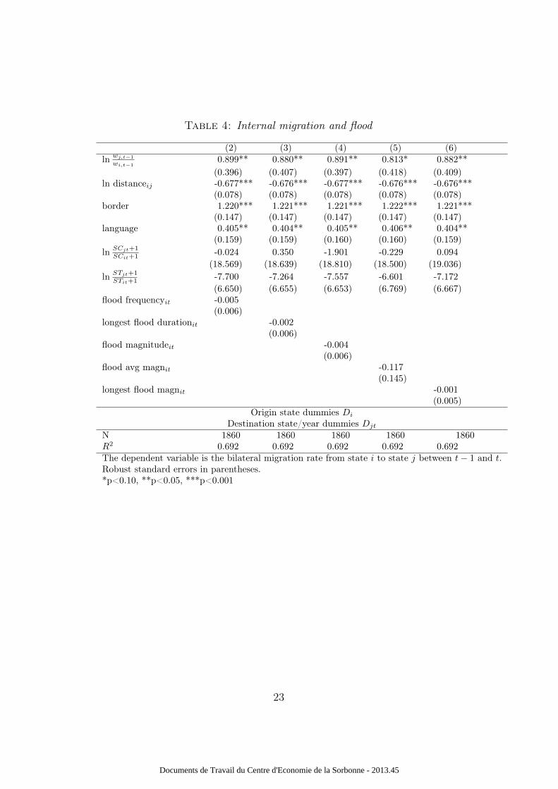
Table 4: Internal migration and flood

(2) (3) (4) (5) (6)ln

wj,t−1

wi,t−10.899** 0.880** 0.891** 0.813* 0.882**(0.396) (0.407) (0.397) (0.418) (0.409)

ln distanceij -0.677*** -0.676*** -0.677*** -0.676*** -0.676***(0.078) (0.078) (0.078) (0.078) (0.078)

border 1.220*** 1.221*** 1.221*** 1.222*** 1.221***(0.147) (0.147) (0.147) (0.147) (0.147)

language 0.405** 0.404** 0.405** 0.406** 0.404**(0.159) (0.159) (0.160) (0.160) (0.159)

lnSCjt+1SCit+1 -0.024 0.350 -1.901 -0.229 0.094

(18.569) (18.639) (18.810) (18.500) (19.036)ln

STjt+1STit+1 -7.700 -7.264 -7.557 -6.601 -7.172

(6.650) (6.655) (6.653) (6.769) (6.667)flood frequencyit -0.005

(0.006)longest flood durationit -0.002

(0.006)flood magnitudeit -0.004

(0.006)flood avg magnit -0.117

(0.145)longest flood magnit -0.001



N 1860 1860 1860 1860 1860R2 0.692 0.692 0.692 0.692 0.692The dependent variable is the bilateral migration rate from state i to state j between t− 1 and t.Robust standard errors in parentheses.*p<0.10, **p<0.05, ***p<0.001

23


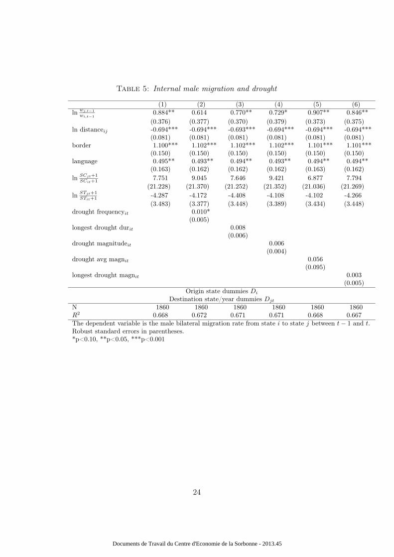
Table 5: Internal male migration and drought

(1) (2) (3) (4) (5) (6)ln

wj,t−1

wi,t−10.884** 0.614 0.770** 0.729* 0.907** 0.846**(0.376) (0.377) (0.370) (0.379) (0.373) (0.375)

ln distanceij -0.694*** -0.694*** -0.693*** -0.694*** -0.694*** -0.694***(0.081) (0.081) (0.081) (0.081) (0.081) (0.081)

border 1.100*** 1.102*** 1.102*** 1.102*** 1.101*** 1.101***(0.150) (0.150) (0.150) (0.150) (0.150) (0.150)

language 0.495** 0.493** 0.494** 0.493** 0.494** 0.494**(0.163) (0.162) (0.162) (0.162) (0.163) (0.162)

lnSCjt+1SCit+1 7.751 9.045 7.646 9.421 6.877 7.794

(21.228) (21.370) (21.252) (21.352) (21.036) (21.269)ln

STjt+1STit+1 -4.287 -4.172 -4.408 -4.108 -4.102 -4.266








N 1860 1860 1860 1860 1860 1860R2 0.668 0.672 0.671 0.671 0.668 0.667The dependent variable is the male bilateral migration rate from state i to state j between t− 1 and t.Robust standard errors in parentheses.*p<0.10, **p<0.05, ***p<0.001

24


Table 6: Internal female migration and drought

(1) (2) (3) (4) (5) (6)ln

wj,t−1

wi,t−10.508 0.295 0.447 0.372 0.582 0.484(0.415) (0.408) (0.402) (0.409) (0.404) (0.410)

ln distanceij -0.644*** -0.643*** -0.643*** -0.644*** -0.644*** -0.644***(0.078) (0.079) (0.078) (0.078) (0.078) (0.078)

border 1.381*** 1.384*** 1.383*** 1.382*** 1.381*** 1.382***(0.148) (0.149) (0.149) (0.148) (0.148) (0.148)

language 0.285* 0.284* 0.285* 0.284* 0.284* 0.285*(0.160) (0.160) (0.160) (0.160) (0.160) (0.160)

lnSCjt+1SCit+1 -6.085 -5.172 -6.282 -4.571 -8.499 -6.072

(15.554) (15.614) (15.568) (15.597) (15.474) (15.574)ln

STjt+1STit+1 -4.091 -4.748 -4.789 -4.379 -4.013 -4.385








N 1860 1860 1860 1860 1860 1860R2 0.718 0.721 0.720 0.720 0.718 0.719The dependent variable is the female bilateral migration rate from state i to state j between t− 1 and t.Robust standard errors in parentheses.*p<0.10, **p<0.05, ***p<0.001

25


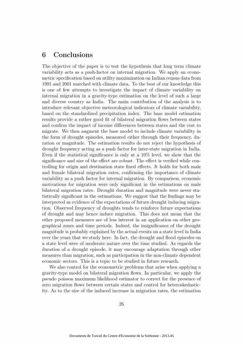
6 ConclusionsThe objective of the paper is to test the hypothesis that long term climatevariability acts as a push-factor on internal migration. We apply an econo-metric specification based on utility maximization on Indian census data from1991 and 2001 matched with climate data. To the best of our knowledge thisis one of few attempts to investigate the impact of climate variability oninternal migration in a gravity-type estimation on the level of such a largeand diverse country as India. The main contribution of the analysis is tointroduce relevant objective meteorological indicators of climate variability,based on the standardized precipitation index. The base model estimationresults provide a rather good fit of bilateral migration flows between statesand confirm the impact of income differences between states and the cost tomigrate. We then augment the base model to include climate variability inthe form of drought episodes, measured either through their frequency, du-ration or magnitude. The estimation results do not reject the hypothesis ofdrought frequency acting as a push factor for inter-state migration in India.Even if the statistical significance is only at a 10% level, we show that thesignificance and size of the effect are robust. The effect is verified while con-trolling for origin and destination state fixed effects. It holds for both maleand female bilateral migration rates, confirming the importance of climatevariability as a push factor for internal migration. By comparison, economicmotivations for migration were only significant in the estimations on malebilateral migration rates. Drought duration and magnitude were never sta-tistically significant in the estimations. We suggest that the findings may beinterpreted as evidence of the expectations of future drought inducing migra-tion. Observed frequency of droughts tends to reinforce future expectationsof drought and may hence induce migration. This does not mean that theother proposed measures are of less interest in an application on other geo-graphical zones and time periods. Indeed, the insignificance of the droughtmagnitude is probably explained by the actual events on a state level in Indiaover the years that we study here. In fact, the drought and flood episodes ona state level were of moderate nature over the time studied. As regards theduration of a drought episode, it may encourage adaptation through othermeasures than migration, such as participation in the non-climate dependenteconomic sectors. This is a topic to be studied in future research.

We also control for the econometric problems that arise when applying agravity-type model on bilateral migration flows. In particular, we apply thepseudo poisson maximum likelihood estimator to correct for the presence ofzero migration flows between certain states and control for heteroskedastic-ity. As to the size of the induced increase in migration rates, the estimation

26


results indicate that an additional month of drought in the origin state dur-ing the five years preceding migration increases the bilateral migration rateby 0.9%. Such an effect may seem small, especially when compared to theimportant role of barriers to migration in the Indian context that explainthe low Indian inter-state migration rates. Sharing a common language, forinstance, would increase the bilateral migration rate by 50 %. The impact ofdrought frequency is thus moderated by the barriers to migration. Neverthe-less, the results show that an increase in the frequency of drought events caninduce additional large numbers of inter-state migrants in absolute values.

Detailed analysis of the rainfall data shows that aggregation on the statelevel masks important variability between districts. A more detailed mod-elling of (rural-urban) migration flows at the district level thus seems appro-priate in order to further test the hypothesis that drought or flood episodesmay induce migration flows in excess of those normally observed. This is thesubject of ongoing research.

27


References[1] Anderson, J.E. (2011). The gravity model. Annual Review of Economics,

3, p. 133-160.

[2] Attri, S.D. & Tyagi, A. (2010). Climate profile of India. Government ofIndia Ministry of Earth Sciences India Meteorological Department. NewDelhi.

[3] Badiani, R. & Safir, A. (2010). Coping with aggregate shocks: Tem-porary migration and other labor responses to climatic shocks in ruralIndia. Mimeo World Bank.

[4] Barrios, S., Bertinelli L. & Strobl, E. A. (2006). Climatic change andrural-urban migration: The case of sub-Saharan Africa. Journal of Ur-ban Economics, 60(3), 357-371.

[5] Barrios, S., Bertinelli L. & Strobl, E. A. (2010). Trends in rainfall andeconomic growth in Africa: A neglected cause of the African growthtragedy. The Review of Economics and Statistics, 92(2), 350-366.

[6] Beine, M. & Parsons, C. (2012). Climate factors as determinants ofinternational migration. CESifo Working Papers No. 3747.

[7] Beine, M., Docquier, F. & Özden, C. (2011). Diasporas. Journal of De-velopment Economics, 95(1), 30-41.

[8] Bertoli, S. & Fernández-Huertas Moraga, J. (2013). Multilateral resis-tance to migration. Journal of Development Economics, forthcoming.

[9] Bhattacharya, P.C. (2002). Rural to urban migration in LDCS: a test oftwo rival models. Journal of International Development, 14(7), 951-972.

[10] Bhattacharya, H. & Innes, R. (2008). An empirical exploration of thepopulation-environment nexus in India. American Journal of Agricul-tural Economics, 90(4), 883-901.

[11] Bodvarsson, Ö. & Van den Berg, H. (2009). The economics of immigra-tion. Berlin Heidelberg: Springer-Verlag.

[12] Census of India (2011). Provisional Population Totals. Office of the Reg-istrar General and Census Commissioner, India. Paper 1 of 2011, IndiaSeries 1.

28


[13] Coniglio, N. & Pesce, G. (2011). Climate variability and internationalmigration: what are the links? Paper presented at the annual con-ference of the European Association of Environmental and ResourceEconomists, July 1, Rome.

[14] Datta, P. (2006). Urbanisation of India. Paper presented at The Regionaland Sub-Regional Population Dynamic - Population Process in UrbanAreas - European Population Conference, June 21-24, Liverpool.

[15] DeGaetano, A. T. (2001). Spatial grouping of United States climatestations using a hybrid clustering approach. International Journal ofClimatology, 21(7), 791-807.

[16] Dell, M., Jones, B.F. & Olken, B.A. (2009). Temperature and income:Reconciling new cross-sectional and panel estimates. American Eco-nomic Review, Papers and Proceedings 99(2), 198-204.

[17] Dubey, A., Palmer-Jones, R. & Sen, K. (2006). Surplus labour, socialstructure and rural to urban migration: Evidence from Indian data. TheEuropean Journal of Development Research, 18(1), 86-104.

[18] Feenstra, R.C. (2004). Advanced international trade: Theory and evi-dence. Princeton, NJ: Princeton University Press.

[19] The Government Office for Science, London (2011). Foresight: Migrationand Global Environmental Change, Final Project Report.

[20] Gray, C. (2009). Environment, land, and rural out-migration in theSouthern Ecuadorian Andes. World Development, 37(2), 457-468.

[21] Grogger, J. & Hanson, G.H. (2008). Income maximization and the se-lection and sorting of international migrants. NBER working paper No.13821.

[22] Guerreiro, M., Lajihna, T. & Abreu I. (2008). Flood analysis with thestandardized precipitation index. Revista da Faculdade de Ciencia e Tec-nologia de la Universidade Fernando Pessoa, 4, 8-14.

[23] Hornbeck, R. (2012). The enduring impact of the American Dust Bowl:Short and long-run adjustments to environmental catastrophe. AmericanEconomic Review, 102(4), 1477-1507.

[24] Karemera, D., Oguledo, V. & Davis, B. (2000). A gravity model analysisof international migration to North America. Applied Economics, 32(13),1745-1755.

29


[25] Lewer, J. & Van den Berg, H. (2008). A gravity model of immigration.Economics Letters, 99(1), 164-167.

[26] Marchiori, L. & Schumacher I. (2011). When nature rebels: interna-tional migration, climate change, and inequality. Journal of PopulationEconomics, 24(2), 569-600.

[27] Marchiori, L., Maystadt, J.-F. & Schumacher I. (2012). The impactof weather anomalies on migration in sub-Saharan Africa. Journal ofEnvironmental Economics and Management, 63, 355-374.

[28] Mayda, A. M. (2010). International migration : A panel data analysisof the determinants of bilateral flows. Journal of Population Economics,23(4), 1249-1274.

[29] McKee, T., Doesken, N. & Kleist, J. (1993). The relationship of droughtfrequency and duration to time scales. Paper presented at the 8th Con-ference on Applied Climatology, January 17-22, Anaheim, California,USA.

[30] Mitchell, T.D., Hulme, M. & New, M. (2002). Climate data for politicalareas. Area, 34(1), 109-112.

[31] Mitra, A. & Murayama, M. (2008). Rural to urban migration: A districtlevel analysis for India. IDE Discussion Paper. No. 137.

[32] Munoz-Diaz, D. & Rodrigo, F. (2004). Spatio-temporal patterns of sea-sonal rainfall in Spain (1912-2000) using cluster and principal componentanalysis: comparison. Annales Geophysicae, 22, 1435-1448.

[33] Myers, N. (1997). Environmental refugees. Population and Environment,19(2), 167-182.

[34] Naudé, W. (2008). Conflict, disasters, and no jobs : Reasons for interna-tional migration from Sub-Saharan Africa. United Nations University,Research Paper No. 2008/85.

[35] Özden, Ç. & Sewadeh, M. (2010). How important is migration?, In E.Ghani (Ed.) The poor half million in South Asia: What is holding backlagging regions? (pp. 294-322). New Delhi, India: Oxford UniversityPress.

[36] Reuveny, R. & Moore, W. (2009). Does environmental degradation in-fluence migration? Emigration to developed countries in the late 1980sand 1990s. Social Science Quarterly, 90(3), 461-479.

30


[37] Rosenzweig, M.R. & Stark, O. (1989). Consumption smoothing, mi-gration, and marriage: Evidence from rural India. Journal of PoliticalEconomy, 97(4), 905-926.

[38] Santos Silva, J.M.C. & Tenreyro, S. (2006). The log of gravity. TheReview of Economics and Statistics, 88(4), 641-658.

[39] Singh, K., & Singh, H. (1996). Space-time variation and regionalizationof seasonal and monthly summer monsoon rainfall of the sub-Himalayanregion and Gangetic plains of India. Climate Research, 6, 251-262.

[40] Stern, N. (2007). The economics of climate change: the Stern review.Cambridge: Cambridge University Press.

[41] Strobl, E.A. & Valfort, M. (2012). The effect of weather-induced in-ternal migration on local labor markets: Evidence from Uganda. IZADiscussion Paper No. 6923.

[42] Van Lottum, G. & Marks, D. (2010). The determinants of internal mi-gration in a developing country: Quantitative evidence for Indonesia,1930-2000. Applied Economics, 44(34), 4485-4494.

[43] Viswanathan, B. & Kumar, K.S.K. (2012). Weather variability, agri-culture and rural migration: Evidence from state and district level mi-gration in India. Paper presented at the 2nd International Conferenceon Environment and Natural Resources Management in Developing andTransition Economies (enrmdte), Clermont-Ferrand, October 17.

31


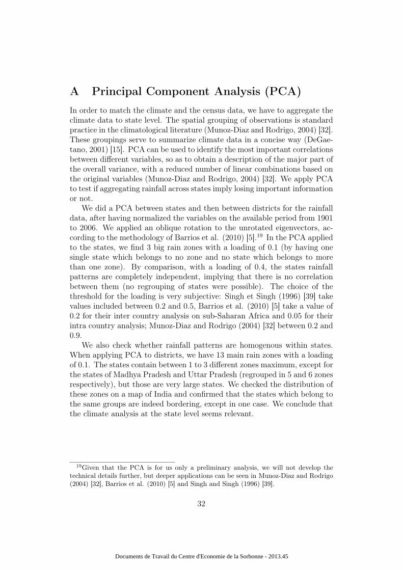
A Principal Component Analysis (PCA)In order to match the climate and the census data, we have to aggregate theclimate data to state level. The spatial grouping of observations is standardpractice in the climatological literature (Munoz-Diaz and Rodrigo, 2004) [32].These groupings serve to summarize climate data in a concise way (DeGae-tano, 2001) [15]. PCA can be used to identify the most important correlationsbetween different variables, so as to obtain a description of the major part ofthe overall variance, with a reduced number of linear combinations based onthe original variables (Munoz-Diaz and Rodrigo, 2004) [32]. We apply PCAto test if aggregating rainfall across states imply losing important informationor not.

We did a PCA between states and then between districts for the rainfalldata, after having normalized the variables on the available period from 1901to 2006. We applied an oblique rotation to the unrotated eigenvectors, ac-cording to the methodology of Barrios et al. (2010) [5].19 In the PCA appliedto the states, we find 3 big rain zones with a loading of 0.1 (by having onesingle state which belongs to no zone and no state which belongs to morethan one zone). By comparison, with a loading of 0.4, the states rainfallpatterns are completely independent, implying that there is no correlationbetween them (no regrouping of states were possible). The choice of thethreshold for the loading is very subjective: Singh et Singh (1996) [39] takevalues included between 0.2 and 0.5, Barrios et al. (2010) [5] take a value of0.2 for their inter country analysis on sub-Saharan Africa and 0.05 for theirintra country analysis; Munoz-Diaz and Rodrigo (2004) [32] between 0.2 and0.9.

We also check whether rainfall patterns are homogenous within states.When applying PCA to districts, we have 13 main rain zones with a loadingof 0.1. The states contain between 1 to 3 different zones maximum, except forthe states of Madhya Pradesh and Uttar Pradesh (regrouped in 5 and 6 zonesrespectively), but those are very large states. We checked the distribution ofthese zones on a map of India and confirmed that the states which belong tothe same groups are indeed bordering, except in one case. We conclude thatthe climate analysis at the state level seems relevant.

19Given that the PCA is for us only a preliminary analysis, we will not develop thetechnical details further, but deeper applications can be seen in Munoz-Diaz and Rodrigo(2004) [32], Barrios et al. (2010) [5] and Singh and Singh (1996) [39].

32


B Additional estimation tables and correlationmatrix

Table 7: Internal migration, rural inequality and drought

(1) (2) (3) (4) (5) (6)ln

wj,t−1

wi,t−10.876** 0.653 0.800** 0.739* 0.895** 0.846**(0.398) (0.397) (0.392) (0.402) (0.391) (0.398)

Rural Giniit 1.685 0.914 0.989 1.276 1.653 1.476(2.814) (2.746) (2.752) (2.765) (2.821) (2.781)

ln distanceij -0.676*** -0.676*** -0.676*** -0.676*** -0.676*** -0.676***(0.078) (0.078) (0.078) (0.078) (0.078) (0.078)

border 1.221*** 1.223*** 1.222*** 1.222*** 1.221*** 1.222***(0.147) (0.148) (0.148) (0.147) (0.147) (0.147)

language 0.405** 0.402** 0.403** 0.403** 0.404** 0.404**(0.159) (0.158) (0.159) (0.159) (0.159) (0.159)

lnSCjt+1SCit+1 5.588 1.694 0.905 4.422 4.220 4.330

(17.695) (17.859) (17.900) (17.800) (18.096) (17.816)ln

STjt+1STit+1 -8.234 -7.362 -7.770 -7.350 -7.847 -7.893








N 1860 1860 1860 1860 1860 1860R2 0.693 0.696 0.695 0.695 0.693 0.694The dependent variable is the bilateral migration rate from state i to state j between t− 1 and t.The Gini coefficients are for years 1993-1994 and 1999-2000. Source: The National HumanDevelopment Report 2001 (Estimated from NSS 50th & 55th Rounds on Household Consumer Expenditure).Robust standard errors in parentheses.*p<0.10, **p<0.05, ***p<0.001

33


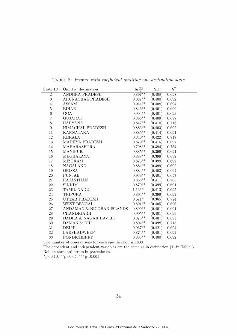
Table 8: Income ratio coefficient omitting one destination state

State ID Omitted destination lnwj

wiSE R2

2 ANDHRA PRADESH 0.897** (0.408) 0.6983 ARUNACHAL PRADESH 0.887** (0.400) 0.6924 ASSAM 0.944** (0.408) 0.6945 BIHAR 0.846** (0.401) 0.6996 GOA 0.904** (0.401) 0.6937 GUJARAT 0.866** (0.409) 0.6878 HARYANA 0.847** (0.410) 0.7169 HIMACHAL PRADESH 0.886** (0.403) 0.69211 KARNATAKA 0.885** (0.414) 0.69112 KERALA 0.840** (0.422) 0.71713 MADHYA PRADESH 0.879** (0.415) 0.69714 MAHARASHTRA 0.798** (0.394) 0.75415 MANIPUR 0.885** (0.399) 0.69116 MEGHALAYA 0.888** (0.399) 0.69217 MIZORAM 0.875** (0.399) 0.69218 NAGALAND 0.884** (0.399) 0.69219 ORISSA 0.884** (0.403) 0.69420 PUNJAB 0.938** (0.401) 0.65721 RAJASTHAN 0.858** (0.411) 0.70522 SIKKIM 0.879** (0.399) 0.69123 TAMIL NADU 1.13** (0.413) 0.69524 TRIPURA 0.894** (0.399) 0.69225 UTTAR PRADESH 0.671* (0.365) 0.72426 WEST BENGAL 0.891** (0.405) 0.69627 ANDAMAN & NICOBAR ISLANDS 0.899** (0.401) 0.69128 CHANDIGARH 0.905** (0.401) 0.69929 DADRA & NAGAR HAVELI 0.875** (0.401) 0.69330 DAMAN & DIU 0.894** (0.398) 0.71331 DELHI 0.967** (0.421) 0.69432 LAKSHADWEEP 0.874** (0.401) 0.69233 PONDICHERRY 0.885** (0.400) 0.692

The number of observations for each specification is 1800.The dependent and independent variables are the same as in estimation (1) in Table 3.Robust standard errors in parentheses.*p<0.10, **p<0.05, ***p<0.001

34


Tabl

e9:

Correlatio

nmatrix

(1)

(2)

(3)

(4)

(5)

(6)

(7)

(8)

(9)

(10)

(11)

(12)

(1)migration

rate

(2)NSD

Pratio

-0.091

5*(3)Rural

Ginir

atio

0.0093

-0.0807∗

(4)distan

ce-0.2778∗

-0.0060

-0.0124

(5)bo

rder

0.3589∗

-0.0257

0.0255

-0.5082∗

(6)lang

uage

0.2145∗

0.0022

-0.0447∗

-0.3970∗

0.2741∗

(7)SC

rate

0.0062

0.0918∗

0.3357∗

-0.1348∗

0.0884∗

0.0230

(8)ST

rate

-0.016

9-0.0299

-0.3876∗

0.0696∗

-0.0658∗

0.0678∗

-0.673

9∗

Dro

ught

vari

able

s(9)frequency

0.0047

0.0936∗

-0.0500∗

0.1018∗

-0.0426∗

0.0317

-0.288

4∗0.18

19∗

(10)

long

estdu

ration

-0.012

00.1252∗

-0.0568∗

0.0808∗

-0.0252

0.0154

-0.288

5∗0.18

75∗

0.95

26∗

(11)

magnitude

0.0161

0.0218

-0.0921∗

0.0980∗

-0.0463∗

0.0403∗

-0.310

7∗0.18

72∗

0.93

16∗

0.88

33∗

(12)

avg.

magn.

0.0153

-0.0615∗

-0.1113∗

0.0715∗

-0.0441∗

0.0169

-0.346

2∗0.18

97∗

0.65

37∗

0.66

77∗

0.78

19∗

(13)

long

estmagn.

0.0011

0.0335

-0.1184∗

0.0841∗

-0.0324

0.0269

-0.319

0∗0.19

47∗

0.88

88∗

0.90

49∗

0.97

13∗

0.81

31∗

Num

berof

observations:1860

∗p<

0.1

35
