Embed Size (px)
Citation preview
Centrality Analysisin
Vehicular Ad Hoc Networks
Technical Report
T-Labs/EPFL
August 28, 2008
Author : Yannick Do
Supervisors : Sonja Buchegger, Tansu Alpcan and Jean-Pierre Hubaux

Table of contents
1 Introduction 1
1.1 Project Goals . . . . . . . . . . . . . . . . . . . . . . . . . . . . . . . . . . . . . . 2
1.2 Contributions . . . . . . . . . . . . . . . . . . . . . . . . . . . . . . . . . . . . . . 2
1.3 Outline . . . . . . . . . . . . . . . . . . . . . . . . . . . . . . . . . . . . . . . . . 2
2 Related Work 5
2.1 Vanet Connectivity Analysis . . . . . . . . . . . . . . . . . . . . . . . . . . . . . . 5
2.2 Centrality Measures in Spatial Networks of Urban Streets . . . . . . . . . . . . . . 5
2.3 Social Network Analysis for Routing in Disconnected Delay-Tolerant MANETs . . . 6
3 System Model 7
3.1 Network . . . . . . . . . . . . . . . . . . . . . . . . . . . . . . . . . . . . . . . . 7
3.2 Mobility . . . . . . . . . . . . . . . . . . . . . . . . . . . . . . . . . . . . . . . . 10
3.3 Vehicular Infrastructure . . . . . . . . . . . . . . . . . . . . . . . . . . . . . . . . 11
3.4 Topology . . . . . . . . . . . . . . . . . . . . . . . . . . . . . . . . . . . . . . . . 13
4 Graph Theory & Centrality Analysis 15
4.1 Graph Theory . . . . . . . . . . . . . . . . . . . . . . . . . . . . . . . . . . . . . 15
4.2 Centrality Analysis . . . . . . . . . . . . . . . . . . . . . . . . . . . . . . . . . . . 16
4.2.1 Definition . . . . . . . . . . . . . . . . . . . . . . . . . . . . . . . . . . . 16
4.2.2 Measures . . . . . . . . . . . . . . . . . . . . . . . . . . . . . . . . . . . . 17
5 Experiments 23
5.1 Toolkit . . . . . . . . . . . . . . . . . . . . . . . . . . . . . . . . . . . . . . . . . 23
5.1.1 Datasets . . . . . . . . . . . . . . . . . . . . . . . . . . . . . . . . . . . . 23
5.2 Density and Centrality Localization (DCL) . . . . . . . . . . . . . . . . . . . . . . 24
5.2.1 GIS rural . . . . . . . . . . . . . . . . . . . . . . . . . . . . . . . . . . . . 25
5.2.2 GIS urban . . . . . . . . . . . . . . . . . . . . . . . . . . . . . . . . . . . 25
5.2.3 GIS city . . . . . . . . . . . . . . . . . . . . . . . . . . . . . . . . . . . . 25
5.2.4 others . . . . . . . . . . . . . . . . . . . . . . . . . . . . . . . . . . . . . 25
5.3 Multi-Hop Dissemination (MHD) . . . . . . . . . . . . . . . . . . . . . . . . . . . 27
5.4 Distance to Infrastructure Backbone (D2B) . . . . . . . . . . . . . . . . . . . . . . 30
6 Conclusions and Future Work 31
A DCL Results 33A.1 Rural setting . . . . . . . . . . . . . . . . . . . . . . . . . . . . . . . . . . . . . . 33A.2 Urban setting . . . . . . . . . . . . . . . . . . . . . . . . . . . . . . . . . . . . . . 37A.3 City setting . . . . . . . . . . . . . . . . . . . . . . . . . . . . . . . . . . . . . . . 39
B MHD Results 41B.1 Rural setting . . . . . . . . . . . . . . . . . . . . . . . . . . . . . . . . . . . . . . 41
B.1.1 noCF-noTL . . . . . . . . . . . . . . . . . . . . . . . . . . . . . . . . . . . 41B.1.2 CF-noTL . . . . . . . . . . . . . . . . . . . . . . . . . . . . . . . . . . . . 46B.1.3 CF-TL . . . . . . . . . . . . . . . . . . . . . . . . . . . . . . . . . . . . . 51
B.2 Urban setting . . . . . . . . . . . . . . . . . . . . . . . . . . . . . . . . . . . . . . 56B.2.1 noCF-noTL . . . . . . . . . . . . . . . . . . . . . . . . . . . . . . . . . . . 56B.2.2 CF-noTL . . . . . . . . . . . . . . . . . . . . . . . . . . . . . . . . . . . . 61B.2.3 CF-TL . . . . . . . . . . . . . . . . . . . . . . . . . . . . . . . . . . . . . 66
B.3 City setting . . . . . . . . . . . . . . . . . . . . . . . . . . . . . . . . . . . . . . . 67B.3.1 noCF-noTL . . . . . . . . . . . . . . . . . . . . . . . . . . . . . . . . . . . 67B.3.2 CF-noTL . . . . . . . . . . . . . . . . . . . . . . . . . . . . . . . . . . . . 68B.3.3 CF-TL . . . . . . . . . . . . . . . . . . . . . . . . . . . . . . . . . . . . . 69
C D2B Results 71C.1 Rural setting . . . . . . . . . . . . . . . . . . . . . . . . . . . . . . . . . . . . . . 71
C.1.1 noCF-noTL . . . . . . . . . . . . . . . . . . . . . . . . . . . . . . . . . . . 71C.1.2 CF-noTL . . . . . . . . . . . . . . . . . . . . . . . . . . . . . . . . . . . . 73C.1.3 CF-TL . . . . . . . . . . . . . . . . . . . . . . . . . . . . . . . . . . . . . 74
C.2 Urban setting . . . . . . . . . . . . . . . . . . . . . . . . . . . . . . . . . . . . . . 75C.2.1 noCF-noTL . . . . . . . . . . . . . . . . . . . . . . . . . . . . . . . . . . . 75C.2.2 CF-noTL . . . . . . . . . . . . . . . . . . . . . . . . . . . . . . . . . . . . 76C.2.3 CF-TL . . . . . . . . . . . . . . . . . . . . . . . . . . . . . . . . . . . . . 77
C.3 City setting . . . . . . . . . . . . . . . . . . . . . . . . . . . . . . . . . . . . . . . 78C.3.1 noCF-noTL . . . . . . . . . . . . . . . . . . . . . . . . . . . . . . . . . . . 78C.3.2 CF-noTL . . . . . . . . . . . . . . . . . . . . . . . . . . . . . . . . . . . . 79C.3.3 CF-TL . . . . . . . . . . . . . . . . . . . . . . . . . . . . . . . . . . . . . 80
Bibliography 81
Chapter 1Introduction
The number of casualties being in Europe or U.S. (40,000 deaths per year [1]) due to roadtraffic is still unacceptably high, even if it has reduced significantly over the years due to safervehicles, infrastructure and policies. Car ownership and use have continued to grow steadily,and the resulting congestion in built-up areas and on main highways has become a significantoverhead cost and burden for travelers, for the economy and for the environment. In VehicularAd Hoc networks (VANET), vehicles will be equipped with wireless short-range communica-tion devices, allowing vehicles and roadside infrastructure to communicate and form an Ad Hocnetwork.As it is envisioned, VANET raise both at the same time tremendous opportunities but also hugedesign challenges. VANET are thought as a way to enhance the use of vehicle transportationby providing many different kind of applications. For example safety and cooperative appli-cations, by periodic dissemination of information (position, speed, direction...). As well trafficefficiency could be increased. Hence by using communication and cooperation between vehiclescould significantly reduce the negative impacts of road traffic by creating additional effectiveroad network capacity and a more efficient use by vehicles.It remains that the big challenge comes in the deployment of this technology, specifically takinginto account the penetration of vehicular communication that will grow larger over the year. Away to bootstrap smoothly the technology and making coexist VANET enabled and non-enabledvehicles must be found. In that order of idea, study of Vehicular Infrastructure Integration VII,where the road environment is enhanced with sensing and communicating devices, is a first step.
Because it is not yet possible to rely on an omnipresent infrastructure, the network will relyon an hybrid solution consisting of vehicle-to-vehicle (V2V) and vehicle-to-infrastructure (V2I)communication. The latter should help enhancing the overall connectivity when V2V is notavailable and provide services among the network participants. Connectivity issues in VANEThave already been investigated [23][24], but there is still no clear understanding and consensuson how the vehicular infrastructure should be deployed efficiently. In this study we’ll focus ontopology and centrality analysis in order to asses how deployment of roadside infrastructure,Roadside UnitsRSUs, can affect connectivity in the network and which area can be consideredas hotspots.
What are the most efficient/hotspot points to deploy RSUs? Answers should take intoaccount different level of connectivity requirements. Characteristics of Delay-Tolerant-Networksis that at, any time, the network cannot safely assumed to be fully connected, and isolation ofnodes (vehicles) should be minimized.
2 Introduction
Why is it important? Improve network connectivity, data dissemination and protectionagainst attackers.
The originality of our approach is to use social networks metrics such as Centrality measures,both on traffic and on road topology. Social networks analysis approach focus on the idea thatsome places (streets, crossroads), actors (vehicles, roadside units) plays more important rolesthan others. By correlating Centrality both from a road and traffic topological point of view,we can have a new understanding of important regions in the network and use this knowledgeto deploy roadside infrastructure. A further step, would be to detect most vulnerable spots forattacker jamming. This would result in setting a game theoretic framework between attackerand authorities for battle of road safety.
1.1 Project Goals
Due to cost and technology adoption, the deployment of VANET is slow and yet still quiteexperimental. For a few years a lot of effort has been done in developing some real life testbed forvehicular networks. But to our knowledge the deployment of the infrastructure has not alwaysbeen the main point of interest. The infrastructure unit, RSU, can have many capabilities,such as sensing and broadcasting information. Up to now, it is a common understanding todeploy the RSU at major crossroads or at very dense area (such as highways). We believe thata characterization of the importance of a geographical region according to the road networkand car traffic flows is an alternative. Even though such a deployment seems to make sense,we believe that at the beginning of the infrastructure deployment, a smart placement of RSUcould perform as good as a dumb one and also have some advantages in economics terms (lessRSU) or flow control terms. Goals of the project are the following:
• Summarize centrality measures and their application in VANET.
• Compute density and centrality values for a road network based on realistic vehiculartraces.
• Define Road Side Units placement strategies.
1.2 Contributions
The quantification of some nodes importance is mainly a task in social network analysis.Here we try to adapt this research for Vehicular Networks thus providing a new approachin the field. Compared to classical Social networks graphs, Vehicular networks present someinteresting aspects. First of all due to the moving nature of the cars, network graphs arechanging frequently with the addition (or subtraction) of new relational ties between nodesthus we provide centrality measures data of interest.
1.3 Outline
This report is organized as follows:
Chapter 2 details the context where this project takes place and what relevant work hasalready been done.

1.3. Outline 3
Chapter 3 presents the system model and the assumptions of the project
Chapter 4 describes graph theory and centrality analysis by providing insight on a few met-rics.
Chapter 5 details the different experiments performed.
Chapter 6 concludes the project and gives some future directions.

4 Introduction
Chapter 2Related Work
First part of the work at T-Labs involved a large literature review on the global subject ofVehicular Ad-Hoc Networks and then on more specific themes such as Connectivity, VehicularInfrastructure Integration, Centrality and so on. Most of the papers read were summarized ina Google Notebook (ask author for access). In this chapter we present some of the work thatshowed to be the most relevant.
2.1 Vanet Connectivity Analysis
Kafsi et al. [24] is the result of the work of Mohamed Kafsi, a former colleague from EPFL,during his internship at T-Labs. In some way this project is the follow-up of his. VanetConnectivity Analysis describe relation between VANET connectivity, vehicles density, trafficflow, transmission range and market penetration. The main focus was put on the use ofpercolation theory. Therefore it heavily relies on the use of the SUMO Traffic Simulator [5].Unfortunately the topology and mobility model lacks real life element, with a N ×N grid mapand predefined traffic flows for different car densities. Even though it is a very simple andextensible setting, it probably cannot represent real life settings. That’s why in our project wechoose to use real traffic traces.The paper show that vehicle density is related too arrival flow but also too different mobilityregime, and that for high enough vehicle flows, density is stable in central parts and large inperipheral parts. The main contribution of this work is about the definition of connectivitywith respect too cluster size and vehicles density. Also the consideration of market penetrationshowed that background traffic can sometime affect positively connectivity level and moreprecisely the number of cars in the so-called biggest cluster.
2.2 Centrality Measures in Spatial Networks of Urban Streets
Crucitti et al. [17] is in some way the basic inspiration of our work. They investigated central-ity in urban street patterns and showed that spatial analysis allows an extended visualizationand characterization of a city structure. They used a primal approach which maps crossroadsto graph vertices and roads to graph edges. Dual approach is also possible, more details in[28]. They computed several centrality indices such as closeness, betweenness, straightness andinformation centrality and studied their distribution.
6 Related Work
2.3 Social Network Analysis for Routing in DisconnectedDelay-Tolerant MANETs
Even though we didn’t use much of the contribution of Daly and Haahr [18], it is a very in-teresting paper that show maybe the most effective use of social network and centrality analysisin mobile networking that is for routing. They use similarity and betweenness computation toderive a routing algorithm. Basic idea is that when message destination node is unknown tosource node, the message is forwarded to a more central node increasing the potential of findinga suitable carrier. Betweenness computation assuming reduction to ego network analysis (i.e.local centrality).
They come up with SimBet routing algorithm, which is close in performance with Epidemicrouting in terms of “total number of messages delivered”, “End-to-end delays” and “Averagenumber of hops” and this without the overhead of redundantly forwarding messages. Epidemicrouting is also outperformed when it comes to “total number of forward messages”.
Chapter 3System Model
In this chapter we discuss the system model adopted in this project. We first introduceVANET systems, describe their specificities and possible applications. As for any vehicularrelated project, we pay attention to the mobility models that are used. Then we speak aboutthe vehicular roadside infrastructure and what functions they provide and finish with a focuson the project topology.
3.1 Network
Vehicular Networks can be seen as a specific, and maybe the principal, application of Multi-Hop Mobile Ad Hoc Network. Main components are:
• Servers/Authorities: public agencies or corporations with administrative powers in aspecific field/region. They are responsible for instantiating procedures (e.g. registration,license issuance etc...) and managing security credentials.
• Roadside Units: act as base stations, can belong to governments or private serviceproviders.
• Public vehicle: public transportation (e.g. buses, taxi), public services (e.g. police).
• Private vehicle: belonging to individuals or private companies.
However there are some significant differences that make research on ad hoc network veryspecific.
Network dynamics characterized by VANET is quite different of classical MANET or sensornetworks. Quasi-permanent mobility, high speeds, and (in most cases) very short connectiontimes between communicating entities. Vehicles trajectories are mostly well defined by roads,which incurs advantages (message dissemination) and disadvantages (privacy). VANET isdefinitely the largest real-world application of mobile networks (100s millions of nodes), butcommunication remains mostly local (geographical) which make it partitionable and scalable.As opposed to usual ad-hoc networks, vehicles are enabled with advanced capabilities in termsof computing power, storage, and power management. Among all it posses secure positioningsystems. Similar to the “black box” of airplanes, vehicles will be equipped with Event DataRecorder for event reconstruction (e.g. in the case of accidents), front-end radars for detectingobstacles and environmental sensors.
8 System Model
Due to life-critical situations, real-time constraints and error tolerance can be very stringent.That’s why attacks on such networks can cause irremediable damages, and thus the needs ofstrong security requirements. Deployment of such networks is not expected before 2014, andpenetration of enabled-vehicles will be low at the beginning. Moreover Roadside infrastructuremight not be globally available because of cost issues.
Communication
Vehicles to Vehicles (V2V), Vehicles to Infrastructure (V2I) happens over the wireless radiomedium. Infrastructure to infrastructure happens via wired backbone network. In case of nodirect connectivity , Multi-Hop communication is used, where data is forwarded from one nodeto another, potentially via infrastructure, until it reaches it’s destination. When both are avail-able, V2V and V2I might exhibit significant difference in terms of communication, e.g. packetdelay, bandwidth consumption and packet loss [11].
For the sake of standardization, the Federal Communication Commission (FCC) has al-located a 75Mhz around the 5.9 GHz channel spectrum, the DSRC (Dedicated Short RangeCommunications) [2]. It is a short to medium range (up to 1000 meters) communicationsservice that supports both Public Safety and Private operations in roadside to vehicle and ve-hicle to vehicle communication environments. DSRC is meant to be a complement to cellularcommunications by providing very high data transfer rates (6-27Mbps) in circumstances whereminimizing latency in the communication link and isolating relatively small communicationzones are important. Around the world other 802.11-like technologies are also expected to bestandardize in this way. Beyond DSRC, vehicle networks can leverage on other wireless com-munication technologies, such as (licensed-frequency) existing 2.5/3G cellular networks, WiFi,broadband wireless (e.g. WiMax), infrared, or low-speed radio broadcast systems used todayfor traffic information [30].
Communication appends upon messages exchange between network actors. Messages canbe application specifics but for safety and traffic applications we derive 2 important types ofmessage:
• periodic message (beacons): obtain local traffic information, 1-hop broadcast.
• event-driven message (e.g. emergency message): information dissemination, possibly overMulti-Hop.
Those messages are mainly broadcast and standalone (i.e. there is no content dependencyamong them). Any safety and traffic related messages includes time-stamp, position, speed,direction, acceleration, and data-specific (e.g. congestion notification, accident). Upon receptionof messages, application On-board unit (OBU ) react accordingly (.e.g. if receive an accidentmessage, reduce speed,and change lane). Protocol design should ensure that messages areunique (non-replayable) and lifetime limited (area, TTL . . . ).
DSCR specifications say that safety messages can be transmitted over a single hop withsufficient power to warn vehicles in a range of 10-15 seconds travel time thus reducing need forMulti-Hop.
As proposed in [35], a possible and realistic protocol design is:
• Each vehicle sends beacons over a single hop every 300ms within a range of 10s (min110m max 300 m), other messages are sent upon triggered by event.
3.1. Network 9
• Inter message interval drops to 100ms (and the range to 15m) if the vehicle is very slowor stopped (i.e. their speed is less than 10 miles=16kmh).
• Vehicles take decision on the received messages and may transmit new ones.
• Safety messages can be discarded if the difference between sender and receiver time-stampis larger than a system-specific constant that accounts for the maximum clock drift andone-hop transmission, propagation and processing delays. Moreover messages can bediscarder at the receiver if the coordinates of its sender/relay, as reported in the message,indicate that the receiver is out of maximum radio range (validation on a per-hop manner)
Applications
VANET and Cooperative vehicle applications can be divided in three main categories:
1. Safety applications like accident warnings, warnings on environmental (e.g. ice on thepavement, aquaplaning etc), cooperative driving and collision avoidance. Because of thelife-critical situation, safety applications require strong security guarantees, very shorttiming constraints, and minimal isolation. The communication should mostly be local (afew km/ttl/hop at most). Require a very high penetration rate to be effective.
2. Traffic monitoring and optimization. Distributing the traffic as to minimize trafficjam and overall waiting time. For example, on apparition of traffic jam all incomingvehicles are rerouted to alternative shortest routes (avoid route mapping, see internetcongestion). Communication availability should be global (hundreds km) but timingconstraint are not life critical.
3. Infotainment-services applications like internet, video streaming, online payment andso on. Communication either local (payment at border for example) or global(internetaccess etc), but not time constrained. Business driven constraints could help deploymentof infrastructure.
A list of detailed applications is listed in [1]:
Optimum Traffic management Based on expected travel times and vehicle/driver destina-tion, it provide a personalized route planning to follow and to help the roadside manager topredict traffic congestion and delays.
Area routing Intersection controllers signal momentary disturbances in the traffic flow andgive individual, destination-based and appropriate routing alternatives to approaching vehicle.
Local Traffic Control Intersection optimization.
Flexible Lane Allocation To increase the capacity of the road infrastructure, a dedicatedbus lane is made available to “licensed” and CVIS-equipped vehicles, travelling in the samedirection, allowing them to use the lane when and where it would not be a nuisance to publictransport and the arguments of speed, punctuality and economy would not be compromised.
10 System Model
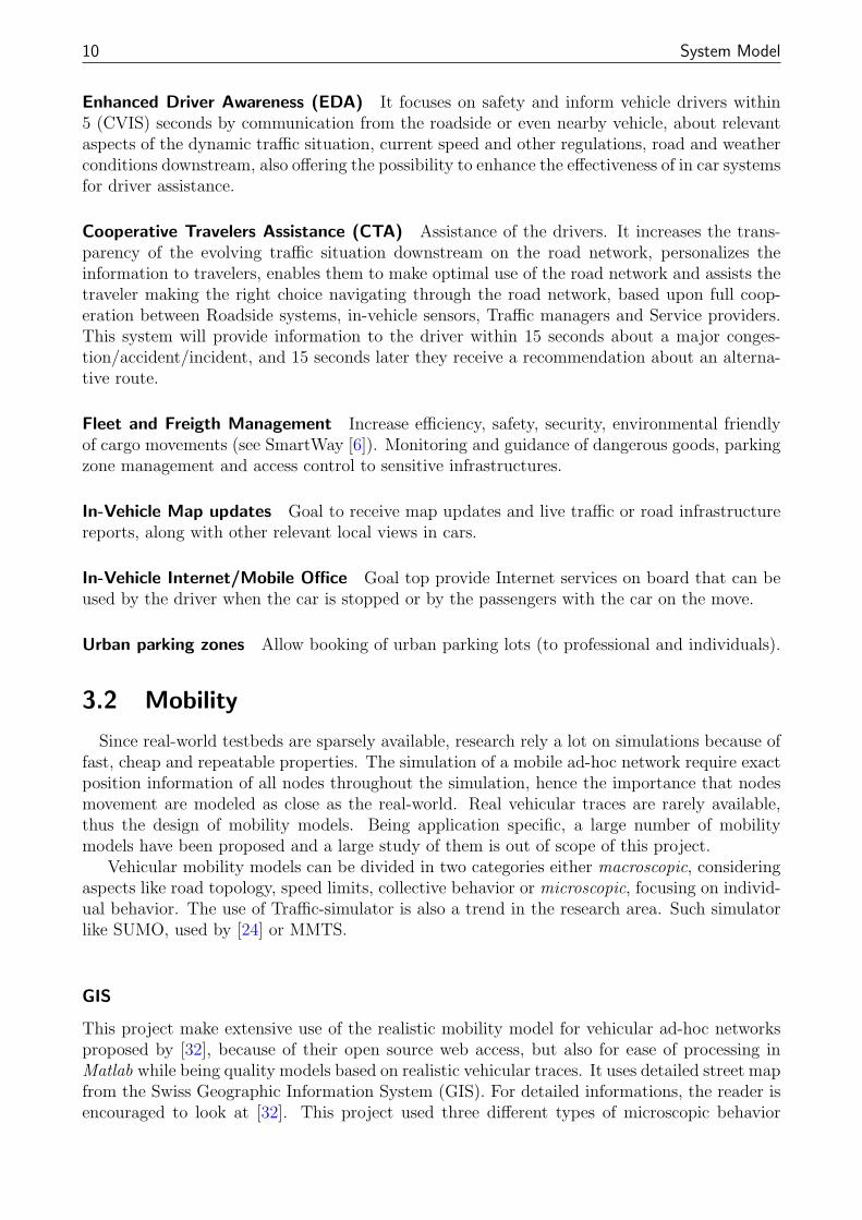
Enhanced Driver Awareness (EDA) It focuses on safety and inform vehicle drivers within5 (CVIS) seconds by communication from the roadside or even nearby vehicle, about relevantaspects of the dynamic traffic situation, current speed and other regulations, road and weatherconditions downstream, also offering the possibility to enhance the effectiveness of in car systemsfor driver assistance.
Cooperative Travelers Assistance (CTA) Assistance of the drivers. It increases the trans-parency of the evolving traffic situation downstream on the road network, personalizes theinformation to travelers, enables them to make optimal use of the road network and assists thetraveler making the right choice navigating through the road network, based upon full coop-eration between Roadside systems, in-vehicle sensors, Traffic managers and Service providers.This system will provide information to the driver within 15 seconds about a major conges-tion/accident/incident, and 15 seconds later they receive a recommendation about an alterna-tive route.
Fleet and Freigth Management Increase efficiency, safety, security, environmental friendlyof cargo movements (see SmartWay [6]). Monitoring and guidance of dangerous goods, parkingzone management and access control to sensitive infrastructures.
In-Vehicle Map updates Goal to receive map updates and live traffic or road infrastructurereports, along with other relevant local views in cars.
In-Vehicle Internet/Mobile Office Goal top provide Internet services on board that can beused by the driver when the car is stopped or by the passengers with the car on the move.
Urban parking zones Allow booking of urban parking lots (to professional and individuals).
3.2 Mobility
Since real-world testbeds are sparsely available, research rely a lot on simulations because offast, cheap and repeatable properties. The simulation of a mobile ad-hoc network require exactposition information of all nodes throughout the simulation, hence the importance that nodesmovement are modeled as close as the real-world. Real vehicular traces are rarely available,thus the design of mobility models. Being application specific, a large number of mobilitymodels have been proposed and a large study of them is out of scope of this project.
Vehicular mobility models can be divided in two categories either macroscopic, consideringaspects like road topology, speed limits, collective behavior or microscopic, focusing on individ-ual behavior. The use of Traffic-simulator is also a trend in the research area. Such simulatorlike SUMO, used by [24] or MMTS.
GIS
This project make extensive use of the realistic mobility model for vehicular ad-hoc networksproposed by [32], because of their open source web access, but also for ease of processing inMatlab while being quality models based on realistic vehicular traces. It uses detailed street mapfrom the Swiss Geographic Information System (GIS). For detailed informations, the reader isencouraged to look at [32]. This project used three different types of microscopic behavior
3.3. Vehicular Infrastructure 11
defining exact speed and acceleration of vehicles in the simulation: entity model, car-followingmodel, car-following with traffic light model.
Entity model The vehicle speed is imposed only by the road speed limit ignoring any othervehicles in proximity. Such a model is easily implemented but fails to reproduce realistic trafficeffects such as congestion.
Car-following model This model is based on Intelligent-Driver Model (IDM) [33]. The speedat next simulation step is a function of the current speed, a desired speed (aka road speedlimit), and distances to other vehicles.
Car-following model with traffic lights This is an extended version of the previous modeltaking into account intersections behavior. Upon arrival at intersections, foremost vehicle checkif it is free to pass. In the case of traffic light, the vehicle decelerates and stops. Since GIS mapsdo not reveal existence of traffic lights, [32] assume a first-come first-served principle on lessimportant intersections, and traffic lights on important intersections (round-robin algorithm).
MMTS
We also used vehicular traces from the Multi-Agent Microscopic Traffic Simulator (MMTS).These traces are realistic mobility traces for simulation of inter-vehicle networks obtained froma simulator that was developed by K. Nagel (at ETH Zurich, now at the Technical Universityin Berlin, Germany).
Nice properties of MMTS is the simulation of typical workday behavior. According to [10],individuals in the simulation are distributed over the cities and villages according to statisticaldata gathered by a census. Within the 24 hours of simulation, all individuals choose a timeto travel and the mean of transportation according to their needs and environment. E.g.,one individual might take a car and go to work in the early morning, another one wakes uplater and goes shopping using public transportation, etc. Travel plans are made based on roadcongestion; congestion in turn depends on the travel plans. To resolve this situation a standardrelaxation method is used.
The street network that is used in MMTS was originally developed for the Swiss regionalplanning authority (Bundesamt fur Raumentwicklung) and unfortunately the road detail levelis smaller than the one of [32]. [10] generated a 24 hour detailed car traffic trace file. The filecontains detailed simulation of the area in the canton of Zurich, this region includes the partwhere the main country highways connect to the city of Zurich, the largest city in Switzerland.Around 260’000 vehicles are involved in the simulation with more than 25’000’000 recordedvehicles direction/speed changes in an area of around 250km× 260km.
3.3 Vehicular Infrastructure
Roadside Units (RSU) aims at providing an increased connectivity between vehicles andservice provider. For example, when V2V communication is not available, or at specific hotspotsof network such as dense crossroads, dangerous curve etc... It is also a wide area gateway forCA/servers when they want for example to revoke some nodes credentials and/or make someinformation globally available (e.g. map update etc...).There is still no precise idea, or standard, on the topological deployment of those RSUs. Upon
12 System Model
literature review only some real-world testbed deployments exists, mainly in the US and Europe[8] [9] [31], their goal is to assess the feasibility of a global Vehicular Infrastructure Integration.
The market penetration will be low in the first few years, so a scalable and economicallyviable deployment of RSU is preferable. We believe that without deploying a large amount ofRSUs, efficiency would still be good.
In [24], a first step was to deploy RSU at crossroads mainly for cost motivations (trafficlights, electricity). It is also assumed a communication range identical as the one of a car. Stillthe finding is that the proportion of isolated cars (single node cluster) does not really changewhen introducing RSU at crossroads. This can be explain as such: when we have traffic lights,all cars at crossroad are in any case connected through each other (via Multi-Hop).
RSUs would help Safety applications by extending connectivity, but safety applications asdesigned should not be dependent of infrastructure presence because their scope is mainly localand safety messaging, as explained before, would be designed upon direct vehicle to vehiclecommunication. But in some case it can be useful, one example, is when a car has an accidentit trigger an event-message (emergency warning), upon receiving of this message other vehicleadapts their behavior and also might want to store and forward the message to closest RSU forhelp (call ambulance, police etc...). It could also rely on other technologies (cellular...) to callfor help. Problem with those safety application is that they require a high penetration rate.
In this project we want to compare scenarios with/without RSUs and different types ofRSU deployment. For this we need to find metrics to asses performance of the placement. Aninteresting one, would be the size of the area reachable in a 1-3 hop distance after emissionof a safety message for example. More generally, the shortest path lengths might be a goodindicator. Clustering coefficients tells us how close to a clique (fully interconnected) a graph orsubgraph is, so for high values of this coefficient, RSU would be of no use locally.
Goal of RSU:
• provide greater connectivity by minimizing isolated clusters (i.e. clusters that are notconnected to the vehicle infrastructure).
• gather traffic information
• be able to reach as many vehicles as possible
• provide shorter paths for information dissemination and hence less Multi-Hop.
We should note that some area of the networks might not necessarily need RSU coverage, it isa tradeoff between the efficiency to the network and the coast of the device.
RSU placements will be conditioned by the following measures:
1. density
2. cluster size
3. centrality
We can imagine two kind of infrastructure road side unit. The standard one where each RSUis interconnected to the infrastructure backbone, or a more lightweight and hence local one,static RSU which is not connected to the backbone infrastructure and who only act as a replayhence providing connectivity in a R range. Such local RSU could be parked cars.
Placing RSUs in the network graph is just about adding new “nodes”. If local RSUs, addnew 1-hop link (relay) between out-of-range nodes. If Global RSUs, add new paths betweenany pairs of nodes in source RSU area and sink RSU area. On a centrality analysis viewpoint
3.4. Topology 13
adding new paths can only shorten geodesics. For very distant pairs of nodes, it is likelythat geodesics goes through the RSUs backbone. Nodes on the old paths don’t belong to thegeodesics anymore hence their centrality decreases. Nodes around the RSUs are part of morenew geodesics hence their centrality increase. And of course RSU nodes get large centralityvalues.
Now it comes to define where to place those RSU. Let’s try to develop some placementstrategies and hypothesis:
Low Density Area (LD) + interconnect isolated cars (no more 1-cluster cars), + improveglobal connectivity (cars that could not communicate before can now), - impact uselessbecause only very few cars benefit of the service,
High Density Area (HD) + interconnect many very dense cluster (a lot of new connec-tions), - locally might be ineffective (cluster viewpoint) because since it is dense every carmight already have a path to any other, - Geodesics between any two nodes in differentclusters is likely to go through RSU, implying bottlenecks.
Low Centrality (LC) + balance centrality ( low central get more central, high central getless central)
High Centrality (HC) - high central get more central
Normalized High Centrality (HC N) Centrality/Density. Give more importance to areawhich have large centrality values, even for small time compared to area with relativelyslow values for long time.
Random (RD) +- random
3.4 Topology
We can consider two kind of topology: the network topology and the road topology.
Road topology First taking only topology, no traffic data, we can compute centrality for apice of map as done by [17]. We assume a road network map, represent crossroads as nodes androads as edges. We could compute centrality measures for each node (even edge). Edges weightvalues could be either geographical distance (and thus looking for shortest distance path), time-related (smallest accumulated time), or any combination. In order to analyze road topology, weneed a representation of the map such as with TIGER or even likely GIS (not sure). A parsermight be necessary to transform those data into graphs for computation of centrality metrics(See Future Work).
Network topology Vehicles and RSU are nodes, edges are between those nodes that arewithin radio range. With moving nodes, graph is subject to change frequently. Working withnetwork topology, and from the vehicular traffic traces of the mobility models in 3.2, we tryto extract informations. Centrality values can be derived by the knowledge at any time ofthe simulation of the tuple <Node_ID, timestamp, X_coord, Y_coord> and a fixed, binary,radio range (default is r = 300m), and thus we can take topology snapshots at specified timeintervals (default is 1s). We end up with a sequence of network graph 〈G1, . . . , GT 〉 on whichwe can compute some centrality metrics. We can also the development of an individuals metricover time.

14 System Model
Because we are not really interested in individual node value, we try to map back those valueto the road layer. Because of the knowledge of the <Node_ID, timestamp, X_coord, Y_coord>
tuple, this is easily done. For that mapping we need to divide the road map into areas. Wechoose to divide the map into squared grid blocks (default block size is b = 300m), but de-pending on the situation other choices can be suitable (e.g. segment in highway etc). Howthe mapping is done is also suitable to questions. We choose to sum centrality metrics at eachtimestep into the corresponding grid block at first. It would be interesting to compare centralitymetrics on road topology and network topology. Does it yield to same results?
Chapter 4Graph Theory & Centrality Analysis
The use of Centrality Analysis in Mobile Ad-Hoc Networks has seen very little attention fromthe research community [14], and in particular applications to VANET. Here we introduce whatwe believe to be relevant measures that can be used in VANET. First we refresh some knowledgeof graph theory and then introduce centrality analysis theory and present those measures.
4.1 Graph Theory
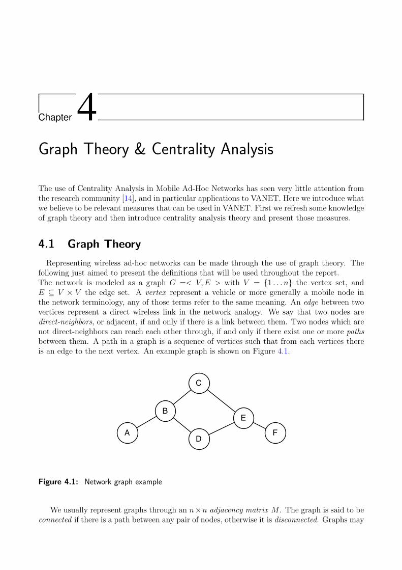
Representing wireless ad-hoc networks can be made through the use of graph theory. Thefollowing just aimed to present the definitions that will be used throughout the report.The network is modeled as a graph G =< V,E > with V = {1 . . . n} the vertex set, andE ⊆ V × V the edge set. A vertex represent a vehicle or more generally a mobile node inthe network terminology, any of those terms refer to the same meaning. An edge between twovertices represent a direct wireless link in the network analogy. We say that two nodes aredirect-neighbors, or adjacent, if and only if there is a link between them. Two nodes which arenot direct-neighbors can reach each other through, if and only if there exist one or more pathsbetween them. A path in a graph is a sequence of vertices such that from each vertices thereis an edge to the next vertex. An example graph is shown on Figure 4.1.
A
C
F
EB
D
Figure 4.1: Network graph example
We usually represent graphs through an n×n adjacency matrix M . The graph is said to beconnected if there is a path between any pair of nodes, otherwise it is disconnected. Graphs may
16 Graph Theory & Centrality Analysis
be undirected, meaning that there is no distinction between the two vertices associated witheach edge, or its edges may be directed from one vertex to another. The degree of a node ni in agraph G is the number of edges in G that have ni as endpoints. We speak about neighborhoodor k-neighborhood set of a node ni, as all nodes such that d(ni, nj) ≤ k hops .
4.2 Centrality Analysis
Social Networks Analysis is used to describe relation among individuals and groups. It makeuse of graph theory, mainly, in order to identify “most important” actors in a social network.This definition of importance has been a vast research field for more than 50 year and has yieldto the definition of many different metrics that measure properties of an actor location in asocial network. Interested readers about Social Networks Analysis should look towards [34].
This study focus on nondirectional relation (i.e. undirected graphs) for simplicity reason,assuming a two way directional communication between pair of nodes, but keeping in mind thatextension to directional relation (i.e directed graphs) is possible. Among the centrality metricsdiscussed, one can always look at the actor index which attempt to quantify the importanceof a single individual (node) in the network, or through aggregation of actors indices yieldinga group-level index in the goal to summarize how variable or differentiated the whole set ofactors is with respect to a given measure.
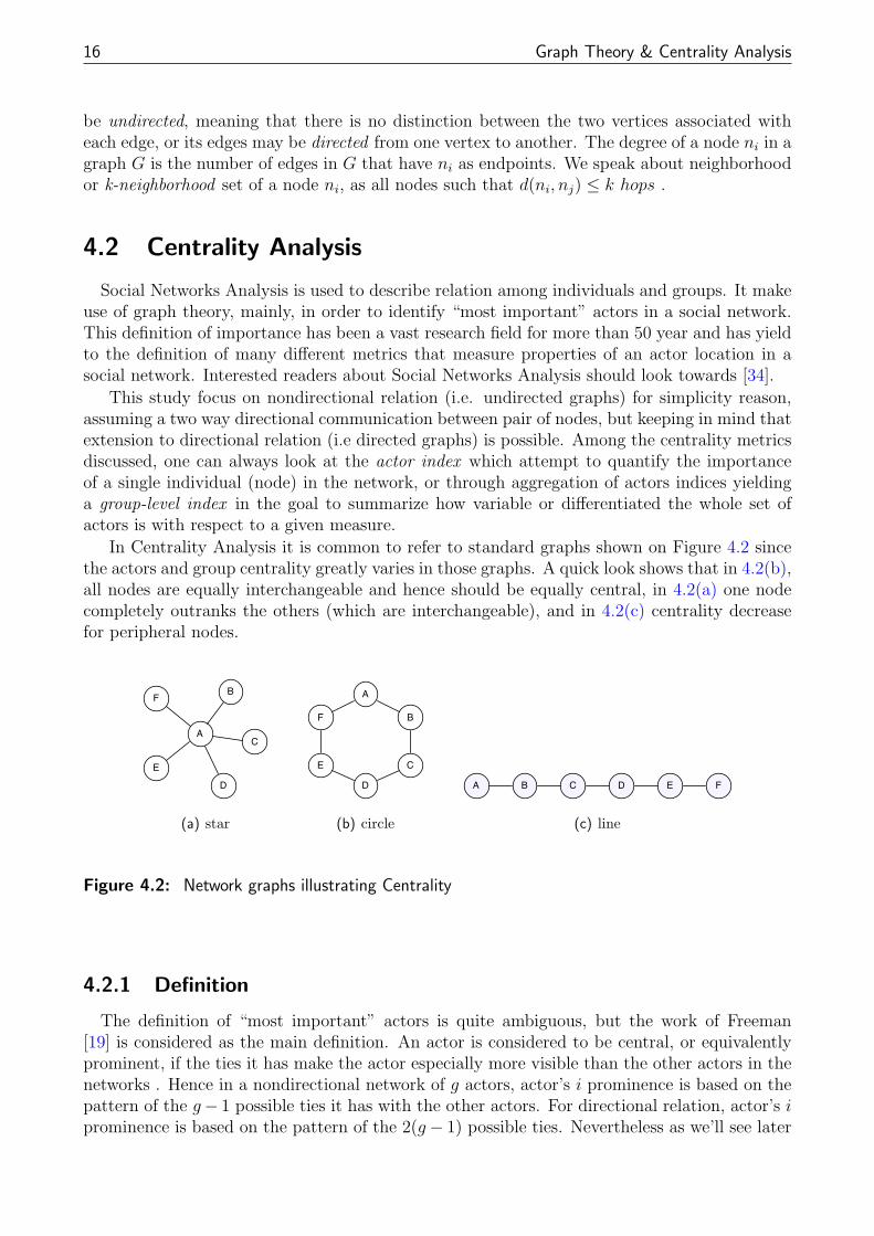
In Centrality Analysis it is common to refer to standard graphs shown on Figure 4.2 sincethe actors and group centrality greatly varies in those graphs. A quick look shows that in 4.2(b),all nodes are equally interchangeable and hence should be equally central, in 4.2(a) one nodecompletely outranks the others (which are interchangeable), and in 4.2(c) centrality decreasefor peripheral nodes.
AC
F
E
B
D
(a) star
A
C
F
E
B
D
(b) circle
A C FEB D
(c) line
Figure 4.2: Network graphs illustrating Centrality
4.2.1 Definition
The definition of “most important” actors is quite ambiguous, but the work of Freeman[19] is considered as the main definition. An actor is considered to be central, or equivalentlyprominent, if the ties it has make the actor especially more visible than the other actors in thenetworks . Hence in a nondirectional network of g actors, actor’s i prominence is based on thepattern of the g− 1 possible ties it has with the other actors. For directional relation, actor’s iprominence is based on the pattern of the 2(g− 1) possible ties. Nevertheless as we’ll see later
4.2. Centrality Analysis 17
on some specific definitions, it will also take into account choices made by intermediaries in thecentrality computation.
Actor Centrality Prominent actors are those that are extensively involved in relationshipswith other actors, being then more visible. Being the recipient or the source of the tie is nota concern, the actor being simply involved in the relation. So naturally the focus is first onnondirectional relations since there is no difference between source and recipient. Hence innondirectional relation, a central actor is one that is involved in many ties.
The work of [19] yield to the use of the casual notation when it come to actor centralitymeasures. C is a particular centrality measure, which will be a function of ni, where subscriptindex i range from 1 to g. As there is different version of centrality, C will be subscriptedwith an index for the particular measure under study. Then centrality measure A of node i isCA(ni).
Group Centralization Combining actors index in one group-level measure allow us to comparenetworks between each other. The group-level quantity is an index of centralization, and identifyhow variable or heterogenous the actors centralities are. It can also be seen as a measure of howunequal the network is. For example, the larger the group index is, the more likely there is onesingle very central actor in the network whereas other actors are considerably less central (forexample by being in the periphery of the network). Going back to the examples on Figure 4.2,star graph is maximally central because one central actor has ties with all other actors (whichdo not have any other ties). We define CA(n∗) = maxiCA(ni) as the largest value of indexA among all actors in the network. The general group centralization index, called Freeman’sindex, is:
CA =
∑gi=1[CA(n∗)− CA(ni)]
max∑g
i=1[CA(n∗)− CA(ni)]
where max∑g
i=1[CA(n∗) − CA(ni)] is the theoretical maximum possible sum of differences inactor centrality. This maximum being taken over all possible graphs of g actors. It can bedemonstrated, that this maximum occurs for the star graph. This Freeman’s index then leadsto quantity between 0 and 1. CA is 0 when all actors have equal centrality index, and is 1 ifone actor completely dominate the others (as in star graph).
4.2.2 Measures
Here we list the main measures of interest that are widely that can be used in networkanalysis.
Degree Centrality
Simplest definition of centrality is that central actors are the one that have the most ties inthe network graph, we say that there are the most active. Looking at the star graph, one nodehas g − 1 ties with all other actors, whereas the remaining have only 1 tie to the first actor.The first actor is the most active and hence maximally central. Circle graph has no actor moreactive than any other, so all have same centrality index. The Actor-degree centrality index isdefined as:
Actor Degree index:
CD(ni) = d(ni) =∑
j
xij =∑
i
xji
18 Graph Theory & Centrality Analysis
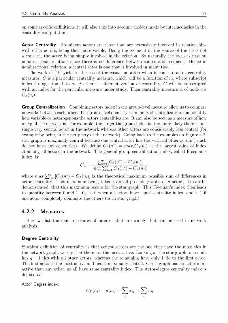
where xij = 1 if there is a link between nodes ni and nj. The measure is usually standardizedwith:
Standardized Actor Degree Index:
C ′D(ni) =d(ni)
g − 1
Actors with high level of centrality, measured by degree, should be recognized as where theaction is in the network. Thus this measure focus on the more visible actors in the network.According to the standard definition of group-level index, the group degree centralization indexis then:
Group Degree Centralization Index:
CD =
∑gi=1[CD(n∗)− CD(ni)]
max∑g
i=1[CD(n∗)− CD(ni)]=
∑gi=1[CD(n∗)− CD(ni)]
(g − 1)(g − 2)
It is 1 for star graph, and zero in a circle graph. There is also other indices based on degreesuch as graph density or variance of degrees [34].
Closeness Centrality
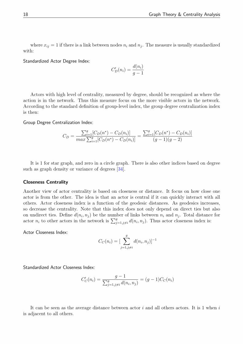
Another view of actor centrality is based on closeness or distance. It focus on how close oneactor is from the other. The idea is that an actor is central if it can quickly interact with allothers. Actor closeness index is a function of the geodesic distances. As geodesics increases,so decrease the centrality. Note that this index does not only depend on direct ties but alsoon undirect ties. Define d(ni, nj) be the number of links between ni and nj. Total distance foractor ni to other actors in the network is
∑gj=1,j 6=i d(ni, nj). Thus actor closeness index is:
Actor Closeness Index:
CC(ni) = [
g∑j=1,j 6=i
d(ni, nj)]−1
Standardized Actor Closeness Index:
C ′C(ni) =g − 1∑g
j=1,j 6=i d(ni, nj)= (g − 1)CC(ni)
It can be seen as the average distance between actor i and all others actors. It is 1 when iis adjacent to all others.

4.2. Centrality Analysis 19
Group Closeness Centralization Index:
CC =
∑gi=1[C
′C(n∗)− C ′C(ni)]
[(g − 2)(g − 1)/(2g − 3)]
The main drawback of this index is that it is only meaningful for a fully connected graph!In order to overcome this, [16] propose an interesting approach that circumvents the problemof disconnectedness. It offers the possibility to compute closeness centrality in both connectedand disconnected symmetric networks, and is based on the original Freeman’s index, but alsoincludes information about how an actor is not connected to others.
Betweenness Centrality
Betweenness centrality, in which most central nodes are the ones that are on many shortestpath of any nodes pair. It seems very suitable for investigation in VANET since wirelesscommunication tends to opt for shortest path, this could give us information about where doesthe communication flows. A fundamental assumption is that all geodesics (i.e. shortest paths)are equally likely to be used. The following Actor index are used:
Actor Betweenness index:
CB(ni) =∑
ns 6=nt 6=ni
gst(i)
gst
Standardized Actor Betweenness index:
C ′B(ni) =CB(ni)
(G− 1)(G− 2)
with gst number of geodesics linking node s and node t, gst(ni) number of geodesics linkingthe two actors that contains actor i, and G being the total number of actors G. Actor Between-ness index is an unbounded number whereas Standardized Actor Betweenness index range in[0, 1] with 1 when node is maximally central (e.g. middle node in a star graph) and 0 if it onno geodesics (e.g. edge node in star graph).In order to measure the centrality on the whole graph, we introduce:
Group Betweenness Centralization index:
CB =G∑
i=1
[C ′B(n∗)− C ′B(ni)]
(G− 1)
with CB(n∗) largest realized Actor Betweenness index for the set of actors. Group Be-tweenness index allow to compare different networks with respect to the heterogeneity of theBetweenness centrality of the members of different networks. Maximum value, unity, is reachedfor a star graph. Minimum value, zero, occurs when all actors have the same actor betweennessindex (e.g. a circle graph).
20 Graph Theory & Centrality Analysis
Others
Flow betweenness [26], as an alternative to classical betweenness, can also be another op-portunity if we assume, that communication does not travel through geodesic paths only. Thisindex can include non-geodesic path as well as geodesic paths. Path metrics can be in term ofdistance, time (speed limit, traffic free flow), or road segment utilization cost (e.g. toll).Information Centrality which relates the node centrality to the ability of the network torespond to its deactivation. For example, when looking at attacker possibilities if we are ableto build a network such that each node has as small as possible information centrality meaningthat no nodes is essential to the well behavior of the network. And thus under a jamming attack,the global efficiency of the network is not affected. Global efficiency [17], as the inverse averageshortest path length between any two nodes, is measure of how well the nodes communicatesover the network
Dynamic Networks & Temporal Betweenness Centrality
[22] propose methods to measure betweenness in time ordered networks. Focus on timing as-pects, introduction of betweenness with respect to temporal path, i.e.paths upon “aggregation”of snapshots. Importance of a node is not only on its position with respect to geodesics butalso at which time it appear on the geodesics.
Dynamic Network: series 〈G1, . . . , GT 〉 of static networks with Gt snapshot at time t. (G =(V,E), λ) is a dynamic network with λ time labeling function. Called multigraph.
Temporal paths: it is a (strict) time respecting path in the multigraph (i.e. time labels areincreasing).
Geodesics: length of the shortest temporal path. If there is no delays then d(u, v) is the num-ber of edges on the path p(u, v) otherwise it is the time difference of the first and lastinteraction d(u, v) = λ(vn−1, vn = v)− λ(v0 = u, v1) + 1.
Shortest Simple Temporal Path: ps(u, v) temporal paths with each individual present at mostonce and geodesics with delays.
Shortest Link path: pl(u, v) = min|ps(u, v)|.
Shortest Temporal Trails measure the ratio of time spent on an intermediate node to the totallength of the path. Same as Shortest Simple Temporal Path, but same individual canappear multiple time.
Betweenness: 1. Temporal Betweenness Centrality: importance of individuals based ontheir position in the shortest temporal path of all other nodes.
• gst number of shortest temporal path between s and t
• gst(v) number of shortest temporal path between s and t that pass through v.
• TBC of v is
BT (v) =∑
s 6=t6=v
BT (st)(v) =∑
s 6=t6=v
gst(v)
gst
2. Delay-Betweenness Centrality:
• nstst number of shortest trails from s to t.
• nstst(v) number of time steps of delay of v that all shortest trails from s to t.

4.2. Centrality Analysis 21
• DBC of v is
BD(v) =∑
s 6=t6=v
BD(st)(v) =∑
s 6=t6=v
nstst(v)
nstst

22 Graph Theory & Centrality Analysis

Chapter 5Experiments
Once we get hand on some vehicular traces of interest we aim at computing some centralityand connectivity related metrics
5.1 Toolkit
Being a follow up of the work of [24], we tried to push it too a more realistic analysis.Using SUMO [5] is nice to test some connectivity issues, and design experiments, our goal ofcomputing centrality measures can only be relevant for a realistic behavior of vehicles. That’swhy we did not pursue working with SUMO and preferred realistic traces. Vehicular traces aregenerated in NS2 format, hence allowing them to be later incorporated in tools such as TraNS,and in order to treat them with Matlab they need to be processed and sampled in order to geta matrix of position for each time step.
We used Matlab as a tool of choice in this project for the analysis of any mobility traces.Computation of centrality measures is not straightforward into Matlab, but the use of specificsocial network analysis tools such as UCINET [7] is not appropriate since they do not handlewell large sets (>500nodes), and we like to keep it simple into one single framework. Hopefully,the existence of Matlab Boost Graph Library [4], does a great job in helping to compute graphmetrics and extend our toolkit with nice graph theoretic features. Moreover it provide theability to compute betweenness centrality in a very efficient way.
If you are interested in the Matlab Toolkit or centrality data just ask me.
5.1.1 Datasets
GMSF
Generic Mobility Simulation Framework (GMSF) from [32] is a mobility traces online generator(http://polar9.ethz.ch/gmsf/).The choice of the following parameters is possible:
• Mobility Model: GIS, MMTS, Manhattan (not used) and Random Waypoint (not used)
• Scenario: rural, urban, city
• Number of Nodes
24 Experiments
• Simulation Time
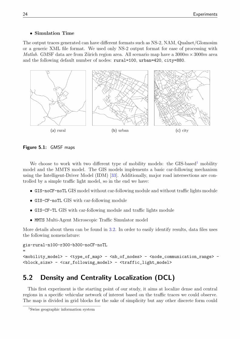
The output traces generated can have different formats such as NS-2, NAM, Qualnet/Glomosimor a generic XML file format. We used only NS-2 output format for ease of processing withMatlab. GMSF data are from Zurich region area. All scenario map have a 3000m×3000m areaand the following default number of nodes: rural=100, urban=420, city=880.
(a) rural (b) urban (c) city
Figure 5.1: GMSF maps
We choose to work with two different type of mobility models: the GIS-based1 mobilitymodel and the MMTS model. The GIS models implements a basic car-following mechanismusing the Intelligent-Driver Model (IDM) [33]. Additionally, major road intersections are con-trolled by a simple traffic light model, so in the end we have:
• GIS-noCF-noTL GIS model without car-following module and without traffic lights module
• GIS-CF-noTL GIS with car-following module
• GIS-CF-TL GIS with car-following module and traffic lights module
• MMTS Multi-Agent Microscopic Traffic Simulator model
More details about them can be found in 3.2. In order to easily identify results, data files usesthe following nomenclature:
gis-rural-n100-r300-b300-noCF-noTL
=
<mobility_model> - <type_of_map> - <nb_of_nodes> - <node_communication_range> -
<block_size> - <car_following_model> - <traffic_light_model>
5.2 Density and Centrality Localization (DCL)
This first experiment is the starting point of our study, it aims at localize dense and centralregions in a specific vehicular network of interest based on the traffic traces we could observe.The map is divided in grid blocks for the sake of simplicity but any other discrete form could
1Swiss geographic information system
5.2. Density and Centrality Localization (DCL) 25
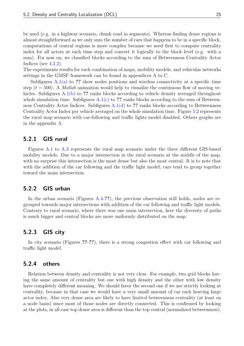
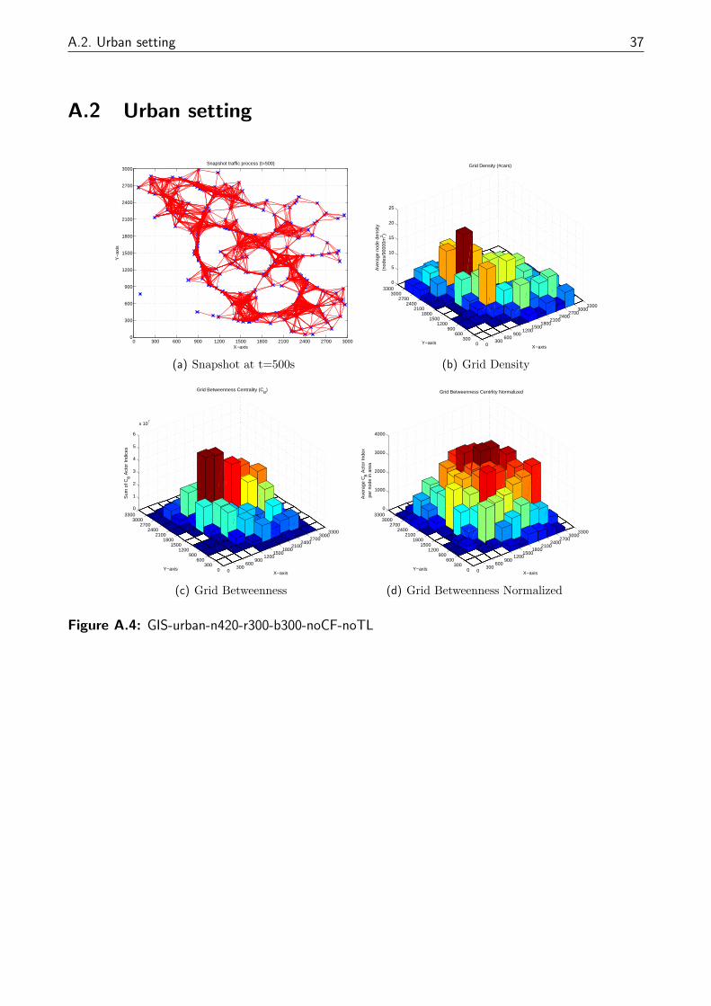
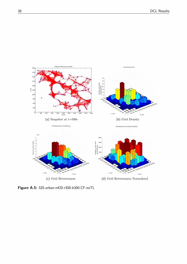
be used (e.g. in a highway scenario, chunk road in segments). Whereas finding dense regions isalmost straightforward as we only sum the number of cars that happens to be in a specific block,computations of central regions is more complex because we need first to compute centralityindex for all actors at each time step and convert it logically to the block level (e.g. with asum). For now on, we classified blocks according to the sum of Betweenness Centrality ActorIndices (see 4.2.2).The experiments results for each combination of maps, mobility models, and vehicular networkssettings in the GMSF framework can be found in appendices A to C.
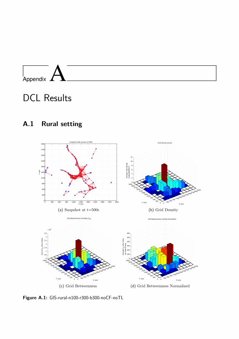
Subfigures A.1(a) to ?? show nodes positions and wireless connectivity at a specific timestep (t = 500). A Matlab animation would help to visualize the continuous flow of moving ve-hicles. Subfigures A.1(b) to ?? ranks blocks according to vehicle density averaged throughoutwhole simulation time. Subfigures A.1(c) to ?? ranks blocks according to the sum of Between-ness Centrality Actor Indices. Subfigures A.1(d) to ?? ranks blocks according to BetweennessCentrality Actor Index per vehicle averaged on the whole simulation time. Figure 5.2 representsthe rural map scenario with car-following and traffic lights model disabled. Others graphs arein the appendix A.
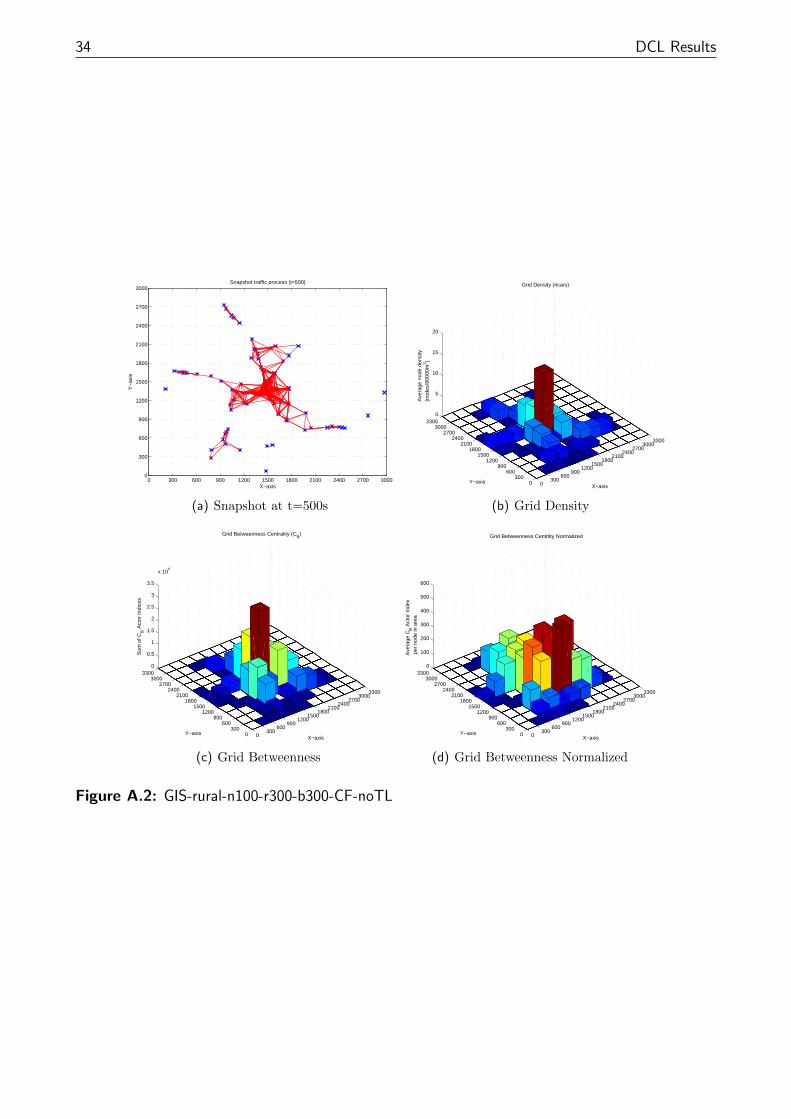
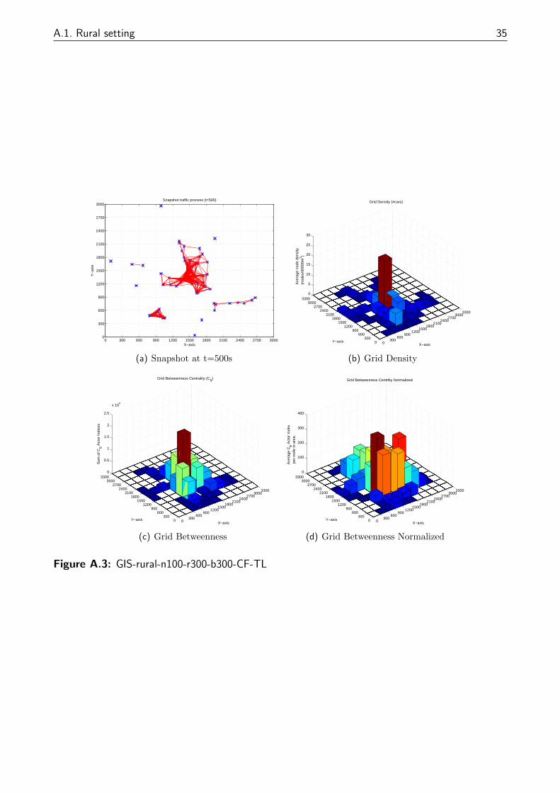
5.2.1 GIS rural
Figures A.1 to A.3 represents the rural map scenario under the three different GIS-basedmobility models. Due to a major intersection in the rural scenario at the middle of the map,with no surprise this intersection is the most dense but also the most central. It is to note thatwith the addition of the car following and the traffic light model, cars tend to group togethertoward the main intersection.
5.2.2 GIS urban
In the urban scenario (Figures A.4-??), the previous observation still holds, nodes are re-grouped towards major intersections with addition of the car following and traffic light models.Contrary to rural scenario, where there was one main intersection, here the diversity of pathsis much bigger and central blocks are more uniformly distributed on the map.
5.2.3 GIS city
In city scenario (Figures ??-??), there is a strong congestion effect with car following andtraffic light model.
5.2.4 others
Relation between density and centrality is not very clear. For example, two grid blocks hav-ing the same amount of centrality but one with high density and the other with low densityhave completely different meaning. We should favor the second one if we are strictly looking atcentrality, because in that case we would have a very small amount of car each heaving largeactor index. Also very dense area are likely to have limited betweenness centrality (at least ona node basis) since most of those nodes are directly connected. This is confirmed by lookingat the plots, in all case top dense area is different than the top central (normalized betweenness).
26 Experiments
0 300 600 900 1200 1500 1800 2100 2400 2700 30000
300
600
900
1200
1500
1800
2100
2400
2700
3000Snapshot traffic process (t=500)
X−axis
Y−
axis
(a) Snapshot at t=500s
0300
600900
12001500
18002100
24002700
30003300
0300
600900
12001500
18002100
24002700
30003300
0
2
4
6
8
10
12
X−axis
Grid Density (#cars)
Y−axis
Ave
rage
nod
e de
nsity
(n
odes
/900
00m
2 )
(b) Grid Density
0300
600900
12001500
18002100
24002700
30003300
0300
600900
12001500
18002100
24002700
30003300
0
0.5
1
1.5
2
2.5
3
3.5
x 106
X−axis
Grid Betweenness Centrality (CB)
Y−axis
Sum
of C
B A
ctor
Indi
ces
(c) Grid Betweenness
0300
600900
12001500
18002100
24002700
30003300
0300
600900
12001500
18002100
24002700
30003300
0
100
200
300
400
500
600
X−axis
Grid Betweenness Centrlity Normalized
Y−axis
Ave
rage
CB A
ctor
Inde
x p
er n
ode
in a
rea
(d) Grid Betweenness Normalized
Figure 5.2: GIS-rural-n100-r300-b300-noCF-noTL
5.3. Multi-Hop Dissemination (MHD) 27
If we look at the Normalized Betweenness subfigures (A.1(d)-A.3(d) and A.4(d)-??), in bothrural and urban scenario, the behavior is interesting. The centrality per vehicle is also moreuniformly distributed on the whole map.
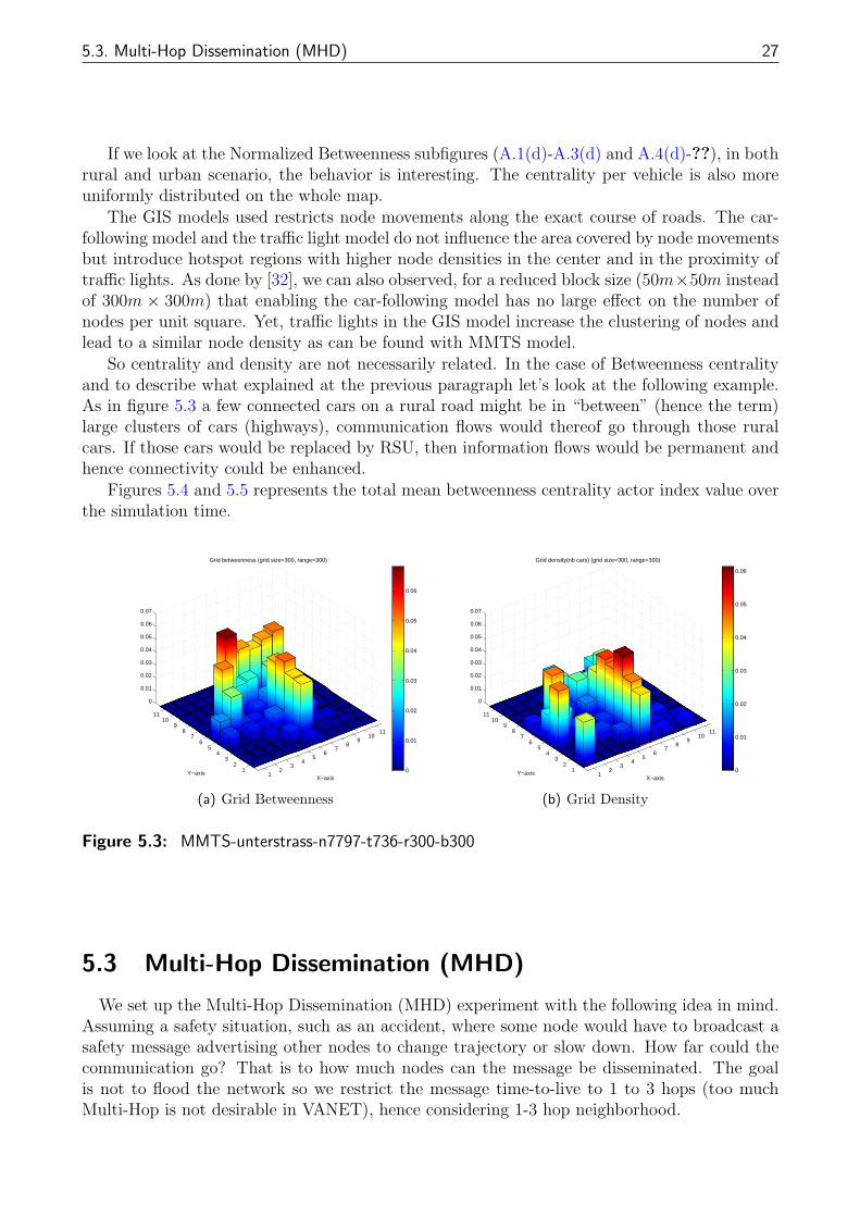
The GIS models used restricts node movements along the exact course of roads. The car-following model and the traffic light model do not influence the area covered by node movementsbut introduce hotspot regions with higher node densities in the center and in the proximity oftraffic lights. As done by [32], we can also observed, for a reduced block size (50m×50m insteadof 300m × 300m) that enabling the car-following model has no large effect on the number ofnodes per unit square. Yet, traffic lights in the GIS model increase the clustering of nodes andlead to a similar node density as can be found with MMTS model.
So centrality and density are not necessarily related. In the case of Betweenness centralityand to describe what explained at the previous paragraph let’s look at the following example.As in figure 5.3 a few connected cars on a rural road might be in “between” (hence the term)large clusters of cars (highways), communication flows would thereof go through those ruralcars. If those cars would be replaced by RSU, then information flows would be permanent andhence connectivity could be enhanced.
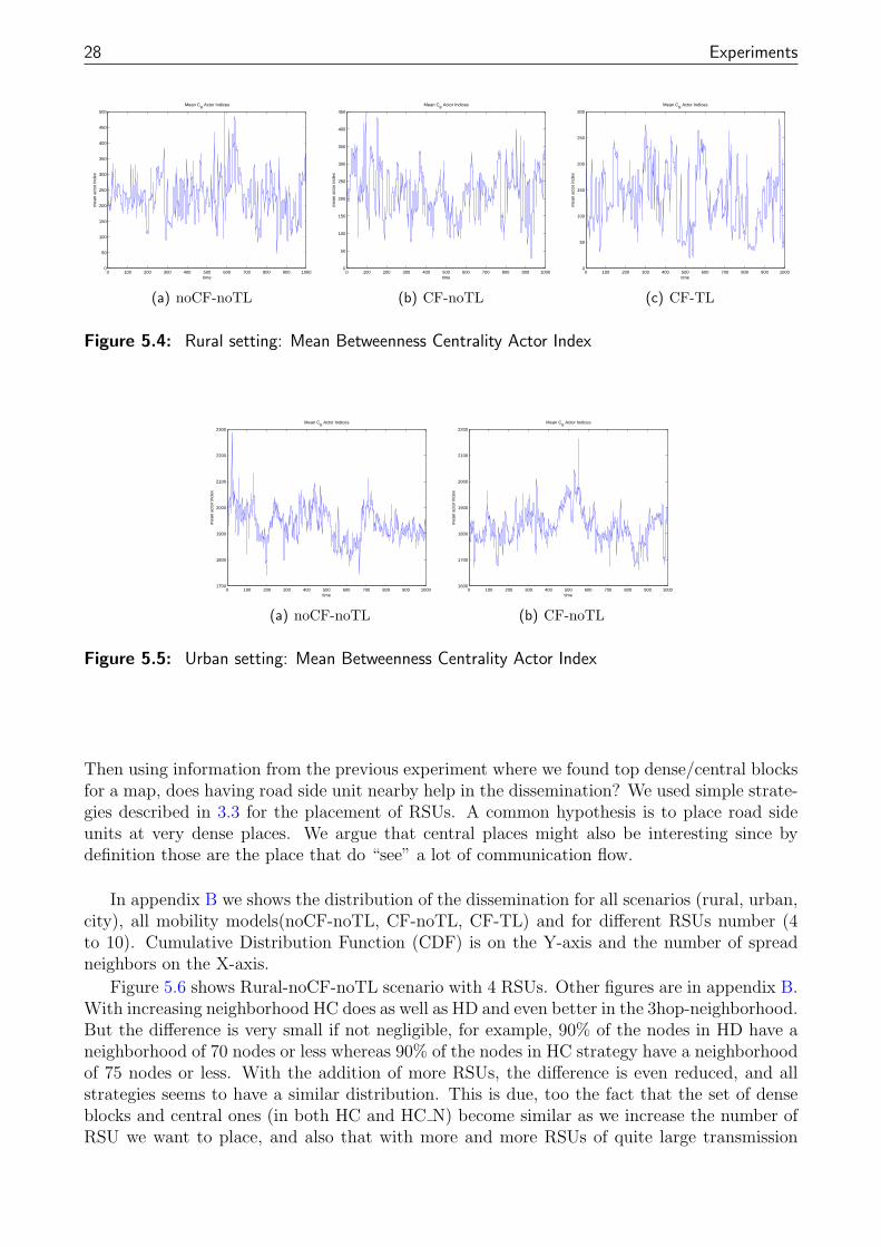
Figures 5.4 and 5.5 represents the total mean betweenness centrality actor index value overthe simulation time.
12
34
56
78
910
11
12
34
56
78
910
11
0
0.01
0.02
0.03
0.04
0.05
0.06
0.07
X−axis
Grid betweenness (grid size=300, range=300)
Y−axis 0
0.01
0.02
0.03
0.04
0.05
0.06
(a) Grid Betweenness
12
34
56
78
910
11
12
34
56
78
910
11
0
0.01
0.02
0.03
0.04
0.05
0.06
0.07
X−axis
Grid density(nb cars) (grid size=300, range=300)
Y−axis 0
0.01
0.02
0.03
0.04
0.05
0.06
(b) Grid Density
Figure 5.3: MMTS-unterstrass-n7797-t736-r300-b300
5.3 Multi-Hop Dissemination (MHD)
We set up the Multi-Hop Dissemination (MHD) experiment with the following idea in mind.Assuming a safety situation, such as an accident, where some node would have to broadcast asafety message advertising other nodes to change trajectory or slow down. How far could thecommunication go? That is to how much nodes can the message be disseminated. The goalis not to flood the network so we restrict the message time-to-live to 1 to 3 hops (too muchMulti-Hop is not desirable in VANET), hence considering 1-3 hop neighborhood.
28 Experiments
0 100 200 300 400 500 600 700 800 900 10000
50
100
150
200
250
300
350
400
450
500
Mean CB Actor Indices
time
mea
n ac
tor
inde
x
(a) noCF-noTL
0 100 200 300 400 500 600 700 800 900 10000
50
100
150
200
250
300
350
400
450
Mean CB Actor Indices
time
mea
n ac
tor
inde
x
(b) CF-noTL
0 100 200 300 400 500 600 700 800 900 10000
50
100
150
200
250
300
Mean CB Actor Indices
time
mea
n ac
tor
inde
x
(c) CF-TL
Figure 5.4: Rural setting: Mean Betweenness Centrality Actor Index
0 100 200 300 400 500 600 700 800 900 10001700
1800
1900
2000
2100
2200
2300
Mean CB Actor Indices
time
mea
n ac
tor
inde
x
(a) noCF-noTL
0 100 200 300 400 500 600 700 800 900 10001600
1700
1800
1900
2000
2100
2200
Mean CB Actor Indices
time
mea
n ac
tor
inde
x
(b) CF-noTL
Figure 5.5: Urban setting: Mean Betweenness Centrality Actor Index
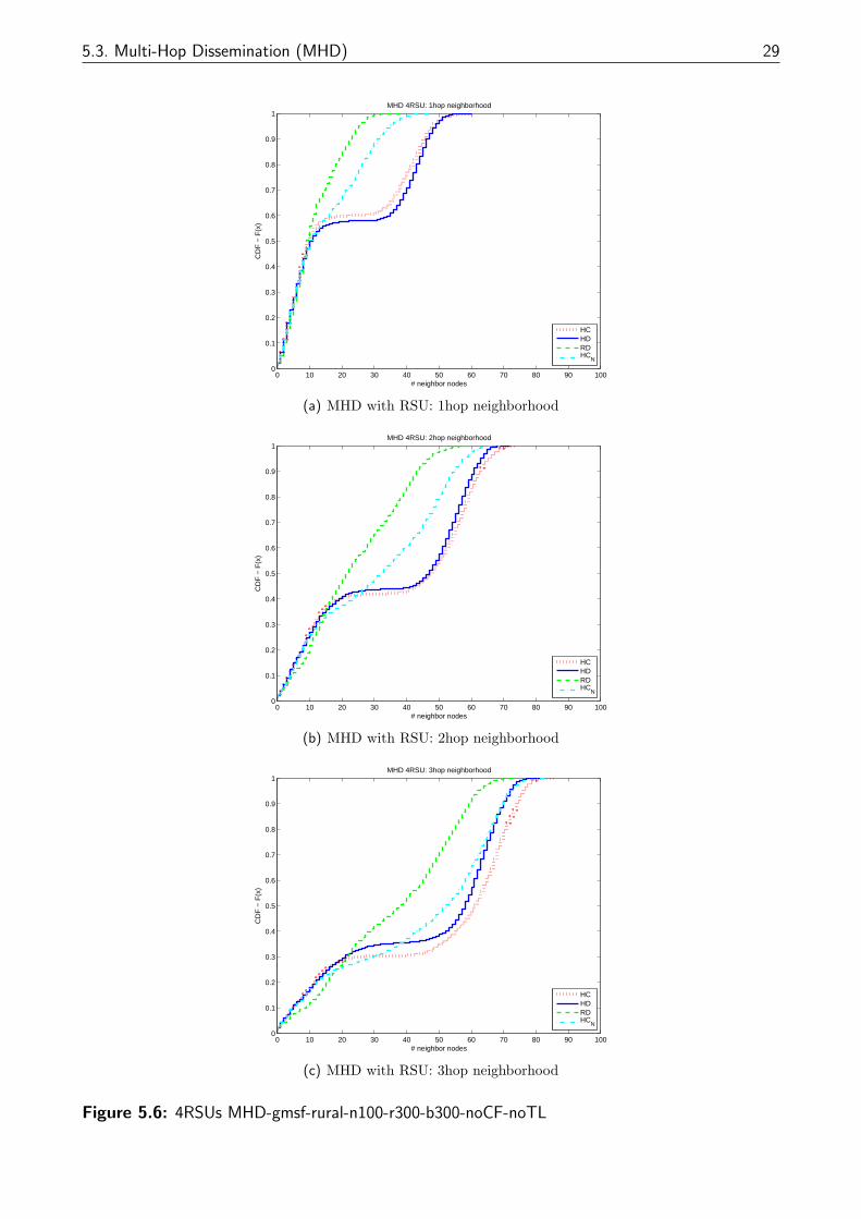
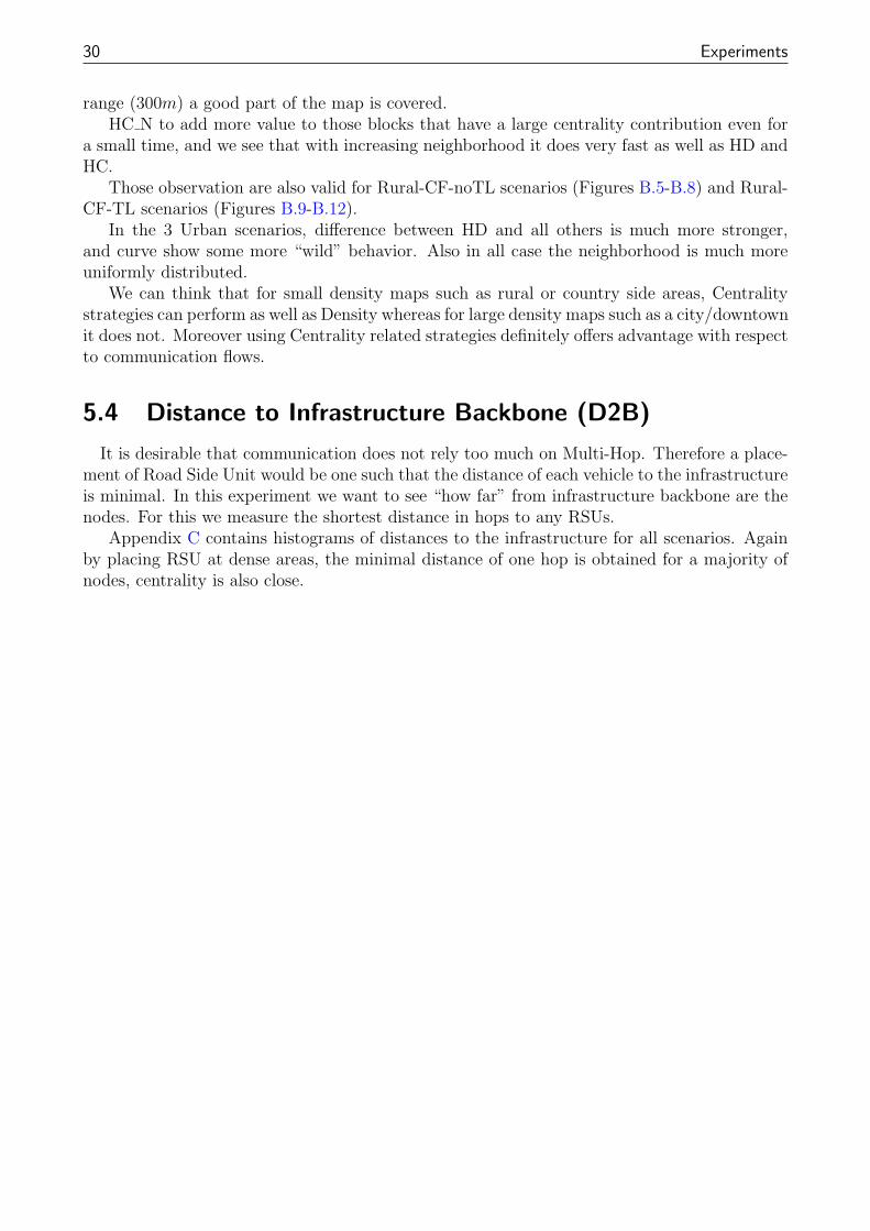
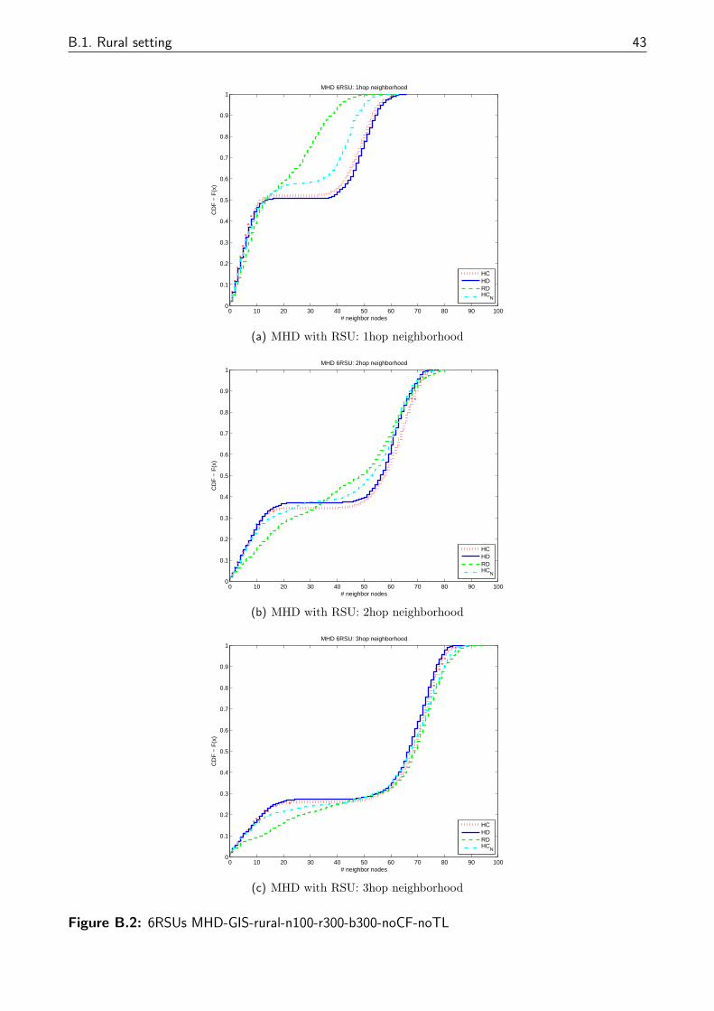
Then using information from the previous experiment where we found top dense/central blocksfor a map, does having road side unit nearby help in the dissemination? We used simple strate-gies described in 3.3 for the placement of RSUs. A common hypothesis is to place road sideunits at very dense places. We argue that central places might also be interesting since bydefinition those are the place that do “see” a lot of communication flow.
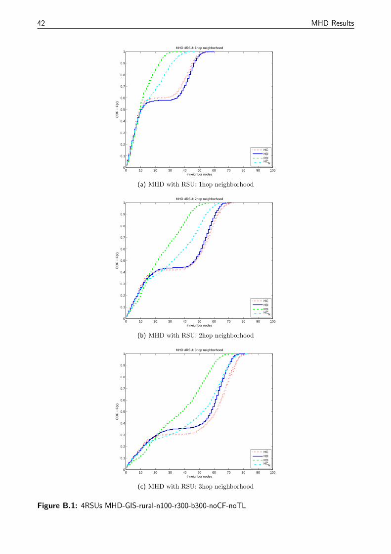
In appendix B we shows the distribution of the dissemination for all scenarios (rural, urban,city), all mobility models(noCF-noTL, CF-noTL, CF-TL) and for different RSUs number (4to 10). Cumulative Distribution Function (CDF) is on the Y-axis and the number of spreadneighbors on the X-axis.
Figure 5.6 shows Rural-noCF-noTL scenario with 4 RSUs. Other figures are in appendix B.With increasing neighborhood HC does as well as HD and even better in the 3hop-neighborhood.But the difference is very small if not negligible, for example, 90% of the nodes in HD have aneighborhood of 70 nodes or less whereas 90% of the nodes in HC strategy have a neighborhoodof 75 nodes or less. With the addition of more RSUs, the difference is even reduced, and allstrategies seems to have a similar distribution. This is due, too the fact that the set of denseblocks and central ones (in both HC and HC N) become similar as we increase the number ofRSU we want to place, and also that with more and more RSUs of quite large transmission
5.3. Multi-Hop Dissemination (MHD) 29
0 10 20 30 40 50 60 70 80 90 1000
0.1
0.2
0.3
0.4
0.5
0.6
0.7
0.8
0.9
1
# neighbor nodes
CD
F −
F(x
)
MHD 4RSU: 1hop neighborhood
HCHDRDHC
N
(a) MHD with RSU: 1hop neighborhood
0 10 20 30 40 50 60 70 80 90 1000
0.1
0.2
0.3
0.4
0.5
0.6
0.7
0.8
0.9
1
# neighbor nodes
CD
F −
F(x
)
MHD 4RSU: 2hop neighborhood
HCHDRDHC
N
(b) MHD with RSU: 2hop neighborhood
0 10 20 30 40 50 60 70 80 90 1000
0.1
0.2
0.3
0.4
0.5
0.6
0.7
0.8
0.9
1
# neighbor nodes
CD
F −
F(x
)
MHD 4RSU: 3hop neighborhood
HCHDRDHC
N
(c) MHD with RSU: 3hop neighborhood
Figure 5.6: 4RSUs MHD-gmsf-rural-n100-r300-b300-noCF-noTL
30 Experiments
range (300m) a good part of the map is covered.HC N to add more value to those blocks that have a large centrality contribution even for
a small time, and we see that with increasing neighborhood it does very fast as well as HD andHC.
Those observation are also valid for Rural-CF-noTL scenarios (Figures B.5-B.8) and Rural-CF-TL scenarios (Figures B.9-B.12).
In the 3 Urban scenarios, difference between HD and all others is much more stronger,and curve show some more “wild” behavior. Also in all case the neighborhood is much moreuniformly distributed.
We can think that for small density maps such as rural or country side areas, Centralitystrategies can perform as well as Density whereas for large density maps such as a city/downtownit does not. Moreover using Centrality related strategies definitely offers advantage with respectto communication flows.
5.4 Distance to Infrastructure Backbone (D2B)
It is desirable that communication does not rely too much on Multi-Hop. Therefore a place-ment of Road Side Unit would be one such that the distance of each vehicle to the infrastructureis minimal. In this experiment we want to see “how far” from infrastructure backbone are thenodes. For this we measure the shortest distance in hops to any RSUs.
Appendix C contains histograms of distances to the infrastructure for all scenarios. Againby placing RSU at dense areas, the minimal distance of one hop is obtained for a majority ofnodes, centrality is also close.
Chapter 6Conclusions and Future Work
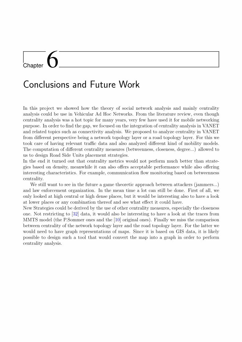
In this project we showed how the theory of social network analysis and mainly centralityanalysis could be use in Vehicular Ad Hoc Networks. From the literature review, even thoughcentrality analysis was a hot topic for many years, very few have used it for mobile networkingpurpose. In order to find the gap, we focused on the integration of centrality analysis in VANETand related topics such as connectivity analysis. We proposed to analyze centrality in VANETfrom different perspective being a network topology layer or a road topology layer. For this wetook care of having relevant traffic data and also analyzed different kind of mobility models.The computation of different centrality measures (betweenness, closeness, degree...) allowed tous to design Road Side Units placement strategies.In the end it turned out that centrality metrics would not perform much better than strate-gies based on density, meanwhile it can also offers acceptable performance while also offeringinteresting characteristics. For example, communication flow monitoring based on betweennesscentrality.
We still want to see in the future a game theoretic approach between attackers (jammers...)and law enforcement organization. In the mean time a lot can still be done. First of all, weonly looked at high central or high dense places, but it would be interesting also to have a lookat lower places or any combination thereof and see what effect it could have.New Strategies could be derived by the use of other centrality measures, especially the closenessone. Not restricting to [32] data, it would also be interesting to have a look at the traces fromMMTS model (the P.Sommer ones and the [10] original ones). Finally we miss the comparisonbetween centrality of the network topology layer and the road topology layer. For the latter wewould need to have graph representations of maps. Since it is based on GIS data, it is likelypossible to design such a tool that would convert the map into a graph in order to performcentrality analysis.

32 Conclusions and Future Work
Appendix ADCL Results
A.1 Rural setting
0 300 600 900 1200 1500 1800 2100 2400 2700 30000
300
600
900
1200
1500
1800
2100
2400
2700
3000Snapshot traffic process (t=500)
X−axis
Y−
axis
(a) Snapshot at t=500s
0300
600900
12001500
18002100
24002700
30003300
0300
600900
12001500
18002100
24002700
30003300
0
2
4
6
8
10
12
X−axis
Grid Density (#cars)
Y−axis
Ave
rage
nod
e de
nsity
(n
odes
/900
00m
2 )
(b) Grid Density
0300
600900
12001500
18002100
24002700
30003300
0300
600900
12001500
18002100
24002700
30003300
0
0.5
1
1.5
2
2.5
3
3.5
x 106
X−axis
Grid Betweenness Centrality (CB)
Y−axis
Sum
of C
B A
ctor
Indi
ces
(c) Grid Betweenness
0300
600900
12001500
18002100
24002700
30003300
0300
600900
12001500
18002100
24002700
30003300
0
100
200
300
400
500
600
X−axis
Grid Betweenness Centrlity Normalized
Y−axis
Ave
rage
CB A
ctor
Inde
x p
er n
ode
in a
rea
(d) Grid Betweenness Normalized
Figure A.1: GIS-rural-n100-r300-b300-noCF-noTL
34 DCL Results
0 300 600 900 1200 1500 1800 2100 2400 2700 30000
300
600
900
1200
1500
1800
2100
2400
2700
3000Snapshot traffic process (t=500)
X−axis
Y−
axis
(a) Snapshot at t=500s
0300
600900
12001500
18002100
24002700
30003300
0300
600900
12001500
18002100
24002700
30003300
0
5
10
15
20
X−axis
Grid Density (#cars)
Y−axis
Ave
rage
nod
e de
nsity
(n
odes
/900
00m
2 )
(b) Grid Density
0300
600900
12001500
18002100
24002700
30003300
0300
600900
12001500
18002100
24002700
30003300
0
0.5
1
1.5
2
2.5
3
3.5
x 106
X−axis
Grid Betweenness Centrality (CB)
Y−axis
Sum
of C
B A
ctor
Indi
ces
(c) Grid Betweenness
0300
600900
12001500
18002100
24002700
30003300
0300
600900
12001500
18002100
24002700
30003300
0
100
200
300
400
500
600
X−axis
Grid Betweenness Centrlity Normalized
Y−axis
Ave
rage
CB A
ctor
Inde
x p
er n
ode
in a
rea
(d) Grid Betweenness Normalized
Figure A.2: GIS-rural-n100-r300-b300-CF-noTL
A.1. Rural setting 35
0 300 600 900 1200 1500 1800 2100 2400 2700 30000
300
600
900
1200
1500
1800
2100
2400
2700
3000Snapshot traffic process (t=500)
X−axis
Y−
axis
(a) Snapshot at t=500s
0300
600900
12001500
18002100
24002700
30003300
0300
600900
12001500
18002100
24002700
30003300
0
5
10
15
20
25
30
X−axis
Grid Density (#cars)
Y−axis
Ave
rage
nod
e de
nsity
(n
odes
/900
00m
2 )
(b) Grid Density
0300
600900
12001500
18002100
24002700
30003300
0300
600900
12001500
18002100
24002700
30003300
0
0.5
1
1.5
2
2.5
x 106
X−axis
Grid Betweenness Centrality (CB)
Y−axis
Sum
of C
B A
ctor
Indi
ces
(c) Grid Betweenness
0300
600900
12001500
18002100
24002700
30003300
0300
600900
12001500
18002100
24002700
30003300
0
100
200
300
400
X−axis
Grid Betweenness Centrlity Normalized
Y−axis
Ave
rage
CB A
ctor
Inde
x p
er n
ode
in a
rea
(d) Grid Betweenness Normalized
Figure A.3: GIS-rural-n100-r300-b300-CF-TL

36 DCL Results
A.2. Urban setting 37
A.2 Urban setting
0 300 600 900 1200 1500 1800 2100 2400 2700 30000
300
600
900
1200
1500
1800
2100
2400
2700
3000Snapshot traffic process (t=500)
X−axis
Y−
axis
(a) Snapshot at t=500s
0300
600900
12001500
18002100
24002700
30003300
0300
600900
12001500
18002100
24002700
30003300
0
5
10
15
20
25
X−axis
Grid Density (#cars)
Y−axis
Ave
rage
nod
e de
nsity
(n
odes
/900
00m
2 )
(b) Grid Density
0300
600900
12001500
18002100
24002700
30003300
0300
600900
12001500
18002100
24002700
30003300
0
1
2
3
4
5
6
x 107
X−axis
Grid Betweenness Centrality (CB)
Y−axis
Sum
of C
B A
ctor
Indi
ces
(c) Grid Betweenness
0300
600900
12001500
18002100
24002700
30003300
0300
600900
12001500
18002100
24002700
30003300
0
1000
2000
3000
4000
X−axis
Grid Betweenness Centrlity Normalized
Y−axis
Ave
rage
CB A
ctor
Inde
x p
er n
ode
in a
rea
(d) Grid Betweenness Normalized
Figure A.4: GIS-urban-n420-r300-b300-noCF-noTL
38 DCL Results
0 300 600 900 1200 1500 1800 2100 2400 2700 30000
300
600
900
1200
1500
1800
2100
2400
2700
3000Snapshot traffic process (t=500)
X−axis
Y−
axis
(a) Snapshot at t=500s
0300
600900
12001500
18002100
24002700
30003300
0300
600900
12001500
18002100
24002700
30003300
0
5
10
15
20
25
30
35
X−axis
Grid Density (#cars)
Y−axis
Ave
rage
nod
e de
nsity
(n
odes
/900
00m
2 )
(b) Grid Density
0300
600900
12001500
18002100
24002700
30003300
0300
600900
12001500
18002100
24002700
30003300
0
1
2
3
4
5
6
7
x 107
X−axis
Grid Betweenness Centrality (CB)
Y−axis
Sum
of C
B A
ctor
Indi
ces
(c) Grid Betweenness
0300
600900
12001500
18002100
24002700
30003300
0300
600900
12001500
18002100
24002700
30003300
0
1000
2000
3000
4000
X−axis
Grid Betweenness Centrlity Normalized
Y−axis
Ave
rage
CB A
ctor
Inde
x p
er n
ode
in a
rea
(d) Grid Betweenness Normalized
Figure A.5: GIS-urban-n420-r300-b300-CF-noTL

A.3. City setting 39
A.3 City setting

40 DCL Results
Appendix BMHD Results
B.1 Rural setting
B.1.1 noCF-noTL
42 MHD Results
0 10 20 30 40 50 60 70 80 90 1000
0.1
0.2
0.3
0.4
0.5
0.6
0.7
0.8
0.9
1
# neighbor nodes
CD
F −
F(x
)
MHD 4RSU: 1hop neighborhood
HCHDRDHC
N
(a) MHD with RSU: 1hop neighborhood
0 10 20 30 40 50 60 70 80 90 1000
0.1
0.2
0.3
0.4
0.5
0.6
0.7
0.8
0.9
1
# neighbor nodes
CD
F −
F(x
)
MHD 4RSU: 2hop neighborhood
HCHDRDHC
N
(b) MHD with RSU: 2hop neighborhood
0 10 20 30 40 50 60 70 80 90 1000
0.1
0.2
0.3
0.4
0.5
0.6
0.7
0.8
0.9
1
# neighbor nodes
CD
F −
F(x
)
MHD 4RSU: 3hop neighborhood
HCHDRDHC
N
(c) MHD with RSU: 3hop neighborhood
Figure B.1: 4RSUs MHD-GIS-rural-n100-r300-b300-noCF-noTL
B.1. Rural setting 43
0 10 20 30 40 50 60 70 80 90 1000
0.1
0.2
0.3
0.4
0.5
0.6
0.7
0.8
0.9
1
# neighbor nodes
CD
F −
F(x
)
MHD 6RSU: 1hop neighborhood
HCHDRDHC
N
(a) MHD with RSU: 1hop neighborhood
0 10 20 30 40 50 60 70 80 90 1000
0.1
0.2
0.3
0.4
0.5
0.6
0.7
0.8
0.9
1
# neighbor nodes
CD
F −
F(x
)
MHD 6RSU: 2hop neighborhood
HCHDRDHC
N
(b) MHD with RSU: 2hop neighborhood
0 10 20 30 40 50 60 70 80 90 1000
0.1
0.2
0.3
0.4
0.5
0.6
0.7
0.8
0.9
1
# neighbor nodes
CD
F −
F(x
)
MHD 6RSU: 3hop neighborhood
HCHDRDHC
N
(c) MHD with RSU: 3hop neighborhood
Figure B.2: 6RSUs MHD-GIS-rural-n100-r300-b300-noCF-noTL
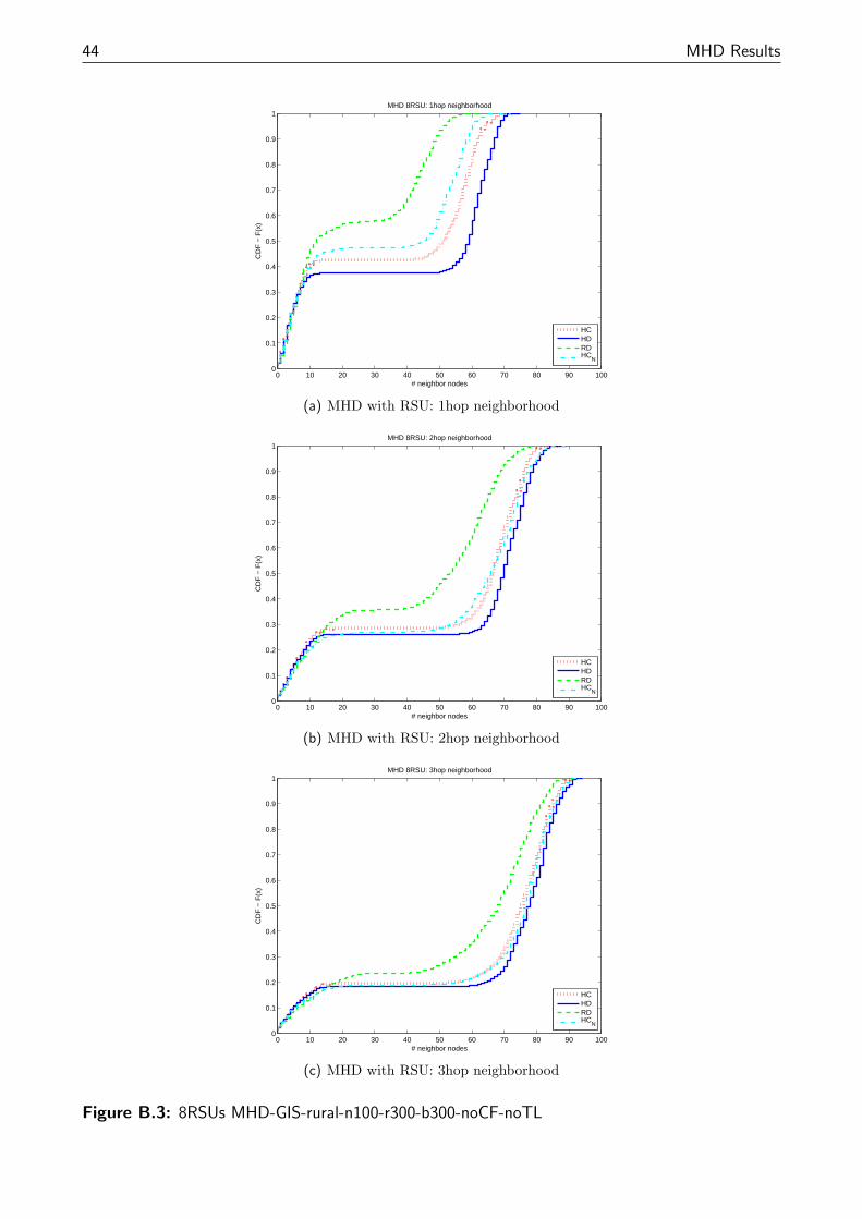
44 MHD Results
0 10 20 30 40 50 60 70 80 90 1000
0.1
0.2
0.3
0.4
0.5
0.6
0.7
0.8
0.9
1
# neighbor nodes
CD
F −
F(x
)
MHD 8RSU: 1hop neighborhood
HCHDRDHC
N
(a) MHD with RSU: 1hop neighborhood
0 10 20 30 40 50 60 70 80 90 1000
0.1
0.2
0.3
0.4
0.5
0.6
0.7
0.8
0.9
1
# neighbor nodes
CD
F −
F(x
)
MHD 8RSU: 2hop neighborhood
HCHDRDHC
N
(b) MHD with RSU: 2hop neighborhood
0 10 20 30 40 50 60 70 80 90 1000
0.1
0.2
0.3
0.4
0.5
0.6
0.7
0.8
0.9
1
# neighbor nodes
CD
F −
F(x
)
MHD 8RSU: 3hop neighborhood
HCHDRDHC
N
(c) MHD with RSU: 3hop neighborhood
Figure B.3: 8RSUs MHD-GIS-rural-n100-r300-b300-noCF-noTL

B.1. Rural setting 45
0 10 20 30 40 50 60 70 80 90 1000
0.1
0.2
0.3
0.4
0.5
0.6
0.7
0.8
0.9
1
# neighbor nodes
CD
F −
F(x
)
MHD 10RSU: 1hop neighborhood
HCHDRDHC
N
(a) MHD with RSU: 1hop neighborhood
0 10 20 30 40 50 60 70 80 90 1000
0.1
0.2
0.3
0.4
0.5
0.6
0.7
0.8
0.9
1
# neighbor nodes
CD
F −
F(x
)
MHD 10RSU: 2hop neighborhood
HCHDRDHC
N
(b) MHD with RSU: 2hop neighborhood
0 10 20 30 40 50 60 70 80 90 1000
0.1
0.2
0.3
0.4
0.5
0.6
0.7
0.8
0.9
1
# neighbor nodes
CD
F −
F(x
)
MHD 10RSU: 3hop neighborhood
HCHDRDHC
N
(c) MHD with RSU: 3hop neighborhood
Figure B.4: 10RSUs MHD-GIS-rural-n100-r300-b300-noCF-noTL

46 MHD Results
B.1.2 CF-noTL

B.1. Rural setting 47
0 10 20 30 40 50 60 70 80 90 1000
0.1
0.2
0.3
0.4
0.5
0.6
0.7
0.8
0.9
1
# neighbor nodes
CD
F −
F(x
)
MHD 4RSU: 1hop neighborhood
HCHDRDHC
N
(a) MHD with RSU: 1hop neighborhood
0 10 20 30 40 50 60 70 80 90 1000
0.1
0.2
0.3
0.4
0.5
0.6
0.7
0.8
0.9
1
# neighbor nodes
CD
F −
F(x
)
MHD 4RSU: 2hop neighborhood
HCHDRDHC
N
(b) MHD with RSU: 2hop neighborhood
0 10 20 30 40 50 60 70 80 90 1000
0.1
0.2
0.3
0.4
0.5
0.6
0.7
0.8
0.9
1
# neighbor nodes
CD
F −
F(x
)
MHD 4RSU: 3hop neighborhood
HCHDRDHC
N
(c) MHD with RSU: 3hop neighborhood
Figure B.5: 4RSUs MHD-GIS-rural-n100-r300-b300-CF-noTL
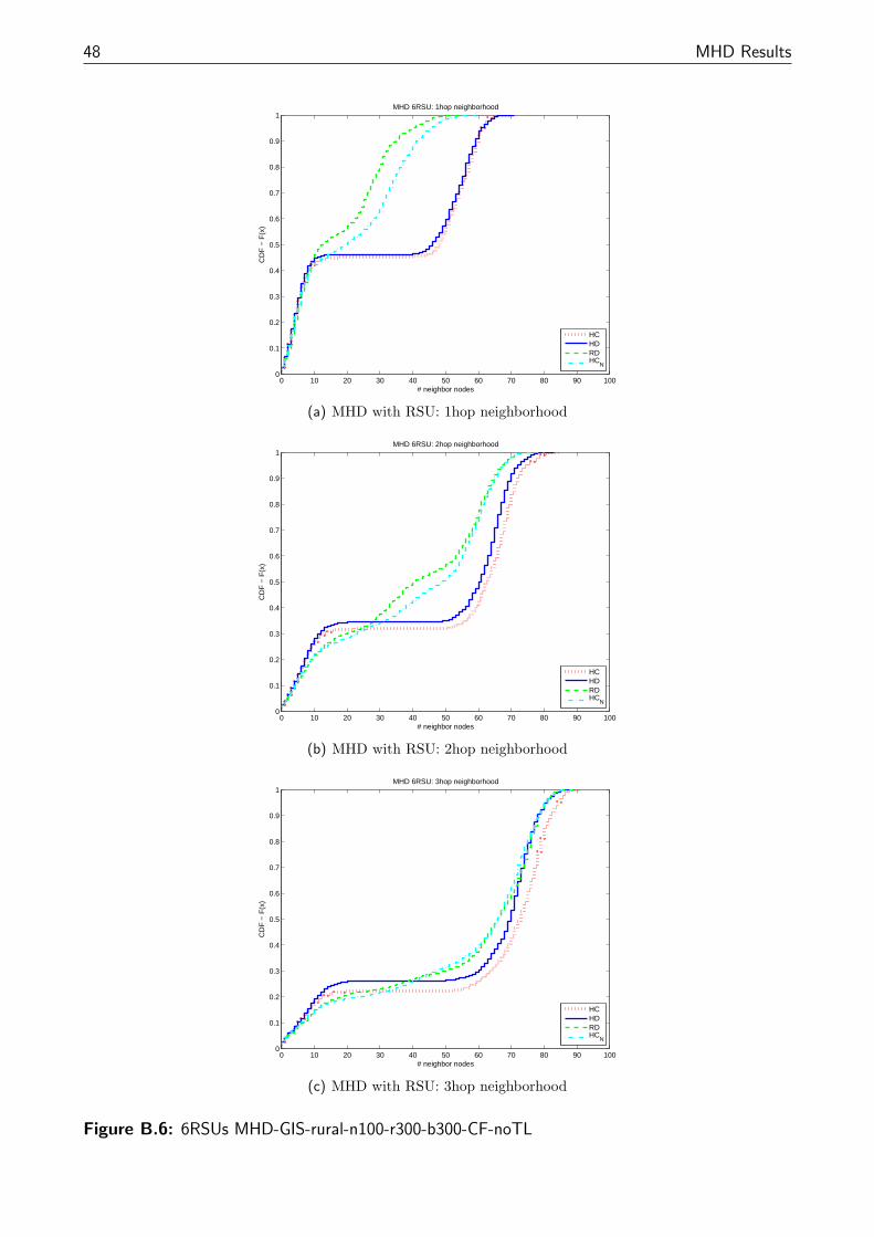
48 MHD Results
0 10 20 30 40 50 60 70 80 90 1000
0.1
0.2
0.3
0.4
0.5
0.6
0.7
0.8
0.9
1
# neighbor nodes
CD
F −
F(x
)
MHD 6RSU: 1hop neighborhood
HCHDRDHC
N
(a) MHD with RSU: 1hop neighborhood
0 10 20 30 40 50 60 70 80 90 1000
0.1
0.2
0.3
0.4
0.5
0.6
0.7
0.8
0.9
1
# neighbor nodes
CD
F −
F(x
)
MHD 6RSU: 2hop neighborhood
HCHDRDHC
N
(b) MHD with RSU: 2hop neighborhood
0 10 20 30 40 50 60 70 80 90 1000
0.1
0.2
0.3
0.4
0.5
0.6
0.7
0.8
0.9
1
# neighbor nodes
CD
F −
F(x
)
MHD 6RSU: 3hop neighborhood
HCHDRDHC
N
(c) MHD with RSU: 3hop neighborhood
Figure B.6: 6RSUs MHD-GIS-rural-n100-r300-b300-CF-noTL

B.1. Rural setting 49
0 10 20 30 40 50 60 70 80 90 1000
0.1
0.2
0.3
0.4
0.5
0.6
0.7
0.8
0.9
1
# neighbor nodes
CD
F −
F(x
)
MHD 8RSU: 1hop neighborhood
HCHDRDHC
N
(a) MHD with RSU: 1hop neighborhood
0 10 20 30 40 50 60 70 80 90 1000
0.1
0.2
0.3
0.4
0.5
0.6
0.7
0.8
0.9
1
# neighbor nodes
CD
F −
F(x
)
MHD 8RSU: 2hop neighborhood
HCHDRDHC
N
(b) MHD with RSU: 2hop neighborhood
0 10 20 30 40 50 60 70 80 90 1000
0.1
0.2
0.3
0.4
0.5
0.6
0.7
0.8
0.9
1
# neighbor nodes
CD
F −
F(x
)
MHD 8RSU: 3hop neighborhood
HCHDRDHC
N
(c) MHD with RSU: 3hop neighborhood
Figure B.7: 8RSUs MHD-GIS-rural-n100-r300-b300-CF-noTL
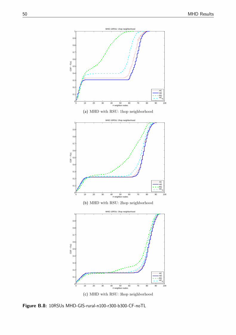
50 MHD Results
0 10 20 30 40 50 60 70 80 90 1000
0.1
0.2
0.3
0.4
0.5
0.6
0.7
0.8
0.9
1
# neighbor nodes
CD
F −
F(x
)
MHD 10RSU: 1hop neighborhood
HCHDRDHC
N
(a) MHD with RSU: 1hop neighborhood
0 10 20 30 40 50 60 70 80 90 1000
0.1
0.2
0.3
0.4
0.5
0.6
0.7
0.8
0.9
1
# neighbor nodes
CD
F −
F(x
)
MHD 10RSU: 2hop neighborhood
HCHDRDHC
N
(b) MHD with RSU: 2hop neighborhood
0 10 20 30 40 50 60 70 80 90 1000
0.1
0.2
0.3
0.4
0.5
0.6
0.7
0.8
0.9
1
# neighbor nodes
CD
F −
F(x
)
MHD 10RSU: 3hop neighborhood
HCHDRDHC
N
(c) MHD with RSU: 3hop neighborhood
Figure B.8: 10RSUs MHD-GIS-rural-n100-r300-b300-CF-noTL

B.1. Rural setting 51
B.1.3 CF-TL
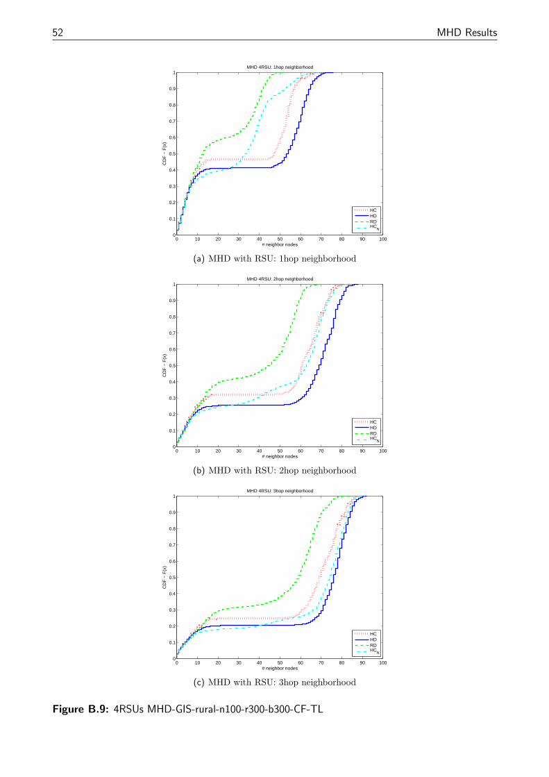
52 MHD Results
0 10 20 30 40 50 60 70 80 90 1000
0.1
0.2
0.3
0.4
0.5
0.6
0.7
0.8
0.9
1
# neighbor nodes
CD
F −
F(x
)
MHD 4RSU: 1hop neighborhood
HCHDRDHC
N
(a) MHD with RSU: 1hop neighborhood
0 10 20 30 40 50 60 70 80 90 1000
0.1
0.2
0.3
0.4
0.5
0.6
0.7
0.8
0.9
1
# neighbor nodes
CD
F −
F(x
)
MHD 4RSU: 2hop neighborhood
HCHDRDHC
N
(b) MHD with RSU: 2hop neighborhood
0 10 20 30 40 50 60 70 80 90 1000
0.1
0.2
0.3
0.4
0.5
0.6
0.7
0.8
0.9
1
# neighbor nodes
CD
F −
F(x
)
MHD 4RSU: 3hop neighborhood
HCHDRDHC
N
(c) MHD with RSU: 3hop neighborhood
Figure B.9: 4RSUs MHD-GIS-rural-n100-r300-b300-CF-TL

B.1. Rural setting 53
0 10 20 30 40 50 60 70 80 90 1000
0.1
0.2
0.3
0.4
0.5
0.6
0.7
0.8
0.9
1
# neighbor nodes
CD
F −
F(x
)
MHD 6RSU: 1hop neighborhood
HCHDRDHC
N
(a) MHD with RSU: 1hop neighborhood
0 10 20 30 40 50 60 70 80 90 1000
0.1
0.2
0.3
0.4
0.5
0.6
0.7
0.8
0.9
1
# neighbor nodes
CD
F −
F(x
)
MHD 6RSU: 2hop neighborhood
HCHDRDHC
N
(b) MHD with RSU: 2hop neighborhood
0 10 20 30 40 50 60 70 80 90 1000
0.1
0.2
0.3
0.4
0.5
0.6
0.7
0.8
0.9
1
# neighbor nodes
CD
F −
F(x
)
MHD 6RSU: 3hop neighborhood
HCHDRDHC
N
(c) MHD with RSU: 3hop neighborhood
Figure B.10: 6RSUs MHD-GIS-rural-n100-r300-b300-CF-TL
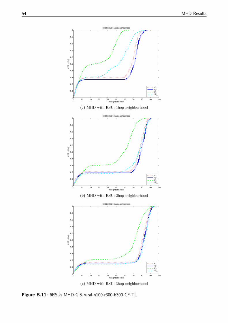
54 MHD Results
0 10 20 30 40 50 60 70 80 90 1000
0.1
0.2
0.3
0.4
0.5
0.6
0.7
0.8
0.9
1
# neighbor nodes
CD
F −
F(x
)
MHD 8RSU: 1hop neighborhood
HCHDRDHC
N
(a) MHD with RSU: 1hop neighborhood
0 10 20 30 40 50 60 70 80 90 1000
0.1
0.2
0.3
0.4
0.5
0.6
0.7
0.8
0.9
1
# neighbor nodes
CD
F −
F(x
)
MHD 8RSU: 2hop neighborhood
HCHDRDHC
N
(b) MHD with RSU: 2hop neighborhood
0 10 20 30 40 50 60 70 80 90 1000
0.1
0.2
0.3
0.4
0.5
0.6
0.7
0.8
0.9
1
# neighbor nodes
CD
F −
F(x
)
MHD 8RSU: 3hop neighborhood
HCHDRDHC
N
(c) MHD with RSU: 3hop neighborhood
Figure B.11: 6RSUs MHD-GIS-rural-n100-r300-b300-CF-TL
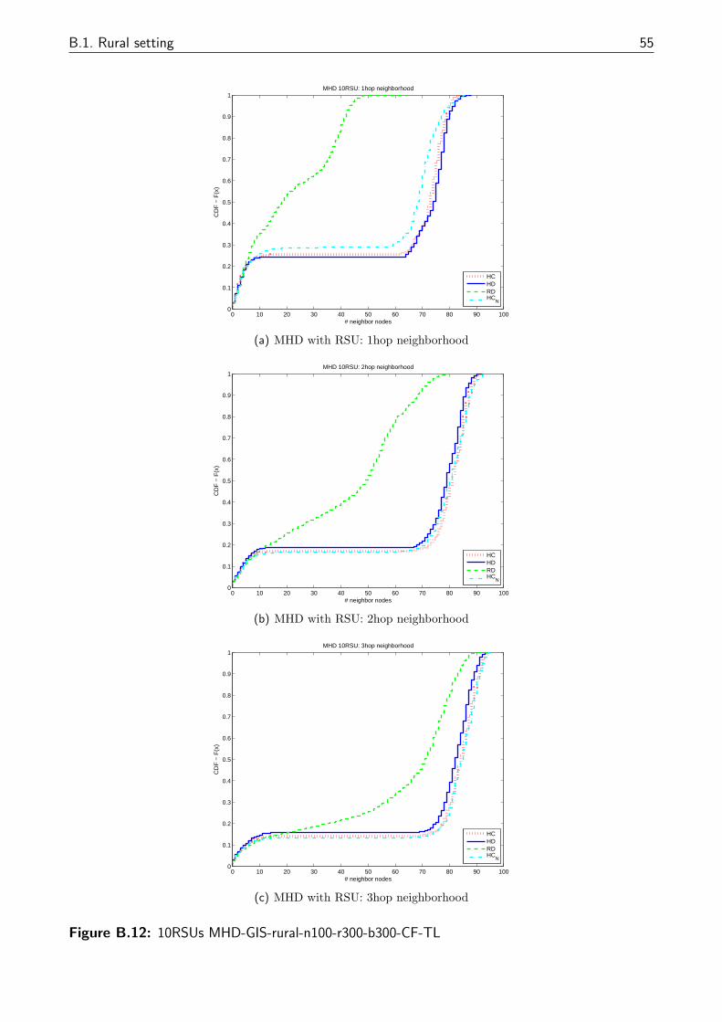
B.1. Rural setting 55
0 10 20 30 40 50 60 70 80 90 1000
0.1
0.2
0.3
0.4
0.5
0.6
0.7
0.8
0.9
1
# neighbor nodes
CD
F −
F(x
)
MHD 10RSU: 1hop neighborhood
HCHDRDHC
N
(a) MHD with RSU: 1hop neighborhood
0 10 20 30 40 50 60 70 80 90 1000
0.1
0.2
0.3
0.4
0.5
0.6
0.7
0.8
0.9
1
# neighbor nodes
CD
F −
F(x
)
MHD 10RSU: 2hop neighborhood
HCHDRDHC
N
(b) MHD with RSU: 2hop neighborhood
0 10 20 30 40 50 60 70 80 90 1000
0.1
0.2
0.3
0.4
0.5
0.6
0.7
0.8
0.9
1
# neighbor nodes
CD
F −
F(x
)
MHD 10RSU: 3hop neighborhood
HCHDRDHC
N
(c) MHD with RSU: 3hop neighborhood
Figure B.12: 10RSUs MHD-GIS-rural-n100-r300-b300-CF-TL

56 MHD Results
B.2 Urban setting
B.2.1 noCF-noTL

B.2. Urban setting 57
0 50 100 150 200 250 300 350 4000
0.1
0.2
0.3
0.4
0.5
0.6
0.7
0.8
0.9
1
# neighbor nodes
CD
F −
F(x
)
MHD 4RSU: 1hop neighborhood
HCHDRDHC
N
(a) MHD with RSU: 1hop neighborhood
0 50 100 150 200 250 300 350 4000
0.1
0.2
0.3
0.4
0.5
0.6
0.7
0.8
0.9
1
# neighbor nodes
CD
F −
F(x
)
MHD 4RSU: 2hop neighborhood
HCHDRDHC
N
(b) MHD with RSU: 2hop neighborhood
0 50 100 150 200 250 300 350 4000
0.1
0.2
0.3
0.4
0.5
0.6
0.7
0.8
0.9
1
# neighbor nodes
CD
F −
F(x
)
MHD 4RSU: 3hop neighborhood
HCHDRDHC
N
(c) MHD with RSU: 3hop neighborhood
Figure B.13: 4RSUs MHD-GIS-urban-n420-r300-b300-noCF-noTL
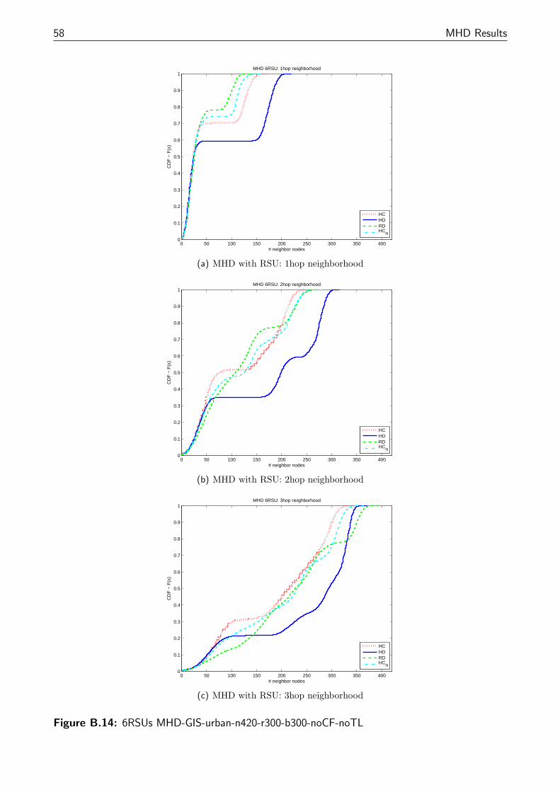
58 MHD Results
0 50 100 150 200 250 300 350 4000
0.1
0.2
0.3
0.4
0.5
0.6
0.7
0.8
0.9
1
# neighbor nodes
CD
F −
F(x
)
MHD 6RSU: 1hop neighborhood
HCHDRDHC
N
(a) MHD with RSU: 1hop neighborhood
0 50 100 150 200 250 300 350 4000
0.1
0.2
0.3
0.4
0.5
0.6
0.7
0.8
0.9
1
# neighbor nodes
CD
F −
F(x
)
MHD 6RSU: 2hop neighborhood
HCHDRDHC
N
(b) MHD with RSU: 2hop neighborhood
0 50 100 150 200 250 300 350 4000
0.1
0.2
0.3
0.4
0.5
0.6
0.7
0.8
0.9
1
# neighbor nodes
CD
F −
F(x
)
MHD 6RSU: 3hop neighborhood
HCHDRDHC
N
(c) MHD with RSU: 3hop neighborhood
Figure B.14: 6RSUs MHD-GIS-urban-n420-r300-b300-noCF-noTL
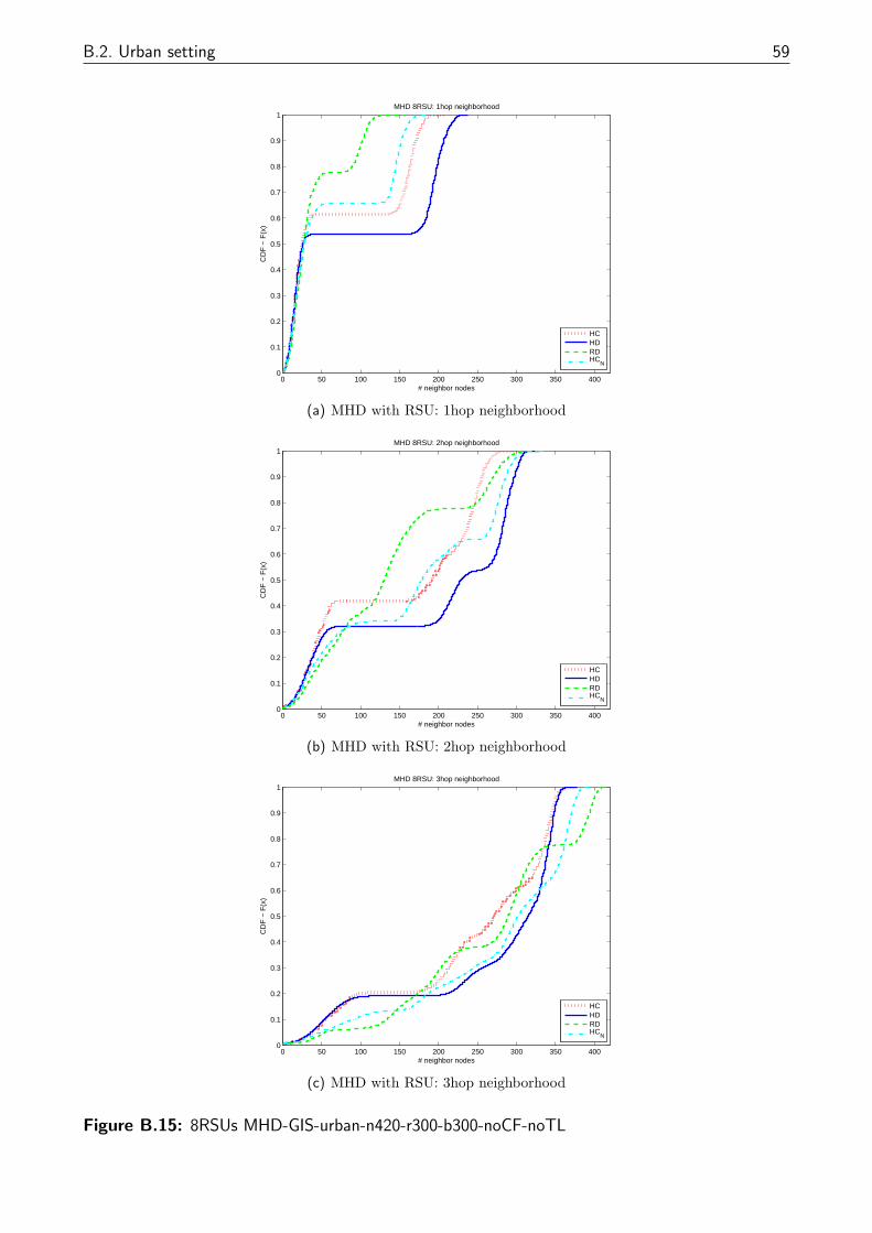
B.2. Urban setting 59
0 50 100 150 200 250 300 350 4000
0.1
0.2
0.3
0.4
0.5
0.6
0.7
0.8
0.9
1
# neighbor nodes
CD
F −
F(x
)
MHD 8RSU: 1hop neighborhood
HCHDRDHC
N
(a) MHD with RSU: 1hop neighborhood
0 50 100 150 200 250 300 350 4000
0.1
0.2
0.3
0.4
0.5
0.6
0.7
0.8
0.9
1
# neighbor nodes
CD
F −
F(x
)
MHD 8RSU: 2hop neighborhood
HCHDRDHC
N
(b) MHD with RSU: 2hop neighborhood
0 50 100 150 200 250 300 350 4000
0.1
0.2
0.3
0.4
0.5
0.6
0.7
0.8
0.9
1
# neighbor nodes
CD
F −
F(x
)
MHD 8RSU: 3hop neighborhood
HCHDRDHC
N
(c) MHD with RSU: 3hop neighborhood
Figure B.15: 8RSUs MHD-GIS-urban-n420-r300-b300-noCF-noTL

60 MHD Results
0 50 100 150 200 250 300 350 4000
0.1
0.2
0.3
0.4
0.5
0.6
0.7
0.8
0.9
1
# neighbor nodes
CD
F −
F(x
)
MHD 10RSU: 1hop neighborhood
HCHDRDHC
N
(a) MHD with RSU: 1hop neighborhood
0 50 100 150 200 250 300 350 4000
0.1
0.2
0.3
0.4
0.5
0.6
0.7
0.8
0.9
1
# neighbor nodes
CD
F −
F(x
)
MHD 10RSU: 2hop neighborhood
HCHDRDHC
N
(b) MHD with RSU: 2hop neighborhood
0 50 100 150 200 250 300 350 4000
0.1
0.2
0.3
0.4
0.5
0.6
0.7
0.8
0.9
1
# neighbor nodes
CD
F −
F(x
)
MHD 10RSU: 3hop neighborhood
HCHDRDHC
N
(c) MHD with RSU: 3hop neighborhood
Figure B.16: 10RSUs MHD-gmsf-urban-n420-r300-b300-noCF-noTL

B.2. Urban setting 61
B.2.2 CF-noTL
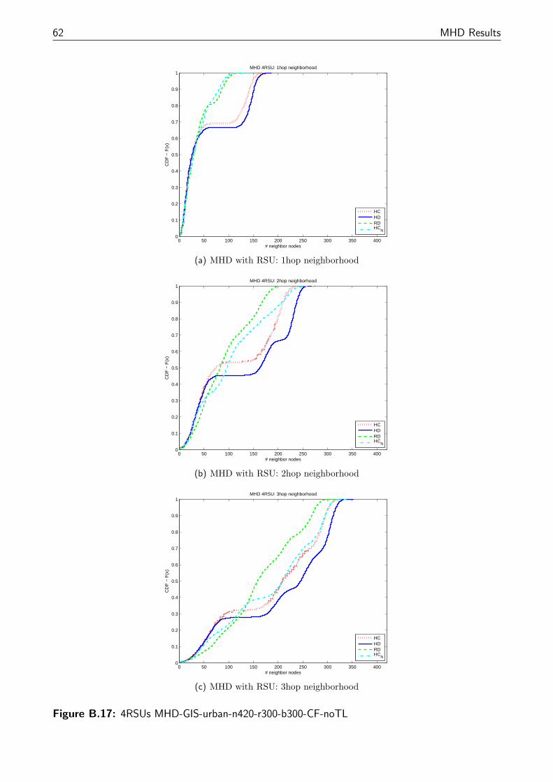
62 MHD Results
0 50 100 150 200 250 300 350 4000
0.1
0.2
0.3
0.4
0.5
0.6
0.7
0.8
0.9
1
# neighbor nodes
CD
F −
F(x
)
MHD 4RSU: 1hop neighborhood
HCHDRDHC
N
(a) MHD with RSU: 1hop neighborhood
0 50 100 150 200 250 300 350 4000
0.1
0.2
0.3
0.4
0.5
0.6
0.7
0.8
0.9
1
# neighbor nodes
CD
F −
F(x
)
MHD 4RSU: 2hop neighborhood
HCHDRDHC
N
(b) MHD with RSU: 2hop neighborhood
0 50 100 150 200 250 300 350 4000
0.1
0.2
0.3
0.4
0.5
0.6
0.7
0.8
0.9
1
# neighbor nodes
CD
F −
F(x
)
MHD 4RSU: 3hop neighborhood
HCHDRDHC
N
(c) MHD with RSU: 3hop neighborhood
Figure B.17: 4RSUs MHD-GIS-urban-n420-r300-b300-CF-noTL
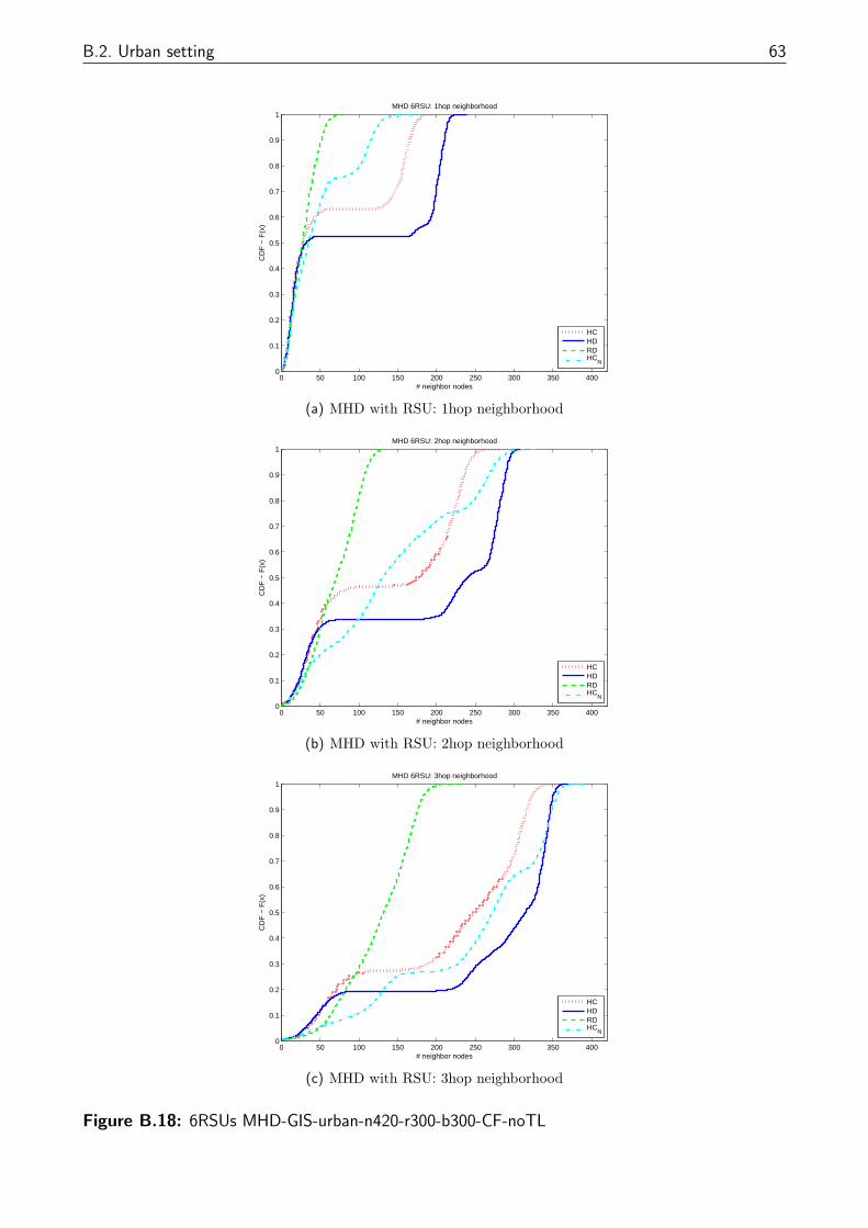
B.2. Urban setting 63
0 50 100 150 200 250 300 350 4000
0.1
0.2
0.3
0.4
0.5
0.6
0.7
0.8
0.9
1
# neighbor nodes
CD
F −
F(x
)
MHD 6RSU: 1hop neighborhood
HCHDRDHC
N
(a) MHD with RSU: 1hop neighborhood
0 50 100 150 200 250 300 350 4000
0.1
0.2
0.3
0.4
0.5
0.6
0.7
0.8
0.9
1
# neighbor nodes
CD
F −
F(x
)
MHD 6RSU: 2hop neighborhood
HCHDRDHC
N
(b) MHD with RSU: 2hop neighborhood
0 50 100 150 200 250 300 350 4000
0.1
0.2
0.3
0.4
0.5
0.6
0.7
0.8
0.9
1
# neighbor nodes
CD
F −
F(x
)
MHD 6RSU: 3hop neighborhood
HCHDRDHC
N
(c) MHD with RSU: 3hop neighborhood
Figure B.18: 6RSUs MHD-GIS-urban-n420-r300-b300-CF-noTL
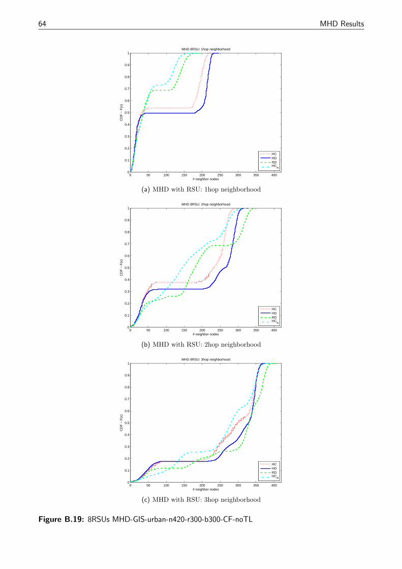
64 MHD Results
0 50 100 150 200 250 300 350 4000
0.1
0.2
0.3
0.4
0.5
0.6
0.7
0.8
0.9
1
# neighbor nodes
CD
F −
F(x
)
MHD 8RSU: 1hop neighborhood
HCHDRDHC
N
(a) MHD with RSU: 1hop neighborhood
0 50 100 150 200 250 300 350 4000
0.1
0.2
0.3
0.4
0.5
0.6
0.7
0.8
0.9
1
# neighbor nodes
CD
F −
F(x
)
MHD 8RSU: 2hop neighborhood
HCHDRDHC
N
(b) MHD with RSU: 2hop neighborhood
0 50 100 150 200 250 300 350 4000
0.1
0.2
0.3
0.4
0.5
0.6
0.7
0.8
0.9
1
# neighbor nodes
CD
F −
F(x
)
MHD 8RSU: 3hop neighborhood
HCHDRDHC
N
(c) MHD with RSU: 3hop neighborhood
Figure B.19: 8RSUs MHD-GIS-urban-n420-r300-b300-CF-noTL
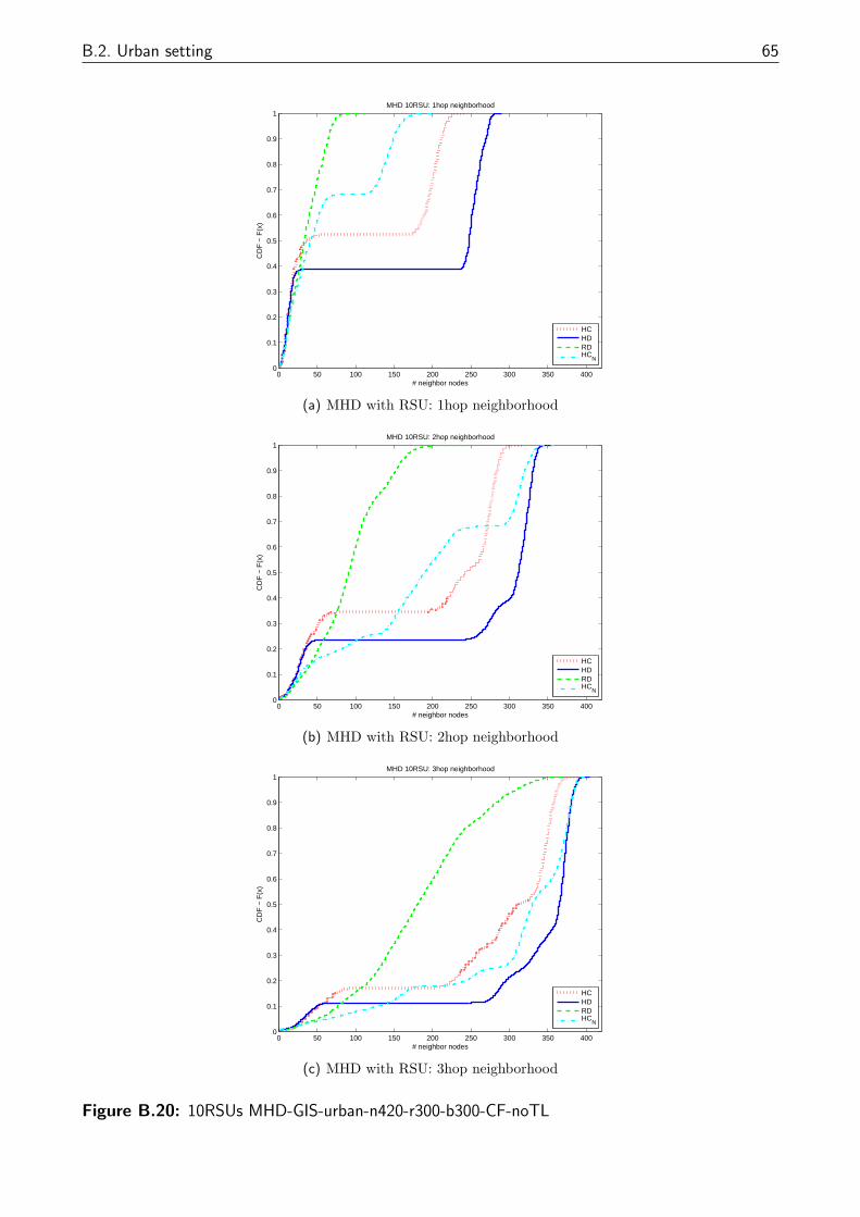
B.2. Urban setting 65
0 50 100 150 200 250 300 350 4000
0.1
0.2
0.3
0.4
0.5
0.6
0.7
0.8
0.9
1
# neighbor nodes
CD
F −
F(x
)
MHD 10RSU: 1hop neighborhood
HCHDRDHC
N
(a) MHD with RSU: 1hop neighborhood
0 50 100 150 200 250 300 350 4000
0.1
0.2
0.3
0.4
0.5
0.6
0.7
0.8
0.9
1
# neighbor nodes
CD
F −
F(x
)
MHD 10RSU: 2hop neighborhood
HCHDRDHC
N
(b) MHD with RSU: 2hop neighborhood
0 50 100 150 200 250 300 350 4000
0.1
0.2
0.3
0.4
0.5
0.6
0.7
0.8
0.9
1
# neighbor nodes
CD
F −
F(x
)
MHD 10RSU: 3hop neighborhood
HCHDRDHC
N
(c) MHD with RSU: 3hop neighborhood
Figure B.20: 10RSUs MHD-GIS-urban-n420-r300-b300-CF-noTL

66 MHD Results
B.2.3 CF-TL
B.3. City setting 67
B.3 City setting
B.3.1 noCF-noTL

68 MHD Results
B.3.2 CF-noTL

B.3. City setting 69
B.3.3 CF-TL

70 MHD Results
Appendix CD2B Results
C.1 Rural setting
C.1.1 noCF-noTL

72 D2B Results
Inf 1 2 3 4 5 6 7 8 9 10 11 12 13 14 15 160
0.1
0.2
0.3
0.4
0.5
0.6
0.7
0.8
0.9
1
# Hops
Rat
io o
f nod
es
Distance to Infrastructure Backbone
HDHCHC_NRD
(a) D2B 4RSUs
Inf 1 2 3 4 5 6 7 8 9 100
0.1
0.2
0.3
0.4
0.5
0.6
0.7
0.8
0.9
1
# Hops
Rat
io o
f nod
es
Distance to Infrastructure Backbone
HDHCHC_NRD
(b) D2B 6RSUs
Inf 1 2 3 4 5 6 7 80
0.1
0.2
0.3
0.4
0.5
0.6
0.7
0.8
0.9
1
# Hops
Rat
io o
f nod
es
Distance to Infrastructure Backbone
HDHCHC_NRD
(c) D2B 8RSUs
Inf 1 2 3 4 5 6 7 80
0.1
0.2
0.3
0.4
0.5
0.6
0.7
0.8
0.9
1
# Hops
Rat
io o
f nod
es
Distance to Infrastructure Backbone
HDHCHC_NRD
(d) D2B 10RSUs
Figure C.1: D2B-GIS-rural-n100-r300-b300-noCF-noTL
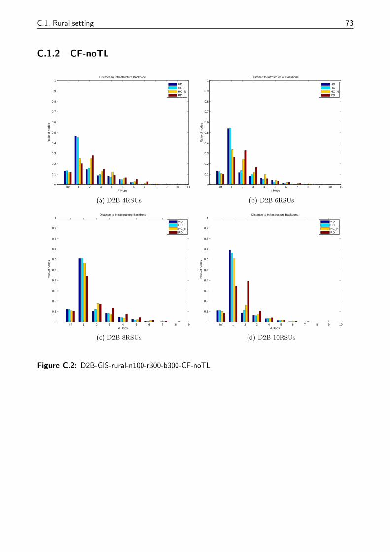
C.1. Rural setting 73
C.1.2 CF-noTL
Inf 1 2 3 4 5 6 7 8 9 10 110
0.1
0.2
0.3
0.4
0.5
0.6
0.7
0.8
0.9
1
# Hops
Rat
io o
f nod
es
Distance to Infrastructure Backbone
HDHCHC_NRD
(a) D2B 4RSUs
Inf 1 2 3 4 5 6 7 8 9 10 110
0.1
0.2
0.3
0.4
0.5
0.6
0.7
0.8
0.9
1
# Hops
Rat
io o
f nod
es
Distance to Infrastructure Backbone
HDHCHC_NRD
(b) D2B 6RSUs
Inf 1 2 3 4 5 6 7 8 90
0.1
0.2
0.3
0.4
0.5
0.6
0.7
0.8
0.9
1
# Hops
Rat
io o
f nod
es
Distance to Infrastructure Backbone
HDHCHC_NRD
(c) D2B 8RSUs
Inf 1 2 3 4 5 6 7 8 9 100
0.1
0.2
0.3
0.4
0.5
0.6
0.7
0.8
0.9
1
# Hops
Rat
io o
f nod
es
Distance to Infrastructure Backbone
HDHCHC_NRD
(d) D2B 10RSUs
Figure C.2: D2B-GIS-rural-n100-r300-b300-CF-noTL
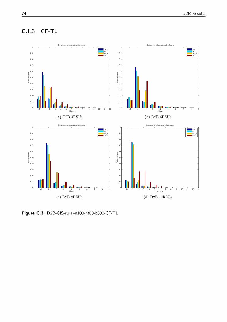
74 D2B Results
C.1.3 CF-TL
Inf 1 2 3 4 5 6 7 8 9 10 11 12 130
0.1
0.2
0.3
0.4
0.5
0.6
0.7
0.8
0.9
1
# Hops
Rat
io o
f nod
es
Distance to Infrastructure Backbone
HDHCHC_NRD
(a) D2B 4RSUs
Inf 1 2 3 4 5 6 7 8 90
0.1
0.2
0.3
0.4
0.5
0.6
0.7
0.8
0.9
1
# Hops
Rat
io o
f nod
es
Distance to Infrastructure Backbone
HDHCHC_NRD
(b) D2B 6RSUs
Inf 1 2 3 4 5 6 7 8 90
0.1
0.2
0.3
0.4
0.5
0.6
0.7
0.8
0.9
1
# Hops
Rat
io o
f nod
es
Distance to Infrastructure Backbone
HDHCHC_NRD
(c) D2B 8RSUs
Inf 1 2 3 4 5 6 7 8 9 10 11 12 130
0.1
0.2
0.3
0.4
0.5
0.6
0.7
0.8
0.9
1
# Hops
Rat
io o
f nod
es
Distance to Infrastructure Backbone
HDHCHC_NRD
(d) D2B 10RSUs
Figure C.3: D2B-GIS-rural-n100-r300-b300-CF-TL
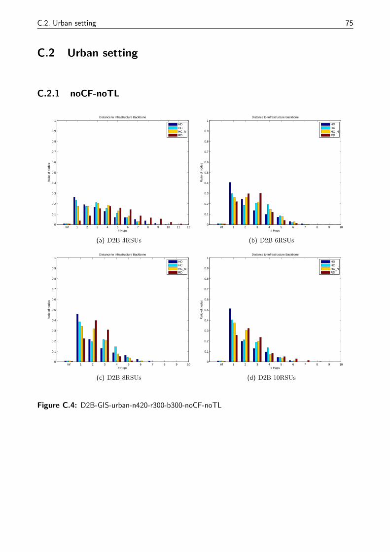
C.2. Urban setting 75
C.2 Urban setting
C.2.1 noCF-noTL
Inf 1 2 3 4 5 6 7 8 9 10 11 120
0.1
0.2
0.3
0.4
0.5
0.6
0.7
0.8
0.9
1
# Hops
Rat
io o
f nod
es
Distance to Infrastructure Backbone
HDHCHC_NRD
(a) D2B 4RSUs
Inf 1 2 3 4 5 6 7 8 9 100
0.1
0.2
0.3
0.4
0.5
0.6
0.7
0.8
0.9
1
# Hops
Rat
io o
f nod
es
Distance to Infrastructure Backbone
HDHCHC_NRD
(b) D2B 6RSUs
Inf 1 2 3 4 5 6 7 8 9 100
0.1
0.2
0.3
0.4
0.5
0.6
0.7
0.8
0.9
1
# Hops
Rat
io o
f nod
es
Distance to Infrastructure Backbone
HDHCHC_NRD
(c) D2B 8RSUs
Inf 1 2 3 4 5 6 7 8 9 100
0.1
0.2
0.3
0.4
0.5
0.6
0.7
0.8
0.9
1
# Hops
Rat
io o
f nod
es
Distance to Infrastructure Backbone
HDHCHC_NRD
(d) D2B 10RSUs
Figure C.4: D2B-GIS-urban-n420-r300-b300-noCF-noTL

76 D2B Results
C.2.2 CF-noTL
Inf 1 2 3 4 5 6 7 8 9 10 110
0.1
0.2
0.3
0.4
0.5
0.6
0.7
0.8
0.9
1
# Hops
Rat
io o
f nod
es
Distance to Infrastructure Backbone
HDHCHC_NRD
(a) D2B 4RSUs
Inf 1 2 3 4 5 6 7 8 9 10 11 12 130
0.1
0.2
0.3
0.4
0.5
0.6
0.7
0.8
0.9
1
# Hops
Rat
io o
f nod
es
Distance to Infrastructure Backbone
HDHCHC_NRD
(b) D2B 6RSUs
Inf 1 2 3 4 5 6 7 8 9 100
0.1
0.2
0.3
0.4
0.5
0.6
0.7
0.8
0.9
1
# Hops
Rat
io o
f nod
es
Distance to Infrastructure Backbone
HDHCHC_NRD
(c) D2B 8RSUs
Inf 1 2 3 4 5 6 7 8 9 100
0.1
0.2
0.3
0.4
0.5
0.6
0.7
0.8
0.9
1
# Hops
Rat
io o
f nod
es
Distance to Infrastructure Backbone
HDHCHC_NRD
(d) D2B 10RSUs
Figure C.5: D2B-GIS-urban-n420-r300-b300-CF-noTL

C.2. Urban setting 77
C.2.3 CF-TL

78 D2B Results
C.3 City setting
C.3.1 noCF-noTL

C.3. City setting 79
C.3.2 CF-noTL

80 D2B Results
C.3.3 CF-TL
Bibliography
[1] Cooperative Vehicle-Infrastructure Systems. URL http://www.cvisproject.org/.
[2] Dedicated Short Range Communications. URL http://www.leearmstrong.com/DSRC/
DSRCHomeset.htm.
[3] Generic Mobility Simulation Framework. URL http://polar9.ethz.ch/gmsf/.
[4] URL http://www.stanford.edu/~dgleich/programs/matlab_bgl/.
[5] URL http://sumo.sourceforge.net/index.shtml.
[6] SmartWay. URL http://www.epa.gov/smartway/.
[7] URL http://www.analytictech.com/ucinet/ucinet.htm.
[8] . URL http://www.vehicle-infrastructure.org/.
[9] . URL http://www.viicalifornia.org/.
[10] Realistic vehicular traces. URL http://lst.inf.ethz.ch/ad-hoc/car-traces/.
[11] R. Baldessari, A. Festag, A. Matos, J. Santos, and R. Aguiar. Flexible ConnectivityManagement in Vehicular Communication Networks. In Workshop on Intelligent Trans-portation (WIT 2006), pages 211–216, 2006.
[12] U. Brandes. On variants of shortest-path betweenness centrality and their generic compu-tation. Social Networks, 2008.
[13] G. Calandriello, P. Papadimitratos, A. Lioy, and J.-P. Hubaux. Efficient and RobustPseudonymous Authentication in VANET. In VANET 2007, Montreal, 2007. ACM.
[14] I. Carreras, D. Miorandi, G. Canright, and K. Engo-Monsen. Eigenvector Centrality inHighly Partitioned Mobile Networks: Principles and Applications. Springer, 2007.
[15] M. Cops. VII Strategy for Safety and Mobility, 2007.
[16] B. Cornwell. A Complement-Derived Centrality Index for Disconnected Graphs. INSNA,pages 70–81, 2005.
[17] P. Crucitti, V. Latora, and S. Porta. Centrality Measures in Spatial Networks of UrbanStreets. Physical Review E (Statistical, Nonlinear, and Soft Matter Physics), 73(3):036125,2006. doi: 10.1103/PhysRevE.73.036125.
82 BIBLIOGRAPHY
[18] E.M. Daly and M. Haahr. Social network analysis for routing in disconnected delay-tolerantmanets. In MobiHoc ’07: Proceedings of the 8th ACM international symposium on Mobilead hoc networking and computing, 2007.
[19] L. C. Freeman. Centrality in social networks: Conceptual clarification. Social Networks,1979.
[20] J. Freudiger, M. Raya, M. Felegyhazi, P. Papadimitratos, and J.-P. Hubaux. Mix-Zonesfor Location Privacy in Vehicular Networks. In ACM Workshop on Wireless Networkingfor Intelligent Transportation Systems (WiN-ITS), Vancouver, 2007.
[21] H. Habiba and T. Y. Berger-Wolf. Maximizing the extent of spread in dynamic network.Technical report, DIMACS, 2007.
[22] H. Habiba, C. Tantipathananandh, and T. Y. Berger-Wolf. Betweenness Centrality Mea-sure in Dynamic Networks. Technical report, DIMACS, 2007.
[23] I. W. H. Ho, K. K. Leung, J. W. Polak, and R. Mangharam. Node Connectivity inVehicular Ad Hoc Networks with Structured Mobility. In LCN ’07: Proceedings of the32nd IEEE Conference on Local Computer Networks, pages 635–642, Washington, DC,USA, 2007. IEEE Computer Society.
[24] M. Kafsi, O. Dousse, P. Papadimitratos, T. Alpcan, and J.-P. Hubaux. VANET Connec-tivity Analysis. Technical report, EPFL/T-Labs, 2008.
[25] V. Naumov, R. Baumann, and T. Gross. An Evaluation of Inter-Vehicle Ad Hoc NetworksBased on Realistic Vehicular Traces. In In Proceedings of The Seventh ACM InternationalSymposium on Mobile Ad Hoc Networking and Computing (MobiHoc’06), 2006.
[26] M.E.J. Newman. A measure of betweenness centrality based on random walks. SocialNetworks, 2005.
[27] P. Papadimitratos, V. Gligor, and J.-P. Hubaux. Securing Vehicular Communications -Assumptions, Requirements, and Principles. In Workshop on Embedded Security in Cars(ESCAR) 2006, 2006.
[28] S. Porta, P. Crucitti, and V. Latora. The Network Analysis of Urban Streets: A PrimalApproach. ArXiv Condensed Matter e-prints, 2005.
[29] M. Raya and J.-P. Hubaux. The Security of Vehicular Ad Hoc Networks. In SASN 2005,pages 11–21, 2005.
[30] M. Raya, A. Aziz, and J. P. Hubaux. Efficient Secure Aggregation in VANETs. In VANET2006, pages 67–75, 2006.
[31] B. Smith, B. Park, H. Tanikella, and G. Zhang. Preparing to use vehicle infrastructureintegration in transportation operations: phase i. Technical report, Virgina TransportationResearch Council, 2008.
[32] P. Sommer. Design and Analysis of Realistic Mobility Model for Wireless Mesh Networks.Master’s thesis, ETH Zurich, 2007.
[33] M. Treiber, A. Hennecke, and D. Helbing. Congested Traffic States in Empirical Observa-tions and Microscopic Simulations. Physical Review E, 62:1805, 2000.

BIBLIOGRAPHY 83
[34] S. Wasserman and K. Faust. Social Network Analysis: Methods and Applications. Cam-bridge University Press, 1994.
[35] X. Yang, J. Liue, F. Zhao, and N. H. Vaidya. A Vehicle-to-Vehicle Communication Proto-col for Cooperative Collision Warning. First Annual International Conference on Mobileand Ubiquitous Systems: Networking and Services (MobiQuitous’04), pages 114–123, 2004.